THE SPATIAL CLUSTERING OF STAR-FORMING GALAXIES AT REDSHIFTS $1.4\lower 2.15277pt\hbox{$\;\buildrel<\over{\sim}\;$}z\lower 2.15277pt\hbox{$\;\buildrel<\over{\sim}\;$}3.5$

Abstract

We analyzed the spatial distribution of $28500$ photometrically selected galaxies with magnitude $23.5<{\cal R}_{\rm AB}<25.5$ and redshift $1.4<z<3.5$ in 21 fields with a total area of $0.81$ square degrees. The galaxies were divided into three subsamples, with mean redshifts $\bar{z}=1.7$, $2.2$, $2.9$, according to the $U_{n}G{\cal R}$ selection criteria of Adelberger et al. (2004) and Steidel et al. (2003). Combining the galaxies’ measured angular clustering with redshift distributions inferred from $1600$ spectroscopic redshifts, we find comoving correlation lengths at the three redshifts of $r_{0}=4.5\pm 0.6$, $4.2\pm 0.5$, and $4.0\pm 0.6h^{-1}$ Mpc, respectively, and infer a roughly constant correlation function slope of $\gamma=1.6\pm 0.1$. We derive similar numbers from the $1600$ object spectroscopic sample itself with a new statistic, $K$, that is insensitive to many possible systematics. Galaxies that are bright in ${\cal R}$ ($\lambda_{\rm rest}\sim 1500$–$2500$Å) cluster more strongly than fainter galaxies at $z=2.9$ and $z=2.2$ but not, apparently, at $z=1.7$. Comparison to a numerical simulation that is consistent with recent WMAP observations suggests that galaxies in our samples are associated with dark matter halos of mass $10^{11.2}$–$10^{11.8}M_{\odot}$ ($z=2.9$), $10^{11.8}$–$10^{12.2}M_{\odot}$ ($z=2.2$), $10^{11.9}$–$10^{12.3}M_{\odot}$ ($z=1.7$), and that a small fraction of the halos contain more than one galaxy that satisfies our selection criteria. Adding recent observations of galaxy clustering at $z\sim 0$ and $z\sim 1$ to the simulation results, we conclude that the typical object in our samples will evolve into an elliptical galaxy by redshift $z=0$ and will already have an early-type spectrum by redshift $z=1$. We comment briefly on the implied relationship between galaxies in our survey and those selected with other techniques.

1. INTRODUCTION

Early investigators studied the spatial distribution of galaxies because they hoped to learn about the structure of the universe on the largest scales. Their influential work was superseded, in the end, by its competition. Problems began with the demonstration that galaxies contained only a small fraction of the matter in the universe. Galaxy formation remained too poorly understood to quell doubts about how faithfully galaxies traced underlying distribution of dark matter. Other observations improved—gravitational lensing, peculiar velocities, intergalactic absorption lines, and so on—and seemed easier to relate to matter fluctuations. Computers became fast enough to predict the evolution of the large-scale matter distribution from the the initial conditions that microwave-background missions were measuring with increasing precision. As it became clear that the simulations and observations agreed remarkably well, most researchers concluded that the large-scale structure of the universe could be understood completely as the product of gravitational instability amplifying small inflationary perturbations. Galaxies, once believed to be the primary constituent of the universe, came to be seen as small test particles swept into ever larger structures by converging dark matter flows.

The spatial distribution of galaxies remains interesting because it can teach us about galaxy formation. Galaxy formation must be closely related to larger process of gravitational structure formation, since the formation of a galaxy begins with gas streaming into a massive potential well and ends with stars drifting in the cosmic flow. Lessons from 20 years of numerical investigations into structure formation should therefore carry over to the analysis of galaxy clustering. One example is the known positive correlation between clustering strength and mass for virialized dark matter halos. Since galaxies reside in dark matter halos, their clustering strength provides an indication of the mass of the halos that contain them. The resulting mass estimate depends on the assumptions that the microwave background and other observations have given us reliable estimates of cosmological parameters and of the initial matter power-spectrum, that numerical simulations can correctly trace the evolution of the matter distribution, at least for moderate densities, and that no process can significantly separate baryons from dark matter on Mpc scales—assumptions that are at least as plausible as those behind competing techniques for mass estimation. Another example is the evolution in the clustering strength of a population of galaxies once it has formed. This is driven solely by gravity and is easy to predict from numerical simulations. Comparing the clustering of (say) galaxies in the local universe and those at high redshift can therefore suggest or rule out possible links between them. Few other methods are as useful for unifying into evolutionary sequences the galaxy populations we observe at different look-back times. An excellent review of the history of these techniques has been written by Giavalisco (2002; pp 620-624).

This paper has two aims. The first is to present measurements of the clustering of UV-selected star-forming galaxies in a redshift range $1.4<z<3.5$ that is only partially explored. Section 2 describes the way we obtained our data, § 3 describes and justifies the techniques we used to estimate the spatial clustering in our galaxy samples, and § 4 presents our estimates of the galaxy correlation function at redshifts $z\sim 1.7$, $z\sim 2.2$, and $z\sim 2.9$. The survey analyzed here is several times larger than its predecessors; the surveyed area of $0.81$ square degrees is roughly 700 times larger than the area analyzed by Arnouts et al. (2002) and 4 times larger than the areas analyzed by Giavalisco & Dickinson (2001) and Ouchi et al. (2001). The second aim is to discuss what our measurements imply about the galaxies and their descendants. In § 5.1 we show that the galaxies’ correlation functions are indistinguishable from those of virialized dark matter halos with mass $M\sim 10^{12}M_{\odot}$. In § 5.2 we show that the galaxies, dragged by gravity for billions of years, caught in the press of structure formation, would by redshift $z=0$ have a correlation function that is indistinguishable from that of the elliptical galaxies that surround us. Our results are summarized in § 6.

2. DATA

2.1. Observed

The data we analyzed were drawn from our ongoing surveys of high-redshift star-forming galaxies. A brief description of the surveys follows; see Steidel et al. (2003, 2004) for further details. Deep, multi-hour $U_{n}G{\cal R}$ images of 21 fields scattered around the sky were obtained with various 4m-class telescopes (table 1). Tens of thousands of objects were visible in these images. For the analysis of this paper we ignored all but the subset ($\sim$ 20%) with AB magnitude

$$23.5\leq{\cal R}\leq 25.5$$ (1)

and AB colors satisfying the “LBG” selection criteria of Steidel et al. (2003),

$$U_{n}-G \geq G-{\cal R}+1.0$$

$$G-{\cal R} \leq 1.2,$$ (2)

the “BX” selection criteria of Adelberger et al. (2004),

$$G-{\cal R} \geq -0.2$$

$$U_{n}-G \geq G-{\cal R}+0.2$$

$$G-{\cal R} \leq 0.2(U_{n}-G)+0.4$$

$$U_{n}-G < G-{\cal R}+1.0,$$ (3)

or the “BM” selection criteria of Adelberger et al. (2004),

$$G-{\cal R} \geq -0.2$$

$$U_{n}-G \geq G-{\cal R}-0.1$$

$$G-{\cal R} \leq 0.2(U_{n}-G)+0.4$$

$$U_{n}-G < G-{\cal R}+0.2.$$ (4)

In this range of ${\cal R}$ magnitudes, the colors are characteristic of galaxies at $1.4\lower 2.15277pt\hbox{$\;\buildrel<\over{\sim}\;$}z\lower 2.15277pt\hbox{$\;\buildrel<\over{\sim}\;$}3.3$. (The restriction to ${\cal R}>23.5$ helps eliminate most interlopers; see Adelberger et al. 2004 and Steidel et al. 2004.) By obtaining spectra of more than $1600$ galaxies with these colors, Steidel et al. (2003, 2004) established that the mean redshift and $\pm 1\sigma$ range of galaxies in the three samples is

$$\bar{z}\pm\sigma_{z}=\cases{2.94\pm 0.30&LBG\cr 2.24\pm 0.37&BX\cr 1.69\pm 0.36&BM.\cr}$$ (5)

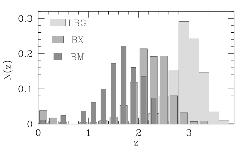
(These values exclude galaxies with ${\cal R}<23.5$ or ${\cal R}>25.5$ as well as the handful of low-redshift “interloper” galaxies with $z<0.8$.) Redshift histograms are shown in figure 1. We will use the term “photometric candidates” to describe the objects with $23.5\leq{\cal R}\leq 25.5$ whose colors satisfy one set of the selection criteria presented above, and the term “spectroscopic sample” to describe the subset of photometric candidates that had a spectroscopic redshift measured by Steidel et al. (2003) or Steidel et al. (2004). Although the spectroscopic sample is sizeable, it contains only a small fraction ($\lower 2.15277pt\hbox{$\;\buildrel<\over{\sim}\;$}10$%) of the photometric candidates (see figure 2 and table 1).

Table 1Observed fields

Name	$\Delta\Omega$	$N_{\rm LBG}$	$N_{\rm BX}$	$N_{\rm BM}$	${\cal I}_{\rm LBG}$	${\cal I}_{\rm BX}$	${\cal I}_{\rm BM}$
3c324	$6.6\times 6.6$	11/49	0/166	0/126	0.0035	0.0034	0.0042
B20902	$6.3\times 6.5$	31/65	1/207	0/189	0.0036	0.0035	0.0043
CDFa	$8.7\times 8.9$	34/99	0/336	0/280	0.0029	0.0028	0.0036
CDFb	$9.0\times 9.1$	20/120	0/316	0/273	0.0028	0.0028	0.0035
DSF2237a	$9.0\times 9.1$	39/100	1/367	0/328	0.0028	0.0028	0.0035
DSF2237b	$8.9\times 9.1$	44/161	1/516	0/309	0.0028	0.0028	0.0035
HDF	$10.4\times 14.4$	54/187	128/735	37/587	0.0022	0.0022	0.0028
Q0201	$8.6\times 8.7$	18/90	4/339	0/285	0.0029	0.0029	0.0036
Q0256	$8.5\times 8.4$	45/126	1/346	0/243	0.0030	0.0029	0.0037
Q0302	$15.6\times 15.7$	46/824	0/1778	0/749	0.0018	0.0018	0.0023
Q0933	$8.9\times 9.2$	63/192	0/435	0/273	0.0028	0.0028	0.0035
Q1307	$16.3\times 16.0$	16/483	47/1352	9/936	0.0017	0.0017	0.0023
Q1422	$7.3\times 15.6$	96/253	1/728	0/491	0.0024	0.0024	0.0030
Q1623	$12.0\times 22.3$	6/462	189/1220	2/847	0.0016	0.0016	0.0022
Q1700	$15.4\times 15.4$	15/406	62/1456	1/948	0.0018	0.0018	0.0024
Q2233	$9.2\times 9.2$	44/76	1/267	0/181	0.0028	0.0028	0.0035
Q2343	$22.8\times 11.5$	10/385	148/938	8/541	0.0016	0.0016	0.0022
Q2346	$16.5\times 17.1$	1/362	34/1142	1/754	0.0016	0.0017	0.0022
SSA22a	$8.6\times 8.9$	42/151	10/360	1/253	0.0029	0.0028	0.0036
SSA22b	$8.6\times 8.9$	29/73	5/281	1/308	0.0029	0.0028	0.0036
Westphal	$14.9\times 15.1$	172/270	43/724	20/632	0.0018	0.0018	0.0024
Total	2907	836/4934	676/14009	80/9533	0.0021	0.0021	0.0029

Figure 1.— Redshift distributions of objects whose colors satisfy the three sets of selection criteria presented in § 2.1.

Figure 2.— The number of objects in the spectroscopic and photometric samples as a function of ${\cal R}$ magnitude.

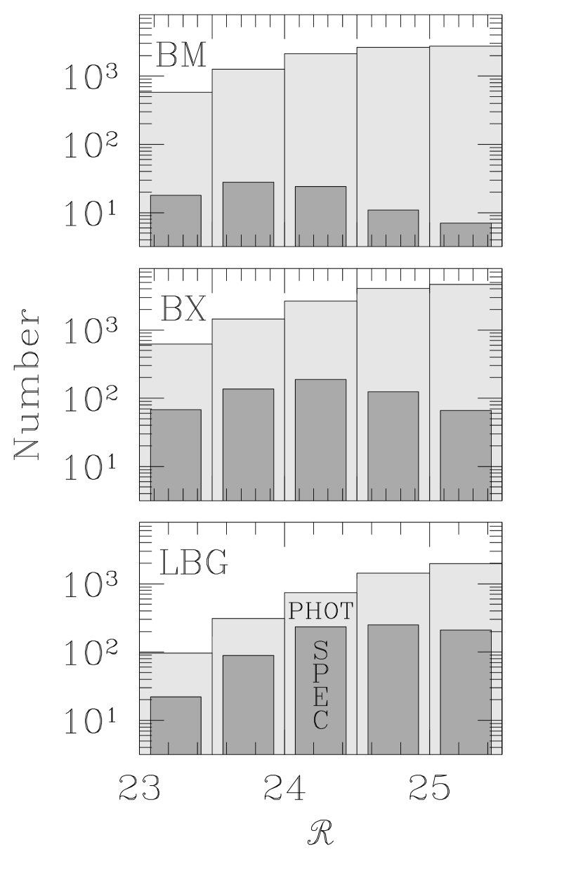
All redshifts were measured with the Low-Resolution Imaging Spectrograph (LRIS; Oke et al. 1995) on the Keck telescopes. The number of redshifts in each field was determined by the number of clear nights that were allocated. Photometric candidates were selected for spectroscopy more-or-less at random, but in one way the selection was far from random: spectroscopic objects in each field were constrained to fit together in a non-interfering way on one of a small number of multislit masks. This introduced artificial angular clustering to the spectroscopic samples, particularly in fields where our image’s size significantly exceeded the spectrograph’s $\sim 8^{\prime}$ field-of-view. In some cases the artificial angular clustering was increased by our desire to obtain particularly dense spectroscopic sampling in some parts of an image, e.g., near a background QSO.

Table 1 lists the number of BM, BX, and LBG photometric candidates and spectroscopic galaxies in each field. The field-to-field variations in the number of photometric candidates per square arcminute were caused primarily by differences in exposure times, seeing, sky brightness, telescope plus instrumental throughput, and so on, from one run to the next. Recall that we used many different telescopes and cameras during our imaging survey. The expected variations in intrinsic surface density (also shown in the table, and calculated for galaxies with bias $b=1$ as described in § 3.1 below) are significantly smaller.

We estimated the angular correlation functions from the lists of photometric candidates. Inferring a comoving correlation length $r_{0}$ from the measured angular clustering required an estimate of the objects’ redshift distribution. For this we took the measured redshift distributions of the spectroscopic samples. Since the spectroscopic samples are large—several hundred for the BX and LBG criteria, nearly 100 for BM—random fluctuations are unlikely to have given redshift distributions to them that are significantly different from those of the parent photometric samples. We were able to measure a redshift for only $\sim 80$% of the objects we observed spectroscopically, however, and it is therefore possible that various systematics (e.g., difficulties measuring spectroscopic redshifts for galaxies in certain redshift ranges) could have caused the spectroscopic and photometric samples to have somewhat different redshift distributions. Repeated observations of a subset of the initial spectroscopic failures show that these objects have the same redshift distribution as the initial successes, implying that any systematics are not severe.

2.2. Simulated

To help us interpret our observations, we refered at times the GIF-LCDM numerical simulation of structure formation in a cosmology with $\Omega_{M}=0.3$, $\Omega_{\Lambda}=0.7$, $h=0.7$, $\Gamma=0.21$, and $\sigma_{8}=0.9$. This gravity-only simulation contained $256^{3}$ particles with mass $1.4\times 10^{10}h^{-1}M_{\odot}$ in a periodic cube of comoving side-length $141.3h^{-1}$ Mpc, used a softening length of $20h^{-1}$ comoving kpc, and was released publicly, along with its halo catalogs, by Frenk et al. astro-ph/0007362. Further details can be found in Jenkins et al. (1998) and Kauffmann et al. (1999). Since the GIF-LCDM cosmology is consistent with the Wilkinson Microwave-Anisotropy Probe results (Spergel et al. 2003), and since modeling the gravitational growth of perturbations on large ($\sim$ Mpc) scales is not numerically challenging, we will assume that the growth of structure found in this simulation closely mirrors the growth of structure in the actual universe.

For our purposes the most interesting aspect of the simulation is the spatial distribution of virialized “halos”, or overdensities with $\delta\rho/\rho\sim 200$, since these deep potential wells are the sites where galaxies can form from cooling gas. The public halo catalogs were created, by the GIF team, by running a halo-finding algorithm at various time steps in the simulation. We will say that all the halos identified by the algorithm at time-step $t=156$ (say) had $t=156$ as their time of identification. Correlation functions for halos at the time of identification were calculated directly from the public halo catalogs. In subsequent time-steps these halos were progressively displaced by gravity. Some grew; others were destroyed as they were subsumed into larger structures. Any galaxies within the halos would be likely to survive intact, however, and it is interesting to trace the expected evolution in their correlation function over time. To do this, we assumed that the galaxies in a halo would be displaced by gravity by the same amount, and in the same direction, as the halo’s most bound particle. If $\{p_{i}\}$ denotes the set of particles that were the most bound particle in a halo at $t_{\rm earlier}$, we assumed that the correlation function at time $t_{\rm later}$ of the galaxies that lay within halos identified at time $t_{\rm earlier}$ would be roughly equal to the correlation function of particles $\{p_{i}\}$ at time $t_{\rm later}$. At spatial separations that are large compared to the typical halo radius, the expected evolution of the galaxy correlation function is insensitive to the details of this procedure. These are the only spatial separations we will consider. Our focus on large spatial scales also justifies our ignoring the possibility of galaxy mergers. Although mergers can strongly affect the correlation function on small scales, on large scales the effect is more subtle. It can be understood as follows. At time $t_{\rm later}$, the galaxies identified at time $t_{\rm earlier}$ will be found in halos with a range of masses, and their large-scale correlation function will be a weighted average of the correlation functions of the halos. Since the weighting depends on typical number of descendant galaxies in halos of each mass, and since halos with different masses have different correlation functions, the large-scale correlation function of descendant galaxies will be altered by mergers if the merger frequency depends on halo mass. In practice, however, the difference in correlation functions between the more massive and less massive halos that host the descendants is not enormous, and as a result the merger frequency would have to be an implausibly strong function of halo mass to alter the descendant correlation functions on large scales in a significant way.

3. METHODS

Two approaches will be used to estimate the clustering strength. The first approach, which is standard, relies almost exclusively on the angular positions of the galaxies. The second relies almost exclusively on the galaxies’ measured redshifts. These approaches exploit different aspects of our data and are subject to different systematics. The level of agreement between them provides an important test of our conclusions’ robustness. This section describes and justifies the two approaches. Readers interested primarily in our scientific results may wish to skip ahead to § 4.

3.1. Angular clustering

The observed clustering of galaxies on the plane of the sky is related to the galaxies’ three-dimensional correlation function in a straightforward way. Let $z$ denote a galaxy’s redshift and ${\bf\Theta}$ denote its angular position. ${\bf\Theta}$ is written in bold face because two numbers (e.g., right ascension and declination) are required to specify the galaxy’s angular position. If $P(z_{1}{\bf\Theta_{1}}|z_{2}{\bf\Theta_{2}})$ is the probability that a galaxy at known position $(z_{2},{\bf\Theta_{2}})$ has a neighbor at position $(z_{1},{\bf\Theta_{1}})$, then elementary identities show that the probability that a galaxy at angular position ${\bf\Theta_{2}}$ will have a neighbor at angular position ${\bf\Theta_{1}}$ is

$$P({\bf\Theta_{1}}|{\bf\Theta_{2}})=\int dz_{1}dz_{2}P(z_{2}|{\bf\Theta_{2}})P(z_{1}{\bf\Theta_{1}}|z_{2}{\bf\Theta_{2}}).$$ (6)

Observations indicate that the reduced correlation function is well approximated by an isotropic power law,

$$P(z_{1}{\bf\Theta_{1}}|z_{2}{\bf\Theta_{2}})\simeq P(z_{1}{\bf\Theta_{1}})\bigl{[}1+(r_{12}/r_{0})^{-\gamma}\bigr{]},$$ (7)

where $r_{0}$ and $\gamma$ parametrize the shape of the power law and $r_{12}$ is the distance between $(z_{1},{\bf\Theta_{1}})$ and $(z_{2},{\bf\Theta_{2}})$. This implies, in the circumstances of interest to us, that the reduced angular correlation function will also be a power law,

$$P({\bf\Theta_{1}}|{\bf\Theta_{2}})=P({\mathbf{\Theta}_{1}})(1+A\theta_{12}^{-\beta})$$ (8)

with $\beta\equiv\gamma-1$. If the angular separation $\theta_{12}\equiv|{\bf\Theta_{1}}-{\bf\Theta_{2}}|$ between the galaxies is small, $\theta_{12}\ll 1$, and if the comoving correlation length $r_{0}$ does not change significantly from the front to the back of the survey, then

$$A = r_{0}^{\gamma}B\biggl{(}\frac{1}{2},\frac{\gamma-1}{2}\biggr{)}\int_{0}^{\infty}dz\,N^{2}(z)f^{1-\gamma}g^{-1}$$ (9)

$$\quad\quad\quad\quad\quad\quad\quad\quad\quad\Bigg{/}\Biggl{[}\int_{0}^{\infty}dz^{\prime}\,N(z^{\prime})\Biggr{]}^{2}$$

(see, e.g., Totsuji & Kihara 1969) where $N(z)$ is the survey selection function, $B$ is the beta function in the convention of Press et al. (1992), $g(z)\equiv c/H(z)$ is the change in comoving distance with redshift, $f(z)\equiv(1+z)D_{A}(z)$ is the change in comoving distance with angle, and $D_{A}(z)$ is the angular diameter distance. This follows from the relationship $\int_{-\infty}^{\infty}dz\,[r_{0}^{2}/(R^{2}+z^{2})]^{\gamma/2}=r_{0}^{\gamma}R^{1-\gamma}B(1/2,(\gamma-1)/2)$.

Our first approach to estimating the three dimensional clustering strength will be to measure the parameters $A$ and $\beta$ of the reduced angular correlation function $\omega(\theta)\equiv A\theta^{-\beta}$, then infer values for $r_{0}$ and $\gamma$ using the relationships above. Our estimates of $\omega(\theta)$ in different angular bins will be based on the Landy-Szalay (1993) estimator

$$\omega_{LS}(\theta)\equiv\frac{DD(\theta)-2DR(\theta)+RR(\theta)}{RR(\theta)}$$ (10)

where $DD(\theta)$ is the observed number of unique galaxy pairs with separation $\theta-\Delta\theta/2<\theta<\theta+\Delta\theta/2$, $DR(\theta)$ is the number of unique pairs with separation in the same range between the observed galaxy catalog and a galaxy catalog with random angular positions, and $RR(\theta)$ is the number of unique pairs in the random catalog with separations in the same range. In practice we reduce the noise in the random pair counts by creating random catalogs with many times more objects than the data catalogs ($n_{\rm rand}/n_{\rm data}\sim 100$), calculating $DR$ and $RR$, then multiplying $DR$ and $RR$ by $(n_{\rm data}-1)/n_{\rm rand}$ and $n_{\rm data}(n_{\rm data}-1)/[n_{\rm rand}(n_{\rm rand}-1)]$, respectively.

3.1.1 Integral constraint

Unless fluctuations on the size of our typical field-of-view are negligible, the number of detected galaxies in any field will be somewhat higher or lower than in a fair sample of the universe, and the number of galaxies in the field’s ideal random catalog would therefore be lower or higher than the observed number. As a result the values $DR$ and $RR$ that we calculate with our approach will be incorrect to some degree. In a single field this can make the clustering appear stronger or weaker than it truly is, but when many fields are averaged it tends to make the observed clustering appear artificially weak. This can be shown as follows. Assume that the observed mean density in a field differs from the global average by the unknown factor $1+\delta$, i.e., $\rho_{\rm obs}=\bar{\rho}(1+\delta)$, and let $DR$ and $RR$ be the pair counts calculated from scaling the random catalogs to the observed density. One might guess that the estimator of equation 10 ought to have $DR$ and $RR$ replaced by values corrected to the true mean density, i.e., by $DR/(1+\delta)$ and $RR/(1+\delta)^{2}$, and indeed Hamilton (1993, §3) has shown that the estimator

$$\omega_{\rm ideal}\equiv\frac{DD-2DR/(1+\delta)+RR/(1+\delta)^{2}}{RR/(1+\delta)^{2}}$$ (11)

is equal to the true angular correlation function on average,

$$\langle\omega_{\rm ideal}(\theta)\rangle=\omega(\theta).$$ (12)

This equation does not help us directly, since we do not know $\delta$ and cannot calculate $\omega_{\rm ideal}$, but it does show that the estimator $\omega_{LS}(\theta)$ must be biased:

$$\langle\omega_{LS}(\theta)\rangle=\omega(\theta)-\sigma^{2}\frac{DD}{RR}\simeq\omega(\theta)-\sigma^{2}$$ (13)

where $\sigma^{2}\equiv{\rm Var}(\delta)$ and the approximation assumes the weak clustering ($\omega\ll 1$) limit. It is therefore customary to estimate $\omega(\theta)$ by adding a constant ${\cal I}\equiv\omega(\theta)-\omega_{LS}(\theta)$ to the calculated values $\omega_{LS}$. The constant ${\cal I}$ depends on the unknown values of $\delta$ in the observed field or fields and cannot be calculated exactly. If $\sigma^{2}\ll 1$, so that field-to-field fluctuations are in the linear regime and have a nearly Gaussian distribution, and if our data are drawn from $n$ independent fields with measured pair counts $DD_{i}$, $DR_{i}$, and $RR_{i}$, then the value of ${\cal I}$ appropriate to a given angular bin in our data set will have a variance of

$${\rm Var}({\cal I}) = \frac{1}{RR_{\rm tot}^{2}}\sum_{i=1}^{n}\Bigl{[}(4\sigma_{i}^{2}+2\sigma_{i}^{4})DD_{i}^{2}-8\sigma_{i}^{2}DD_{i}DR_{i}$$ (14)

$$\quad\quad\quad\quad\quad\quad\quad\quad\quad\quad+4\sigma^{2}DR_{i}^{2}\Bigr{]}$$

$$\simeq \frac{1}{RR_{\rm tot}^{2}}\sum_{i=1}^{n}2\sigma_{i}^{4}DD_{i}^{2}$$ (15)

around its expectation value

$$\langle{\cal I}\rangle = \frac{1}{RR_{\rm tot}}\sum_{i=1}^{n}\sigma_{i}^{2}DD_{i}.$$ (16)

Here $RR_{\rm tot}\equiv\sum_{i=1}^{n}RR_{i}$ is the sum over all fields of the random pair counts in the chosen angular bin. In practice $\langle{\cal I}\rangle$ and ${\rm Var}({\cal I})$ depend very weakly on which bin is chosen. Below we will take $\langle{\cal I}\rangle$ at $100^{\prime\prime}$ as our best guess at the correction ${\cal I}$. When it matters we will discuss the effect of the uncertainty in ${\cal I}$.

We use two approaches to estimate the size of the uncertainty $\sigma_{i}$ in the mean galaxy density of the $i$th field. Since

$$\sigma^{2}\equiv\frac{1}{\Omega^{2}}\int_{\Omega}d\Omega_{1}\,d\Omega_{2}\,\omega(\theta_{12}),$$ (17)

it can be estimated numerically as

$$\sigma^{2}\simeq\sigma^{2}_{\rm num}\equiv\frac{\sum_{i}RR\,\omega(\theta_{i})}{\sum_{i}RR}$$ (18)

if $\omega(\theta_{i})$ is known (Infante 1994; Roche & Eales 1999). Unfortunately the iterative approach suggested by equations 13 and 18 can be unstable, at least when the correlation function slope is allowed to vary: a large value of $\omega_{LS}$ will imply a large correction $\sigma^{2}$, which implies an even larger $\omega_{LS}$ and even larger correction, and so on. The instability is undoubtedly worse for large images, where the estimate of the integral constraint correction for one iteration is completely dominated by the assumed correction from the previous. We were unable to use equation 18 as anything other than a consistency check.

A more robust estimate of $\sigma^{2}$ follows from theoretical considerations. Since matter fluctuations will still be in the linear regime on the large scales of our observations, the relative variance of mass from one surveyed volume to the next can be estimated from the linear cold-dark matter power-spectrum $P_{L}(k)$ (Bardeen et al. 1986; we adopt the parameters $\Gamma=0.2$, $\sigma_{8}=0.9$, $n=1$) with Parseval’s relationship

$$\sigma^{2}_{\rm CDM}=\frac{1}{(2\pi)^{3}}\int d^{3}kP_{L}(|{\mathbf{k}}|)|W_{k}^{2}({\mathbf{k}})|$$ (19)

where $W_{k}$ is the Fourier transform of a survey volume. The shape of the observed volume in any one of our fields is reasonably approximated in the radial direction by a Gaussian with comoving width (rms) $l_{z}$ and in the transverse directions by a rectangle with comoving dimensions $l_{x}\times l_{y}$. In this case

$$W_{k}=\exp\Bigl{[}-\frac{k_{z}^{2}l_{z}^{2}}{2}\Bigr{]}\frac{\sin(k_{x}l_{x}/2)}{k_{x}l_{x}/2}\frac{\sin(k_{y}l_{y}/2)}{k_{y}l_{y}/2}.$$ (20)

The implied value of $\sigma^{2}_{\rm CDM}$ for each sample in each field is shown in table 1; the values assume the powerspectrum normalization required for the r.m.s. fluctuation as a function of redshift in spheres of comoving radius $8h^{-1}$ Mpc to obey $\sigma_{8}(z)=\sigma_{8}(0)D_{L}(z)$ where $\sigma_{8}(0)=0.9$ and $D_{L}(z)$ is the linear growth factor to redshift $z$. The desired corrections $\sigma^{2}$ are then given by

$$\sigma^{2}\simeq b^{2}\sigma^{2}_{\rm CDM}$$ (21)

where $b$, the galaxy bias, is calculated from the ratio of galaxy to matter fluctuations in spheres of comoving radius $8h^{-1}$ Mpc:

$$b=\frac{\sigma_{8,{\rm g}}}{\sigma_{8}(z)}.$$ (22)

Here the galaxy variance

$$\sigma^{2}_{8,{\rm g}}=\frac{72(r_{0}/8h^{-1}\,\,{\rm Mpc})^{\gamma}}{(3-\gamma)(4-\gamma)(6-\gamma)2^{\gamma}}$$ (23)

(Peebles 1980 eq. 59.3) can be derived from the fit to the galaxy correlation function. This approach also requires an iterative solution, since the correction $\sigma^{2}$ to $\omega(\theta)$ depends on $\omega(\theta)$, but the advantage is that the assumed size of large-scale fluctuations is anchored in reality by our requirement that the slope of the correlation function match other observations on very large scales.

3.1.2 Uncertainties in the selection functions

The discussion so far assumes that we will know the precise shape of the selection function $N(z)$. In fact this is not true, and uncertainty in the true shape of our selection function is a source of error in the derived values of $r_{0}$. A larger width for the selection function means that projection effects are stronger, and therefore implies a larger value of $r_{0}$ for given angular clustering (see equation 9). If the selection function is a Gaussian with mean $\mu$ and standard deviation $\sigma_{\rm sel}$, and if the weak redshift variations of $f$ and $g$ can be ignored, then the constant $A$ in equation 9 is proportional to $\sigma_{\rm sel}^{-1}$, and the implied value of $r_{0}$ is proportional to $\sigma_{\rm sel}^{1/\gamma}$. Measuring $n$ redshifts drawn from this selection function determines $\mu$ to a precision $\sigma_{\rm sel}/n^{1/2}$ and $\sigma_{\rm sel}^{2}$ to a relative precision $2^{1/2}/(n-1)^{1/2}$. Excluding interlopers with $z<1$, we have measured roughly 800, 700, and 80 redshifts for galaxies in the LBG, BX, and BM samples, and the selection function width is $\sigma_{\rm sel}\sim 0.3$ for each. The relative uncertainty in $\sigma_{\rm sel}$ is therefore approximately $\sim 3$% for the LBG and BX samples and $\sim 9$% for the BM sample, which implies $\sim 2$% uncertainty in $r_{0}$ for the LBG and BX samples and $\sim 5$% uncertainty in the BM sample.

Variations of the selection function from one field to the next (owing, for example, to differences in the depth of the data or to systematic errors in our photometric zero points) are another source of concern, especially at the redshifts $z\sim 2$ where galaxies’ colors are insensitive to redshift and small color errors mimic large redshift differences. Suppose for simplicity that all fields have the same number of photometric candidates, let the rms width of the selection function in the $i$th field be written $\sigma_{i}=(1+\epsilon_{i})s$, where $s$ is the mean width among all fields, and let the mean redshift of the selection function be written $\mu+s\delta_{i}$ where $\mu$ is the mean redshift among all fields. Then the rms width of the total selection function

$$[{\rm Var}(z)]^{1/2}=s[1+{\rm Var}(\delta)+{\rm Var}(\epsilon)]^{1/2},$$ (24)

exceeds the value $s$ that should be used in determining $A$. Since we will (by necessity) use the total selection function in estimating $r_{0}$, our estimates will be biased high. Systematic errors in our zero points are unlikely to be larger than $\Delta m=0.05$, and variations in photometric depth will at most change our characteristic color uncertainties from $\sim 0.1$ to $\sim 0.2$ magnitudes. The measured variations in galaxy redshift with $U_{n}G{\cal R}$ color (see, e.g., Adelberger et al. 2004) imply (a) that zero point errors with $\Delta m=0.05$ will shift the mean redshifts of galaxies that satisfy the LBG, BX, and BM selection criteria by $\Delta z\simeq 0.01$, $0.13$, and $0.11$, respectively, and (b) that increasing the photometric uncertainty from $\sigma_{m}=0.1$ to $\sigma_{m}=0.2$ will increase the widths of the LBG, BX, and BM selection functions by $\sim 10$, $20$, and $20$%. The upper limits on ${\rm Var}(\delta)$ and ${\rm Var}(\epsilon)$ are therefore $0.002$ ($0.2$) and $0.01$ ($0.04$), respectively, for the LBG (BX,BM) sample. The required reduction in $r_{0}$ is negligible for the LBG sample but could be as large as $\sim 7$% for the other two. We will account for uncertainties in the selection function by decreasing the best-guess value of $r_{0}$ for the BM and BX samples by 3.5% and increasing the uncertainty in quadrature by $0.035r_{0}$.

3.1.3 Contaminants

As figure 1 shows, some fraction of the objects in the BX and BM samples will be low redshift interlopers. We correct for the resulting dilution in the clustering strength by using the full selection function, starting at $z=0$, in our estimate of $r_{0}$ from equation 9. This is the optimal correction only if the interlopers have the same comoving correlation length $r_{0}\sim 4h^{-1}$ Mpc (see below) as the galaxies in the primary samples. This should be nearly true, since Budavári et al. (2003) estimate $r_{0}=4.51\pm 0.19h^{-1}$ Mpc for the blue star-forming galaxy population at $z\sim 0.2$ from which our interlopers are drawn. In any case, since the correction itself is small—eliminating the tail with $z<1$ from $N(z)$ alters the inferred values of $r_{0}$ for the BM and BX samples by only $\sim 10$%—errors in it should not have an appreciable effect on our estimates of $r_{0}$.

3.2. Redshift clustering

We face three significant obstacles in trying to estimate the clustering strength from the spectroscopic catalogs.

(1) The objects in a given field that were selected for spectroscopy were not distributed randomly across the field, but were instead constrained to lie on one of a small number of multislit masks. Since only a small fraction of the galaxies were observed spectroscopically in the typical field, the finite size of the masks coupled with the need to avoid spectroscopic conflicts produced significant artificial clustering in the angular positions of sources in the spectroscopic catalog. The effect was worsened in some fields by our decision to obtain particularly dense spectroscopy near background QSOs. (2) Because galaxies’ $U_{n}G{\cal R}$ colors change slowly with redshift near $z\sim 2$, the expected redshift distribution $N(z)$ of our BM and BX color-selected samples depends sensitively on the quality of the photometry. The larger color errors from noisy photometry will lead to a broader $N(z)$, while relatively small systematic shifts in the photometric zero points can significantly alter the mean of $N(z)$. Adelberger et al. (2004) and § 3.1.2 of this paper discuss this point in more detail, but the upshot is that we cannot estimate the selection function $N(z)$ with great precision for the BX and BM samples. (3) Peculiar velocities and redshift uncertainties render imprecise our estimate of each galaxy’s position in the $z$ direction. This limits the accuracy of our estimate of the distance from one galaxy to its neighbors, complicating our efforts to measure the correlation function on small spatial scales.

Effects (1)–(3) are usually compensated with the aid of detailed simulations. Although this approach should work in principle, in practice it is hard for outsiders to evaluate whether the simulations were flawed. The remainder of this section describes the alternate approach that we adopt. It is based on analyzing observable quantities that are not affected by systematics (1)–(3).

The spurious angular clustering signal can be eliminated if we take the angular positions of spectroscopic galaxies as given and estimate the clustering strength solely from their redshifts. Let $Z$ be the comoving distance to redshift $z$, and let ${\mathbf{R}}\equiv(1+z)D_{A}(z){\bf\Theta}$ be the transverse comoving separation implied by the angular separation ${\bf\Theta}$ between a galaxy and some reference position, e.g., the center of the observed field. According to elementary probability identities, if we know that one galaxy has position $({\mathbf{R}_{2}},z_{2})$, then the probability that a second galaxy at transverse position ${\mathbf{R}_{1}}$ has radial position $Z_{1}$ is

$$P(Z_{1}|{\mathbf{R}_{1}}{\mathbf{R}_{2}}Z_{2})=\frac{P(Z_{1}{\mathbf{R}_{1}}|Z_{2}{\mathbf{R}_{2}})}{\int_{0}^{\infty}dZ_{1}^{\prime}P(Z_{1}^{\prime}{\mathbf{R}_{1}}|Z_{2}{\mathbf{R}_{2}})}$$ (25)

and the expected distribution of radial separations $Z_{12}\equiv Z_{1}-Z_{2}$ for galaxies with transverse separation $R_{12}\equiv|{\mathbf{R}_{1}}-{\mathbf{R}_{2}}|$ is

$$P(Z_{12}|R_{12}) = \int_{0}^{\infty}dZ_{2}\,P(Z_{2}|R_{12})P(Z_{12}|Z_{2}R_{12})$$ (27)

$$\simeq \bigl{[}1+\xi(R_{12},Z_{12})\bigr{]}\times$$

$$\quad\int_{0}^{\infty}dZ_{2}\,\frac{P(Z_{2})P(Z_{2}+Z_{12})}{1+P(Z_{2})r_{0}^{\gamma}R_{12}^{1-\gamma}\beta(\gamma)}$$

where we have used results from the previous section and adopted the shorthand $\beta(\gamma)$ for the beta-function given above, $\beta(\gamma)\equiv B(1/2,(\gamma-1)/2)$. (Equations 25 through 27 assume that the quantity $(1+z)D_{A}(z)$ is constant with redshift, an approximation that is valid for the small separations $|Z_{12}|\lower 2.15277pt\hbox{$\;\buildrel<\over{\sim}\;$}40h^{-1}$ comoving Mpc between the galaxy pairs we will use in this analysis.)

Equation 27 shows that the observable quantity $P(Z_{12}|R_{12})$ is sensitive to the clustering strength but independent of angular variations in the spectroscopic sampling density. Unfortunately the correlation function $\xi$ can be estimated from $P(Z_{12}|R_{12})$ with equation 27 only if we have a reasonably accurate estimate of the selection function shape $P(Z)$. This can be seen more clearly by Taylor-expanding the integral in equation 27 around $Z_{12}=0$ and approximating the selection function as a Gaussian with standard deviation $\sigma_{\rm sel}$ that is centered many standard deviations from $z=0$. One finds

$$P(Z_{12}|R_{12}) \simeq \Bigl{[}1+\xi(R_{12},Z_{12})\Bigr{]}\times$$ (28)

$$\quad\quad\Bigl{[}\frac{A_{0}}{\sigma_{\rm sel}}+\frac{A_{2}}{2\sigma_{\rm sel}^{3}}Z_{12}^{2}+\frac{A_{4}}{24\sigma_{\rm sel}^{5}}Z_{12}^{4}\Bigr{]}$$

where

$$A_{n}\equiv\int_{-\infty}^{\infty}du\,e^{-u^{2}}f_{n}(u)/g(u,R_{12}),$$

$f_{0}=1$, $f_{2}=u^{2}-1$, $f_{4}=u^{4}-6u^{2}+3$, $g\equiv 2\pi+(2\pi)^{1/2}a(R_{12})e^{-u^{2}/2}/\sigma_{\rm sel}$ and $a\equiv r_{0}^{\gamma}R_{12}^{1-\gamma}\beta(\gamma)$. The coefficients $A_{n}$ all have similar sizes since the integrals are dominated by contributions from $|u|\lower 2.15277pt\hbox{$\;\buildrel<\over{\sim}\;$}1$ where the integrands are of the same order.

In the angular clustering case above, inaccuracies in the adopted width $\sigma_{\rm sel}$ of the selection function affected the inferred amplitude of the correlation function but not its shape. Here they affect both. Moreover errors in $\sigma_{\rm sel}$ are multiplied not by $\xi$, but by $1+\xi$, which implies that they can easily dominate the true clustering signal when $\xi\ll 1$. Equation 28 shows that one must be careful estimating the strength of redshift clustering when the shape of the selection function is poorly known.

Our solution exploits the fact that $r_{0}\ll\sigma_{\rm sel}$ for our survey, which implies $Z_{12}\ll\sigma_{\rm sel}$ for all separations where $\xi$ is large enough to measure. As long as $Z_{12}\ll\sigma_{\rm sel}$, the terms proportional to $Z_{12}^{2}$ and $Z_{12}^{4}$ can be neglected in equation 28, and $P(Z_{12}|R_{12})$ will be very nearly equal to $C(R_{12})[1+\xi(R_{12},Z_{12})]$, with $C$ a function that does not depend on $Z_{12}$. The function $C$ does depend on the unknown selection function, but it can be eliminated by taking ratios of pair counts in a manner we discuss below. Ratios of $P(Z_{12}|R_{12})$ at fixed $R_{12}$ and different $Z_{12}$ will therefore be the basis of our estimate of the clustering strength in the spectroscopic sample; they are nearly immune to systematics from the irregular spectroscopic sampling and from the unknown selection function shape.

The final complication is the significant uncertainty $\sigma_{Z}$ in each object’s radial position $Z$ from peculiar velocities and redshift uncertainties. This uncertainty can be treated in various ways. We will follow the standard approach and estimate the value of the correlation function only within bins whose radial size $\Delta Z$ is large compared to $\sigma_{Z}$.

We are now ready to present the estimator that we adopt. Letting $N(a_{1},a_{2},R)$ denote the observed number of galaxy pairs with transverse separation $R$ and redshift separation $a_{1}\leq|Z_{12}|<a_{2}$, the discussion of the preceding paragraphs shows that the expected total number of pairs with radial separation $a_{1}\leq|Z_{12}|<a_{2}$ (and any transverse separation) is

$$\langle N_{\rm tot}(a_{1},a_{2})\rangle=2(a_{2}-a_{1})\sum_{i>j}^{\rm pairs}C(R_{ij})[1+\bar{\xi}_{a_{1},a_{2}}(R_{ij})]$$ (29)

where

$$\bar{\xi}_{a_{1},a_{2}}(R_{ij})\equiv\frac{1}{a_{2}-a_{1}}\int_{a_{1}}^{a_{2}}dZ\,\xi(R_{ij},Z).$$ (30)

As long as $N_{\rm tot}$ is large enough that

$$\Biggl{\langle}\frac{N_{\rm tot}(b_{1},b_{2})}{N_{\rm tot}(a_{1},a_{2})+N_{\rm tot}(b_{1},b_{2})}\Biggr{\rangle}\simeq\frac{\langle N_{\rm tot}(b_{1},b_{2})\rangle}{\langle N_{\rm tot}(a_{1},a_{2})+N_{\rm tot}(b_{1},b_{2})\rangle},$$ (31)

the ratio of pair counts

$$K_{a_{1},a_{2}}^{b_{1},b_{2}}\equiv\frac{N_{\rm tot}(b_{1},b_{2})}{N_{\rm tot}(a_{1},a_{2})+N_{\rm tot}(b_{1},b_{2})}$$ (32)

will have expectation value

$$\langle K_{a_{1},a_{2}}^{b_{1},b_{2}}\rangle \simeq \frac{N_{\rm exp}(b_{1},b_{2})}{N_{\rm exp}(a_{1},a_{2})+N_{\rm exp}(b_{1},b_{2})}$$ (33)

$$\simeq \frac{N^{\prime}_{\rm exp}(b_{1},b_{2})}{N^{\prime}_{\rm exp}(a_{1},a_{2})+N^{\prime}_{\rm exp}(b_{1},b_{2})}$$ (34)

regardless of angular selection effects, of uncertainties in the selection function, of peculiar velocities, and of redshift measurement errors, provided $a_{2}\ll\sigma_{\rm sel}$, $b_{2}\ll\sigma_{\rm sel}$, $a_{2}-a_{1}\gg\sigma_{Z}$, $b_{2}-b_{1}\gg\sigma_{Z}$, the selection function does not have strong features on scales smaller than $\sigma_{\rm sel}$, and $(1+z)D_{A}(z)$ varies slowly with $z$. Here $N_{\rm exp}(a_{1},a_{2})\equiv\langle N_{\rm tot}(a_{1},a_{2})\rangle$ is given by equation 29 and

$$N^{\prime}_{\rm exp}(a_{1},a_{2})=2(a_{2}-a_{1})\sum_{i>j}^{\rm pairs}[1+\bar{\xi}_{a_{1},a_{2}}(R_{ij})].$$

The second approximate equality in equation 34 exploits the fact that $C(R_{ij})$ is a very weak function of $R_{ij}$ in realistic situations. We estimate the correlation function from the spectroscopic sample by finding the parameters required to match the observed ratio $K_{a_{1},a_{2}}^{b_{1},b_{2}}$. In principle $K_{a_{1},a_{2}}^{b_{1},b_{2}}$ could be calculated separately for pairs in different bins of transverse separation $R_{ij}$, producing an estimate of the function $K_{a_{1},a_{2}}^{b_{1},b_{2}}(R)$ and allowing one to estimate both $r_{0}$ and $\gamma$ from the data. In practice a much larger sample is needed to fit for both $r_{0}$ and $\gamma$, so we hold $\gamma$ fixed and estimate $r_{0}$ only. Fortunately, as we will see, the best fit value of $r_{0}$ hardly changes as $\gamma$ is varied across the range allowed by the galaxies’ angular clustering.

The dependence of this estimator on the clustering strength is easy to understand intuitively. If the galaxies were unclustered ($\xi(r)=0$), we would observe the same number of pairs at every separation and $K_{a_{1},a_{2}}^{b_{1},b_{2}}$ would be equal, on average, to the ratio of the bin sizes $\eta\equiv(b_{2}-b_{1})/(b_{2}-b_{1}+a_{2}-a_{1})$. Correlation functions that peak near $r=0$ will produce more pairs in bins at smaller separations, driving $K_{a_{1},a_{2}}^{b_{1},b_{2}}$ away from $\eta$. The difference between $K_{a_{1},a_{2}}^{b_{1},b_{2}}$ and $\eta$ is sensitive to the strength of the clustering, and therefore can be used to estimate it. Adelberger (2005) uses Monte Carlo simulations to analyze the behavior of $K_{a_{1},a_{2}}^{b_{1},b_{2}}$ in more detail.

4. RESULTS

4.1. Angular

Figure 3 shows the raw (integral-constraint correction ${\cal I}=0$) values of the Landy-Szalay estimator $\omega_{LS}$ (equation 10) as a function of angular separation for galaxies in the three samples. We limited these data, and our subsequent fits, to angular separations $\theta<200^{\prime\prime}$, since at larger scales the weak angular-clustering signal could be swamped by various low-level systematics. The uncertainty $\sigma_{i}$ in each bin was taken to be the larger of $(DD_{i})^{1/2}/(RR_{i})$ (Peebles 1980, §48) and the observed standard deviation of the mean of $\omega_{LS}(\theta_{i})$ among the different fields in the survey. Typically the two were comparable. Numerical $\chi^{2}$ minimization produced the power-law fits shown with dashed lines. The correlation function parameters implied by the LBG fit, $r_{0}=3.35\pm 0.20h^{-1}$ comoving Mpc, $\gamma=1.74\pm 0.1$, agree well with the estimates of Giavalisco & Dickinson (2001) which also assumed ${\cal I}=0$. It is clear, however, that these parameters cannot be correct. Substituting them into equations 23, 22, and 21 shows that a significant correction ${\cal I}$ should have been applied to account for fluctuations on scales larger than the field-of-view. (Porciani & Giavalisco 2002 reached a similar conclusion, and derived a result for LBGs that agrees well with the integral-constraint-corrected result we present below.)

Figure 3.— Angular correlation functions uncorrected for the integral constraint ${\cal I}$. Points with error bars show the measured values of the estimator $\omega_{LS}$ for each sample. The dashed line shows the power-law $\omega=A\theta^{-\beta}$ that fits the data best. The solid histogram indicates the number of galaxy pairs ($/1000$) in each angular bin.

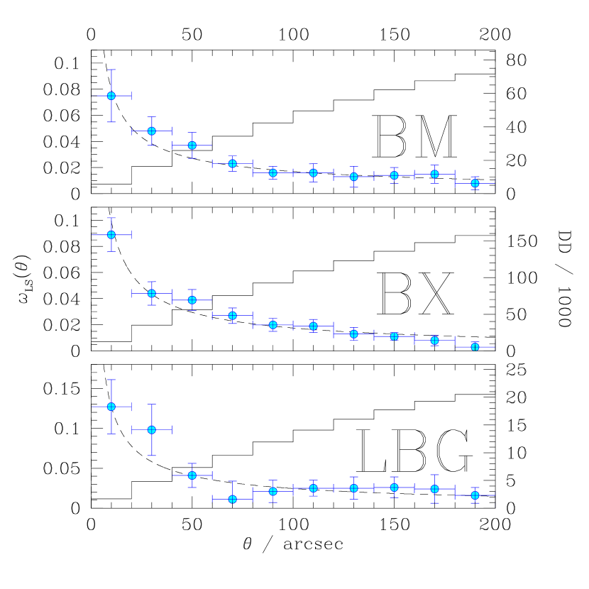
Figure 4 shows how our best-fit estimates of $r_{0}$ and $\gamma$ change as the correction ${\cal I}$ is applied. In our first iteration, described above, we assumed ${\cal I}=0$ and calculated the correlation function $\omega_{1}(\theta)$. For the second iteration we assumed the value of ${\cal I}$ implied by $\omega_{1}$ (equations 16, 23, 22, and 21) and estimated $\omega_{2}(\theta)$. For the third iteration we calculated ${\cal I}$ from $\omega_{2}(\theta)$. The process continued in this way until convergence. It settled on the same final parameters if we initially assumed a value for ${\cal I}$ that was too large. As figure 4 shows, the applied integral constraint corrections were comparable for each of the three samples. This is because the increase in ${\cal I}$ implied by the longer correlation lengths at lower redshifts happened to be cancelled by a decrease in ${\cal I}$ that resulted from the lower-redshift samples’ greater comoving depths.

Figure 4.— Effect of the integral constraint correction ${\cal I}$ on the inferred correlation function. The correction depends on the clustering strength and is therefore unknown initially. The figure illustrates the iterative approach described in the text. Small circles show the adopted value of ${\cal I}$ and the implied value of $r_{0}$ at each stage in the iteration. The numbers above points indicate the value of $\gamma$ for that iteration; for clarity they are given for only some iterations. Adopting the initial guess ${\cal I}=0$ leads to values of $r_{0},\gamma$ shown at ${\cal I}=0$ on the plot. Recalculating ${\cal I}$ for these values of $r_{0}$,$\gamma$ leads to the revised estimate of the correlation function parameters shown by the point just above and to the right. Follow the arrow. These new parameters require another update to ${\cal I}$, which in turn requires a further adjustment to $r_{0}$ and $\gamma$. The process monotonically approaches the point of convergence marked by a large circle enclosing a cross. The same final value is reached if the initial guess at ${\cal I}$ is too large. In general larger corrections ${\cal I}$ imply larger correlation lengths $r_{0}$ and shallower slopes $\gamma$. The $\pm 1\sigma$ uncertainty in ${\cal I}$ (dark bar in each panel) is comparable to ${\cal I}$ itself, and is a major contributor of our total uncertainty.

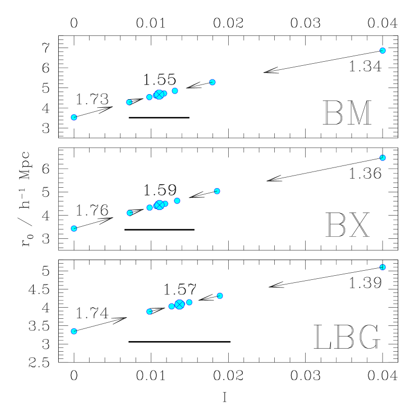
To check the plausibility of our adopted values for ${\cal I}$, we inserted into equation 18 the best power-law fits to $\omega(\theta)$ from each sample’s final iteration. The equation returned $0.008$, $0.006$, and $0.009$ as the empirical estimates of ${\cal I}$ for BM, BX, and LBG samples. These values differ somewhat from the ones we adopt (figure 4), because the empirical and CDM approaches (see 3.1.1) make different assumptions about the behavior of $\omega(\theta)$ on the scales $\theta>200^{\prime\prime}$ where we cannot measure it, but they are consistent within their large $1\sigma$ uncertainties and small changes ($<1\sigma$) to the best-fit values of $\gamma$ would make them agree perfectly. Readers may also be reassured to recall that our estimates of $r_{0}$ and $\gamma$ agree well with those of Porciani & Giavalisco (2002), who corrected for the integral constraint in a completely different way.

We estimated the random uncertainty in $r_{0}$ and $\gamma$ in two ways. First, we analyzed many alternate realizations of our $\omega(\theta)$ measurements that were generated under the assumption that the uncertainties were uncorrelated. To create a single alternate realization, we added to each measured value $\omega(\theta_{i})$ a Gaussian random deviate with standard deviation equal to its uncertainty $\sigma_{i}$. After creating numerous alternate realizations, we calculated and tabulated the values of $r_{0}$ and $\gamma$ implied by each. Our $1\sigma$ confidence interval on $r_{0}$ was defined as the range that contained 68.3% of the measured values of $r_{0}$ among the alternate data sets. The $\gamma$ confidence interval is defined in the same way. We found $r_{0}=4.0\pm 0.2h^{-1}$ Mpc, $\gamma=1.57\pm 0.07$ (LBG), $r_{0}=4.3\pm 0.2h^{-1}$ Mpc, $\gamma=1.59\pm 0.04$ (BX), and $r_{0}=4.7\pm 0.2h^{-1}$ Mpc, $\gamma=1.55\pm 0.06$ (BM). These numbers assume uncorrelated error bars and neglect the uncertainty in our selection functions. The uncertainty in ${\cal I}$ is also neglected, since each alternate realization had the same integral constraint correction.

Our second approach was to extract random subcatalogs from our full galaxy catalog, estimate $r_{0}$ and $\gamma$ for each with the iterative solution for $\omega(\theta)$ described above, measure how the r.m.s. dispersion in best-fit parameter values depended on the number of sources in the subcatalog, and extrapolate to the full catalog size. In fact we created our random subcatalogs in pairs, with both subcatalogs in a pair containing a random fraction $f\leq 0.5$ of the sources in the full catalog and no sources in common between them, and estimated the uncertainty in $r_{0}$ at a given value of $f$ as $2^{-1/2}$ times the r.m.s. difference in $r_{0}$ among pair members. This prevented us from underestimating the random uncertainty in $r_{0}$ as $f\to 0.5$, when random subcatalogs could otherwise contain nearly the same galaxies. With this approach we estimate $r_{0}=4.0\pm 0.5h^{-1}$ Mpc, $\gamma=1.57\pm 0.12$ (LBG), $r_{0}=4.3\pm 0.3h^{-1}$ Mpc, $\gamma=1.59\pm 0.05$ (BX), and $r_{0}=4.7\pm 0.5h^{-1}$ Mpc, $\gamma=1.55\pm 0.07$ (BM). These numbers neglect the uncertainty in our selection function and do not fully account for the uncertainty in ${\cal I}$. They do not assume uncorrelated error bars, however, and we will therefore assume that they are more accurate than the numbers from the preceding paragraph.

The uncertainty in ${\cal I}$ is not negligible. According to equation 15 the $1\sigma$ uncertainty in ${\cal I}$ is $\sim 35$–$50$% as large as ${\cal I}$ itself for our 21 fields. As ${\cal I}$ varies over its $1\sigma$ allowed range, the best-fit parameters $r_{0}$ and $\gamma$ change by roughly as much as the uncertainties quoted above. Adding these changes in quadrature to the random uncertainties above, and making the minor corrections for the selection function uncertainties discussed in § 3.1, we arrive at the following estimates: $r_{0}=4.0\pm 0.6h^{-1}$ Mpc, $\gamma=1.57\pm 0.14$ (LBG), $r_{0}=4.2\pm 0.5h^{-1}$ Mpc, $\gamma=1.59\pm 0.08$ (BX), and $r_{0}=4.5\pm 0.6h^{-1}$ Mpc, $\gamma=1.55\pm 0.10$ (BM).

Other investigators (e.g., Giavalisco & Dickinson 2001; Foucaud et al. 2003) have claimed that at redshift $z\sim 3$ bright galaxies cluster more strongly than faint galaxies. Our data support this conclusion. Figure 5 shows that in the BX and LBG samples the correlation lengths of galaxies with $23.5<{\cal R}<24.75$ ($r_{0}\sim 5.0h^{-1}$ Mpc) exceed those of galaxies with $24.75<{\cal R}<25.5$ ($r_{0}\sim 3.7h^{-1}$ Mpc) by a significant amount. If we split the BX and LBG samples into two halves at random, rather than by apparent magnitude, the difference in correlation lengths between the two halves is this large only about $5$% (BX) to $24$% (LBG) of the time. The situation is less clear for the BM sample at $z\sim 1.7$, where the uncertainties are larger owing to the poor determination of $N(z)$ from the small number of measured redshifts, but the data do not seem to suggest stronger clustering for brighter galaxies. On the one hand it makes sense that UV-brightness should become less associated with strong clustering as redshift decreases, since UV-bright galaxies are known to be weakly clustered at $z=0$ and $z=1$. On the other, the overall clustering of the BM sample is still quite strong, stronger than one expects for typical collapsed objects at $z\sim 1.7$ (see below), and so it seems that the numerous objects too faint to satisfy our selection criteria must be less clustered than the bright objects in our sample. We will wait for additional spectroscopic observations of BM galaxies before commenting further.

Figure 5.— Correlation length $r_{0}$ for bright and faint subsamples of the BM, BX, and LBG samples.

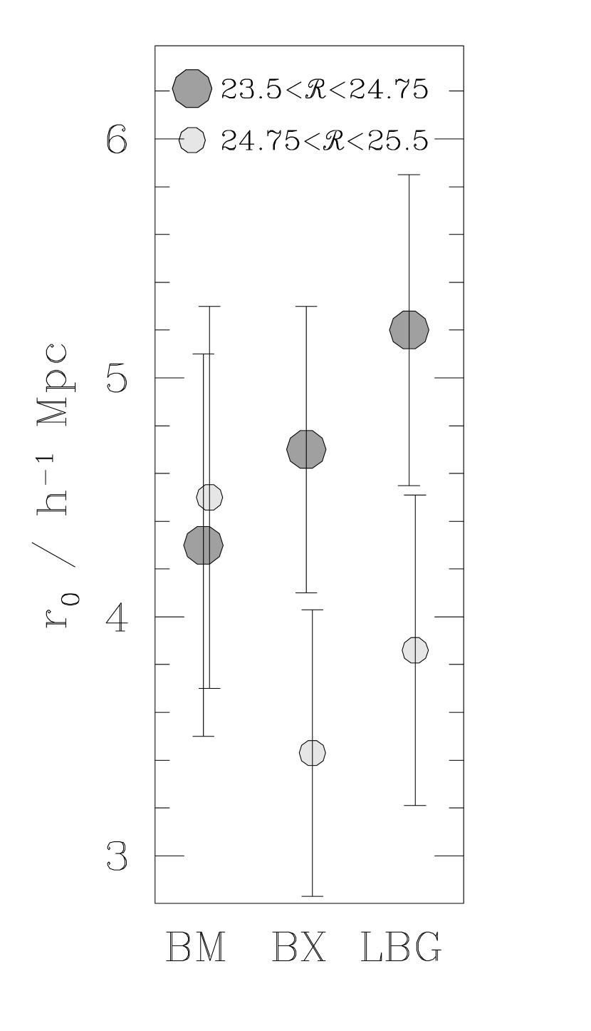
The dependence of clustering strength on luminosity can produce a false impression of a change in $r_{0}$ with redshift, since lower redshift samples will tend to reach fainter absolute luminosities. Truncating the samples at a fixed absolute luminosity does not seem a good solution to us, however, since the bright end of the UV luminosity function rises rapidly towards higher redshifts (e.g., Adelberger & Steidel 2000) and one would therefore be comparing rare objects at lower redshifts to common objects at higher redshifts. A better approach is to compare galaxy samples of roughly the same comoving number density. Since selection with a constant apparent magnitude limit ${\cal R}<25.5$ happens to produce similar comoving number densities for the three samples (see equations 37 and 38 and the related discussion), we will continue to use the constant apparent magnitude limits of equation 1 for our samples in the remainder of the paper. Readers should be aware that the reported value of each sample’s correlation length is somewhat arbitrary for this reason. It reflects the characteristics of the sample as defined here, not of the general galaxy population at high redshift.

4.2. Redshift

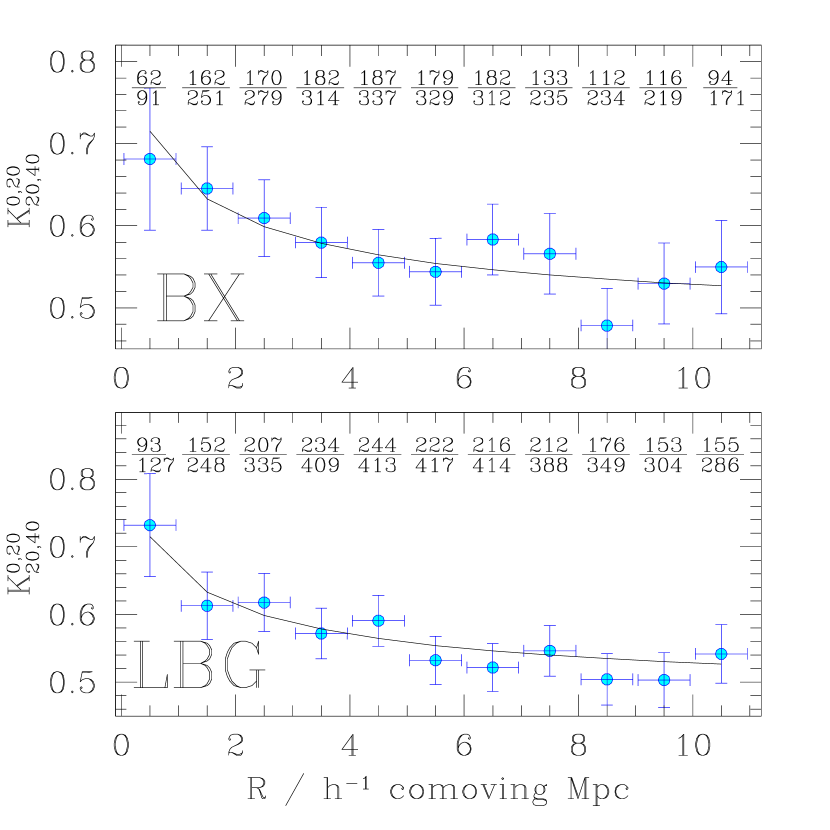
For our estimator of the redshift clustering strength we took $K^{0,20}_{20,40}$, the ratio of the number of galaxy pairs with comoving radial separation $0<|Z|/(h^{-1}{\rm Mpc})<20$ to those with comoving radial separation $0<|Z|/(h^{-1}{\rm Mpc})<40$. Since $20h^{-1}$ Mpc is significantly larger than the uncertainty in each galaxy’s radial position ($\sigma_{Z}\simeq 300\,{\rm km}{\rm s}^{-1}(1+z)/H(z)\sim 3h^{-1}$ comoving Mpc), and since $40h^{-1}$ Mpc is significantly smaller than the selection functions’ widths ($\sigma_{\rm sel}>200h^{-1}$ comoving Mpc), the expected value of $K^{0,20}_{20,40}$ should be given by equation 33. We limited our analysis to pairs with transverse separations $\theta_{ij}<300^{\prime\prime}$, equivalent to $R_{ij}\lower 2.15277pt\hbox{$\;\buildrel<\over{\sim}\;$}5.9h^{-1}$ comoving Mpc at $z=2.5$, to reduce the sensitivity of our results to any deviations of the correlation function from a $\gamma=1.55$ power-law on large scales.

Only the BX and LBG spectroscopic samples were large enough to allow meaningful measurements of $K^{0,20}_{20,40}$. For $\gamma=1.55$, the right-hand side of equation 33 is equal to the observed ratio $K^{0,20}_{20,40}$ when $r_{0}=4.6h^{-1}$ (LBG) or $4.5h^{-1}$ (BX) comoving Mpc. The values change by roughly $\pm 2$% as $\gamma$ is varied from 1.45 to 1.65. When analyzed with this technique, mock galaxy catalogs from the GIF simulation (§ 2.2) with sizes similar to our observed catalogs show a $\pm 1\sigma$ dispersion in $r_{0}$ around the true mean of $0.6h^{-1}$ (LBG) and $0.9h^{-1}$ (BX) comoving Mpc, so we adopt $4.6\pm 0.6h^{-1}$ and $4.5\pm 0.9h^{-1}$ Mpc as the best fit values to $r_{0}$ for our spectroscopic catalogs. The results do not change significantly if we eliminate pairs with $\theta_{ij}<60^{\prime\prime}$ from the analysis, showing that we have measured genuine large-scale clustering and not merely the clumping of objects within individual halos.

Figure 6 presents the result in a more graphical way. We divided our lists of galaxy pairs into bins according to transverse separation $R_{ij}$, then calculated $K^{0,20}_{20,40}$ separately for each bin. Points with error bars show the values we found. The solid lines show the values predicted by the $\gamma=1.55$ correlation function described in the preceding paragraph. The plot shows that the derived correlation function parameters provide a reasonable fit to the clustering of the galaxies in the spectroscopic sample.

Figure 6.— Redshift clustering in the BX and LBG samples. The ordinate shows $K_{20,40}^{0,20}$, the fraction of galaxy pairs with comoving radial separation $0<Z<40h^{-1}$ Mpc that have $0<Z<20h^{-1}$ Mpc. $K_{20,40}^{0,20}$ was calculated for galaxy pairs in different bins of transverse separation $R$. In the absence of clustering $K_{20,40}^{0,20}$ would be equal to $0.5$, on average, at all values of $R$. Instead our data (points with error bars) show that $K_{20,40}^{0,20}$ is generally larger than $0.5$, especially at smaller $R$. This implies a positive correlation function that rises towards smaller separations. The fractions at the top of the plots show the number of galaxies with $0<Z<20h^{-1}$ Mpc and $0<Z<40h^{-1}$ Mpc in each bin of $R$. The error bars are equal to $n^{1/2}/d$ where $n$ is the numerator and $d$ the denominator in the fraction. They are only approximate; the actual analysis treated uncertainties as described in the text. The solid line shows the values of $K_{20,40}^{0,20}$ implied by the best fit of a power-law correlation function $\xi(r)=(r/r_{0})^{-1.55}$ to the data when they are placed in a single radial bin.

4.3. Summary

We presented two independent estimates of the correlation function for each of our galaxy samples. The estimates were consistent with each other, but the first, based on the galaxies’ angular clustering, had somewhat smaller uncertainties. This resulted from the larger size of the photometric sample, and was accentuated by the serious systematics in the spectroscopic sample that made us throw much of our data away. We will adopt the angular clustering results for the remainder of the paper.

5. IMPLICATIONS

5.1. Correspondence to halos

On small scales, smaller than roughly the typical radius $r_{\rm vir}$ of a virialized halo, the spatial clustering of galaxies is difficult to predict or interpret. It depends on the ease with which nearby galaxies merge with each other, on the ability of a galaxy to maintain its star-formation rate as it orbits within a larger potential well, on the possible impact of a galaxy’s feed-back on its surroundings, and so on. On larger scales these baryonic complications have little effect and the correlation function of galaxies should be virtually identical to the correlation function of the halos that host them. To see that this is true, consider the galaxy correlation function in a simplified situation where every galaxy is associated with a single halo and the probability that a galaxy lies a distance $r$ from its halo’s center is $f(r)$. In this case the galaxy distribution will be a Poisson realization of the continuous density field $\rho_{g}({\mathbf{r}})$ that is created when the discrete halo distribution is convolved by $f$, and the galaxy correlation function $\xi_{g}$ will be equal to the correlation function of $\rho_{g}$ (see, e.g., Peebles 1980, eq. 33.6). Since the halo powerspectrum is $P_{h}({\mathbf{k}})=1/n+\int d^{3}r\xi_{h}\exp(i{\mathbf{k}}\cdot{\mathbf{r}})$ (Peebles 1980, eq. 41.5), where $\xi_{h}$ is the halo correlation function and $n$ is the halo number density, since the powerspectrum of $\rho_{g}$ is equal to $|\tilde{f}({\mathbf{k}})|^{2}P_{h}({\mathbf{k}})$, where $\tilde{f}$ is the Fourier transform of $f$, and since the powerspectrum and correlation function are Fourier-transform pairs, the galaxy and halo correlation functions will be related through

$$\xi_{g}({\mathbf{r}})=F({\mathbf{r}})/n+F({\mathbf{r}})\otimes\xi_{h}({\mathbf{r}})$$ (35)

where $\otimes$ denotes convolution and $F\equiv f\otimes f$. Now $f(r)=0$ when $r$ is greater than some maximum separation $r_{\rm max}\sim r_{\rm vir}$; galaxies cannot be located arbitrarily far from the center of their halo. The first term will therefore be zero for $r\gg 2r_{\rm vir}$. The second term will be almost exactly equal to $\xi_{h}(r)$ at the same large separations, because plausible correlation functions do not not change significantly from $r$ to $r+2r_{\rm vir}$ when $r_{\rm vir}\ll r$. This shows that $\xi_{g}(r)\simeq\xi_{h}(r)$ for large $r$. Although it was derived for a simplistic model, the result is more general. As long as galaxies are associated in some way with dark matter halos, and as long as there is some maximum separation $r_{\rm max}\sim r_{\rm vir}$ between each galaxy and the center of its halo, galaxies will have the same correlation function as the halos that host them for $r\gg r_{\rm vir}$. We will accordingly focus our attention solely on separations $r\lower 2.15277pt\hbox{$\;\buildrel>\over{\sim}\;$}1h^{-1}$ comoving Mpc that are many times larger than the typical virial radius.

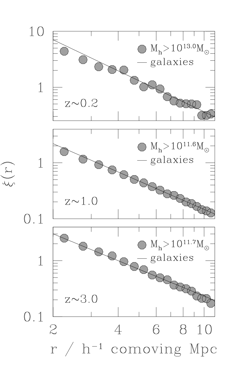
Readers who are skeptical of the claimed similarity between galaxy and halo correlation functions at $r\gg r_{\rm vir}$ may wish to consider figure 7, which compares observed galaxy correlation functions at redshifts $z=0.2$, $1.0$, $3.0$ to the halo correlation functions in the GIF-LCDM simulation outputs at the same redshifts (see § 2.2). The agreement is excellent.

Figure 7.— Comparison of observed galaxy correlation functions to the expected correlation functions of dark matter halos. Solid lines show the power-law fits implied by the parameters reported by Budavári et al. (2003; $r_{0}=5.77\pm 0.09$, $\gamma=1.84\pm 0.02$, $z\simeq 0.2$), by Coil et al. (2003; $r_{0}=3.19\pm 0.51$, $\gamma=1.68\pm 0.07$, $z\simeq 1.0$), and by us (§ 4, $z\simeq 3.0$). In each sample the galaxies’ clustering was measured out to a maximum transverse separation of roughly $10h^{-1}$ comoving Mpc. Circles show the correlation function of halos in the LCDM-GIF simulation (see § 2.2). The halo correlation functions were calculated at the redshift indicated in each panel, and only halos with masses larger than the indicated threshold were included. The comparatively small number of halos with $M>10^{13}M_{\odot}$ is responsible for the noisier halo correlation function at $z=0.2$. In general the agreement between the galaxy and halo correlation functions is excellent, although differences between the galaxy and halo correlation functions arise as $r\to 2h^{-1}$ Mpc and $z\to 0$ because $r$ is no longer enormous compared to the halo radius.

The implied association of galaxies with massive potential wells is hardly surprising. The interesting result is the characteristic mass of the virialized halos that contain the galaxies. This can be estimated since more massive halos cluster more strongly. Figure 8 compares the correlation functions at $1\lower 2.15277pt\hbox{$\;\buildrel<\over{\sim}\;$}r/(h^{-1}{\rm comoving\ Mpc})\lower 2.15277pt\hbox{$\;\buildrel<\over{\sim}\;$}10$ for galaxies in the BM, BX, and LBG samples to the correlation functions of virialized dark matter halos above various mass thresholds in the GIF-LCDM simulation (see § 2.2). The agreement is best if galaxies in the BM, BX, and LBG samples are associated with halos of mass $M\sim 10^{12.1}M_{\odot}$, $10^{12.0}M_{\odot}$, and $10^{11.5}M_{\odot}$, respectively.

Figure 8.— Our best correlation function fits (solid lines) compared to the correlation functions of virialized dark matter halos in the GIF simulation. The halo correlation functions were calculated for halos with mass $M>10^{11.4}M_{\odot}$, $M>10^{12.0}M_{\odot}$, and $M>10^{12.6}M_{\odot}$ that were identified at redshifts $z=1.77$ (BM), $2.32$ (BX), and $2.97$ (LBG). The dependence of halo clustering strength on mass allows one to estimate characteristic masses of the halos that are associated with the galaxies in our samples.

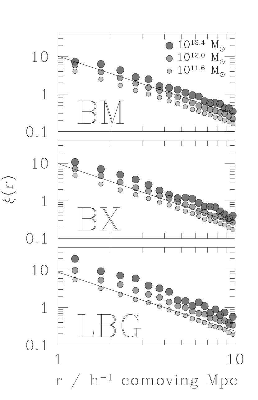
Uncertainties in our measured correlation functions lead to uncertainties in the estimated characteristic masses. The size of these uncertainties can be gauged most cleanly by comparing our measured angular correlation function to the angular correlation functions of halos above different mass thresholds. We calculated halo angular correlation functions numerically from equation 6 after substituting in the observed redshift distributions for the different samples (fig. 1) and the GIF-LCDM halo correlation functions at the mean redshift of each sample. Typical results are shown in figure 9. The halo angular correlation functions fall significantly below the data on small scales, since (by definition) a halo cannot have another halo as a neighbor within the radius $r_{\rm vir}$. As argued above, however, it is the larger scales $r\lower 2.15277pt\hbox{$\;\buildrel>\over{\sim}\;$}1h^{-1}$ comoving Mpc (i.e., $\theta\lower 2.15277pt\hbox{$\;\buildrel>\over{\sim}\;$}1^{\prime}$) that are relevant for comparing to galaxies, and here the agreement is good. The uncertainty in the galaxies’ implied mass scale is dominated by the uncertainty in the integral constraint correction ${\cal I}$ that was applied to the data, since this moves all points up or down together. Rough $1\sigma$ limits on the threshold masses of the hosting halos are

$$10^{11.9} \lower 2.15277pt\hbox{$\;\buildrel<\over{\sim}\;$}M/M_{\odot}\lower 2.15277pt\hbox{$\;\buildrel<\over{\sim}\;$} 10^{12.3}\quad\quad{\rm BM}$$

$$10^{11.8} \lower 2.15277pt\hbox{$\;\buildrel<\over{\sim}\;$}M/M_{\odot}\lower 2.15277pt\hbox{$\;\buildrel<\over{\sim}\;$} 10^{12.2}\quad\quad{\rm BX}$$ (36)

$$10^{11.2} \lower 2.15277pt\hbox{$\;\buildrel<\over{\sim}\;$}M/M_{\odot}\lower 2.15277pt\hbox{$\;\buildrel<\over{\sim}\;$} 10^{11.8}\quad\quad{\rm LBG}.$$

Readers unfamiliar with the idea of threshold masses may wish to see footnote 6 in §6, below, for further discussion of how to interpret them.

Figure 9.— Observed galaxy angular correlation functions compared to the angular correlation functions of halos in the GIF-LCDM simulation. Points with error bars show our observations, including integral constraint correction ${\cal I}\sim 0.01$. (Figure 4 shows the precise values of ${\cal I}$ that were adopted.) Solid lines show the halo angular correlation functions for GIF-LCDM halos of mass $M=10^{11.9}$, $10^{12.3}M_{\odot}$ at the identification redshift $z=1.77$ (BM), of mass $M=10^{11.8}$, $10^{12.2}M_{\odot}$ at the identification redshift $z=2.32$ (BX), and of mass $M=10^{11.2}$, $10^{11.8}M_{\odot}$ at the identification redshift $z=2.97$ (LBG). The angular correlation functions were calculated for the redshift distributions shown in figure 1. In each case the curves for the more massive halo are on top. The plateau in the halo angular clustering at small radii results from the definition of a halo, which imposes a minimum separation for halo neighbors by counting two halos as the same object if they lie too close together. Dotted lines show the angular correlation functions that result when the power-law fits to the three-dimensional halo correlation functions at $2<r<10h^{-1}$ comoving Mpc are extrapolated to $r=0$. They are for reference only; the galaxy and halo angular correlation functions should be compared only at the separations $\theta\lower 2.15277pt\hbox{$\;\buildrel>\over{\sim}\;$}60^{\prime\prime}$ where they are expected to be similar (see equation 35). The two halo curves in each panel roughly span the range in angular clustering strength allowed by the uncertainty of $\sim 0.005$ in ${\cal I}$, and so the masses of the halos listed above should roughly bracket the allowed masses of the halos that host the galaxies.

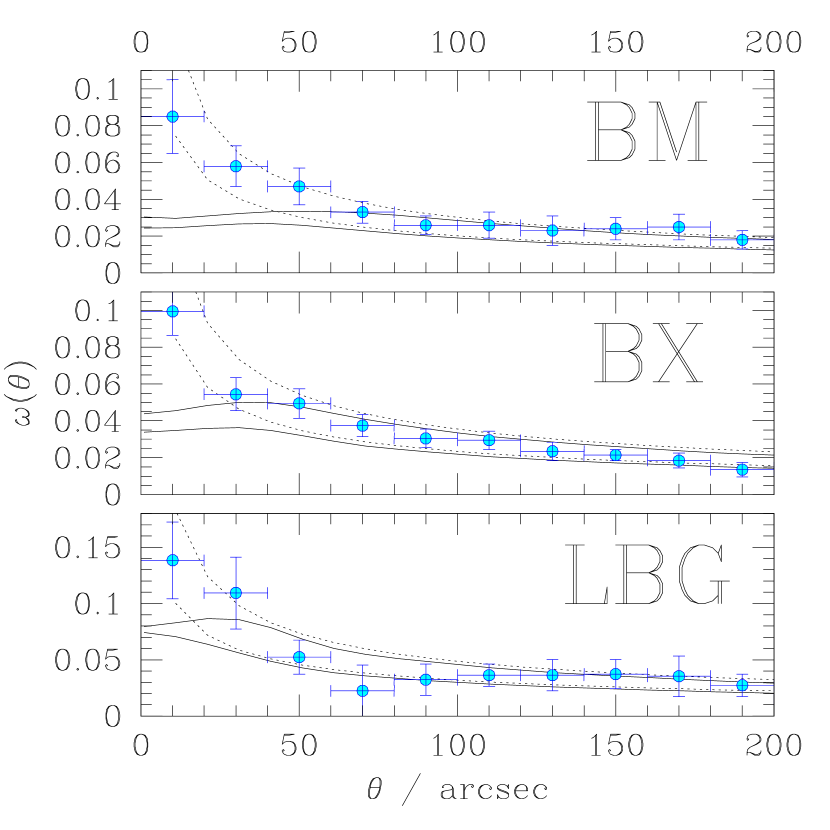
One implication of figure 9 is that some halos are occupied by more than one of the galaxies in our samples; the data on small scales are strongly inconsistent with the correlation functions that assumed one object per halo. (This was first pointed out by Wechsler et al. (2001) and later denied by Porciani & Giavalisco (2002). Our analysis agrees far better with that of Wechsler et al.) The fraction of LBGs that reside in the same halo as another LBG can be calculated as follows. If there were never more than one LBG per halo, the expected number of LBGs within $1^{\prime}$ of a randomly chosen LBG would be $N_{1}={\cal N}(1+\bar{\omega}_{1})$ where ${\cal N}$ is the surface density of LBGs, $\bar{\omega}_{1}\equiv\int_{0}^{1^{\prime}}\theta d\theta\,\omega_{h}(\theta)/\int_{0}^{1^{\prime}}\theta d\theta$, and $\omega_{h}$ is halo angular correlation function that fits our data best for $\theta>1^{\prime}$. The actual number of LBGs within $1^{\prime}$, $N_{\rm true}$, is given by the same equation with the halo correlation function $\omega_{h}$ replaced by the galaxy correlation function $\omega_{\rm true}$. The expected number of additional LBGs in a halo that is known to contain one LBG, $f_{\rm LBG}$, is equal to the difference between $N_{\rm true}$ and $N_{1}$. Numerically integrating the angular correlation functions for observed galaxies and simulated halos, and multiplying by the LBG surface density from table 1, we estimate $f_{\rm LBG}\sim 0.05$. The numbers for the other samples, estimated with a similar approach, are $f_{\rm BX}\sim 0.25$ and $f_{\rm BM}\sim 0.25$. Some galaxies must share the same halo to explain the data, but the required number is small. Note that we are referring solely to galaxies that satisfy our color and magnitude selection criteria; we obviously cannot say anything about the spatial distribution of galaxies that are not in our samples.

Having established a rough characteristic mass for the halos that contain our galaxies, we can compare the galaxy and halo number densities and estimate what fraction of the most massive halos at redshifts $1.5\lower 2.15277pt\hbox{$\;\buildrel<\over{\sim}\;$}z\lower 2.15277pt\hbox{$\;\buildrel<\over{\sim}\;$}3.5$ do not contain a galaxy that is detectable with our techniques. According to Adelberger & Steidel (2000) the comoving number density of LBGs brighter than ${\cal R}=25.5$ is

$$n_{\rm LBG}=(4\pm 2)\times 10^{-3}h^{3}{\rm Mpc}^{-3}$$ (37)

for $\Omega_{M}=0.3$, $\Omega_{\Lambda}=0.7$. Combining the BM and BX completeness coefficients in table 3 of Adelberger et al. (2004) with the surface densities in table 1 of this paper, we estimate

$$n_{\rm BX} = (6\pm 3)\times 10^{-3}h^{3}{\rm Mpc}^{-3}$$

$$n_{\rm BM} = (5\pm 2.5)\times 10^{-3}h^{3}{\rm Mpc}^{-3}$$ (38)

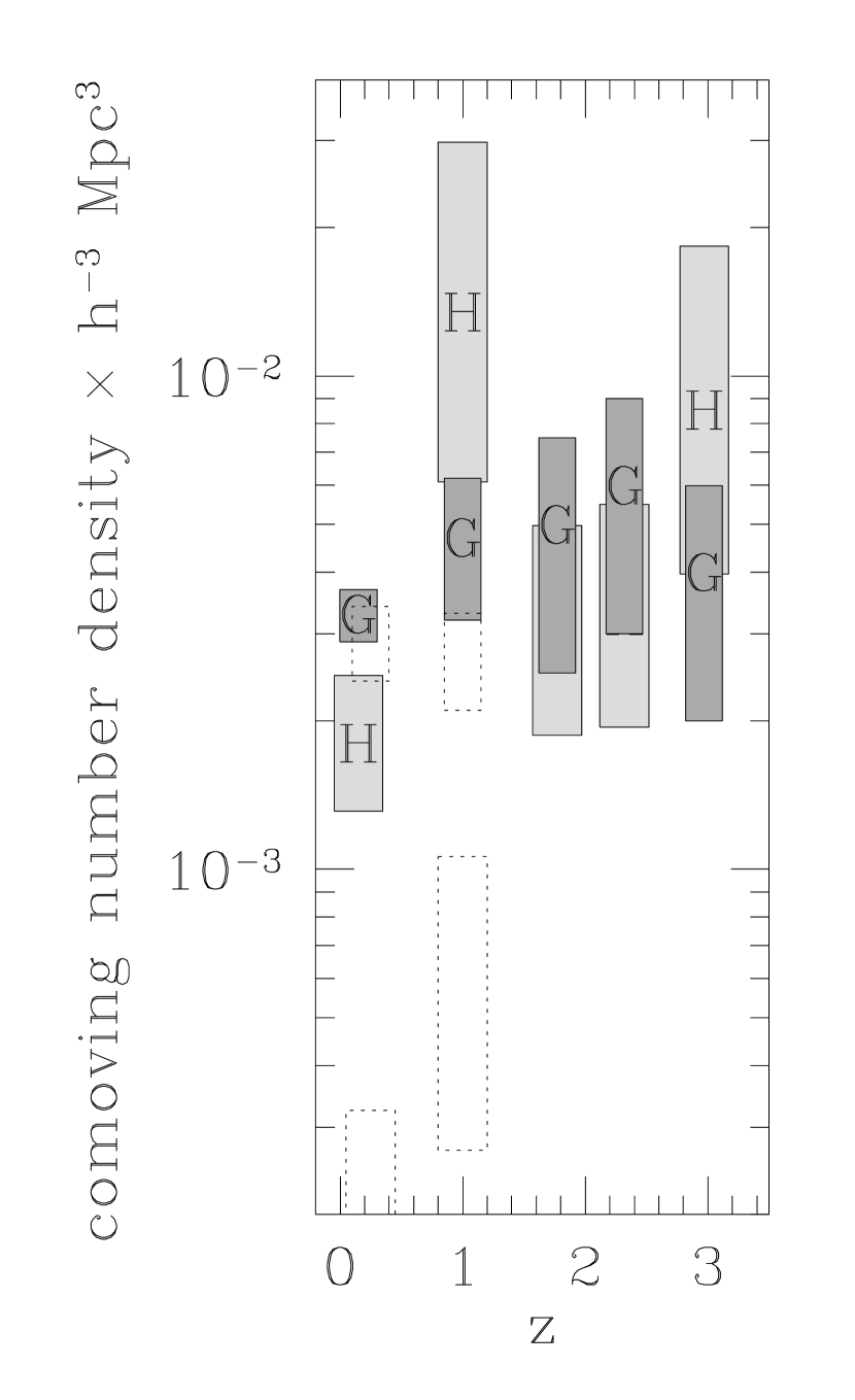
where the assigned uncertainties of 50% are approximate guesses that will be refined later with Monte Carlo simulations. Number densities for the population of halos that contain the galaxies can be estimated from the GIF-LCDM simulation given the range of halo masses (equation 5.1) that are compatible with the galaxies’ clustering strength. Figure 10 shows that the number density of galaxies in the BM, BX, and LBG samples is comparable to the number density of halos that can host them. As we will discuss in § 6, below, this implies that the duty cycle of star-formation in the galaxies must be of order unity and shows that our surveys cannot be severely incomplete. Similar arguments have been made by Adelberger et al. (1998), Giavalisco & Dickinson (2000), Martini & Weinberg (2001), and others.

Figure 10.— The comoving number densities of galaxies (G) in various samples compared to the comoving number density of the halos (H) at the same redshift that have the same clustering strength (on large scales) as the galaxies. These are the halos that the galaxies can reside within. Shaded regions are for star-forming galaxies and their associated halos: the “blue” SDSS sample of Budavári et al. (2003; $z=0.2$), the emission-line sample of Coil et al. (2004; $z=1$), and our three samples ($z>1.5$). The height of the rectangles covers the $\pm 1\sigma$ range in number density. The uncertainties in halo number density follow from the uncertainty in their galaxy’s clustering strength. At each redshift star-forming galaxies are roughly as numerous as the halos that can host them. Galaxies that are no longer forming stars tend to outnumber halos with similar clustering strength, which shows that several reside in the same halo. This is evident in both the absorption-line sample of Coil et al. (2004; dotted rectangles at $z=1$) and the elliptical sample of Budavári et al. (2003; $-23<M_{r}<-21$, dotted rectangles at $z=0.2$). For consistency with the Budavári sample, the number density of early-type galaxies at $z\sim 1$ was calculated by integrating the $z\sim 1$ early-type luminosity function of Chen et al. (2003) over all magnitudes brighter than $M_{R}=-21$.

5.2. Evolution

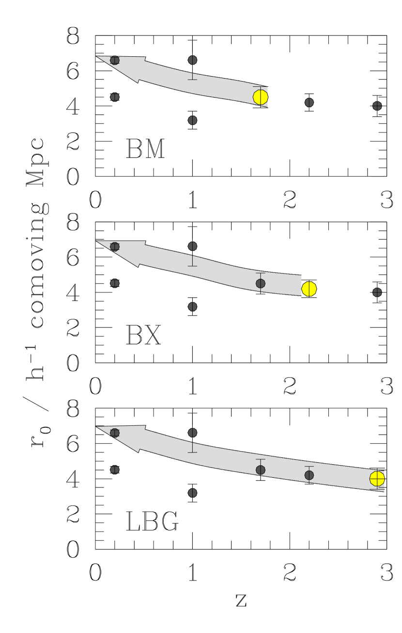
The spatial distribution of a population of galaxies evolves in an easily predictable way as it responds to the gravitational pull of dark matter. We used a simple approach to estimate this evolution from the LCDM-GIF simulation. After connecting the observed galaxies to halos with a range of masses (equation 5.1), we measured the evolution in the clustering of those halos in the simulation and assumed that the galaxies’ clustering would evolve in the same way. See § 2.2. Figure 11 shows the implied change in correlation length $r_{0}$ with time for the galaxies in our samples. By $z\sim 2$ galaxies in the LBG sample will have a correlation length similar to measured correlation lengths of galaxies in the BM and BX samples. By $z\sim 1$ their correlation length will be similar to the correlation length of early-type (i.e., “absorption line”) galaxies in the sample of Coil et al. (2003). By $z\sim 0.2$ their correlation length will be equal to the observed correlation length of ellipticals (Budavári et al. 2003). The evolution of $r_{0}$ for galaxies in the BM and BX samples is similar.

Figure 11.— Clustering strength versus redshift. Top panel: the large, lightly shaded point shows the correlation length we infer for galaxies in the BM sample. The arrow shows the correlation length these galaxies will have at lower redshifts. The top edge of the arrow shows the evolution of $r_{0}$ for halos in the LCDM-GIF simulation that had mass exceeding $M_{\rm top}=10^{12.3}M_{\odot}$ at the redshift of identification $z_{\rm id}=1.77$; the bottom edge is for halos with mass exceeding $M_{\rm bot}=10^{11.9}M_{\odot}$. Smaller, darker points show measurements of $r_{0}$ from other samples: the SDSS “elliptical” and blue samples of Budavári et al. (2003; $z=0.2$ and $r_{0}=6.6$, $4.5$ respectively), the DEEP full and absorption-line samples of Coil et al. (2003; $z=1$ and $r_{0}=3.2$, $6.6$ respectively), and the BX and LBG samples of this paper. Middle panel: similar to the top panel, except $z_{\rm id}=2.32$, $M_{\rm top}=10^{12.2}M_{\odot}$, $M_{\rm bot}=10^{11.8}M_{\odot}$, and the large point is for the BX sample. Bottom panel: similar to the top panel, except $z_{\rm id}=2.97$, $M_{\rm top}=10^{11.8}M_{\odot}$, $M_{\rm bot}=10^{11.2}M_{\odot}$, and the large point is for the LBG sample.

Figures 12 and 13 present a more detailed view of the possible relationships between the descendants of galaxies in our samples and various galaxy populations at lower redshift. Figure 12 shows that at $z=1$ the descendants’ clustering strength will significantly exceed that of average galaxies in optical magnitude-limited surveys. Since these surveys are dominated by star-forming (“emission-line”) galaxies, we can conclude that the typical descendant is no longer forming stars by $z\sim 1$. A similar point was made by Adelberger (2000) and Coil et al. (2004). The stronger clustering of redder and brighter sub-populations at $z\sim 1$ is more compatible with the descendants’ expected clustering, but the match is best for the sub-population with early-type spectra. This is especially true for descendants of the brightest galaxies in the BX and LBG samples. Although the observed number density of early-type galaxies at redshift $z\sim 1$, roughly $(7\pm 1.5)\times 10^{-3}h^{3}{\rm Mpc}^{-3}$ (Chen et al. 2003), is consistent with the idea that most had a BM/BX/LBG galaxy as a progenitor, we cannot rule out the idea that some had multiple merged BM/BX/LBG progenitors and others had none.

Figure 12.— Clustering strength of LBG descendants and of different galaxy populations in the $z\sim 1$ DEEP optically selected sample of Coil et al. (2003). Galaxies at $z\sim 1$ that are brighter ($M_{B}<-19.75$), that are redder in observed $R-I$ or rest-frame $(B-R)_{0}$, or that have early-type (absorption line) spectra cluster more strongly than star-forming (emission line) galaxies or than galaxies in the full sample (“All”). The shaded regions in the background show the range of correlation length at $z=1$ expected for descendants of typical ($23.5<{\cal R}<25.5$) and bright ($23.5<{\cal R}<24.75$) LBGs. The correlation lengths are similar for descendants of BX and BM galaxies (see figure 11). The galaxies at $z\sim 1$ that cluster strongly enough to be descended from BM, BX, or LBG galaxies have early type spectra and are red.

Figure 13.— Correlation length and number density of LBG descendants and of different galaxy populations in the SDSS sample of Budavári et al. (2003). The darker shaded region in the background shows the range of clustering strength at $z=0.2$ expected for the descendants of typical LBGs ($23.5<{\cal R}<25.5$) and the observed number density of typical LBGs at $z\sim 3$. The lighter shaded region above and to the left is for bright LBGs ($23.5<{\cal R}<24.75$). Values for BX and BM descendants are similar (see figure 11 and equations 37 and 38). Points show measured values for galaxy populations at $z\sim 0.2$. The descriptive labels on the points correspond to the sub-samples defined by Budavári et al. (2003) as follows: All $\to$ full sample; bright $\to$ $-21>M_{r}>-22$; brightest $\to$ $-22>M_{r}>-23$; normal blue $\to$ $M_{r}>-21$, $t>0.65$; bright blue $\to$ $-21>M_{r}>-23$, $t>0.65$; normal E $\to$ $M_{r}>-21$, $t<0.02$; bright E $\to$ $-21>M_{r}>-23$, $t<0.02$.

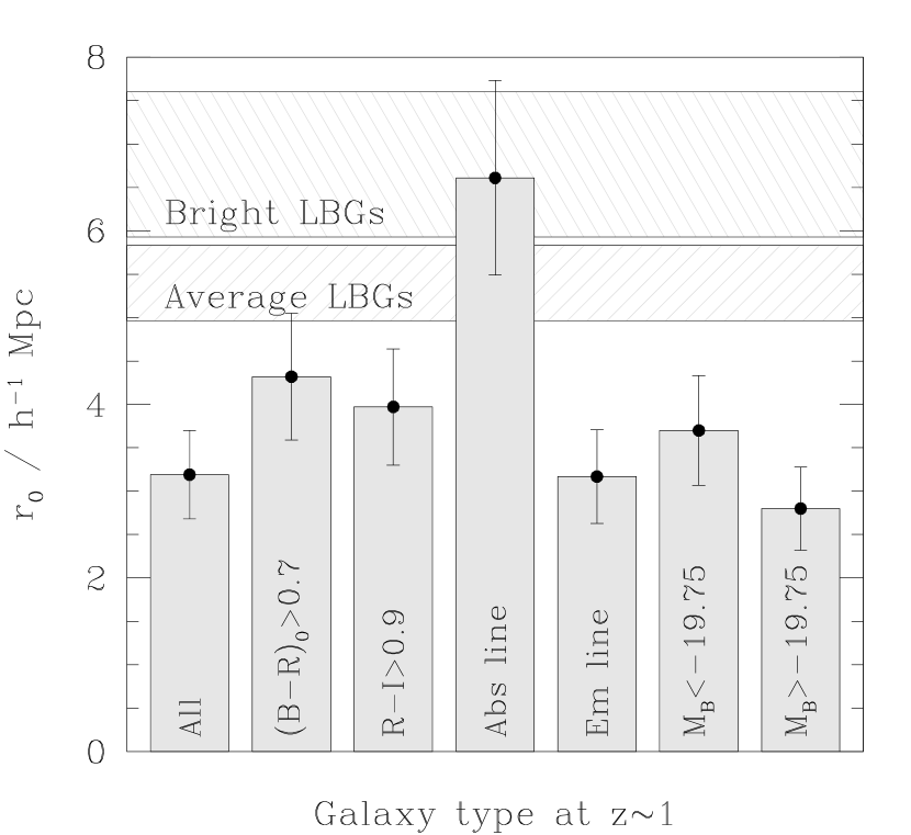
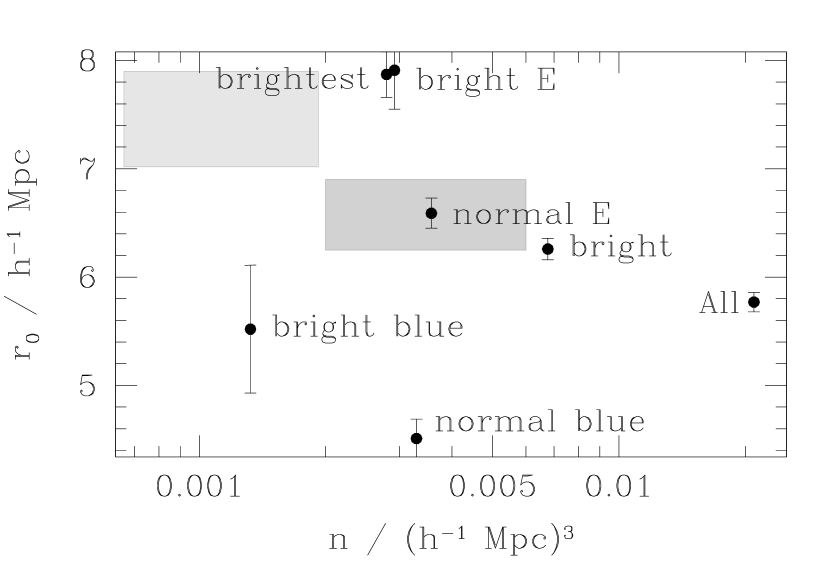
Figure 13 is an analogous plot for redshift $z\sim 0.2$. Correlation lengths for various populations in the Sloan Digital Sky Survey (SDSS) were taken from Budavári et al. (2003). Number densities were calculated assuming a surveyed volume of $10^{8}h^{-3}$ Mpc³ with an uncertainty of $\sim 15$% (T. Budavári 2004, private communication). The expected $z=0.2$ clustering strength of typical LBG descendants (darker shaded box) agrees best with the clustering of galaxies with early-type SEDs in the Budavári et al. (2003) sample. The galaxies in our high-redshift samples are roughly as numerous as these early-type galaxies, though the possibility of merging prevents us from estimating the number density of their BM/BX/LBG descendants at $z\sim 0.2$. The descendants of brighter LBGs will have a correlation length closer to that of bright ellipticals, though there are probably not enough descendants to account for the entire bright elliptical population.

6. SUMMARY & DISCUSSION

The first part of the paper was concerned with measuring the spatial clustering of large samples of star-forming galaxies at redshifts $z\sim 1.7$, $2.2$, and $2.9$. We fit a three-dimensional correlation of the form $\xi(r)=(r/r_{0})^{-\gamma}$ to the galaxies’ angular clustering with standard techniques and to the galaxies’ redshift clustering with a new estimator. The new estimator, $K$, is insensitive to many of the possible systematic biases in our spectroscopic surveys. We reached consistent conclusions about the correlation function with the two approaches, but adopted the angular results since their random uncertainties were somewhat smaller. As given in § 4.1, the best-fit correlation-function parameters from the angular clustering are

$$r_{0}/(h^{-1}{\rm Mpc}),\gamma=\cases{4.0\pm 0.6,1.57\pm 0.14&LBG\cr 4.2\pm 0.5,1.59\pm 0.08&BX\cr 4.5\pm 0.6,1.55\pm 0.10&BM\cr}$$ (39)

where BM, BX, and LBG are the names we have given the $U_{n}G{\cal R}$ color-selection criteria that we used to find galaxies at $z\sim 1.7$, $2.2$, and $2.9$ (§ 2.1). The quoted $1\sigma$ errors include random uncertainties, uncertainties in the integral constraint corrections, and uncertainties in the shapes of the selection functions.

Since the value of $r_{0}$ depends on the apparent-magnitude limit of the samples, at least in the two higher-redshift bins (figure 5), the reported values of $r_{0}$ are somewhat arbitrary. We chose to limit each sample to a fixed range of apparent magnitudes, $23.5<{\cal R}<25.5$, on the grounds that this resulted in a similar comoving density in each redshift bin. Different magnitude limits would have resulted in different correlation lengths. Readers should be aware that the numbers we give are appropriate to the samples as we have defined them, not to the general galaxy population at high redshifts.

The second part of the paper was based on the proposition that WMAP (Spergel et al. 2003) and other experiments have given us reliable measurements of the cosmological parameters and of the shape of the dark matter power-spectrum. This implies that we know what sorts of virialized dark-matter halos existed at different epochs in the past and how their spatial distribution evolved over time. Since galaxies reside within dark-matter halos, they will have the same correlation function as the halos on large scales (equation 35). The galaxies’ clustering should therefore tell us what sort of halo they reside within. We found a good match (figures 8 and 9) between the correlation functions of the galaxies and of halos with threshold masses ranging from $10^{11.5}M_{\odot}$ (LBG) to $10^{12.1}M_{\odot}$ (BM). Equation 5.1 gives rough $1\sigma$ limits on the halos’ total masses. Similar masses for Lyman-break galaxies have been derived with the same approach by Jing & Suto (1998), Adelberger et al. (1998), Giavalisco & Dickinson (2000), Porciani & Giavalisco (2002), and others. Although the estimated masses were derived solely from the galaxy clustering, they seem reasonable on other grounds. They cannot be much higher. The number density of halos would be lower than the number density of LBGs, for example, if the halo mass were greater than $10^{11.8}M_{\odot}$. Such large halo masses would be possible only if significantly more than one LBG resided in the typical halo, and that is something that our observations rule out (§ 5.1). Nor can they be much lower. The halos that contain LBGs would not have enough baryons to form the median LBG stellar mass of roughly $10^{10}M_{\odot}$ (Shapley et al. 2001) unless their total mass were greater than about $10^{11}M_{\odot}$.

We should mention in passing that our best-fit halo masses seem to imply that only a small fraction of the baryons in the halos are associated with the observed galaxies. For example, the best-fit mass threshold of $10^{11.5}M_{\odot}$ for LBGs corresponds to a median total mass of $10^{11.86}M_{\odot}$ and median baryonic mass of $1.2\times 10^{11}M_{\odot}$ (for $\Omega_{b}/\Omega_{M}\simeq 0.17$, Spergel et al. 2003), roughly ten times larger than the observed stellar masses of LBGs. Since the $10^{8}$ supernovae that explode during the assembly of the typical LBG’s stellar mass will eject roughly $10^{8}M_{\odot}$ of metals (e.g., Woosley & Weaver 1995), enough to enrich at most $1.3\times 10^{10}M_{\odot}$ of gas to LBGs’ typical metallicities of $0.4Z_{\odot}$ (Pettini et al. 2002), their observed interstellar gas cannot contain a large fraction of the remaining baryons. These baryons need not be associated with other objects in the halo, however. They may be locked in dim stars that formed in previous episodes of star-formation (e.g., Papovich, Dickinson, & Ferguson 2001), or may have been heated by various processes to undetectably high temperatures. The latter is presumably the case for nearby galaxies, whose ratios of mass in stars and gas to total mass are usually also smaller than the WMAP value $\Omega_{b}/\Omega_{M}\simeq 0.17$. The Milky Way, for example, has a total mass of $10^{12}M_{\odot}$ (Zaritsky 1999; Wilkinson & Evans 1999) and a mass in gas and stars of only $\sim 8\times 10^{10}M_{\odot}$ (K. Freeman 2004, private communication), yet few would assert that its missing baryons belong to another galaxy in its halo.

After establishing plausible total masses for the halos associated with the galaxies, we considered some of the implications. Our arguments were not new (see, e.g., Moustakas & Somerville 2002, Martini & Weinberg 2001, Adelberger et al. 1998). They seemed worth revisiting only because our knowledge of the cosmogony, of the local universe, and of high-redshift galaxies has improved so much in the last few years. We began by estimating the completeness of our surveys from a comparison of the galaxies’ number densities to the number densities of halos with similar clustering strength (figure 10). Similar number densities would imply that almost all of the most massive halos contained a galaxy that satisfied our selection criteria; a much lower galaxy number density would imply that most of the galaxies in massive halos are missed by our survey. Defining $\eta$ as the ratio of galaxy to halo number density, we found rough $1\sigma$ limits of $0.2<\eta_{\rm LBG}<1$, $0.6<\eta_{\rm BX}<3$, and $0.5<\eta_{\rm BM}<2.5$. These limits were derived from the clustering at radii $r\lower 2.15277pt\hbox{$\;\buildrel>\over{\sim}\;$}1h^{-1}$ comoving Mpc. The clustering on smaller scales, sensitive to the possible presence of more than one galaxy in a halo, implies that the upper limits on $\eta_{\rm BX}$ and $\eta_{\rm BM}$ should be revised downwards to $\sim 1.25$. The data appear consistent with the claim of Franx et al. (2003) that our selection criteria find roughly half of the most massive galaxies at $z\sim 2$. A completeness of order $50$% seems plausible to us for other reasons as well. Shapley et al. (2001) estimate a lifetime for the typical LBG of $\sim 3\times 10^{8}$ yr, for example, which implies that the typical LBG will be bright enough for us to detect for only about half of the time that elapsed between the survey selection limits of $z\sim 3.4$ and $z\sim 2.6$.

We considered next the way the clustering of the galaxies would evolve (figure 11). Analysis of the GIF-LCDM simulation suggested that the correlation length of LBG descendants would be similar by $z\sim 2.2$ to the correlation length of galaxies in the BX sample and by $z\sim 1.7$ to the correlation length of galaxies in the BM sample. The spatial clustering is therefore consistent with the idea that we are seeing the same population at all three redshifts, though the selection criteria’s $\sim 50$% incompleteness leaves room for the populations to be distinct and the difference in stellar masses between the LBG ($10^{10}M_{\odot}$) and BX ($2\times 10^{10}M_{\odot}$; Steidel et al. 2005, in preparation) samples may not be consistent with continuous star-formation at observed rates through the elapsed time. Turning our attention to lower redshifts, we found that at $z\sim 1$ our descendants’ clustering would most closely match the observed clustering of galaxies that are red and bright and have early-type spectra (figure 12). By $z\sim 0.2$ the estimated clustering of the descendants suggested elliptical galaxies as the most likely counterparts (figure 13). The correspondence is especially hard to dispute for the descendants of the brightest and most strongly clustered galaxies in the high-redshift samples.

One conclusion seems difficult to escape: the descendants of the galaxies in our samples must have significantly larger stellar masses than their high-redshift forebears. Only $\sim 25$% of the total stellar mass in the local universe is found in galaxies with stellar masses smaller than $2\times 10^{10}M_{\odot}$ (Kauffmann et al. 2003), similar to the values in our high-redshift samples, and these faint galaxies are too weakly clustered to have descended from the galaxies we find at $1.4<z<3.5$. Only elliptical galaxies have a spatial distribution consistent with our expectations for the descendants, and the characteristic stellar mass of ellipticals is $10^{11}M_{\odot}$ (Padmanabhan et al. 2004). The increase in stellar mass from $z\sim 2$ to $z\sim 0$ could have been produced by ongoing star formation or by mergers. Our results at redshift $z\sim 1$ may favor the latter, but in any case our findings are strongly inconsistent with traditional notions of monolithic collapse.

It would be unfair to close without mentioning one population of high-redshift galaxies that we have ignored completely. These are the bright ($K\lower 2.15277pt\hbox{$\;\buildrel<\over{\sim}\;$}20$) near-infrared-selected galaxies. Their reported star-formation rates ($\sim 200M_{\odot}$/yr), correlation lengths ($>9h^{-1}$ Mpc, Daddi et al. 2004) and stellar masses ($2\times 10^{11}M_{\odot}$; van Dokkum et al. 2004) are extraordinary, far larger than the corresponding values for typical galaxies in our samples. Galaxies with similarly extreme properties are not a negligible component of the high redshift universe. The shape of the $850\mu$m background implies that up to a third (Cowie, Barger, & Kneib 2002) of all stars could have formed in objects with star-formation rates greater than $\sim 200M_{\odot}$; halos at $z\sim 3$ with the large masses $M\lower 2.15277pt\hbox{$\;\buildrel>\over{\sim}\;$}10^{12.7}M_{\odot}$ implied by $r_{0}\sim 8$–$9h^{-1}$ Mpc contain in total almost $20$% as many baryons as the more numerous and smaller halos with $M\sim 10^{11.5}M_{\odot}$ that contain LBGs; objects with stellar masses $M_{\ast}>2\times 10^{11}M_{\odot}$ contain nearly $5$% of all stars in the local universe (Kauffmann et al. 2003) and $20$% of the stars in local elliptical galaxies (Padmanabhan et al. 2004). No treatment will be entirely complete if it neglects galaxies similar to those found in near-IR surveys. The galaxies we studied are neither the most massive, nor the most rapidly star-forming, nor the most clustered galaxies in the high redshift universe, but it is precisely this that makes them plausible progenitors for the early-type galaxies that surround us today.

We are grateful to the Virgo consortium for its public release of the GIF simulation data and to G. Kauffmann for bringing the data to our attention. A. Coil and T. Budavári responded helpfully to our questions about their data. M. Giavalisco, the referee, gave us an insightful report. KLA, AES, and NAR were supported by fellowships from the Carnegie Institute of Washington, the Miller Foundation, and the National Science Foundation. DKE and CCS were supported by grant AST 03-07263 from the National Science Foundation.

References

- (1) Adelberger, K.L., Steidel, C.C., Giavalisco, M., Dickinson, M., Pettini, M. & Kellogg, M. 1998, ApJ, 505, 18
- (2) Adelberger, K.L. 2000, in “Clustering at High Redshift,” ASP Conf Series 200, eds. Mazure, Le Fèvre, Le Brun, p13
- (3) Adelberger, K.L. & Steidel, C.C. 2000, ApJ, 544, 218
- (4) Adelberger, K.L., Steidel, C.C., Shapley, A.E., Hunt, M.P., Erb, D.K., Reddy, N.A., & Pettini, M. 2004, ApJ, 607, 226
- (5) Adelberger, K.L., Erb, D.K., et al. 2005, ApJ, submitted
- (6) Arnouts, S., Moscardini, L., Vanzella, E., Colombi, S., Cristiani, S., Fontana, A., Giallongo, E., Matarrese, S., & Saracco, P. 2002, MNRAS, 329, 355
- (7)
- (8) Baldry, I.K. & Glazebrook, K. 2003, ApJ, 593, 258
- (9) Budavári, T. et al. 2003, ApJ, 595, 59
- (10) Bullock, J.S., Wechsler, R.H., & Somerville, R.S. 2002, MNRAS, 329, 246
- (11) Chen, H.-W., Marzke, R.O., McCarthy, P.J., Martini, P., Carlberg, R.G., Persson, S.E., Bunker, A., Bridge, C.R., & Abraham, R.G., 2003, ApJ, 586, 745
- (12) Coil, A.L. et al., 2004, ApJ, in press (astro-ph/0305586)
- (13) Cowie, L.L., Barger, A.J., & Kneib, J.-P. 2002, AJ, 123, 2197
- (14) Daddi, E., Röttgering, H.J.A., Labbé, I., Rudnick, G., Franx, M., Moorwood, A.F.M., Rix, H.W., van den Werf, P.P., & van Dokkum, P.G. 2003, ApJ, 588, 50
- (15)
- (16) Foucaud, S., McCracken, H.J., Le Fèvre, O., Arnouts, S., Brodwin, M., Lilly, S.J., Crampton, D., & Mellier, Y. 2003, A& A, 409, 835
- (17) Franx, M. et al. 2003, ApJL, 587, 79
- (18) Giavalisco, M. 2002, ARAA, 40, 579
- (19) Giavalisco, M. & Dickinson, M. 2001, ApJ, 550, 177
- (20) Hamilton, A.J.S. 1993, ApJ, 417, 19
- (21) Infante, L. 1994, A& A, 282, 353
- (22) Jenkins, A., Frenk, C.S., Pearce, F.R., Thomas, P.A., Colberg, J.M., White, S.D.M., Couchman, H.M.P., Peacock, J.A., Efstathiou, G., & Nelson, A.H., 1998, ApJ, 499, 20
- (23) Jing, Y.P. & Suto, Y. 1998, ApJL, 494, L5
- (24) Kauffmann, G., Colberg, J.M., Diafero, A., & White, S.D.M., 1999, MNRAS, 303, 188
- (25) Kauffmann, G. et al. 2003, MNRAS, 341, 33
- (26)
- (27) Landy, S.D. & Szalay, A.S. 1993, ApJ, 412, 64
- (28) Leitherer, C. 1998, in “Dwarf Galaxies and Cosmology,” eds. T.X. Thuan, C. Balkowski, V. Cayatte, & J.T.T. Van (Gif-sur-Yvette: Editions Frontieres), 235
- (29) Martini, P. & Weinberg, D.H. 2001, ApJ, 547, 12
- (30) Moustakas, L.A. & Somerville, R.S. 2002, ApJ, 577, 1
- (31) Oke, J.B. et al. 1995, PASP, 107, 3750
- (32) Ouchi, M. et al. 2001, ApJ, 558, 83
- (33) Padmanabhan, N. et al., 2004, New Astron, 9, 329
- (34) Papovich, C., Dickinson, M., & Ferguson, H.C. 2001, ApJ, 559, 620
- (35) Peebles, P.J.E., 1980, The Large-Scale Structure of the Universe, (Princeton, Princeton University Press)
- (36) Pettini, M., Rix, S.A., Steidel, C.C., Adelberger, K.L., Hunt, M.P., & Shapley, A.E. 2002, ApJ, 569, 742
- (37) Porciani, C. & Giavalisco, M. 2002, ApJ, 565, 24
- (38) Press, W. H., Flannery, B. P., Teukolsky, S. A., & Vetterling, W.T. 1992, “Numerical Recipes in C”, (Cambridge: Cambridge University Press)
- (39) Renzini, A., in “IMF@50: The Initial Mass Function 50 Years Later,” conference proceedings, in press
- (40) Roche, N. & Eales, S.A. 1999, MNRAS, 307, 703
- (41) Shapley, A.E., Steidel, C.C., Adelberger, K.L., Dickinson, M., Giavalisco, M., & Pettini, M. 2001, ApJ, 562, 95
- (42) Shapley, A.E. et al. 2004, ApJ, in press
- (43)
- (44) Spergel, D.N. et al. 2003, ApJS, 148, 175
- (45) Steidel, C.C., Adelberger, K.L., Shapley, A.E., Pettini, M., Dickinson, M., & Giavalisco, M. 2003, ApJ, 592, 728
- (46) Steidel, C.C., Shapley, A.E., Pettini, M., Adelberger, K.L., Erb, D.K., Reddy, N.A., & Hunt, M.P. 2004, ApJ, 604, 534
- (47) Totsuji, H. & Kihara, T. 1969, PASJ, 21, 221
- (48) van Dokkum, P.G. et al. 2004, ApJ, in press (astro-ph/0404471)
- (49)
- (50) Wechsler, R.H., Somerville, R.S., Bullock, J.S., Kolatt, T.S., Primack, J.R., Blumenthal, G.R., & Dekel, A. 2001, ApJ, 554, 85
- (51) Wilkinson, M.I. & Evans, N.W. 1999, MNRAS, 310, 645
- (52) Woosley, S.E. & Weaver, T.A. 1995, ApJS, 101, 181
- (53) Zaritsky, D. 1999, in the Third Stromlo Symposium: The Galactic Halo, eds. B.K. Gibson, T.S. Axelrod, & M.E. Putman, ASP Conf Ser 165, 34