The properties and luminosity function
of extremely low luminosity galaxies

Abstract

We examine a sample of low redshift ($10<d<150$ $h^{-1}$ Mpc) field galaxies including galaxies with luminosities as low as $M_{r}-5\log_{10}h\sim-12.5$, selected from the Sloan Digital Sky Survey Data Release 2 (SDSS). The sample is unique in containing galaxies of extremely low luminosities in a wide range of environments, selected with uniform and well-understood criteria. We present the luminosity function as well as the broad-band properties of low luminosity galaxies in this sample. A Schechter function is an insufficient parameterization of the $r$-band luminosity function; there is an upturn in the slope for $M_{r}-5\log_{10}h>-18$. The resulting slope at low luminosities in this sample is $\alpha_{2}\sim-1.3$. However, we almost certainly miss a large number of galaxies at very low luminosities due to low surface brightness selection effects, and we estimate that the true low luminosity slope may be as steep as or steeper than $\alpha_{2}\sim-1.5$. The results here are consistent with previous SDSS results and, in the $g$-band, roughly consistent with the results of the Two degree Field Galaxy Redshift Survey. Extremely low luminosity galaxies are predominantly low surface brightness, exponential disks, the majority of which are red.

1 Motivation

Extremely low luminosity galaxies in the field are not a well-studied population, because they are difficult to find except in deep, wide-field surveys. On the other hand, one of the major problems facing models of galaxy formation is why cold dark matter models predict larger numbers of low mass galaxies than observed, either in the field or in the halos of larger galaxies. Thus, understanding the properties of the lowest luminosity galaxies (which are presumably also very low mass) might shed light on some of the mysteries surrounding the production of galaxies in low mass halos.

Most of the observational work regarding low luminosity galaxies has concentrated on galaxies in clusters. The Virgo cluster photometric sample of low luminosity galaxies (Binggeli et al. 1985), for which the background contamination is low, indicates that the low luminosity galaxies in clusters tend to be red and exponential in profile shape (e.g. Barazza et al. 2003). The low luminosity slope of the luminosity function in the Virgo cluster appears to be $\alpha\sim-1.3$. A number of other purely photometric studies have found similarly steep slopes, usually as steep as or steeper than $\alpha\sim-1.4$ (de Propris et al. 1995; Trentham 1998; Secker et al. 1997), and possibly a variation of the low luminosity slope depending on the cluster (Driver et al. 1998). However, it is worth noting that deriving luminosity functions from photometry alone requires background subtraction, an uncertain procedure which may bias one’s estimates towards steep slopes (Valotto et al. 2001).

Recently, Deady et al. (2002) have studied the properties of spectroscopically confirmed dwarf galaxies in the Fornax cluster. They report that most of the low luminosity galaxies in that cluster are dE galaxies that lie on the optical color-magnitude and magnitude-surface brightness relationships for dwarf galaxies. Notably, they find a population of ultra compact dwarfs (UCDs) which tend to be very red and (as their name suggests) small even for their luminosity.

The other location in which astronomers have studied very low luminosity galaxies is of course in the Local Group (Mateo 1998). It is in this environment that we have the best constraints on the luminosity function at very low luminosities (van den Bergh 1992; Trentham et al. 2005). In the Local Group, “late type” dwarfs (spirals or irregulars) tend to be blue, though a large fraction ($\sim 50\%$) of the known dwarfs ($M_{V}>-14$) are “early type” (dwarf spheroidals and ellipticals) and have red colors typical of high luminosity galaxies. In the past few years, there have been several new detections of low luminosity objects in the Local Group (Ibata et al. 1995; Armandroff et al. 1998, 1999; Whiting et al. 1999; Zucker et al. 2004; Willman et al. 2004).

There are a number of efforts to collect data on low luminosity galaxies in other areas. Impey et al. (1996) have searched for low luminosity galaxies nearby by selecting low surface brightness galaxies. More recently, Karachentsev et al. (2004) released a catalog of nearby galaxies selected from the literature, from eyeball inspection of photographic plates, from HI surveys, and from infrared surveys. Again, many of the galaxies were found by selecting low surface brightness objects which were followed up in the optical or radio. The resulting catalog contains galaxies as low luminosity as $M_{B}\sim-8$. Gil de Paz et al. (2003) have defined a set of “blue compact dwarf” (BCD) galaxies, having culled these from a number of different catalogs with varying selection criteria. A new very low luminosity galaxy ($M_{I}\sim-10$) has been recently discovered in the field (Pasquali et al. 2005). There are also viable candidates (as yet unconfirmed) in small groups (Flint et al. 2001). The HI Parkes All-Sky Survey (HIPASS; Meyer et al. 2004) have a neutral-gas selected sample which includes many objects with low optical luminosities and surface brightnesses (West et al. in preparation).

Previous large field galaxy redshift surveys have provided samples of low luminosity galaxies selected without regard to environment: for example, the Center for Astrophysics redshift survey (Huchra et al. 1983), the Las Campanas Redshift Survey (Shectman et al. 1996), the IRAS Point Source Catalog redshift survey (Saunders et al. 2000), and the Two degree Field Galaxy Redshift Survey (2dFGRS; Colless et al. 2001). The Sloan Digital Sky Survey (SDSS; Abazajian et al. 2004) represents an improvement on these and other previous surveys. It has deep surface brightness limits in its photometry, covers a wide area of sky, and provides highly complete follow-up spectroscopy. On the other hand, its photometric and spectroscopic pipelines are not optimized for finding such low redshift objects, resulting in problems in creating a reliable low redshift catalog. In Blanton et al. (2004) we created such a catalog using extra processing and careful inspection of galaxies in the SDSS catalog. The result is not perfect; in particular, there is clearly incompleteness at the luminous, nearby end and at low surface brightness. However, the selection process, which is homogeneous, fairly well-defined, and unbiased with respect to environment, yields a catalog whose properties we can compare to theoretical predictions.

Our focus here is not on studying a necessarily complete census of nearby galaxies — impossible in any case given the current sky coverage of the SDSS — but instead on describing the properties of a well-defined sample. For that reason, we have not included every object with a known (low) redshift in the catalog, but only those whose selection criteria we understand — that is, those in the SDSS spectroscopic survey.

Our sample is publicly distributed as part of the NYU Value-Added Galaxy Catalog (Blanton et al. 2004). As described below, that catalog includes all of the parameters used to make the figures in this paper, including atlas images.

In this paper we present the catalog and a basic description of their properties. Section 2 describes the SDSS, how we have selected our galaxies, and what properties we have measured. Section 3 investigates the surface brightness completeness of our sample. Section 4 describes qualitatively the distribution in space of these galaxies, the distribution of their basic photometric properties relative to those of more luminous galaxies, and their luminosity function. Section 5 summarizes our results.

Where necessary, we have assumed cosmological parameters $\Omega_{0}=0.3$, $\Omega_{\Lambda}=0.7$, and $H_{0}=100$ $h$ km s^-1 Mpc^-1 (with $h=1$). All magnitudes in this paper are $K$-corrected to rest-frame bandpasses using the method of Blanton et al. (2003), unless otherwise specified. Because of the small range of look-back times in our sample (a maximum of around 700 Myr), we do not evolution-correct any of our magnitudes.

2 Data

2.1 SDSS

The SDSS is taking $ugriz$ CCD imaging of $10^{4}~{}\mathrm{deg^{2}}$ of the Northern Galactic sky, and, from that imaging, selecting $10^{6}$ targets for spectroscopy, most of them galaxies with $r<17.77~{}\mathrm{mag}$ (e.g., Gunn et al., 1998; York et al., 2000; Abazajian et al., 2003). Automated software performs all of the data processing: astrometry (Pier et al., 2003); source identification, deblending and photometry (Lupton et al., 2001); photometricity determination (Hogg et al., 2001); calibration (Fukugita et al., 1996; Smith et al., 2002); spectroscopic target selection (Eisenstein et al., 2001; Strauss et al., 2002; Richards et al., 2002); spectroscopic fiber placement (Blanton et al., 2003a); and spectroscopic data reduction. Descriptions of these pipelines also exist in Stoughton et al. (2002). An automated pipeline called idlspec2d measures the redshifts and classifies the reduced spectra (Schlegel et al., in preparation).

The spectroscopy has small incompletenesses coming primarily from (1) galaxies missed because of mechanical spectrograph constraints (6 percent; Blanton et al., 2003a), which leads to a slight under-representation of high-density regions, and (2) spectra in which the redshift is either incorrect or impossible to determine ($<1$ percent). In this context, we note that the mechanical constraints are due to the fact that fibers cannot be placed more closely than 55^′′; when two or more galaxies have a separation smaller than this distance, one member is chosen independent of its magnitude or surface brightness. Thus, this incompleteness does not bias the sample with respect to luminosity. In addition, there are some galaxies ($\sim 1$ percent) blotted out by bright Galactic stars, but this incompleteness should be uncorrelated with galaxy properties.

2.2 NYU-VAGC

For the purposes of computing large-scale structure and galaxy property statistics, we have assembled a subsample of SDSS galaxies known as the NYU Value Added Galaxy Catalog (NYU-VAGC; Blanton et al. 2004). One of the products of that catalog is a low redshift catalog. Here we use the version of that catalog corresponding to the SDSS Data Release 2 (DR2; Abazajian et al. 2004). The reader can obtain this catalog at our web site; the low redshift catalog is referred to on those pages as “lowz.”

The low redshift catalog has a number of important features which are useful in the study of low luminosity galaxies. Most importantly:

1. We have checked by eye all of the images and spectra of low luminosity ($M_{r}>-15$) or low redshift ($z<0.01$) galaxies in the NYU-VAGC. Most significantly, we have trimmed those which are “flecks” incorrectly deblended out of bright galaxies; for some of these cases, we have been able to replace the photometric measurements with the measurements of the parents. For a full description of our checks, see Blanton et al. (2004), in which we conclude that we are correctly treating the photometry for $>90\%$ of the galaxies for which we have spectroscopy.

2. The deblending algorithm has improved over time; we targeted the spectroscopy using the original, inferior reductions, but have since rereduced the images with a new version of the software. For galaxies which were shredded in the target version of the deblending, the spectra are often many arcseconds away from the nominal centers of the galaxy in the latest version of the photometric reductions. We have used the new version of the deblending to decide whether these (otherwise non-matched spectra) should be associated with the galaxy in the best version.

3. We have estimated the distance to low redshift objects by correcting for peculiar velocities using the Willick et al. (1997) model of the local velocity field based on the IRAS 1.2 Jy redshift survey (Yahil et al. 1991) density field (using $\beta=0.5$), and propagated the uncertainties in distance into uncertainties in absolute magnitude.

Other general features of the NYU-VAGC low redshift catalog which we make use of here are:

1. As part of NYU-VAGC, we fit the radial galaxy profile using a simple Sérsic measurement (Sérsic 1968), accounting for seeing. The form of the Sérsic profile is:

   $$I(r)=A\exp\left[-(r/r_{0})^{1/n}\right].$$ (1)

   The fitting procedure is fully described in Blanton et al. (2005).

2. We estimate the maximum volume in which we could have observed each galaxy, accounting for the flux limits and completeness of the survey.

3. We calculate $K$-corrected and Galactic extinction corrected (Schlegel et al. 1998) absolute magnitudes in the $ugrizJHK_{s}$ passbands. The $JHK_{s}$ passband measurements are taken from the Two-Micron All Sky Survey Extended Source Catalog (2MASS XSC). All magnitudes in this paper are $K$-corrected to rest-frame bandpasses using the method of Blanton et al. (2003). We do not evolution-correct any of the magnitudes because of the small range of redshifts in our sample.

All surface brightnesses referred to in this paper are $r$-band Petrosian half-light surface brightnesses $\mu_{50,r}$, unless otherwise specified.

We select galaxies for the catalog in the range $10<d<150$ $h^{-1}$ Mpc. The total completeness-weighted effective area of the sample is 2220.9 square degrees. Thus, the volume of the sample is $7.6\times 10^{5}$ $h^{-3}$ Mpc³. The catalog contains 28,089 galaxies.

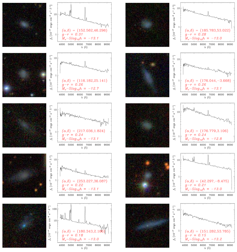
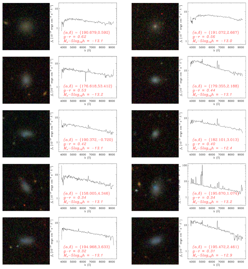
Figures 1a and 1b show the SDSS $gri$ images and $3^{\prime\prime}$ fiber spectra for the 20 lowest luminosity galaxies in our sample. The color images are prepared using the method of Lupton et al. (2004). They are sorted by color, reddest to bluest. These low luminosity galaxies tend to be blue, unconcentrated, have very little structure, and no noticeable dust lanes. These properties are consistent with previous studies of faint galaxies (e.g., Marzke & da Costa 1997; Bromley et al. 1998; Madgwick et al. 2002). They are mostly emission-line galaxies. Among these 20 galaxies, only the reddest two would be classified as dEs, according to their colors and spectra (one of these two is nucleated).

As noted in the introduction, the advantage of our catalog is its well-defined selection criteria. For comparison, the more local catalog of Karachentsev et al. (2004) (limited roughly at 7 $h^{-1}$ Mpc) includes a large number of objects less luminous than those we study here, most of them closer than 2.5 $h^{-1}$ Mpc. In addition, their catalog covers the entire sky, allowing them to examine very local structures, while ours is restricted to the SDSS area. Finally, because they include HI-discovered galaxies and due to their efforts at spectroscopic follow-up on low surface brightness objects, they include some galaxies of much lower surface brightness than we include here. However, a disadvantage of their catalog is that it appears to have been selected using very heterogeneous criteria, making certain statistical studies difficult.

3 Surface brightness completeness

Low luminosity galaxies tend to be low surface brightness. For that reason, it is important to understand the surface brightness incompleteness of our catalog. There are three aspects of this incompleteness. First, in Section 3.1, we determine the completeness of the most recent version of the SDSS photometric catalog by testing the software on simulated data. In Section 3.2, we test this completeness empirically. Second, in Section 3.3, we determine the completeness of the SDSS spectroscopic targeting with respect to the photometric catalog. Third, in Section 3.4, we determine the redshift completeness of the SDSS spectroscopy for targets which have been observed. Section 3.5, summarizes the effects of surface brightness on selection.

3.1 The photometric catalog

We have examined the surface brightness completeness of the SDSS photometric survey using a fake data pipeline (also described in Blanton et al. 2005).

For the current project we create 2500 fake galaxies (each with one image in each of the five SDSS bands) with exponential profiles, blue colors typical of low surface brightness galaxies, of varying axis ratios, and of varying half-light surface brightnesses and magnitudes, in the ranges $18<\mu_{50,r}<26$ and $14<m_{r}<17.5$. The faint limit here is close to but slightly brighter than the SDSS spectroscopic limit of 17.77; as this limit is almost 100 times brighter than the photometric detection limit, the 30% difference between 17.5 and 17.77 is not important to our results. We distribute the fake stamps onto a random set of locations on the sky covered by SDSS fields. For each observation of an object in an SDSS field in each band, we convert the fake stamps to SDSS raw data units, convolve with the estimated seeing from the SDSS photometric pipeline, and add Poisson noise using the estimates of the gain. We add the resulting image to the real SDSS raw data, including the tiny effects of nonlinearity in the response and the less tiny flat-field variation as a function of column on the chip. We run the SDSS photometric pipeline photo (version v5_4_25, essentially that used in the SDSS DR2 release) on the resulting set of images to extract and measure objects. This procedure thus includes the effects of seeing, noise, and sky subtraction.

Using the resulting photometric catalog, we create a fake version of the value-added catalog of Blanton et al. (2004), resolving multiple observations and imposing the selection criteria in exactly the same way as for the full catalog, including star-galaxy separation and all of the other SDSS Main sample criteria used for spectroscopic target selection (Strauss et al. 2002). These criteria include an explicit half-light surface brightness limit at $\mu_{50,r}=24.5$. These steps ensure that the fake photometric sample is selected in the same manner as the real one in the NYU-VAGC.

Finally, we compare the resulting catalog to the input catalog in order to evaluate our completeness to surface brightness selection effects. We require that the output object have a center within 5^′′ and a Petrosian magnitude within 0.5 mag of the input object (since usually such a large magnitude discrepancy indicates that a separate, nearby object has been targeted). We should note here that in the actual catalog we have reinstated some objects by hand. We have not done so in the fake catalog, meaning that we slightly underestimate our completeness.

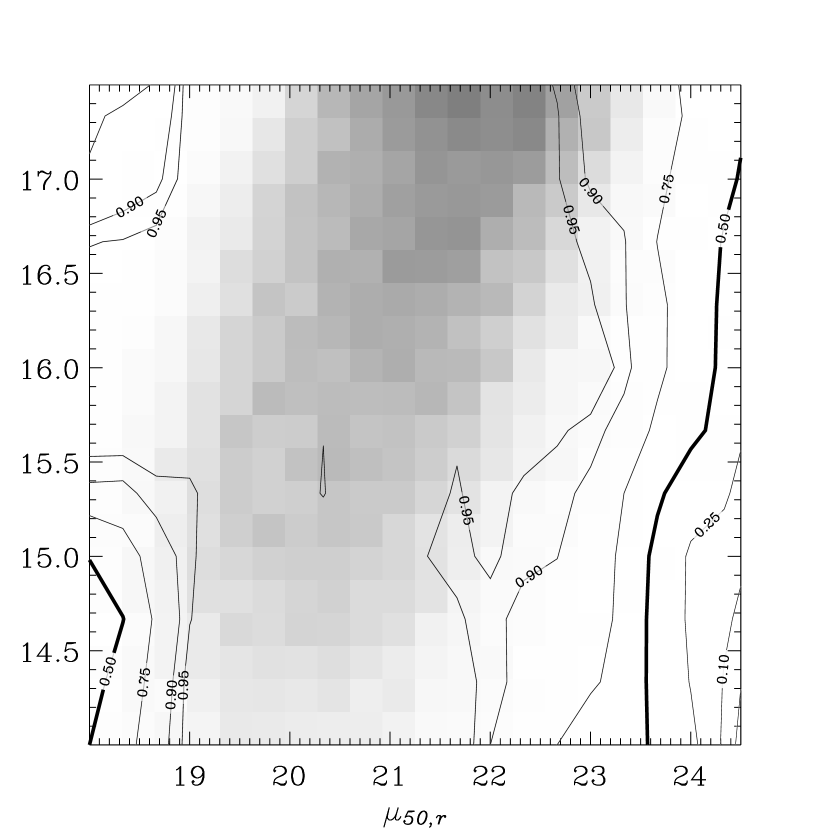
The contours in Figure 2 show the completeness thus calculated as a function of input half-light surface brightness and input total magnitude. The underlying greyscale image is the distribution of galaxies in the real galaxy catalog. Several features are prominent. First, in the lower left, small, bright objects have a low completeness. This occurs because of the lower limit on size of $\theta_{50}>2$ arcsec imposed in the Main sample selection criteria for objects with $m_{r}<15.5$ in order to eliminate double stars (Strauss et al. 2002). Second, in the upper left, there is incompleteness in faint, high surface brightness objects. This incompleteness results from the star-galaxy separator, which confuses such objects for stars in marginal seeing (such as in the SDSS fields we are testing here, for which the seeing is 1.5^′′ or so). We find that in better seeing conditions, this corner of the plot is nearly complete. Neither of these features are of particular interest here (though it is worth noting that there is a class of compact galaxies that this incompleteness affects, among them M32 and the UCDs of Deady et al. 2002). The greyscale shows that very few objects are observed in these regimes; in addition, since low luminosity objects tend to be lower surface brightness than average, these incompletenesses at high surface brightness are unimportant for the low luminosity galaxies.

However, on the right side it is clear that there is significant incompleteness at low surface brightness (more or less independent of size). A very small fraction of all SDSS galaxies are affected by this incompleteness, since the galaxy distribution declines long before it becomes important. However, low luminosity galaxies are disproportionately affected by the incompleteness, because they tend to be low surface brightness, and so for the purposes of this paper we must consider this effect.

The incompleteness at low surface brightness is due primarily to two effects. First, there is sometimes inappropriate shredding by the photometric deblender of low surface brightness galaxies, often related to the presence of nearby stars. This shredding tends to reduce the galaxy fluxes to well below the flux limits of the survey. Second, for many galaxies the flux is significantly reduced because the sky subtraction determination (a 100 by 100 arcsec median filter) subtracts a substantial fraction of the galaxy light (Strauss et al. 2002).

At low surface brightness the completeness is nearly independent of apparent magnitude in Figure 2. Therefore, we compress the information by averaging across apparent magnitude, weighting by the number of objects at each magnitude. This procedure yields the dot-dashed curve in Figure 3, the photometric catalog completeness $f_{\mathrm{ph}}(\mu_{50,r})$ as a function of half-light surface brightness. Table 1 gives the values used to make this figures.

We emphasize that this examination reveals the limits of the SDSS software, not the SDSS data. The photometric pipeline was not optimized for finding low-surface brightness objects, and there are many more detectable objects in the data. For example, essentially every object in our simulations (down to $\mu_{50,r}=26$) yields a large contiguous region of $5\sigma$ detected pixels; the non-detections of the catalog are due to deblending and mis-estimates of the sky. This accords with the results of Cross et al. (2004), who find for the deeper Millenium Galaxy Catalog that $\sim 90\%$ of their objects yielded SDSS detections even at $\mu_{B}\sim 26$. We further note that all the galaxies in the nearby catalog of Karachentsev et al. (2004) that fall within the SDSS area are of high signal-to-noise ratio in the raw data and flagged as pixels with signal, even if in the catalog they are deblended into many shreds or otherwise excluded from the spectroscopic survey, as many of these very nearby ($<10$ Mpc) galaxies are. These facts motivate an effort to recover even lower surface brightness objects from the data and to weed out the considerable background of data defects, such as internal reflections of bright stars. Such an effort has been begun by Kniazev et al. (2004).

3.2 Empirical test using Galactic extinction

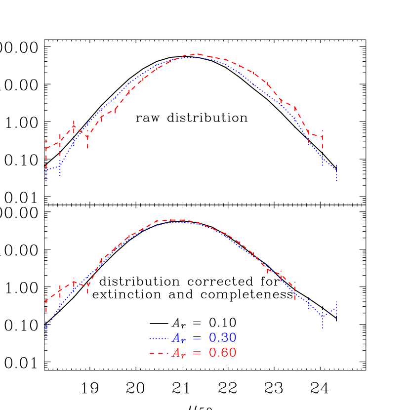
We can test the surface brightness completeness of the photometric catalog in a different manner, following Davies et al. (1993). The observed surface brightness distribution of galaxies is shifted faintward by Galactic extinction by an amount that depends on direction and is predicted by Schlegel et al. (1998). The top panel of Figure 4 shows this trend for all galaxies with an extinction-corrected Petrosian magnitude $m_{r}<18$. We use three bins of Galactic extinction centered on the values shown. Each curve is the surface density of galaxies as a function of Petrosian half-light surface brightness for the given Galactic extinction, in units that are the same for each bin of extinction.

The distribution of intrinsic surface brightness should not depend on the amount of intervening Galactic dust. So if we correct the surface brightness of each galaxy in the sample for the estimated dust extinction, and correct the surface density using the completeness estimate above (according to the observed surface brightness, of course), the curves should be independent of the extinction. Indeed, the bottom panel of Figure 4 shows these distributions, which lie on each other quite well.

These figures make clear two points. First, for the bulk of SDSS galaxies, surface brightness completeness issues are irrelevant. Second, we have reasonable estimates of our completeness at the lowest surface brightness end, which we will use below to attempt to judge what constraints we can make on the low luminosity slope of the luminosity function.

3.3 The tiling catalog

The above tests evaluate the completeness of the catalog of SDSS objects using the most recent version of the photometric pipeline. However, as we found above, the completeness has as much to do with the photometric software as it has to do with the data itself. Furthermore, the software has changed over the course of the survey. Of particular interest here, the deblender has improved substantially. Earlier versions tended to incorrectly shred large galaxies into multiple parts. When low surface brightness galaxies were shredded they often had their flux reduced enough that no part of them was targeted. Although, as found above, this problem persists in the later reductions, software improvements have greatly mitigated it. All of the spectroscopic targeting used here was performed on the v5_2 version of the photometric pipeline, or previous. Thus, we need to evaluate what fraction of the objects detected in the v5_4 results actually were targeted by the old version of the software.

To evaluate this completeness we ask what fraction of NYU-VAGC galaxies brighter than the spectroscopic flux limit in each region of sky (see Blanton et al. 2004) have matches in the “tiling catalog,” the list of targets actually selected for spectroscopy by the SDSS. We denote this fraction $f_{\mathrm{ti}}(\mu_{50,r})$.

There is a subtlety we must account for when considering the completeness of the survey, which is that the tiling completeness integrated over surface brightness is already included in the completeness as a function of position. The completeness as a function of position $f_{\mathrm{got}}(\alpha,\delta)$, given by the NYU-VAGC sample described in Blanton et al. (2004), is the fraction of galaxies brighter than the flux limit that are in the spectroscopic catalog, which is basically a subset of the tiling catalog. Thus, $f_{\mathrm{got}}(\alpha,\delta)$ effectively includes the tiling incompleteness integrated over all surface brightnesses. So in order to isolate just the surface brightness dependence of the tiling completeness, we scale our result according to the total tiling completeness:

$$\tilde{f}_{\mathrm{ti}}=\frac{f_{\mathrm{ti}}(\mu_{50,r})}{\int d\mu_{50,r}p(\mu_{50,r})f_{\mathrm{ti}}(\mu_{50,r})}$$ (2)

where $p(\mu_{50,r})$ is the probability density distribution of surface brightness. In practice, the denominator is around 0.97. Naturally, then, $\tilde{f}_{\mathrm{ti}}$ can exceed unity (slightly), which is compensated for on average by the fact that $f_{\mathrm{got}}(\alpha,\delta)$ is less than unity.

Figure 3 shows this completeness $\tilde{f}_{\mathrm{ti}}(\mu_{50,r})$ as a function of surface brightness as the dashed line, and Table 1 lists the values plotted.

3.4 The spectroscopic catalog

We determine the spectroscopic incompleteness as a function of surface brightness simply by looking at what fraction of Main sample targets whose spectra we attempted actually yielded reliable redshifts. Figure 3 shows this fraction $f_{\mathrm{sp}}(\mu_{50,r})$ as a function of surface brightness; the bottom panel shows the number of objects used in each bin.

3.5 The total surface brightness completeness function

In order to evaluate the total surface brightness completeness, we simply multiply together the three components above. Thus, the total completeness as a function of position and surface brightness may be expressed:

$$f(\mu_{50,r},\alpha,\delta)=\tilde{f}_{\mathrm{ti}}(\mu_{50,r}){f}_{\mathrm{sp}}(\mu_{50,r}){f}_{\mathrm{ph}}(\mu_{50,r})f_{\mathrm{got}}(\alpha,\delta)$$ (3)

Figure 3 shows this function (for a direction in which $f_{\mathrm{got}}(\alpha,\delta)=1$) as the solid line.

4 Luminosity function and properties of galaxies

4.1 Calculating the luminosity function

Because low luminosity galaxies tend to be low surface brightness, the surface brightness selection effects investigated in the previous section are likely to cause an underestimate of the luminosity function at low luminosities. Below, we will present three versions of the luminosity function:

1. the raw luminosity function for galaxies with surface brightnesses $\mu_{50,r}<24$, completely uncorrected for surface brightness selection effects;

2. the luminosity function for galaxies with surface brightnesses $\mu_{50,r}<24$, corrected for surface brightness incompleteness; and

3. an estimate of the total luminosity function using a model for the luminosity-surface brightness relationship.

The first two we calculate in all five bands; the last we only perform in the $r$ band.

We calculate the uncorrected luminosity function (1) for galaxies with $\mu_{50,r}<24$ using the step-wise maximum likelihood method (Efstathiou et al. 1988). An advantage of this method, compared to the $V_{\mathrm{max}}$ method (Schmidt 1968) or the method of Blanton et al. (2003c), is that those methods are susceptible to cosmic variance errors due to large-scale structure in the volume probed. That is, overdensities or voids can lead to artificial structure in the resulting luminosity function (or, in the case of the method of Blanton et al. 2003c, artificial number density evolution). Basically, the idea of Efstathiou et al. (1988) is to maximize the conditional likelihood of observing each galaxy to have its luminosity given its redshift. The exact method used here is described in more detail by Blanton et al. (2001).

To calculate the luminosity function (2) for galaxies with $\mu_{50,r}<24$, we use these same techniques but include only galaxies in that range of surface brightness and, in addition, weight each galaxy with $1/f(\mu_{50,r})$, the inverse of the completeness found in the previous section. In practice, this means taking the individual likelihood for each galaxy to the power $1/f(\mu_{50,r})$.

Finally, to estimate the numbers of galaxies missing below $\mu_{50,r}=24$ and thus the “total” luminosity function (3), we need to assume some model for the relationship between surface brightness and luminosity. To do so, we select galaxies with $n<2$ and $M_{r}<-18$. For such galaxies, the surface brightness limits are unimportant, as we will see below. We fit the following model to their conditional distribution in surface brightness as a function of magnitude:

$$P(\mu_{50,r}|M_{r})=\frac{1}{\sqrt{2\pi}\sigma_{\mu}}\exp\left[(\mu_{50,r}-{\bar{\mu}_{50,r}}(M_{r}))^{2}/2\sigma_{\mu}^{2}(M_{r})\right]$$ (4)

where

$${\bar{\mu}_{50,r}}(M_{r}) = \mu_{50,\ast}+\gamma(M_{r}+20.5)$$ (5)

$$\sigma_{\mu}(M_{r}) = \sigma_{\mu\ast}+\beta(M_{r}+20.5)$$ (6)

The distribution is thus a Gaussian in surface brightness at all absolute magnitudes, with a power law relationship between absolute magnitude and the mean (linearly expressed) surface brightness. We allow the width of the distribution to grow linearly as the absolute magnitude increases. Note that we do not specify the normalization at each absolute magnitude. In this definition, $\mu_{50,\ast}$ is the typical surface brightness of an exponential galaxy around $M_{\ast}\sim-20.5$. Our best fit is $\gamma=0.45$, $\mu_{50,\ast}=20.56$, $\beta=0.081$, and $\sigma_{\mu\ast}=0.58$.

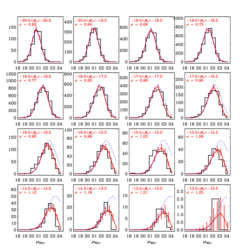
Figure 5 shows the surface brightness distribution in bins of absolute magnitude. The histogram is the observed distribution. The dotted line is the model of Equation 4. The solid line is the model multiplied by the photometric and spectroscopic completenesses from Table 1. The lines are normalized to minimize the residuals between the solid line and the solid histogram. The error bars on the solid lines assume Poisson statistics.

The model is good in the range over which we have fit ($M_{r}<-18$). As stated above, it is clear that in this regime galaxies lie safely away from the surface brightness limits of the survey. Less luminous than that ($M_{r}>-18$), for which the model represents an extrapolation, there are some deviations. In particular, the observed distribution appears to have a slightly larger tail on the high surface brightness end than the model assumes.

We use this model to estimate the possible magnitude of surface brightness selection effects as $c$, the ratio of two integrals: that of the solid line to that of the dotted line. That is, our estimate is the fraction of galaxies in our model which would be observable given our estimated completeness. Figure 6 shows the resulting “correction” factor one should therefore apply as a function of absolute magnitude.

By weighting by $c$, we obtain the “total” luminosity function (3). This estimate is obviously highly uncertain, since the model of Equation 4 does not necessarily represent the surface brightness distribution below our detection limits. However, it is our best guess at what could reasonably be missing.

4.2 The luminosity function and the luminosity density

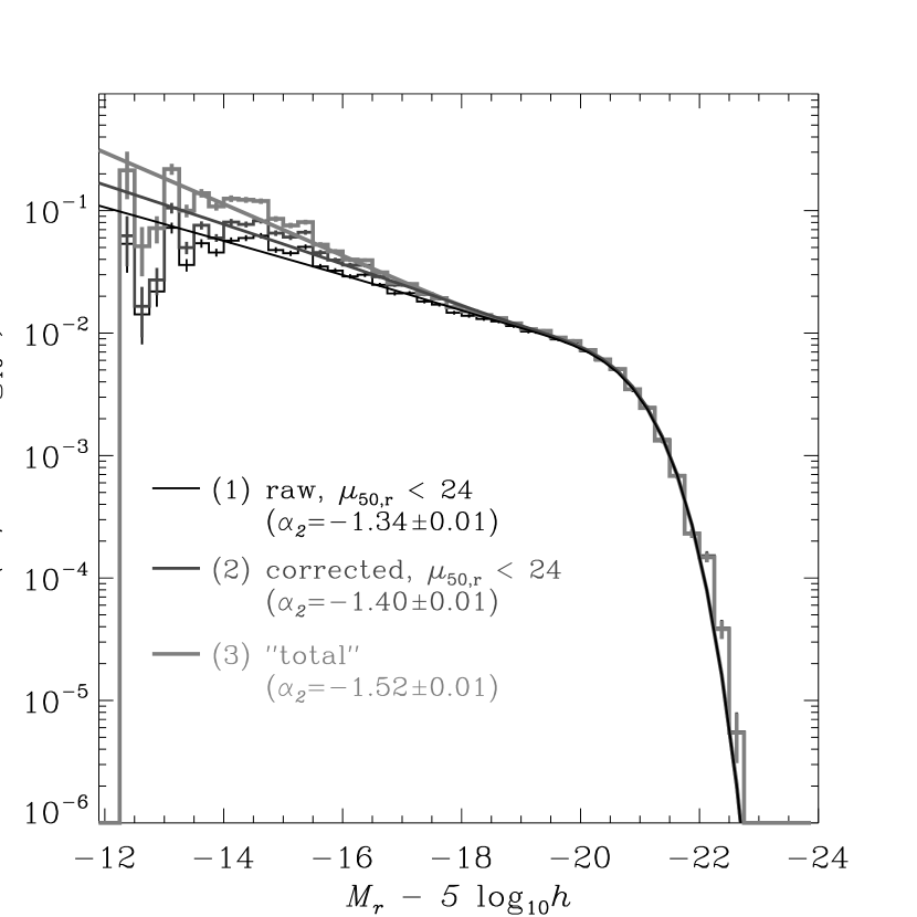
Figure 7 shows the luminosity function of our sample calculated using the step-wise maximum likelihood estimator. The black histogram shows (1), the luminosity function for galaxies with $\mu_{50,r}<24$ uncorrected for surface brightness incompleteness and represents a “minimum” abundance of galaxies. The dark grey represents (2), the luminosity function of galaxies with $\mu_{50,r}<24$ corrected for incompleteness. The light grey histogram represents (3), the “total” luminosity function using the method of Section 4.1 to “correct” for missing galaxies below the surface brightness limits. Note that this third estimate, while it represents a reasonable extrapolation of the abundance of galaxies at these luminosities, is not an actual measurement of it. We claim that an abundance of low luminosity galaxies similar to the light grey histogram cannot be ruled out from any current data. Table 2 gives the values used for the histograms in Figure 7.

The smooth lines in Figure 7 represent fits to the luminosity function using a double Schechter function:

$$\Phi(L)dL=\frac{dL}{L_{\ast}}\exp(-L/L_{\ast})\left[\phi_{\ast,1}\left(\frac{L}{L_{\ast}}\right)^{\alpha_{1}}+\phi_{\ast,2}\left(\frac{L}{L_{\ast}}\right)^{\alpha_{2}}\right]$$ (7)

Stated in terms of absolute magnitude $M=-2.5\log_{10}(L)+$ const this equation is:

$$\Phi(M)=0.4\ln 10dM\exp\left(-10^{-0.4(M-M_{\ast})}\right)\left[\phi_{\ast,1}10^{-0.4\left(M-M_{\ast}\right)(\alpha_{1}+1)}+\phi_{\ast,2}10^{-0.4\left(M-M_{\ast}\right)(\alpha_{2}+1)}\right]$$ (8)

This function is a much better fit than a single Schechter function, which fails to capture the upturn in the luminosity function at $M_{r}\sim-18$ or so. Although the luminosity function is nearly flat at luminosities higher than that (and less than $L_{\ast}$), even the uncorrected, “minimal” luminosity function turns up to a slope of about $\alpha_{2}\sim-1.3$ below that luminosity. As shown in the fit to the solid histogram, surface brightness selection effects may imply a much steeper slope, possibly steeper than $\alpha_{2}\sim-1.5$. The full set of parameters found in these fits are listed in Table 5 (listed in terms of $M_{\ast}$).

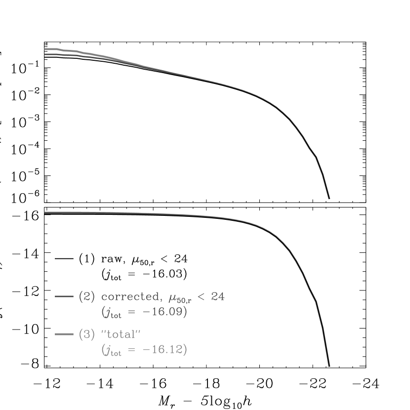
The top panel of Figure 8 shows the cumulative number density distribution of galaxies brighter than $M_{r}$ as a function of $M_{r}$, for all three versions of the luminosity function. The bottom panel of Figure 8 similarly shows the luminosity density, in units of absolute magnitudes per $h^{-1}$ Mpc³. The total luminosity density in these units is $-16.02$ for the uncorrected case (1), and $-16.12$ for the “total” case (3). Note that, even for the “total” case, most of the luminosity density ($>90\%$) is contained in galaxies with $M_{r}<-17$. That is, as noted by a number of authors in the past (McGaugh 1996; Sprayberry et al. 1997; Blanton et al. 2001; Cross et al. 2001; Blanton et al. 2003b) the contribution of low luminosity and low surface brightness galaxies to the overall optical luminosity density appears small.

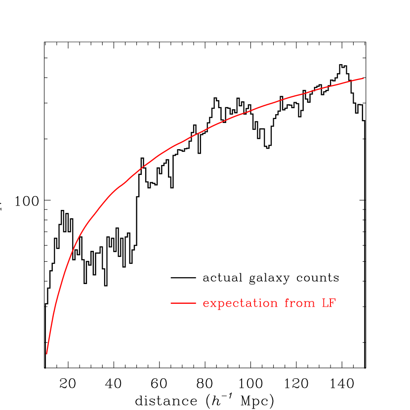
Figure 9 shows the distance distribution of galaxies based on our best-fit distances. The smooth line is the expected distribution given the raw luminosity function (1). Note there is change by a factor of $\sim 2$ in the mean density of galaxies in the local volume covered by this sample, which appears to be an underdensity in the nearby section of the volume covered by this sample. The fluctuation is within a volume of about 2 $\times$ $10^{4}$ $h^{-3}$ Mpc³, equivalent to about a $\sim 20$ $h^{-1}$ Mpc radius sphere. Given the results of Tegmark et al. (2004), whose constraints come from galaxy clustering over much larger volumes, we expect $\sigma_{20}\sim 0.5$. Thus, the structure we observe is consistent with what we know about clustering of galaxies on large scales using more distant samples (which is itself consistent with predictions based on cosmic microwave background and other observations).

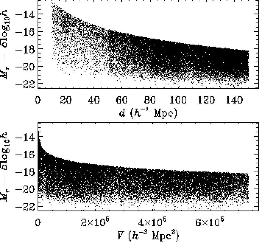
Figure 10 shows the joint distribution of redshift and absolute magnitude in the top panel, and of enclosed volume and absolute magnitude in the bottom panel. Note there is a decrease in the density of galaxies at small volumes, corresponding to the change in the overdensity of galaxies seen in Figure 9. For the most luminous galaxies, there is something of a decline towards small volumes, probably indicative of a bias against large objects due to the SDSS selection process. This bias comes from the fact that large galaxies are often deblended incorrectly by the SDSS photometric pipeline, because they often have complex structure and because they often run into the edges of fields. For future versions of this catalog, we will concentrate on a more complete sample at the bright end to resolve these problems; however, the focus of this paper is on the low luminosity galaxies, so we ignore this potential problem for the moment.

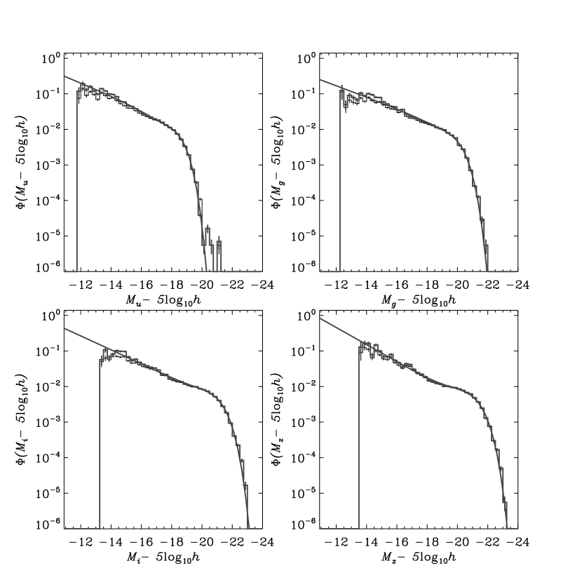
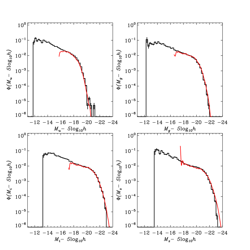
In addition, we calculate the luminosity function in the $ugiz$ bands using the step-wise maximum likelihood method and compare our result to those of Blanton et al. (2003c). In order to calculate each luminosity function, we restrict our sample to galaxies for which $m_{u}<18.4$, $m_{g}<17.7$, $m_{i}<17.5$, or $m_{z}<16.9$, depending on which band we are interested in. At each magnitude limit we are highly complete in the given band (Blanton et al. 2001). We follow the same procedure as we did in calculating the $r$-band luminosity function. Figure 11 shows the results of this procedure for the raw luminosity function for galaxies with $\mu_{50,r}<24$ (1) as the black histograms. The version for galaxies with $\mu_{50,r}<24$ corrected for incompleteness (2) appears as the grey histograms. The smooth lines are the double Schechter function fits we describe above fit to each of the corrected luminosity functions. Tables 3 and 4 tabulate the results for the uncorrected and the corrected case, respectively. Table 5 lists the double Schechter function parameters for each luminosity function. Note that Baldry et al. (2005) suspect large sky subtraction errors to add considerable scatter to the $u$-band magnitudes of spectroscopic galaxies; our luminosity function here does not use the empirical corrections they recommend.

4.3 Comparison to the $V_{\mathrm{max}}$ method

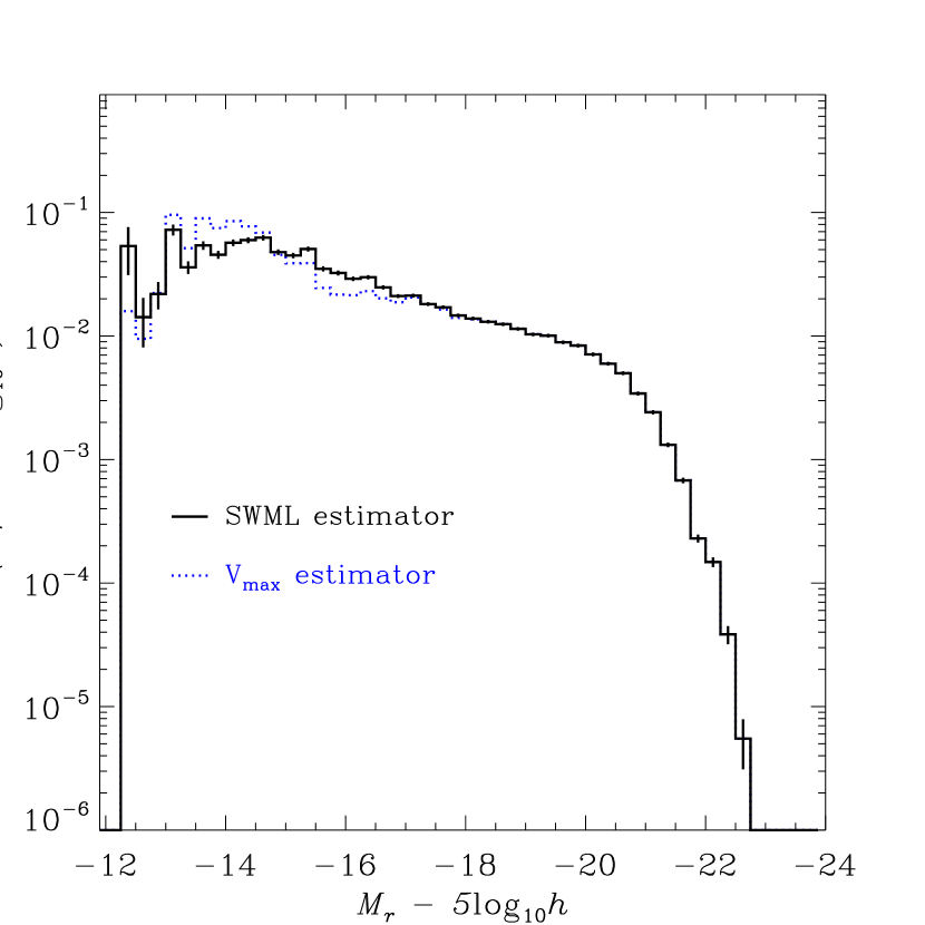
Figure 12 shows a comparison of our original (uncorrected) luminosity function using the step-wise maximum likelihood method and that obtained using the $1/V_{\mathrm{max}}$ method. The $1/V_{\mathrm{max}}$ method is more susceptible to the effects of large-scale structure (dotted histogram). These two estimates are in good agreement at the bright end (where they probe a large amount of volume), though some of the features in the $V_{\mathrm{max}}$ result appear to be due to large-scale structure. In particular, the overdensity closer than 20 $h^{-1}$ Mpc and the underdensity in the range 30–50 $h^{-1}$ Mpc in Figure 9 appear to result in a corresponding overestimate of the luminosity function at about $M_{r}-5\log_{10}h\sim-14$ and an underestimate at about $M_{r}-5\log_{10}h\sim-16$. We show these results to give a sense of the possible errors in the distributions of galaxy properties weighted by $1/V_{\mathrm{max}}$ shown in Section 4.6. These errors are significant but not overwhelming. The $V_{\mathrm{max}}$ results are listed in Table 2.

4.4 Comparison to the literature

There exist previous SDSS results using the full sample of galaxies out to a redshift $z=0.22$ (Blanton et al. 2003c). Those results are quoted in the ${}^{0.1}\!{ugriz}$ bands, which are the $ugriz$ bands shifted blueward by a factor 1.1 (Blanton et al. 2003), and are evolution correction to an effective redshift of $z=0.1$. We can calculate the photometric transformations from ${}^{0.1}\!{ugriz}$ to $ugriz$ based on the SED models fit by kcorrect v3_2, for galaxies of median intrinsic ${}^{0.1}\!{(g-r)}$ color. This procedure yields the relationships:

$$u = {}^{0.1}\!{u}-0.38$$ (9)

$$g = {}^{0.1}\!{g}-0.41$$ (10)

$$r = {}^{0.1}\!{r}-0.22$$ (11)

$$i = {}^{0.1}\!{i}-0.19$$ (12)

$$z = {}^{0.1}\!{z}-0.11$$ (13)

We correct for evolution using the luminosity evolution model of Blanton et al. (2003c):

$$M(z) = M(z=0.1)-(z-0.1)Q$$ (14)

$${\bar{n}}(z) = {\bar{n}}(z=0.1)10^{0.4(z-0.1)P}$$ (15)

where $Q=4.22,2.04,1.62,1.61,0.76$ and $P=0.20,0.32,0.18,0.58,2.28$ in the $ugriz$ bands.

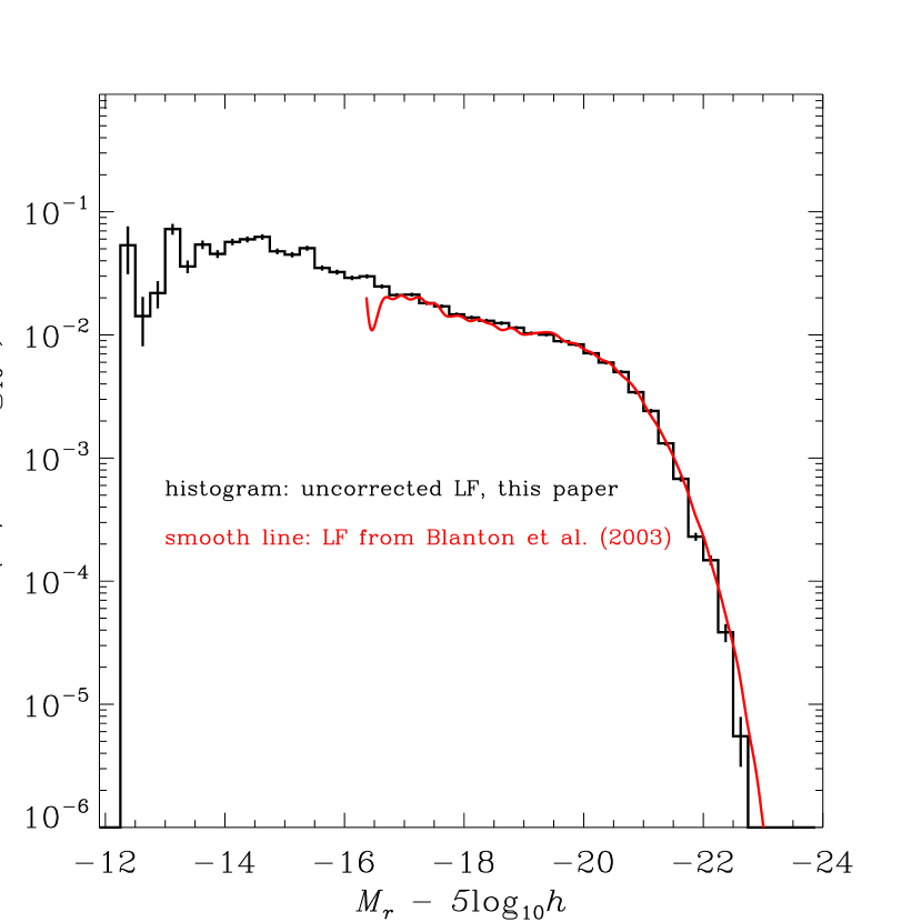
Figure 14 shows the raw luminosity function (1) in the $r$-band for our sample compared to the results of Blanton et al. (2003c), shown as the solid line. Figure 11 shows the comparison for the $ugiz$ bands. The agreement between the determinations is good in the range measured by Blanton et al. (2003c).

It is worth noting that both the current results and those of Blanton et al. (2003c) differ markedly from those of Blanton et al. (2001), whose results are incorrect because they ignored the effects of evolution on the normalization and slope of the luminosity function. These effects are fully described in Blanton et al. (2003c), which describes exactly why the Blanton et al. (2001) is in error. Essentially, the volume-weighted normalization allowed the tiny number density of high luminosity objects to carry large statistical weight. Since the luminosity function is so steep at high luminosity, a small evolution in absolute magnitude resulted in a large change in number density at fixed absolute magnitude. For this paper, we have been able to ignore the effects of evolution because we are considering such a small redshift range. For example, the $Q=1.62$ evolution in the $r$-band found by Blanton et al. (2003c) leads to a magnitude difference across this sample of only about $0.08$. In addition, this sample is volume-limited for $M_{r}<-18.5$, so the steepness of the luminosity function at the luminous end is not as important as it was in the more distant sample of Blanton et al. (2001).

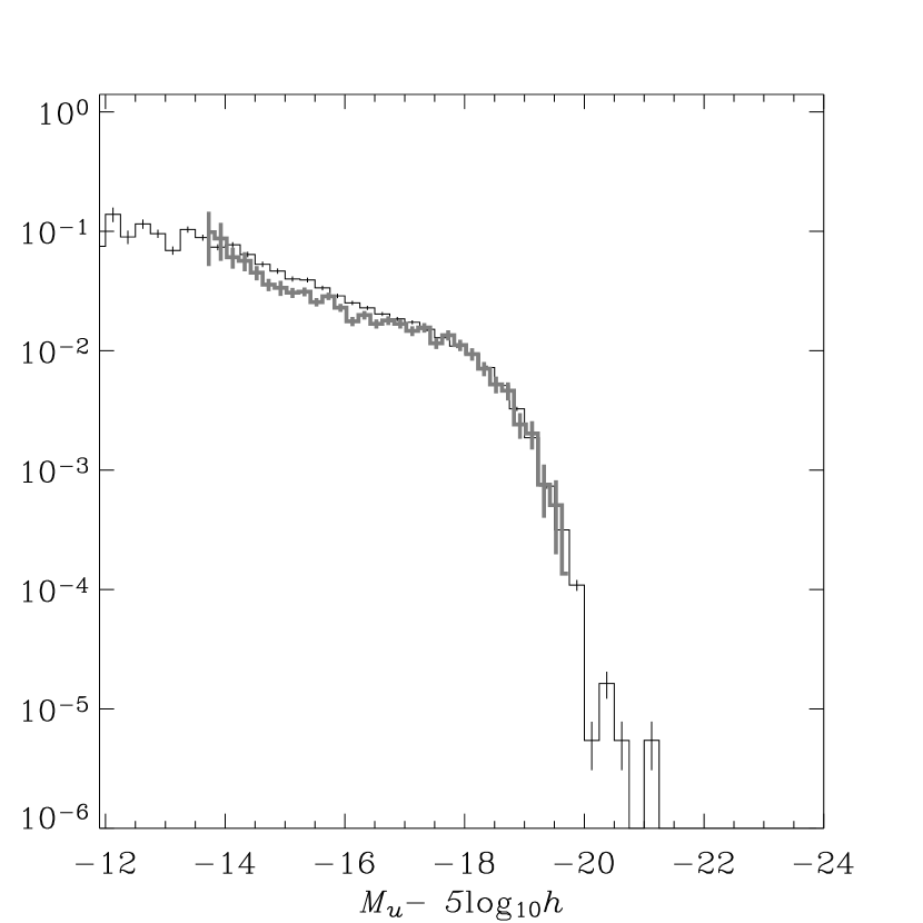
Baldry et al. (2005) have measured the luminosity function in the $u$ band using a deeper (but more heterogeneously selected) SDSS sample and accounting for systematic errors in $u$-band sky subtraction which we ignore here. Figure 13 compares our result with their results in the redshift range $0.02<z<0.04$. The results are similar, though at the low luminosity end there is about a 20% discrepancy in the density found in our sample and in their sample. The Baldry et al. (2005) sample is restricted to the 275 square degrees covered by the SDSS Southern Survey, which raises the possibility that the difference is simply cosmic variance.

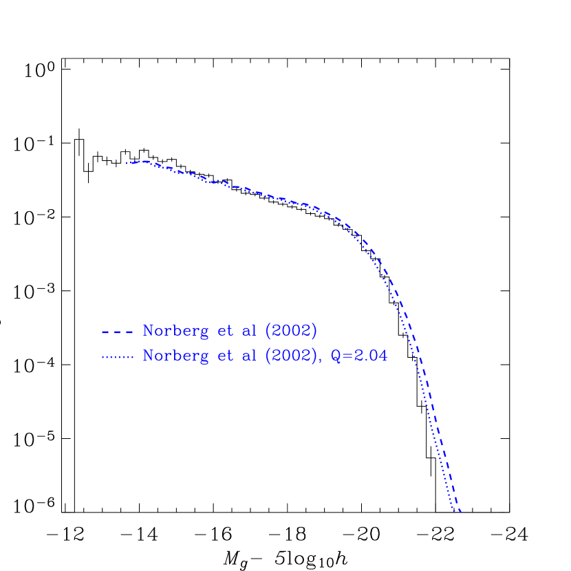
In addition, Figure 16 compares the $g$ band luminosity function to that of Norberg et al. (2002). We convert the result of Norberg et al. (2002) in the $b_{j}$ band to $g$ using the relationship $g=b_{j}-0.25$. The dashed line in Figure 16 shows the result of converting their luminosity function this way. There are significant differences between our $g$-band luminosity function and that of Norberg et al. (2002). However, the slope at low luminosities is very similar. Furthermore, we note that the luminosity evolution assumed by Norberg et al. (2002) is close to $Q=1.0$, much less than the empirical luminosity evolution in the $g$-band $Q=2.04$ found by Blanton et al. (2003c) and less than the theoretical estimate $Q=1.60$ of Bell et al. (2003). An extremely simplistic way of accounting for this difference at high luminosities is to simply shift their absolute magnitudes by $\Delta Qz_{m}$, where $z_{m}=0.16$ is their median redshift for galaxies with $M_{g}<-19.7$ and $\Delta Q=1.04$ is the difference between the effective evolution assumptions of Norberg et al. (2002) and the empirical estimates of Blanton et al. (2004). This shift brings the results more closely in line with each other at the luminous end, though fainter than that there are still $20$–$30\%$ differences in the luminosity functions.

A real comparison may require a more careful understanding of the different treatment of $K$-corrections and evolution in Norberg et al. (2002) and Blanton et al. (2003c). $K$-corrections at $z=0.25$, the limit of the sample of Norberg et al. (2002), are significant; they can be up to 0.9 mag in the $g$ band. For the SDSS bands, Blanton et al. (2003) have shown that the $K$-corrections recover fairly consistent intrinsic colors of galaxies as a function of redshift, but this has not been shown with respect to the $b_{j}$ band, and inconsistencies at the 10–20% level have not been ruled out. The effects of evolution are smaller, but much more poorly known; theoretical estimates of the evolution do not agree with one another, and the empirical measurement of Blanton et al. (2003c) is by no means definitive.

The SDSS and the 2dFGRS are the most complete and well-studied redshift surveys of the local universe, and aside from the roughly 0.15 mag disagreement in $M_{\ast}$ they are in fairly good agreement on the overall shape of the luminosity function. There are no important discrepancies in the low luminosity slope.

4.5 Comparison between environments

We can compare these field luminosity functions to those determined in the SDSS from studies of clusters and voids. We leave for a future paper the task of comparing the luminosity function in different regions of our own sample, and here will concentrate on comparison to the literature.

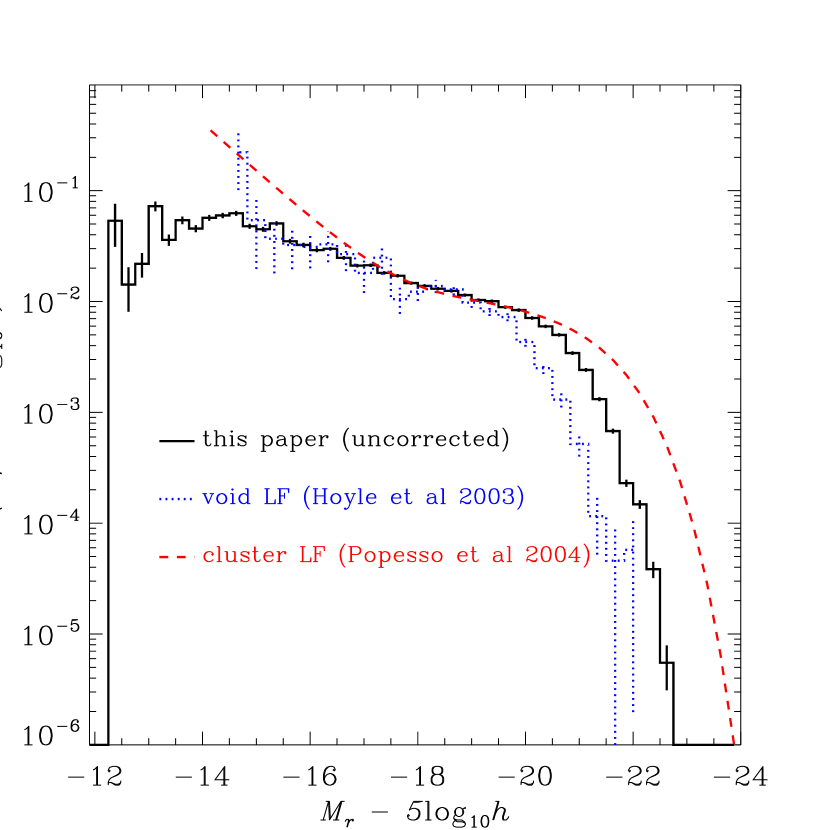
Popesso et al. (2004) have used statistical background subtraction on the photometric catalog to measure the optical luminosity function around X-ray clusters without recourse to determining redshifts. Similar methods have been used on other cluster samples by a number of authors, such as Schechter (1976); Gaidos (1997); Valotto et al. (1997); Garilli et al. (1999); Paolillo et al. (2001); Andreon & Cuillandre (2002); Goto et al. (2002). We will not attempt here a comparison among all of those efforts. Figure 17 shows the best-fit double Schechter function result of Popesso et al. (2004) compared to our raw luminosity function (1). The exponential cut-off is clearly much brighter in clusters. In addition, the low luminosity slope is much steeper below $M_{r}\sim-17$. Note that the results of Popesso et al. (2004) should be free of the background subtraction biases in cluster luminosity functions described by Valotto et al. (2001), since the clusters are selected from X-ray observations rather than the galaxy counts themselves.

Both of the luminosity functions in Figure 17 are susceptible to surface brightness selection effects. However, it is possible that these effects are less important in the Popesso et al. (2004) results, since they do not apply the target selection limit of $\mu_{50,r}<24.5$ that affects the spectroscopic results.

Figure 17 also shows the luminosity function of SDSS void galaxies found by Hoyle et al. (2005). Their luminosity function is affected by exactly the same surface brightness limits as this paper is. For these galaxies, there is a significantly less luminous exponential cut-off, but the low luminosity slope is remarkably similar to that of the field galaxy population.

4.6 Luminosity function as a function of galaxy properties

The luminosity function is known to be a function of galaxy type — among the many papers on this subject are those of Binggeli et al. (1988); Roberts & Haynes (1994); Marzke et al. (1994); Marzke & da Costa (1997); Bromley et al. (1998); Madgwick et al. (2002); Blanton et al. (2003b). In this section, we explore this dependence using the sample at hand.

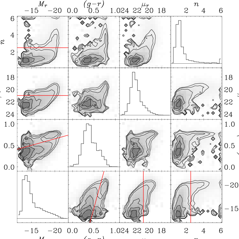
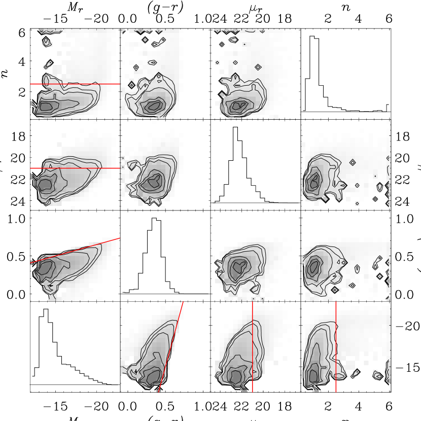
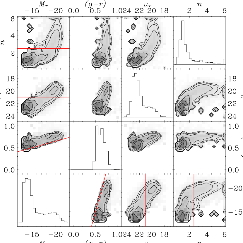
Figure 18 shows the number density distribution of galaxy properties (determined, in this case, using the 1/$V_{\mathrm{max}}$ estimator for convenience). We have not corrected these plots for surface brightness incompleteness in any way. The diagonal plots show the number density distribution of absolute magnitude $M_{r}$, color $g-r$, $r$-band half-light surface brightness $\mu_{50,r}$, and Sérsic index $n$. The off-diagonal plots show the bivariate number distribution between each pair of properties as contours and a greyscale. Many of the qualitative features in this plot are extensions of the relationships found in Blanton et al. (2003b) for more luminous galaxies ($M_{r}<-17$). Low luminosity galaxies are bluer, lower surface brightness, and more exponential than high luminosity galaxies. Note that at low luminosity (say $M_{r}>-16$ or so) the surface brightness selection at around $\mu_{50,r}\sim 24$ clearly becomes important.

In the left column, one can see the luminosity function as a function of color, surface brightness and Sérsic index. The principal trend which is evident is the large density of red, low luminosity galaxies. We have seen above that these red, low luminosity galaxies are preferentially in dense regions.

In order to investigate the properties of these red galaxies somewhat further, we split the sample along color using the following, luminosity-dependent cut:

$$(g-r)_{c}=0.65-0.03(M_{r}+20)$$ (16)

This dividing line, shown as the tilted line in the appropriate panel of Figure 18, is approximately at the bottom edge of the red sequence. Figure 19 shows the galaxies defined as blue by this cut. Even at high luminosity, these tend to be low surface brightness and not particularly concentrated. Figure 20 shows the galaxies defined as red. The strong dependence of Sérsic index and surface brightness on luminosity is evident for the red galaxies. The lowest luminosity ones are as unconcentrated and low surface brightness as the correspondingly luminous blue galaxies, and generally are featureless and similar morphologically to dE galaxies. In addition, one can easily see that they have comparable space densities to more luminous red galaxies.

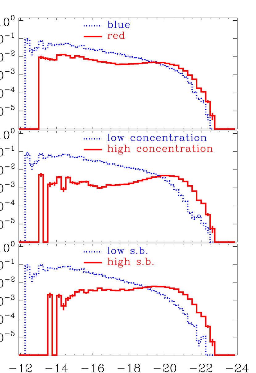
In order to better see the luminosity functions of galaxies of various types, Figure 21 shows the raw luminosity function (1) for galaxies split into two categories, in three different ways: by color, as in Equation 16; by Sérsic index, dividing the population at $n=2.5$; and by surface brightness, dividing the population at $\mu_{50,r}=21$. We show the locations of these cuts as lines in Figure 18. As in the previous plots, here we see that a large fraction of low luminosity galaxies are blue, low concentration, and low surface brightness.

5 Summary

We have presented a sample and basic properties of a set of low redshift ($z<0.05$) galaxies in the SDSS. Most interestingly, this sample is the only sample of galaxies extending down to $M_{r}\sim-12.5$ which is unbiased with respect to environment.

From our measurements of the properties of these galaxies and of their luminosity function, we conclude:

1. The slope of the luminosity function at low luminosities ($M_{r}-5\log_{10}h>-17$), here denoted $\alpha_{2}$, is at least as steep as $-1.3$, though it is almost certainly steeper, and perhaps as steep as $-1.5$.

2. Galaxies at these low luminosities are low in surface brightness, close to exponential, and predominantly blue.

3. Our estimate of the luminosity function is strongly affected by surface brightness selection effects at low luminosities. We have taken some care in estimating the completeness in this regime.

4. Incompleteness at low luminosities hardly affects our estimated total luminosity density because even with our completeness corrections the low lumosity galaxies do not contribute significantly.

5. There is not a large discrepancy between the SDSS and 2dFGRS determinations of the luminosity function.

6. Comparing void, field, and cluster luminosity functions in the SDSS yields the conclusions that the exponential cut-off at high luminosities is a strong function of environment and that $\alpha_{2}$ is not a function of environment at low density, but may become significantly steeper at high density.

There are a number of important improvements we can make to the measurements described here:

1. With later data releases of the SDSS, we can explore more of the local volume, of which we do not yet have a fair sample. In particular, we will be observing regions surrounding and including the Virgo cluster. This increased volume will allow a better measurement of the environmental dependence of the properties of low luminosity galaxies.

2. Deeper SDSS spectroscopy to $m_{r}<19.5$, targeted at galaxies thought to be at $z<0.1$ according to photometric redshifts, may result in improved statistics on the abundance of low luminosity galaxies (Lin et al, in preparation).

3. Improved analysis of the SDSS imaging will allow us to detect low surface brightness galaxies. First, in the Southern Equatorial stripe of the SDSS, we have many epochs of imaging, which will allow us to detect galaxies by their diffuse light. Second, Willman et al. (2002) and Zucker et al. (2004) continue to search for very nearby galaxies detected in resolved stars. These samples will allow us to evaluate the effects of surface brightness completeness on the low luminosity slope empirically.

4. In order to improve the sample at the luminous end, we will supplement the SDSS redshifts with known large, bright galaxies from the astronomical literature, in a statistically meaningful way.

These last two items will allow us to probe the regime below 10 $h^{-1}$ Mpc, which we have excluded here because of the current incompleteness of the catalog in that regime. In addition to examining even lower luminosity galaxies, we will be able to perform a more direct comparison with the work of Karachentsev et al. (2004) at these distances.

With the data in hand, we will be studying further the environmental dependence of galaxy properties, analyzing the images to better understand the morphology of galaxies over a large range of luminosities, and seeking to perform follow-up observations to better understand the mass-to-light ratios, star-formation histories, and dust content of extremely low luminosity galaxies in the field.

Figure 1a: SDSS $gri$ images and 3^′′ fiber spectra for the 20 lowest luminosity galaxies in our sample (all of which $M_{r}+5\log_{10}h>-13.2$). Each image is 57^′′ on a side. The spectrum in each case is associated with the center of the image. We have sorted them by $g-r$ color, starting with the reddest.

Figure 1b: Continuation of Figure 1a.

Figure 2: Contours indicate the completeness of the SDSS photometric sample used here as a function of half-light surface brightness and magnitude, as determined from the fake data pipeline described in the text. The underlying greyscale image is the distribution of real galaxies in the low-redshift catalog.

Figure 3: Solid line is the completeness as a function of surface brightness (for a direction in which $f_{\mathrm{got}}(\alpha,\delta)=1$. The contribution due to spectroscopic incompleteness is the dotted line. The contribution due to the tiling incompleteness is the dashed line. The contribution due to photometric incompleteness (estimated from simulations) is the dot-dashed line.

Figure 4: Top panel shows the distribution of galaxies as a function of surface brightness (determined from the Sérsic fit) uncorrected for Galactic extinction, in three bins of extinction, as labeled. Bottom panel shows the same distribution corrected for Galactic extinction and surface brightness incompleteness. There is no evidence for additional incompleteness.

Figure 5: Each panel shows as a histogram the distribution of surface brightness $\mu_{50,r}$ for a bin of absolute magnitude $M_{r}$. The dotted line is the model of Equation 4 as fit to galaxies more luminous than $M_{r}=-18$. The solid line is the model multiplied by the surface brightness completeness.

Figure 6: Estimate of possible correction factor due to surface brightness incompleteness in the SDSS, as a function of absolute magnitude. Based on fit of Equation 4 to luminosity surface brightness relationship at high luminosity ($M_{r}<-18$).

Figure 7: The luminosity function in the $r$-band calculated using the step-wise maximum likelihood method, with bins of width 0.25 mag. The black histogram is the minimal luminosity function (1) for galaxies with $\mu_{50,r}<24$, described in Section 4.1, with no correction for surface brightness selection effects. The dark grey histogram is the luminosity function for galaxies with $\mu_{50,r}<24$ corrected for surface brightness incompleteness. The light grey histogram is an attempt to estimate how many galaxies there might be using a simple model for the luminosity surface brightness relationship. The values used in this plot are given in Table 7. The smooth curves are double Schechter function fits to each result, whose parameters are given in Table 5. The bottom panel is the number of galaxies contributing to each bin. All magnitudes here and elsewhere in the paper are $K$-corrected to rest-frame bandpasses and have no evolution correction applied.

Figure 8: Top panel: Total number density in galaxies more luminous than $M_{r}$, as a function of $M_{r}$, for all three luminosity functions of Figure 7. The black line is the raw luminosity function for galaxies with $\mu_{50,r}<24$ (1); the dark grey line is the corrected luminosity function for galaxies with $\mu_{50,r}<24$ (2), and the dashed line is our estimate of the “total” luminosity function (3), all as described in Section 4.1. Bottom panel: Same as top panel for total luminosity density. In all cases, most of the luminosity density ($\sim 90\%$) is contained in galaxies with $M_{r}<-17$.

Figure 9: Histogram of distances to galaxies in the sample, in 1 $h^{-1}$ Mpc thick shells. The smooth line represents the expected number in each bin based on the best fit raw luminosity function (version 1) described in Section 4.1.

Figure 10: Top panel shows the joint distribution of distance and absolute magnitude. Bottom panel shows the joint distribution of enclosed volume and absolute magnitude. The distribution of galaxies in this plot shows a fairly constant distribution further than $z\sim 0.015$ ($V\sim 2\times 10^{4}$). However, there is noticeable large-scale structure interior to that, as well as some likely incompleteness at the luminous end of the distribution.

Figure 11: The histograms in each panel are similar to that in the top panel of Figure 7, for the $ugiz$ bands, as labeled. The black histograms correspond to the raw luminosity function for galaxies with $\mu_{50,r}<24$, version (1) in Section 4.1. The grey histograms correspond to the luminosity function for galaxies with with $\mu_{50,r}<24$ corrected for surface brightness incompleteness, version (2) in Section 4.1. For the $ugiz$ bands, we have not created a luminosity function corresponding to version (3) in that section. The smooth lines correspond to the double Schechter function fits the surface brightness corrected luminosity function version (2), whose parameters we list in Table 5.

Figure 12: Similar to Figure 7, but showing only the uncorrected results for the step-wise maximum likelihood method (solid histogram) and the $V_{\mathrm{max}}$ method (dotted histogram). There is complete agreement at high luminosity, but disagreement at low luminosity, probably due to large-scale structure affecting the $V_{\mathrm{max}}$ estimate.

Figure 13: Similar to Figure 7, but showing only the uncorrected results in the $u$-band (thin black) compared to the results of Baldry et al. (2005) (thick grey histogram). The results are similar, though there is a 20% discrepancy at the low luminosity end.

Figure 14: Similar to Figure 7, but showing only the uncorrected results for the step-wise maximum likelihood method (histogram) compared to the results of Blanton et al. (2003c). The two methods agree well.

Figure 15: The histogram in each panel is identical to those in Figure 11. The smooth solid line is the corresponding result from Blanton et al. (2003c), evolution and $K$-corrected to $z=0$.

Figure 16: Similar to Figure 7, but showing the uncorrected results for the step-wise maximum likelihood method in the $g$-band (histogram) compared to the results of of Norberg et al. (2002) (dashed line). There is a fairly large discrepancy, much of which can be explained by the weaker luminosity evolution assumed by Norberg et al. (2002). The dotted line shows how the high luminosity end would be shifted if we assume the stronger evolution measured by Blanton et al. (2003c).

Figure 17: Similar to Figure 7, but showing the uncorrected results for the step-wise maximum likelihood method in the $r$-band (histogram) compared to the results for void galaxies (Hoyle et al. 2005) and for cluster galaxies (Popesso et al. 2004).

Figure 18: Number density distribution of galaxy properties. All images have a square-root stretch applied to increase the dynamic range of the plot. Contours indicate the regions containing 10%, 30%, 50%, 70%, 90%, 95%, and 97% of the total number of galaxies in this sample. The upper and low triangles are identical mirror images. The histograms along the diagonal show the density distribution of galaxies in each dimension. We have weighted each galaxy with $1/V_{\mathrm{max}}$ to get the number density distribution of galaxies. The lines indicate the cuts used in Figures 19–21. These densities have not been corrected for surface brightness incompleteness in any way.

Figure 19: Similar to Figure 18, but for the blue galaxies (those bluer than the $(g-r)$ cut shown). Generally these objects are low luminosity, exponential, and low surface brightness.

Figure 20: Similar to Figure 18, but for the red galaxies (those redder than the $(g-r)$ cut shown). Note the very strong relationships among absolute magnitude, surface brightness, and Sérsic index for these red galaxies.

Figure 21: Raw luminosity function (1) found using the step-wise maximum likelihood method for galaxies split in three different ways: using the $(g-r)$ cut of Equation 16, at $n=2.5$, and at $\mu_{50,r}=21$ (the cuts shown as the lines in Figure 18).

Table 1: Surface brightness completeness

$\mu_{50,r}$	$N$	$f_{\mathrm{ph}}(\mu_{50})$	$\tilde{f}_{\mathrm{ti}}(\mu_{50})$	$f_{\mathrm{sp}}(\mu_{50})$	$f(\mu_{50})$
18.16	32	0.78	0.82	1.00	0.64
18.49	144	0.86	0.93	1.00	0.80
18.81	344	0.95	0.98	1.00	0.93
19.14	809	0.98	1.01	1.00	0.99
19.46	1351	0.99	1.01	1.00	0.99
19.79	1747	0.97	1.01	1.00	0.98
20.11	2082	0.98	1.01	1.00	0.98
20.44	2480	0.98	1.01	1.00	0.98
20.76	2557	0.98	1.01	1.00	0.99
21.09	2672	0.97	1.00	1.00	0.97
21.41	2554	0.96	1.00	1.00	0.96
21.74	2334	0.96	0.99	1.00	0.94
22.06	1853	0.97	0.97	1.00	0.94
22.39	1469	0.94	0.95	1.00	0.88
22.71	940	0.86	0.89	0.99	0.76
23.04	490	0.84	0.87	0.96	0.71
23.36	165	0.76	0.72	0.91	0.50
23.69	47	0.63	0.68	0.78	0.33
24.01	8	0.44	0.38	0.56	0.09
24.34	5	0.33	0.00	0.00	0.00

Note. — As described in Section 3.5, the completeness as a function of surface brightness in any given direction $(\alpha,\delta)$ is the final column of this table multiplied by the window function $f_{\mathrm{got}}(\alpha,\delta)$ from Blanton et al. (2004). Note that $\tilde{f}_{\mathrm{ti}}(\mu_{50})>1$ in some cases, because it has had the overall tiling completeness divided out, as described in Section 3.3.

Table 2: $r$-band luminosity function

$M_{r}-5\log_{10}h$	$\Phi(M_{r}-5\log_{10}h)$	$\Phi(M_{r}-5\log_{10}h)$	$\Phi(M_{r}-5\log_{10}h)$	$\Phi(M_{r}-5\log_{10}h)$
	(raw, $\mu_{50,r}<24$)	(corrected, $\mu_{50,r}<24$)	(“total”)	(uncorrected, $V_{\mathrm{max}}$ method)
$-12.375$	$(5.36\pm 2.24)\times 10^{-2}$	$(6.25\pm 2.73)\times 10^{-2}$	$(21.35\pm 8.94)\times 10^{-2}$	$(1.59\pm 1.59)\times 10^{-2}$
$-12.625$	$(1.42\pm 0.61)\times 10^{-2}$	$(1.65\pm 0.73)\times 10^{-2}$	$(5.12\pm 2.21)\times 10^{-2}$	$(9.49\pm 0.95)\times 10^{-3}$
$-12.875$	$(2.19\pm 0.54)\times 10^{-2}$	$(2.72\pm 0.68)\times 10^{-2}$	$(7.19\pm 1.79)\times 10^{-2}$	$(2.23\pm 1.29)\times 10^{-2}$
$-13.125$	$(7.25\pm 0.73)\times 10^{-2}$	$(10.52\pm 1.03)\times 10^{-2}$	$(21.87\pm 2.22)\times 10^{-2}$	$(9.57\pm 2.27)\times 10^{-2}$
$-13.375$	$(3.60\pm 0.42)\times 10^{-2}$	$(4.99\pm 0.57)\times 10^{-2}$	$(10.00\pm 1.17)\times 10^{-2}$	$(5.14\pm 1.38)\times 10^{-2}$
$-13.625$	$(5.41\pm 0.42)\times 10^{-2}$	$(7.59\pm 0.58)\times 10^{-2}$	$(13.89\pm 1.09)\times 10^{-2}$	$(8.97\pm 1.57)\times 10^{-2}$
$-13.875$	$(4.56\pm 0.33)\times 10^{-2}$	$(5.99\pm 0.44)\times 10^{-2}$	$(10.82\pm 0.79)\times 10^{-2}$	$(7.48\pm 1.20)\times 10^{-2}$
$-14.125$	$(5.69\pm 0.34)\times 10^{-2}$	$(8.07\pm 0.48)\times 10^{-2}$	$(12.55\pm 0.76)\times 10^{-2}$	$(8.52\pm 1.09)\times 10^{-2}$
$-14.375$	$(5.98\pm 0.33)\times 10^{-2}$	$(7.73\pm 0.42)\times 10^{-2}$	$(12.26\pm 0.67)\times 10^{-2}$	$(7.72\pm 0.87)\times 10^{-2}$
$-14.625$	$(6.25\pm 0.32)\times 10^{-2}$	$(8.26\pm 0.41)\times 10^{-2}$	$(11.97\pm 0.61)\times 10^{-2}$	$(6.87\pm 0.69)\times 10^{-2}$
$-14.875$	$(4.78\pm 0.25)\times 10^{-2}$	$(6.56\pm 0.34)\times 10^{-2}$	$(8.57\pm 0.45)\times 10^{-2}$	$(4.53\pm 0.47)\times 10^{-2}$
$-15.125$	$(4.49\pm 0.22)\times 10^{-2}$	$(6.07\pm 0.30)\times 10^{-2}$	$(7.57\pm 0.38)\times 10^{-2}$	$(3.88\pm 0.37)\times 10^{-2}$
$-15.375$	$(5.06\pm 0.23)\times 10^{-2}$	$(6.66\pm 0.30)\times 10^{-2}$	$(8.06\pm 0.36)\times 10^{-2}$	$(3.89\pm 0.31)\times 10^{-2}$
$-15.625$	$(3.50\pm 0.17)\times 10^{-2}$	$(4.55\pm 0.21)\times 10^{-2}$	$(5.28\pm 0.25)\times 10^{-2}$	$(2.45\pm 0.21)\times 10^{-2}$
$-15.875$	$(3.24\pm 0.14)\times 10^{-2}$	$(3.95\pm 0.18)\times 10^{-2}$	$(4.65\pm 0.21)\times 10^{-2}$	$(2.16\pm 0.17)\times 10^{-2}$
$-16.125$	$(2.91\pm 0.12)\times 10^{-2}$	$(3.60\pm 0.15)\times 10^{-2}$	$(3.98\pm 0.17)\times 10^{-2}$	$(2.14\pm 0.14)\times 10^{-2}$
$-16.375$	$(2.99\pm 0.12)\times 10^{-2}$	$(3.58\pm 0.14)\times 10^{-2}$	$(3.93\pm 0.15)\times 10^{-2}$	$(2.31\pm 0.12)\times 10^{-2}$
$-16.625$	$(2.48\pm 0.09)\times 10^{-2}$	$(2.88\pm 0.11)\times 10^{-2}$	$(3.13\pm 0.12)\times 10^{-2}$	$(2.02\pm 0.10)\times 10^{-2}$
$-16.875$	$(2.11\pm 0.08)\times 10^{-2}$	$(2.47\pm 0.09)\times 10^{-2}$	$(2.58\pm 0.09)\times 10^{-2}$	$(1.88\pm 0.08)\times 10^{-2}$
$-17.125$	$(2.12\pm 0.07)\times 10^{-2}$	$(2.46\pm 0.09)\times 10^{-2}$	$(2.52\pm 0.09)\times 10^{-2}$	$(2.05\pm 0.07)\times 10^{-2}$
$-17.375$	$(1.81\pm 0.06)\times 10^{-2}$	$(2.07\pm 0.07)\times 10^{-2}$	$(2.09\pm 0.07)\times 10^{-2}$	$(1.81\pm 0.06)\times 10^{-2}$
$-17.625$	$(1.71\pm 0.06)\times 10^{-2}$	$(1.91\pm 0.06)\times 10^{-2}$	$(1.93\pm 0.07)\times 10^{-2}$	$(1.64\pm 0.05)\times 10^{-2}$
$-17.875$	$(1.47\pm 0.05)\times 10^{-2}$	$(1.63\pm 0.05)\times 10^{-2}$	$(1.63\pm 0.06)\times 10^{-2}$	$(1.40\pm 0.04)\times 10^{-2}$
$-18.125$	$(1.38\pm 0.05)\times 10^{-2}$	$(1.51\pm 0.05)\times 10^{-2}$	$(1.51\pm 0.05)\times 10^{-2}$	$(1.37\pm 0.03)\times 10^{-2}$
$-18.375$	$(1.30\pm 0.04)\times 10^{-2}$	$(1.40\pm 0.04)\times 10^{-2}$	$(1.40\pm 0.05)\times 10^{-2}$	$(1.31\pm 0.03)\times 10^{-2}$
$-18.625$	$(1.25\pm 0.04)\times 10^{-2}$	$(1.32\pm 0.04)\times 10^{-2}$	$(1.33\pm 0.04)\times 10^{-2}$	$(1.25\pm 0.03)\times 10^{-2}$
$-18.875$	$(1.14\pm 0.04)\times 10^{-2}$	$(1.20\pm 0.04)\times 10^{-2}$	$(1.20\pm 0.04)\times 10^{-2}$	$(1.14\pm 0.02)\times 10^{-2}$
$-19.125$	$(1.03\pm 0.04)\times 10^{-2}$	$(1.07\pm 0.03)\times 10^{-2}$	$(1.08\pm 0.04)\times 10^{-2}$	$(1.03\pm 0.02)\times 10^{-2}$
$-19.375$	$(1.01\pm 0.03)\times 10^{-2}$	$(1.04\pm 0.03)\times 10^{-2}$	$(1.05\pm 0.04)\times 10^{-2}$	$(1.01\pm 0.02)\times 10^{-2}$
$-19.625$	$(8.89\pm 0.30)\times 10^{-3}$	$(9.18\pm 0.29)\times 10^{-3}$	$(9.19\pm 0.31)\times 10^{-3}$	$(8.91\pm 0.22)\times 10^{-3}$
$-19.875$	$(8.37\pm 0.29)\times 10^{-3}$	$(8.65\pm 0.28)\times 10^{-3}$	$(8.61\pm 0.29)\times 10^{-3}$	$(8.39\pm 0.21)\times 10^{-3}$
$-20.125$	$(7.10\pm 0.25)\times 10^{-3}$	$(7.27\pm 0.23)\times 10^{-3}$	$(7.28\pm 0.25)\times 10^{-3}$	$(7.12\pm 0.20)\times 10^{-3}$
$-20.375$	$(5.96\pm 0.21)\times 10^{-3}$	$(6.14\pm 0.20)\times 10^{-3}$	$(6.09\pm 0.21)\times 10^{-3}$	$(5.98\pm 0.18)\times 10^{-3}$
$-20.625$	$(5.00\pm 0.18)\times 10^{-3}$	$(5.13\pm 0.17)\times 10^{-3}$	$(5.09\pm 0.18)\times 10^{-3}$	$(5.01\pm 0.17)\times 10^{-3}$
$-20.875$	$(3.43\pm 0.13)\times 10^{-3}$	$(3.51\pm 0.12)\times 10^{-3}$	$(3.48\pm 0.13)\times 10^{-3}$	$(3.43\pm 0.14)\times 10^{-3}$
$-21.125$	$(2.42\pm 0.09)\times 10^{-3}$	$(2.48\pm 0.09)\times 10^{-3}$	$(2.44\pm 0.09)\times 10^{-3}$	$(2.42\pm 0.11)\times 10^{-3}$
$-21.375$	$(1.32\pm 0.06)\times 10^{-3}$	$(1.35\pm 0.06)\times 10^{-3}$	$(1.33\pm 0.06)\times 10^{-3}$	$(1.32\pm 0.08)\times 10^{-3}$
$-21.625$	$(6.78\pm 0.34)\times 10^{-4}$	$(6.89\pm 0.34)\times 10^{-4}$	$(6.81\pm 0.35)\times 10^{-4}$	$(6.78\pm 0.61)\times 10^{-4}$
$-21.875$	$(2.30\pm 0.17)\times 10^{-4}$	$(2.33\pm 0.17)\times 10^{-4}$	$(2.30\pm 0.17)\times 10^{-4}$	$(2.30\pm 0.35)\times 10^{-4}$
$-22.125$	$(1.48\pm 0.13)\times 10^{-4}$	$(1.52\pm 0.14)\times 10^{-4}$	$(1.48\pm 0.13)\times 10^{-4}$	$(1.48\pm 0.28)\times 10^{-4}$
$-22.375$	$(3.84\pm 0.64)\times 10^{-5}$	$(3.90\pm 0.66)\times 10^{-5}$	$(3.82\pm 0.64)\times 10^{-5}$	$(3.84\pm 1.45)\times 10^{-5}$
$-22.625$	$(5.50\pm 2.40)\times 10^{-6}$	$(5.54\pm 2.44)\times 10^{-6}$	$(5.45\pm 2.37)\times 10^{-6}$	$(5.51\pm 5.51)\times 10^{-6}$

Note. — Column 2 is the raw luminosity function for galaxies with $\mu_{50,r}<24$, corresponding to luminosity function (1) in Section 4.1. Column 3 is the luminosity function of galaxies with $\mu_{50,r}<24$ corrected for surface brightness incompleteness, corresponding to luminosity function (2) in Section 4.1. Column 4 is the “total” luminosity function using the method described in Section 4.1 to “correct” for the estimated missing fraction, corresponding to luminosity function (3) in that section. Column 5 is deprecated and is only given so the reader can evaluate the large-scale structure effects in the $1/V_{\mathrm{max}}$ weighted plots of Figures 18–20.

Table 3: $ugiz$-band luminosity functions

$M-5\log_{10}h$	$\Phi(M_{u}-5\log_{10}h)$	$\Phi(M_{g}-5\log_{10}h)$	$\Phi(M_{i}-5\log_{10}h)$	$\Phi(M_{z}-5\log_{10}h)$
$-11.875$	$(7.49\pm 2.23)\times 10^{-2}$	—	—	—
$-12.125$	$(1.39\pm 0.19)\times 10^{-1}$	—	—	—
$-12.375$	$(8.97\pm 1.15)\times 10^{-2}$	$(1.12\pm 0.45)\times 10^{-1}$	—	—
$-12.625$	$(1.15\pm 0.10)\times 10^{-1}$	$(4.13\pm 1.25)\times 10^{-2}$	—	—
$-12.875$	$(9.55\pm 0.76)\times 10^{-2}$	$(6.61\pm 1.09)\times 10^{-2}$	—	—
$-13.125$	$(6.91\pm 0.54)\times 10^{-2}$	$(5.78\pm 0.78)\times 10^{-2}$	—	—
$-13.375$	$(1.04\pm 0.06)\times 10^{-1}$	$(5.34\pm 0.62)\times 10^{-2}$	$(5.03\pm 1.50)\times 10^{-2}$	—
$-13.625$	$(8.85\pm 0.51)\times 10^{-2}$	$(7.63\pm 0.64)\times 10^{-2}$	$(6.31\pm 1.08)\times 10^{-2}$	$(9.07\pm 3.72)\times 10^{-2}$
$-13.875$	$(7.37\pm 0.42)\times 10^{-2}$	$(6.10\pm 0.49)\times 10^{-2}$	$(5.69\pm 0.76)\times 10^{-2}$	$(1.24\pm 0.21)\times 10^{-1}$
$-14.125$	$(7.70\pm 0.41)\times 10^{-2}$	$(7.99\pm 0.55)\times 10^{-2}$	$(7.17\pm 0.68)\times 10^{-2}$	$(1.10\pm 0.14)\times 10^{-1}$
$-14.375$	$(6.39\pm 0.34)\times 10^{-2}$	$(6.39\pm 0.44)\times 10^{-2}$	$(7.12\pm 0.55)\times 10^{-2}$	$(6.40\pm 0.85)\times 10^{-2}$
$-14.625$	$(5.29\pm 0.28)\times 10^{-2}$	$(5.62\pm 0.39)\times 10^{-2}$	$(6.74\pm 0.45)\times 10^{-2}$	$(1.01\pm 0.09)\times 10^{-1}$
$-14.875$	$(4.65\pm 0.24)\times 10^{-2}$	$(6.01\pm 0.39)\times 10^{-2}$	$(6.92\pm 0.41)\times 10^{-2}$	$(7.78\pm 0.65)\times 10^{-2}$
$-15.125$	$(3.99\pm 0.20)\times 10^{-2}$	$(4.84\pm 0.32)\times 10^{-2}$	$(5.29\pm 0.32)\times 10^{-2}$	$(5.98\pm 0.49)\times 10^{-2}$
$-15.375$	$(3.91\pm 0.18)\times 10^{-2}$	$(4.08\pm 0.26)\times 10^{-2}$	$(4.57\pm 0.28)\times 10^{-2}$	$(5.72\pm 0.44)\times 10^{-2}$
$-15.625$	$(3.35\pm 0.15)\times 10^{-2}$	$(3.77\pm 0.24)\times 10^{-2}$	$(4.64\pm 0.26)\times 10^{-2}$	$(6.85\pm 0.47)\times 10^{-2}$
$-15.875$	$(2.88\pm 0.12)\times 10^{-2}$	$(3.64\pm 0.22)\times 10^{-2}$	$(4.10\pm 0.22)\times 10^{-2}$	$(4.70\pm 0.34)\times 10^{-2}$
$-16.125$	$(2.51\pm 0.10)\times 10^{-2}$	$(2.98\pm 0.18)\times 10^{-2}$	$(3.66\pm 0.19)\times 10^{-2}$	$(3.98\pm 0.29)\times 10^{-2}$
$-16.375$	$(2.28\pm 0.09)\times 10^{-2}$	$(3.16\pm 0.18)\times 10^{-2}$	$(3.38\pm 0.17)\times 10^{-2}$	$(3.28\pm 0.24)\times 10^{-2}$
$-16.625$	$(2.03\pm 0.08)\times 10^{-2}$	$(2.34\pm 0.13)\times 10^{-2}$	$(3.11\pm 0.15)\times 10^{-2}$	$(3.92\pm 0.25)\times 10^{-2}$
$-16.875$	$(1.85\pm 0.07)\times 10^{-2}$	$(2.09\pm 0.11)\times 10^{-2}$	$(2.94\pm 0.13)\times 10^{-2}$	$(3.69\pm 0.23)\times 10^{-2}$
$-17.125$	$(1.73\pm 0.07)\times 10^{-2}$	$(2.02\pm 0.11)\times 10^{-2}$	$(2.66\pm 0.11)\times 10^{-2}$	$(2.81\pm 0.17)\times 10^{-2}$
$-17.375$	$(1.51\pm 0.06)\times 10^{-2}$	$(1.80\pm 0.10)\times 10^{-2}$	$(2.07\pm 0.08)\times 10^{-2}$	$(2.30\pm 0.14)\times 10^{-2}$
$-17.625$	$(1.28\pm 0.05)\times 10^{-2}$	$(1.59\pm 0.08)\times 10^{-2}$	$(2.01\pm 0.08)\times 10^{-2}$	$(2.05\pm 0.12)\times 10^{-2}$
$-17.875$	$(1.09\pm 0.04)\times 10^{-2}$	$(1.49\pm 0.08)\times 10^{-2}$	$(1.59\pm 0.06)\times 10^{-2}$	$(1.78\pm 0.10)\times 10^{-2}$
$-18.125$	$(9.37\pm 0.36)\times 10^{-3}$	$(1.37\pm 0.07)\times 10^{-2}$	$(1.46\pm 0.05)\times 10^{-2}$	$(1.44\pm 0.08)\times 10^{-2}$
$-18.375$	$(7.23\pm 0.28)\times 10^{-3}$	$(1.27\pm 0.07)\times 10^{-2}$	$(1.35\pm 0.05)\times 10^{-2}$	$(1.32\pm 0.07)\times 10^{-2}$
$-18.625$	$(5.11\pm 0.20)\times 10^{-3}$	$(1.11\pm 0.06)\times 10^{-2}$	$(1.30\pm 0.05)\times 10^{-2}$	$(1.21\pm 0.07)\times 10^{-2}$
$-18.875$	$(3.26\pm 0.13)\times 10^{-3}$	$(1.02\pm 0.05)\times 10^{-2}$	$(1.15\pm 0.04)\times 10^{-2}$	$(1.14\pm 0.06)\times 10^{-2}$
$-19.125$	$(1.87\pm 0.08)\times 10^{-3}$	$(9.47\pm 0.50)\times 10^{-3}$	$(1.05\pm 0.04)\times 10^{-2}$	$(9.97\pm 0.54)\times 10^{-3}$
$-19.375$	$(7.35\pm 0.38)\times 10^{-4}$	$(7.76\pm 0.41)\times 10^{-3}$	$(9.77\pm 0.33)\times 10^{-3}$	$(10.00\pm 0.54)\times 10^{-3}$
$-19.625$	$(3.16\pm 0.21)\times 10^{-4}$	$(6.78\pm 0.36)\times 10^{-3}$	$(9.63\pm 0.33)\times 10^{-3}$	$(9.35\pm 0.50)\times 10^{-3}$
$-19.875$	$(1.09\pm 0.11)\times 10^{-4}$	$(5.64\pm 0.30)\times 10^{-3}$	$(8.57\pm 0.29)\times 10^{-3}$	$(9.05\pm 0.49)\times 10^{-3}$
$-20.125$	$(5.44\pm 2.37)\times 10^{-6}$	$(3.49\pm 0.19)\times 10^{-3}$	$(8.02\pm 0.28)\times 10^{-3}$	$(8.31\pm 0.45)\times 10^{-3}$
$-20.375$	$(1.63\pm 0.41)\times 10^{-5}$	$(2.72\pm 0.15)\times 10^{-3}$	$(7.21\pm 0.25)\times 10^{-3}$	$(7.64\pm 0.41)\times 10^{-3}$
$-20.625$	$(5.44\pm 2.37)\times 10^{-6}$	$(1.54\pm 0.09)\times 10^{-3}$	$(6.15\pm 0.22)\times 10^{-3}$	$(6.64\pm 0.36)\times 10^{-3}$
$-20.875$	—	$(6.86\pm 0.44)\times 10^{-4}$	$(5.10\pm 0.18)\times 10^{-3}$	$(6.04\pm 0.33)\times 10^{-3}$
$-21.125$	$(5.45\pm 2.37)\times 10^{-6}$	$(2.51\pm 0.21)\times 10^{-4}$	$(3.97\pm 0.14)\times 10^{-3}$	$(4.73\pm 0.26)\times 10^{-3}$
$-21.375$	—	$(1.25\pm 0.13)\times 10^{-4}$	$(2.72\pm 0.10)\times 10^{-3}$	$(3.64\pm 0.20)\times 10^{-3}$
$-21.625$	—	$(2.73\pm 0.55)\times 10^{-5}$	$(1.79\pm 0.07)\times 10^{-3}$	$(2.41\pm 0.14)\times 10^{-3}$
$-21.875$	—	$(5.47\pm 2.39)\times 10^{-6}$	$(9.19\pm 0.43)\times 10^{-4}$	$(1.27\pm 0.08)\times 10^{-3}$
$-22.125$	—	—	$(4.00\pm 0.24)\times 10^{-4}$	$(7.50\pm 0.48)\times 10^{-4}$
$-22.375$	—	—	$(2.19\pm 0.17)\times 10^{-4}$	$(2.96\pm 0.23)\times 10^{-4}$
$-22.625$	—	—	$(8.24\pm 0.96)\times 10^{-5}$	$(1.65\pm 0.16)\times 10^{-4}$
$-22.875$	—	—	$(1.65\pm 0.42)\times 10^{-5}$	$(4.95\pm 0.76)\times 10^{-5}$
$-23.125$	—	—	—	$(5.52\pm 2.41)\times 10^{-6}$

Note. — We have not corrected these luminosity functions for surface brightness incompleteness at all; they correspond to luminosity function (1) in Section 4.1.

Table 4: $ugiz$-band luminosity functions, surface brightness completeness corrected

$M-5\log_{10}h$	$\Phi(M_{u}-5\log_{10}h)$	$\Phi(M_{g}-5\log_{10}h)$	$\Phi(M_{i}-5\log_{10}h)$	$\Phi(M_{z}-5\log_{10}h)$
$-11.875$	$(1.19\pm 0.34)\times 10^{-1}$	—	—	—
$-12.125$	$(1.93\pm 0.26)\times 10^{-1}$	—	—	—
$-12.375$	$(1.30\pm 0.16)\times 10^{-1}$	$(1.25\pm 0.54)\times 10^{-1}$	—	—
$-12.625$	$(1.61\pm 0.14)\times 10^{-1}$	$(4.95\pm 1.52)\times 10^{-2}$	—	—
$-12.875$	$(1.20\pm 0.10)\times 10^{-1}$	$(9.14\pm 1.47)\times 10^{-2}$	—	—
$-13.125$	$(9.83\pm 0.77)\times 10^{-2}$	$(7.86\pm 1.04)\times 10^{-2}$	—	—
$-13.375$	$(1.40\pm 0.08)\times 10^{-1}$	$(6.80\pm 0.79)\times 10^{-2}$	$(5.68\pm 1.74)\times 10^{-2}$	—
$-13.625$	$(1.21\pm 0.07)\times 10^{-1}$	$(1.06\pm 0.09)\times 10^{-1}$	$(1.08\pm 0.17)\times 10^{-1}$	$(1.29\pm 0.51)\times 10^{-1}$
$-13.875$	$(9.93\pm 0.59)\times 10^{-2}$	$(8.80\pm 0.70)\times 10^{-2}$	$(6.66\pm 0.94)\times 10^{-2}$	$(1.67\pm 0.28)\times 10^{-1}$
$-14.125$	$(9.59\pm 0.52)\times 10^{-2}$	$(1.02\pm 0.07)\times 10^{-1}$	$(8.14\pm 0.81)\times 10^{-2}$	$(1.64\pm 0.20)\times 10^{-1}$
$-14.375$	$(8.33\pm 0.46)\times 10^{-2}$	$(9.40\pm 0.65)\times 10^{-2}$	$(1.02\pm 0.08)\times 10^{-1}$	$(7.72\pm 1.04)\times 10^{-2}$
$-14.625$	$(6.04\pm 0.33)\times 10^{-2}$	$(7.98\pm 0.55)\times 10^{-2}$	$(9.80\pm 0.64)\times 10^{-2}$	$(1.49\pm 0.13)\times 10^{-1}$
$-14.875$	$(5.91\pm 0.31)\times 10^{-2}$	$(7.86\pm 0.50)\times 10^{-2}$	$(9.74\pm 0.57)\times 10^{-2}$	$(9.96\pm 0.85)\times 10^{-2}$
$-15.125$	$(4.60\pm 0.24)\times 10^{-2}$	$(5.96\pm 0.38)\times 10^{-2}$	$(6.89\pm 0.42)\times 10^{-2}$	$(6.94\pm 0.59)\times 10^{-2}$
$-15.375$	$(4.44\pm 0.21)\times 10^{-2}$	$(5.17\pm 0.33)\times 10^{-2}$	$(5.35\pm 0.33)\times 10^{-2}$	$(6.83\pm 0.55)\times 10^{-2}$
$-15.625$	$(3.84\pm 0.17)\times 10^{-2}$	$(4.45\pm 0.27)\times 10^{-2}$	$(5.91\pm 0.33)\times 10^{-2}$	$(8.08\pm 0.57)\times 10^{-2}$
$-15.875$	$(3.22\pm 0.14)\times 10^{-2}$	$(4.31\pm 0.25)\times 10^{-2}$	$(4.84\pm 0.27)\times 10^{-2}$	$(5.49\pm 0.41)\times 10^{-2}$
$-16.125$	$(2.76\pm 0.12)\times 10^{-2}$	$(3.43\pm 0.19)\times 10^{-2}$	$(4.22\pm 0.22)\times 10^{-2}$	$(4.69\pm 0.35)\times 10^{-2}$
$-16.375$	$(2.51\pm 0.10)\times 10^{-2}$	$(3.64\pm 0.20)\times 10^{-2}$	$(3.85\pm 0.19)\times 10^{-2}$	$(3.59\pm 0.26)\times 10^{-2}$
$-16.625$	$(2.20\pm 0.09)\times 10^{-2}$	$(2.68\pm 0.14)\times 10^{-2}$	$(3.51\pm 0.17)\times 10^{-2}$	$(4.41\pm 0.30)\times 10^{-2}$
$-16.875$	$(1.98\pm 0.08)\times 10^{-2}$	$(2.34\pm 0.12)\times 10^{-2}$	$(3.33\pm 0.15)\times 10^{-2}$	$(4.15\pm 0.27)\times 10^{-2}$
$-17.125$	$(1.83\pm 0.07)\times 10^{-2}$	$(2.23\pm 0.11)\times 10^{-2}$	$(2.95\pm 0.12)\times 10^{-2}$	$(3.07\pm 0.20)\times 10^{-2}$
$-17.375$	$(1.59\pm 0.06)\times 10^{-2}$	$(1.98\pm 0.10)\times 10^{-2}$	$(2.27\pm 0.09)\times 10^{-2}$	$(2.49\pm 0.15)\times 10^{-2}$
$-17.625$	$(1.34\pm 0.05)\times 10^{-2}$	$(1.73\pm 0.09)\times 10^{-2}$	$(2.20\pm 0.08)\times 10^{-2}$	$(2.24\pm 0.14)\times 10^{-2}$
$-17.875$	$(1.13\pm 0.04)\times 10^{-2}$	$(1.59\pm 0.08)\times 10^{-2}$	$(1.74\pm 0.07)\times 10^{-2}$	$(1.90\pm 0.11)\times 10^{-2}$
$-18.125$	$(9.68\pm 0.37)\times 10^{-3}$	$(1.45\pm 0.07)\times 10^{-2}$	$(1.57\pm 0.06)\times 10^{-2}$	$(1.54\pm 0.09)\times 10^{-2}$
$-18.375$	$(7.44\pm 0.29)\times 10^{-3}$	$(1.33\pm 0.06)\times 10^{-2}$	$(1.45\pm 0.05)\times 10^{-2}$	$(1.41\pm 0.08)\times 10^{-2}$
$-18.625$	$(5.25\pm 0.21)\times 10^{-3}$	$(1.16\pm 0.05)\times 10^{-2}$	$(1.38\pm 0.05)\times 10^{-2}$	$(1.27\pm 0.07)\times 10^{-2}$
$-18.875$	$(3.34\pm 0.14)\times 10^{-3}$	$(1.06\pm 0.05)\times 10^{-2}$	$(1.21\pm 0.04)\times 10^{-2}$	$(1.19\pm 0.07)\times 10^{-2}$
$-19.125$	$(1.91\pm 0.08)\times 10^{-3}$	$(9.79\pm 0.47)\times 10^{-3}$	$(1.10\pm 0.04)\times 10^{-2}$	$(1.04\pm 0.06)\times 10^{-2}$
$-19.375$	$(7.52\pm 0.40)\times 10^{-4}$	$(8.04\pm 0.38)\times 10^{-3}$	$(1.01\pm 0.03)\times 10^{-2}$	$(1.04\pm 0.06)\times 10^{-2}$
$-19.625$	$(3.26\pm 0.22)\times 10^{-4}$	$(6.90\pm 0.33)\times 10^{-3}$	$(9.96\pm 0.34)\times 10^{-3}$	$(9.66\pm 0.53)\times 10^{-3}$
$-19.875$	$(3.84\pm 0.45)\times 10^{-5}$	$(5.79\pm 0.28)\times 10^{-3}$	$(8.83\pm 0.30)\times 10^{-3}$	$(9.33\pm 0.51)\times 10^{-3}$
$-20.125$	$(5.52\pm 2.42)\times 10^{-6}$	$(3.58\pm 0.18)\times 10^{-3}$	$(8.20\pm 0.28)\times 10^{-3}$	$(8.54\pm 0.47)\times 10^{-3}$
$-20.375$	$(1.66\pm 0.42)\times 10^{-5}$	$(2.79\pm 0.14)\times 10^{-3}$	$(7.44\pm 0.26)\times 10^{-3}$	$(7.81\pm 0.43)\times 10^{-3}$
$-20.625$	$(5.53\pm 2.42)\times 10^{-6}$	$(1.58\pm 0.08)\times 10^{-3}$	$(6.36\pm 0.22)\times 10^{-3}$	$(6.85\pm 0.38)\times 10^{-3}$
$-20.875$	—	$(7.04\pm 0.42)\times 10^{-4}$	$(5.23\pm 0.18)\times 10^{-3}$	$(6.22\pm 0.34)\times 10^{-3}$
$-21.125$	$(7.03\pm 2.92)\times 10^{-6}$	$(2.54\pm 0.20)\times 10^{-4}$	$(4.06\pm 0.15)\times 10^{-3}$	$(4.87\pm 0.27)\times 10^{-3}$
$-21.375$	—	$(1.27\pm 0.13)\times 10^{-4}$	$(2.80\pm 0.11)\times 10^{-3}$	$(3.72\pm 0.21)\times 10^{-3}$
$-21.625$	—	$(2.95\pm 0.59)\times 10^{-5}$	$(1.84\pm 0.07)\times 10^{-3}$	$(2.49\pm 0.14)\times 10^{-3}$
$-21.875$	—	$(5.51\pm 2.43)\times 10^{-6}$	$(9.43\pm 0.44)\times 10^{-4}$	$(1.31\pm 0.08)\times 10^{-3}$
$-22.125$	—	—	$(4.06\pm 0.24)\times 10^{-4}$	$(7.63\pm 0.50)\times 10^{-4}$
$-22.375$	—	—	$(2.24\pm 0.17)\times 10^{-4}$	$(3.00\pm 0.24)\times 10^{-4}$
$-22.625$	—	—	$(8.39\pm 0.98)\times 10^{-5}$	$(1.69\pm 0.16)\times 10^{-4}$
$-22.875$	—	—	$(1.67\pm 0.42)\times 10^{-5}$	$(5.02\pm 0.78)\times 10^{-5}$
$-23.125$	—	—	—	$(5.56\pm 2.45)\times 10^{-6}$

Note. — We calculate these luminosity functions by weighting each galaxy by the appropriate value of $1/f(\mu_{50,r})$, corresponding to luminosity function (2) in Section 4.1.

Table 5: Double Schechter fits to luminosity functions

band	version	$M_{\ast}-5\log_{10}h$	$\phi_{\ast,1}$	$\alpha_{1}$	$\phi_{\ast,2}$	$\alpha_{2}$
			$(10^{-2}$ $h^{3}$ Mpc${}^{-3})$		$(10^{-2}$ $h^{3}$ Mpc${}^{-3})$
box 0.7 setgray fill$u$	box 0.7 setgray fillcorrected, $\mu_{50,r}<24$	box 0.7 setgray fill$-17.47\pm 0.03$	box 0.7 setgray fill$1.97\pm 0.13$	box 0.7 setgray fill$0.45\pm 0.10$	box 0.7 setgray fill$2.10\pm 0.12$	box 0.7 setgray fill$-1.45\pm 0.02$
—	raw, $\mu_{50,r}<24$	$-17.59\pm 0.04$	$1.68\pm 0.11$	$0.27\pm 0.11$	$2.02\pm 0.13$	$-1.39\pm 0.02$
box 0.7 setgray fill$g$	box 0.7 setgray fillcorrected, $\mu_{50,r}<24$	box 0.7 setgray fill$-19.22\pm 0.05$	box 0.7 setgray fill$1.29\pm 0.08$	box 0.7 setgray fill$0.14\pm 0.13$	box 0.7 setgray fill$1.18\pm 0.08$	box 0.7 setgray fill$-1.40\pm 0.01$
—	raw, $\mu_{50,r}<24$	$-19.24\pm 0.05$	$1.10\pm 0.08$	$0.14\pm 0.14$	$1.27\pm 0.09$	$-1.34\pm 0.02$
$r$	“total”	$-20.04\pm 0.03$	$1.56\pm 0.05$	$-0.17\pm 0.07$	$0.62\pm 0.04$	$-1.52\pm 0.01$
box 0.7 setgray fill—	box 0.7 setgray fillcorrected, $\mu_{50,r}<24$	box 0.7 setgray fill$-19.99\pm 0.04$	box 0.7 setgray fill$1.34\pm 0.05$	box 0.7 setgray fill$0.03\pm 0.08$	box 0.7 setgray fill$0.86\pm 0.04$	box 0.7 setgray fill$-1.40\pm 0.01$
—	raw, $\mu_{50,r}<24$	$-20.01\pm 0.04$	$1.26\pm 0.05$	$0.01\pm 0.09$	$0.86\pm 0.05$	$-1.34\pm 0.01$
box 0.7 setgray fill$i$	box 0.7 setgray fillcorrected, $\mu_{50,r}<24$	box 0.7 setgray fill$-20.47\pm 0.04$	box 0.7 setgray fill$1.35\pm 0.05$	box 0.7 setgray fill$-0.18\pm 0.08$	box 0.7 setgray fill$0.59\pm 0.04$	box 0.7 setgray fill$-1.49\pm 0.01$
—	raw, $\mu_{50,r}<24$	$-20.47\pm 0.04$	$1.26\pm 0.05$	$-0.15\pm 0.09$	$0.62\pm 0.04$	$-1.43\pm 0.01$
box 0.7 setgray fill$z$	box 0.7 setgray fillcorrected, $\mu_{50,r}<24$	box 0.7 setgray fill$-20.68\pm 0.04$	box 0.7 setgray fill$1.50\pm 0.06$	box 0.7 setgray fill$-0.34\pm 0.09$	box 0.7 setgray fill$0.38\pm 0.05$	box 0.7 setgray fill$-1.60\pm 0.02$
—	raw, $\mu_{50,r}<24$	$-20.67\pm 0.04$	$1.41\pm 0.06$	$-0.30\pm 0.10$	$0.42\pm 0.05$	$-1.54\pm 0.02$

References

• Abazajian et al. (2003) Abazajian, K. et al. 2003, AJ, 126, 2081
• Abazajian et al. (2004) Abazajian, K. et al. 2004, AJ, 128, 502
• Andreon & Cuillandre (2002) Andreon, S. & Cuillandre, J.-C. 2002, ApJ, 569, 144
• Armandroff et al. (1998) Armandroff, T. E., Davies, J. E., & Jacoby, G. H. 1998, AJ, 116, 2287
• Armandroff et al. (1999) Armandroff, T. E., Jacoby, G. H., & Davies, J. E. 1999, AJ, 118, 1220
• Baldry et al. (2005) Baldry, I. K. et al. 2005, MNRAS, in press (astro-ph/0501110)
• Barazza et al. (2003) Barazza, F. D., Binggeli, B., & Jerjen, H. 2003, A&A, 407, 121
• Bell et al. (2003) Bell, E. F., McIntosh, D. H., Katz, N., & Weinberg, M. D. 2003, ApJS, 149, 289
• Binggeli et al. (1985) Binggeli, B., Sandage, A., & Tammann, G. A. 1985, AJ, 90, 1681
• Binggeli et al. (1988) Binggeli, B., Sandage, A., & Tammann, G. A. 1988, ARA&A, 26, 509
• Blanton et al. (2003) Blanton, M. R., Brinkmann, J., Csabai, I., Doi, M., Eisenstein, D. J., Fukugita, M., Gunn, J. E., Hogg, D. W., & Schlegel, D. J. 2003, AJ, 125, 2348
• Blanton et al. (2005) Blanton, M. R., Eisenstein, D. J., Hogg, D. W., Schlegel, D. J., & Brinkmann, J. 2005, ApJ, in press (astro-ph/0310453)
• Blanton et al. (2003a) Blanton, M. R., Lin, H., Lupton, R. H., Maley, F. M., Young, N., Zehavi, I., & Loveday, J. 2003a, AJ, 125, 2276
• Blanton et al. (2001) Blanton, M. R. et al. 2001, AJ, 121, 2358
• Blanton et al. (2003b) Blanton, M. R. et al. 2003b, ApJ, 594, 186
• Blanton et al. (2003c) Blanton, M. R. et al. 2003c, ApJ, 592, 819
• Blanton et al. (2004) Blanton, M. R. et al. 2004, AJ, in press (astro-ph/0410166)
• Bromley et al. (1998) Bromley, B. C., Press, W. H., Lin, H., & Kirshner, R. P. 1998, ApJ, 505, 25
• Colless et al. (2001) Colless, M. et al. 2001, MNRAS, 328, 1039
• Cross et al. (2001) Cross, N. et al. 2001, MNRAS, 324, 825
• Cross et al. (2004) Cross, N. J. G., Driver, S. P., Liske, J., Lemon, D. J., Peacock, J. A., Cole, S., Norberg, P., & Sutherland, W. J. 2004, MNRAS, 349, 576
• Davies et al. (1993) Davies, J. I., Phillips, S., Boyce, P. J., & Disney, M. J. 1993, MNRAS, 260, 491
• de Propris et al. (1995) de Propris, R., Pritchet, C. J., Harris, W. E., & McClure, R. D. 1995, ApJ, 450, 534
• Deady et al. (2002) Deady, J. H., Boyce, P. J., Phillipps, S., Drinkwater, M. J., Karick, A., Jones, J. B., Gregg, M. D., & Smith, R. M. 2002, MNRAS, 336, 851
• Driver et al. (1998) Driver, S. P., Couch, W. J., & Phillipps, S. 1998, MNRAS, 301, 369
• Efstathiou et al. (1988) Efstathiou, G., Ellis, R. S., & Peterson, B. S. 1988, MNRAS, 232, 431
• Eisenstein et al. (2001) Eisenstein, D. J. et al. 2001, AJ, 122, 2267
• Flint et al. (2001) Flint, K., Metevier, A. J., Bolte, M., & Mendes de Oliveira, C. 2001, ApJS, 134, 53
• Fukugita et al. (1996) Fukugita, M., Ichikawa, T., Gunn, J. E., Doi, M., Shimasaku, K., & Schneider, D. P. 1996, AJ, 111, 1748
• Gaidos (1997) Gaidos, E. J. 1997, AJ, 113, 117
• Garilli et al. (1999) Garilli, B., Maccagni, D., & Andreon, S. 1999, A&A, 342, 408
• Gil de Paz et al. (2003) Gil de Paz, A., Madore, B. F., & Pevunova, O. 2003, ApJS, 147, 29
• Goto et al. (2002) Goto, T., Okamura, S., McKay, T. A., Bahcall, N. A., Annis, J., Bernard, M., Brinkmann, J., Gómez, P. L., Hansen, S., Kim, R. S. J., Sekiguchi, M., & Sheth, R. K. 2002, PASJ, 54, 515
• Gunn et al. (1998) Gunn, J. E., Carr, M. A., Rockosi, C. M., Sekiguchi, M., et al. 1998, AJ, 116, 3040
• Hogg et al. (2001) Hogg, D. W., Finkbeiner, D. P., Schlegel, D. J., & Gunn, J. E. 2001, AJ, 122, 2129
• Hoyle et al. (2005) Hoyle, F., Rojas, R. R., Vogeley, M. S., & Brinkmann, J. 2005, ApJ, 620, 618
• Huchra et al. (1983) Huchra, J., Davis, M., Latham, D., & Tonry, J. 1983, ApJS, 52, 89
• Ibata et al. (1995) Ibata, R. A., Gilmore, G., & Irwin, M. J. 1995, MNRAS, 277, 781
• Impey et al. (1996) Impey, C. D., Sprayberry, D., Irwin, M. J., & Bothun, G. D. 1996, ApJS, 105, 209
• Karachentsev et al. (2004) Karachentsev, I. D., Karachentseva, V. E., Huchtmeier, W. K., & Makarov, D. I. 2004, AJ, 127, 2031
• Kniazev et al. (2004) Kniazev, A. Y., Grebel, E. K., Pustilnik, S. A., Pramskij, A. G., Kniazeva, T. F., Prada, F., & Harbeck, D. 2004, AJ, 127, 704
• Lupton et al. (2004) Lupton, R., Blanton, M. R., Fekete, G., Hogg, D. W., O’Mullane, W., Szalay, A., & Wherry, N. 2004, PASP, 116, 133
• Lupton et al. (2001) Lupton, R. H., Gunn, J. E., Ivezić, Z., Knapp, G. R., Kent, S., & Yasuda, N. 2001, in ASP Conf. Ser. 238: Astronomical Data Analysis Software and Systems X, Vol. 10, 269
• Madgwick et al. (2002) Madgwick, D. S. et al. 2002, MNRAS, 333, 133
• Marzke & da Costa (1997) Marzke, R. O. & da Costa, L. N. 1997, AJ, 113, 185
• Marzke et al. (1994) Marzke, R. O., Geller, M. J., Huchra, J. P., & Corwin, H. G. 1994, AJ, 108, 437
• Mateo (1998) Mateo, M. L. 1998, ARA&A, 36, 435
• McGaugh (1996) McGaugh, S. S. 1996, MNRAS, 280, 337
• Meyer et al. (2004) Meyer, M. J., Zwaan, M. A., Webster, R. L., Staveley-Smith, L., Ryan-Weber, E., Drinkwater, M. J., Barnes, D. G., Howlett, M., Kilborn, V. A., Stevens, J., Waugh, M., Pierce, M. J., Bhathal, R., de Blok, W. J. G., Disney, M. J., Ekers, R. D., Freeman, K. C., Garcia, D. A., Gibson, B. K., Harnett, J., Henning, P. A., Jerjen, H., Kesteven, M. J., Knezek, P. M., Koribalski, B. S., Mader, S., Marquarding, M., Minchin, R. F., O’Brien, J., Oosterloo, T., Price, R. M., Putman, M. E., Ryder, S. D., Sadler, E. M., Stewart, I. M., Stootman, F., & Wright, A. E. 2004, MNRAS, 350, 1195
• Norberg et al. (2002) Norberg, P. et al. 2002, MNRAS, 332, 827
• Paolillo et al. (2001) Paolillo, M., Andreon, S., Longo, G., Puddu, E., Gal, R. R., Scaramella, R., Djorgovski, S. G., & de Carvalho, R. 2001, A&A, 367, 59
• Pasquali et al. (2005) Pasquali, A., Larsen, S., Ferreras, I., Gnedin, O. Y., Malhotra, S., Rhoads, J. E., Pirzkal, N., & Walsh, J. R. 2005, AJ, 129, 148
• Pier et al. (2003) Pier, J. R., Munn, J. A., Hindsley, R. B., Hennessy, G. S., Kent, S. M., Lupton, R. H., & Ivezić, Ž. 2003, AJ, 125, 1559
• Popesso et al. (2004) Popesso, P. et al. 2004, A&A, in press (astro-ph/0410011)
• Richards et al. (2002) Richards, G. et al. 2002, AJ, 123, 2945
• Roberts & Haynes (1994) Roberts, M. S. & Haynes, M. P. 1994, ARA&A, 32, 115
• Saunders et al. (2000) Saunders, W. et al. 2000, MNRAS, 317, 55
• Schechter (1976) Schechter, P. 1976, ApJ, 203, 297
• Schlegel et al. (1998) Schlegel, D. J., Finkbeiner, D. P., & Davis, M. 1998, ApJ, 500, 525
• Schmidt (1968) Schmidt, M. 1968, ApJ, 151, 393
• Secker et al. (1997) Secker, J., Harris, W. E., & Plummer, J. D. 1997, PASP, 109, 1377
• Sérsic (1968) Sérsic, J. L. 1968, Atlas de Galaxias Australes (Cordoba: Obs. Astronómico)
• Shectman et al. (1996) Shectman, S. A., Landy, S. D., Oemler, A., Tucker, D. L., Lin, H., Kirshner, R. P., & Schechter, P. L. 1996, ApJ, 470, 172
• Smith et al. (2002) Smith, J. A., Tucker, D. L., et al. 2002, AJ, 123, 2121
• Sprayberry et al. (1997) Sprayberry, D., Impey, C. D., Irwin, M. J., & Bothun, G. D. 1997, ApJ, 482, 104
• Stoughton et al. (2002) Stoughton, C. et al. 2002, AJ, 123, 485
• Strauss et al. (2002) Strauss, M. A. et al. 2002, AJ, 124, 1810
• Tegmark et al. (2004) Tegmark, M. et al. 2004, ApJ, 606, 702
• Trentham (1998) Trentham, N. 1998, MNRAS, 293, 71
• Trentham et al. (2005) Trentham, N., Sampson, L., & Banerji, M. 2005, MNRAS, 357, 783
• Valotto et al. (2001) Valotto, C. A., Moore, B., & Lambas, D. G. 2001, ApJ, 546, 157
• Valotto et al. (1997) Valotto, C. A., Nicotra, M. A., Muriel, H., & Lambas, D. G. 1997, ApJ, 479, 90
• van den Bergh (1992) van den Bergh, S. 1992, A&A, 264, 75
• Whiting et al. (1999) Whiting, A. B., Hau, G. K. T., & Irwin, M. 1999, AJ, 118, 2767
• Willick et al. (1997) Willick, J. A., Strauss, M. A., Dekel, A., & Kolatt, T. 1997, ApJ, 486, 629
• Willman et al. (2004) Willman, B., Blanton, M. R., West, A., Dalcanton, J., Hogg, D. W., Schneider, D. P., Wherry, N., Yanny, B., & Brinkmann, J. 2004, AJ, submitted (astro-ph/0410416)
• Willman et al. (2002) Willman, B., Dalcanton, J., Ivezić, Ž., Jackson, T., Lupton, R., Brinkmann, J., Hennessy, G., & Hindsley, R. 2002, AJ, 123, 848
• Yahil et al. (1991) Yahil, A., Strauss, M. A., Davis, M., & Huchra, J. P. 1991, ApJ, 372, 380
• York et al. (2000) York, D. et al. 2000, AJ, 120, 1579
• Zucker et al. (2004) Zucker, D. B. et al. 2004, ApJ, 612, L121
Refer to caption
Figure 1a: SDSS gri𝑔𝑟𝑖gri images and 3′′ fiber spectra for the 20 lowest luminosity galaxies in our sample (all of which Mr+5log10h>13.2subscript𝑀𝑟5subscript1013.2M_{r}+5\log_{10}h>-13.2). Each image is 57′′ on a side. The spectrum in each case is associated with the center of the image. We have sorted them by gr𝑔𝑟g-r color, starting with the reddest.