Harmonic E/B decomposition for CMB polarization maps

Abstract

The full sky cosmic microwave background polarization field can be decomposed into ‘electric’ (E) and ‘magnetic’ (B) components that are signatures of distinct physical processes. We give a general construction that achieves separation of E and B modes on arbitrary sections of the sky at the expense of increasing the noise. When E modes are present on all scales the separation of all of the B signal is no longer possible: there are inevitably ambiguous modes that cannot be separated. We discuss the practicality of performing E/B decomposition on large scales with realistic non-symmetric sky-cuts, and show that separation on large scales is possible by retaining only the well supported modes. The large scale modes potentially contain a great deal of useful information, and E/B separation at the level of the map is essential for clean detection of B without confusion from cosmic variance due to the E signal. We give simple matrix manipulations for creating pure E and B maps of the large scale signal for general sky cuts. We demonstrate that the method works well in a realistic case and give estimates of the performance with data from the Planck satellite. In the appendix we discuss the simple analytic case of an azimuthally symmetric cut, and show that exact E/B separation is possible on an azimuthally symmetric cut with a finite number of non-intersecting circular cuts around foreground sources.

Observations of fluctuations in the cosmic microwave background (CMB) provide information about primordial inhomogeneities in the universe. One of the most interesting questions is whether there was a tensor (gravitational wave) component. CMB polarization measurements offer a probe of this signal Kamionkowski et al. (1997); Zaldarriaga and Seljak (1997); Hu et al. (1998) via the ‘magnetic’ component of the polarization map. This offers the opportunity to distinguish between different models of single field inflation, which generically predict a significant amplitude of gravitational waves, and other competing models which predict nearly zero amplitudes. For example the ekpyrotic scenario generically predicts exponentially small amplitudes of tensor modes, as do inflation models where density perturbations originate from fluctuations in a second scalar field.

Polarization of the cosmic microwave sky is produced by electron scattering, as photons decouple from the primordial plasma and during reionization. Gravitational waves produce ‘magnetic’ (B) and ‘electric’ (E) polarization components at a comparable level by anisotropic redshifting of the energy of photons. Magnetic polarization is not produced by linear scalar (density) perturbations, so detection of a magnetic component would provide strong direct evidence for the presence of a primordial gravitational wave (tensor) component. There is a non-linear contribution to the magnetic signal from gravitational lensing of E polarization, though on the scales where the tensor mode signal is large the lensing signal is sufficiently small that it is negligible for observations up to Planck sensitivity. However ultimately the lensing signal (and how well it can be subtracted) may provide a limit on the amplitude of tensor modes that can be detected Knox and Song (2002); Okamoto and Hu (2003); Hirata and Seljak (2003). There are also a variety of other possible sources for tensor and vector modes generating a B mode signature Seljak et al. (1997); Pogosian et al. (2003); Lewis (2004a, b), as well as numerous systematics Hu et al. (2003).

Inflationary models generically predict a Gaussian spectrum of linear E and B modes, in which case it is possible to use the full likelihood function to constrain the tensor amplitude without separating into E and B modes. However if there are any departures from Gaussianity, e.g. due to systematics, foregrounds, magnetic fields Lewis (2004a), defects Seljak et al. (1997); Pogosian et al. (2003) or unexpected physics, this could give misleading answers. So it is useful to have methods to separate out pure B modes for robust detections and isolation of unexpected features. For small tensor amplitudes any mixture of E and B modes would be dominated by the scalar E signal, and a joint analysis for the tensor contribution would be only marginally more optimal than using only the pure B modes.

On small scales it is possible to provide excellent separation of the E and B mode power spectra using fast quadratic estimators Chon et al. (2004); Crittenden et al. (2002). These methods provide estimators which, when averaged over realizations, give zero if there really is no B signal. However in any given realization, such as the one we observe, there will in general be a non-zero B signal. This is a potential obstacle to clean E/B power spectrum separation on the large scales where cosmic variance is most important.

CMB observations by WMAP have recently indicated a substantial optical depth to reionization Kogut et al. (2003). If confirmed this would imply that detection of magnetic polarization could be achieved by observation of a relatively small number of high signal to noise B modes on large scales (corresponding to the horizon size at reionization). The large scales are just where cosmic variance is largest, and the effect of incompleteness of the map (e.g. due to cuts around the galaxy and foreground sources) makes the E and B modes harder to separate. There is therefore clear motivation for methods to cleanly separate the E and B modes on the largest scales, avoiding problems with cosmic-variance mixing that arises from the use of quadratic estimators, and extracting the B modes without assumptions about their distribution.

In this paper we discuss various harmonic methods for performing E/B separation, equivalent to separation at the level of the map. We start in Section I with a brief summary of the E/B decomposition. In Section II we review the tensor harmonics and how the E/B mixing enters for observations over only part of the sky, and discuss the theoretical properties of the coupling matrices. In Section III we show how to separate the modes for band limited and non-band limited fields with arbitrary sky cuts, and show that the method presented in earlier work Lewis et al. (2002) is optimal for general cuts in the all-scales limit. For non-band limited fields there are ambiguous modes than cannot be separated. We then show how the large scale reionization magnetic modes can be extracted from a realistic map by retaining only the well supported modes. The method is computationally tractable and close to exact, and should allow robust detection of the large scale magnetic signal with future CMB polarization observations. In Section IV we demonstrate the performance explicitly for a complicated sky cut geometry, and provide comparative estimates of the ability of the Planck satellite to detect tensor modes using different methods. In the Appendix we review some analytic results for azimuthal cuts from Ref. Lewis et al. (2002), show that exact separation is possible for non-intersecting combinations of azimuthal cuts, and give a slightly improved matrix method for extracting the pure E and B modes exactly.

For a method similar to the general method presented here, but working explicitly in pixel space, see Ref. Bunn et al. (2003), and other related work in Refs. Zaldarriaga (2001); Crittenden et al. (2002); Chon et al. (2004); Park and Ng (2003). Though we only discuss CMB polarization maps explicitly, the techniques could be applied to other data, for example shear distributions in weak lensing surveys. Indeed B modes in the lensing of pre-reionization gas may provide a good alternative way to detect tensor modes Pen (2004).

I E/B Polarization

The observable polarization field is described in terms of the two Stokes’ parameters $Q$ and $U$ with respect to a particular choice of axes about each direction on the sky. We use spherical polar coordinates, with orthonormal basis vectors $\bm{\sigma}_{\theta}$ and $\bm{\sigma}_{\phi}$. The Stokes’ parameters define a symmetric and trace-free (STF) rank two linear polarization tensor on the sphere

$$\mathcal{P}^{ab}=\frac{1}{2}[Q(\bm{\sigma}_{\theta}^{a}\bm{\sigma}_{\theta}^{b}-\bm{\sigma}_{\phi}^{a}\bm{\sigma}_{\phi}^{b})-U(\bm{\sigma}_{\theta}^{a}\bm{\sigma}_{\phi}^{b}+\bm{\sigma}_{\phi}^{a}\bm{\sigma}_{\theta}^{b})].$$ (1)

A two dimensional STF tensor can be written as a sum of ‘gradient’ and ‘curl’ parts

$$\mathcal{P}_{ab}=\nabla_{\langle a}\nabla_{b\rangle}P_{E}-\epsilon^{c}{}_{(a}\nabla_{b)}\nabla_{c}P_{B}.$$ (2)

where $\nabla$ is the covariant derivative on the sphere, angle brackets denote the STF part on the enclosed indices, and round brackets denote symmetrization. The underlying scalar fields $P_{E}$ and $P_{B}$ describe electric and magnetic polarization respectively and are clearly non-local functions of the Stokes’ parameters. One can define scalar quantities which are local in the polarization by taking two covariant derivatives to form $\nabla^{a}\nabla^{b}\mathcal{P}_{ab}=(\nabla^{2}+2)\nabla^{2}P_{E}$ and $\epsilon^{b}{}_{c}\nabla^{c}\nabla^{a}\mathcal{P}_{ab}=(\nabla^{2}+2)\nabla^{2}P_{B}$ which depend only on the electric and magnetic polarization respectively. For band limited data one could consider taking these derivatives of the data to extract the E and B components. The problem is that in the neighborhood of boundaries it becomes harder to measure the second derivatives, so the noise properties are not straightforward: taking the derivatives is effectively increasing the noise near the boundaries relative to the rest of the map.

Rather than taking second derivatives it it useful to work with integrals over the surface. As an example we focus here on the B polarization, since this is of most interest. We define the surface integral

$$B_{W}\equiv-2\int_{S}\text{d}S\,W\epsilon^{b}{}_{c}\nabla^{c}\nabla^{a}\mathcal{P}_{ab},$$ (3)

where $W$ is a real window function defined over some patch $S$ of the observed portion of the sky. The factor of minus two is included to make our definition equivalent to that in Ref. Lewis et al. (2002). Integrating by parts we have

$$B_{W} = \sqrt{2}\int_{S}\text{d}S\,W_{B}^{ab}{}^{*}\mathcal{P}_{ab}$$ (4)

$$- 2\oint_{\partial S}\text{d}l^{a}\left(\epsilon^{b}{}_{a}W\nabla^{c}\mathcal{P}_{cb}-\epsilon^{b}{}_{c}\nabla^{c}W\mathcal{P}_{ab}\right),$$

where $W_{B\,ab}\equiv\sqrt{2}\epsilon^{c}{}_{(a}\nabla_{b)}\nabla_{c}W$ is an STF tensor window function. Thus extraction of the B polarization amounts to measuring a well defined surface integral, and two line integrals. It is these line integrals that encode the troublesome aspect of the E/B decomposition.

II E/B Harmonics

Since the E/B decomposition is inherently non-local, it is quite natural to work in harmonic space. The polarization tensor $\mathcal{P}_{ab}$ can be expanded over the whole sky in terms of STF tensor harmonics

$$\mathcal{P}_{ab}=\frac{1}{\sqrt{2}}\sum_{lm}\left(E_{lm}\,Y_{(lm)ab}^{G}+B_{lm}\,Y_{(lm)ab}^{C}\right),$$ (5)

where $Y_{(lm)ab}^{G}$ and $Y_{(lm)ab}^{C}$ are the gradient and curl tensor harmonics of opposite parities defined in Ref. Kamionkowski et al. (1997). From the orthogonality of the spherical harmonics over the full sphere it follows that

$$B_{lm}=\sqrt{2}\int_{4\pi}\text{d}S\,Y_{(lm)}^{C\,ab*}\mathcal{P}_{ab}.$$ (6)

In a rotationally-invariant ensemble, the expectation values of the harmonic coefficients define the power spectrum:

$$\langle B_{(lm)^{\prime}}^{\ast}B_{lm}\rangle=\delta_{l^{\prime}l}\delta_{m^{\prime}m}C_{l}^{BB}.$$ (7)

When we have data over a section of the sphere, the observed data can be encoded in a set of pseudo-multipoles $\tilde{E}_{lm}$ and $\tilde{B}_{lm}$ obtained by including a window function $W$ in the integral of Eq. (6):

$$\tilde{B}_{lm}=\sum_{(lm)^{\prime}}\left(W_{+(lm)(lm)^{\prime}}B_{(lm)^{\prime}}-iW_{-(lm)(lm)^{\prime}}E_{(lm)^{\prime}}\right),$$ (8)

where the Hermitian coupling matrices are given by

$$W_{+(lm)(lm)^{\prime}} \equiv \int_{S}\text{d}S\,WY^{C*}_{(lm)ab}Y_{(lm)^{\prime}}^{C\,ab}$$ (9)

$$W_{-(lm)(lm)^{\prime}} \equiv i\int_{S}\text{d}S\,WY^{C*}_{(lm)ab}Y_{(lm)^{\prime}}^{G\,ab}.$$ (10)

The matrix $W_{-(lm)(lm)^{\prime}}$ controls the contamination with electric polarization and can be written as a line integral around the boundary of the cut defined by $W$. The matrices can be evaluated easily numerically in term of the harmonic coefficients of the window $W_{lm}$ using

$$W_{\pm(l_{1}m_{1})(l_{2}m_{2})}=\\ {\textstyle\frac{1}{2}}(-1)^{m_{1}}\sum_{l}W_{lm}\sqrt{\frac{(2l_{1}+1)(2l_{2}+1)(2l+1)}{4\pi}}\times\quad\quad\\ \left[{\begin{pmatrix}l&l_{1}&l_{2}\\ 0&2&-2\end{pmatrix}}\pm{\begin{pmatrix}l&l_{1}&l_{2}\\ 0&-2&2\end{pmatrix}}\right]{\begin{pmatrix}l&l_{1}&l_{2}\\ m&-m_{1}&m_{2}\end{pmatrix}}$$ (11)

where $m=m_{1}-m_{2}$.

Vectors are now denoted by bold Roman font, e.g.  $\mathbf{B}$ has components $B_{lm}$, and matrices are denoted by bold italic font, e.g. $\bm{W}_{\pm}$ have components $W_{\pm(lm)(lm)^{\prime}}$. Including the results equivalent to the above for the E polarization, we then have the harmonic relations

$$\begin{pmatrix}\tilde{\mathbf{E}}\\ \tilde{\mathbf{B}}\end{pmatrix}=\begin{pmatrix}\bm{W}_{+}&i\bm{W}_{-}\\ -i\bm{W}_{-}&\bm{W}_{+}\end{pmatrix}\begin{pmatrix}\mathbf{E}\\ \mathbf{B}\end{pmatrix}.$$ (12)

Harmonic methods of E/B separation amount to ways of solving these equations for linear combinations of the observed $\tilde{\mathbf{E}}$, $\tilde{\mathbf{B}}$ such as to give results that depend only on $\mathbf{E}$ or $\mathbf{B}$. In principle the matrices are formally infinite, though in practice we measure the components of $\tilde{\mathbf{E}},\tilde{\mathbf{B}}$ up to some finite $\ell_{\text{max}}$. However the pseudo-harmonics to finite $\ell_{\text{max}}$ can still can contain contributions from the underlying fields at all $\ell$ unless the fields are band limited (i.e. there exists some finite $\ell_{\text{max}}$ above which all the components of $\mathbf{E}$ and $\mathbf{B}$ are zero), or the coupling matrices are sufficiently localized. Thus in general the $\bm{W}_{\pm}$ coupling matrices are rectangular, including the coupling to the $E$ and $B$ modes on all scales.

Eigenstructure

For square coupling matrices the symmetry of the spherical harmonics implies that $\bm{P}\bm{W}_{-}\bm{P}=-\bm{W}_{-}^{*}$ for the matrix $P_{(lm)(l^{\prime}m^{\prime})}\equiv(-1)^{m}\delta_{ll^{\prime}}\delta_{-mm^{\prime}}$ which satisfies $\bm{P}^{2}=1$. This implies that eigenvalues of $\bm{W}_{-}$ come in $\pm$ pairs:

$$\bm{W}_{-}\mathbf{e}=\lambda\mathbf{e}\quad\implies\quad\bm{W}_{-}\bm{P}\mathbf{e}^{*}=-\lambda\bm{P}\mathbf{e}^{*},$$ (13)

and hence $\text{Tr}(\bm{W}_{-})=0$. These properties hold for all $\ell_{\text{max}}$ and are a direct result of our window on the sky being a real function. For a window function which is positive (or zero) everywhere $\bm{W}_{+}$ is positive semidefinite, and the eigenvalues are bounded between zero and one for window functions normalized to lie between zero and one.

In the limit that $\ell_{\text{max}}\rightarrow\infty$ the coupling matrix becomes a projection operator onto the section of sky observed (from now on we assume the window function is taken to be zero or one everywhere), so

$$\begin{pmatrix}\bm{W}_{+}&i\bm{W}_{-}\\ -i\bm{W}_{-}&\bm{W}_{+}\end{pmatrix}=\begin{pmatrix}\bm{W}_{+}&i\bm{W}_{-}\\ -i\bm{W}_{-}&\bm{W}_{+}\end{pmatrix}^{2}.$$ (14)

This property is ensured by the completeness of the harmonics, and shows that

$$\bm{W}_{-}\bm{W}_{+}+\bm{W}_{+}\bm{W}_{-}=\bm{W}_{-}\quad\quad\bm{W}_{+}^{2}+\bm{W}_{-}^{2}=\bm{W}_{+}.$$ (15)

For an eigenvector $\mathbf{e}_{\lambda}$ of $\bm{W}_{+}$, with $\bm{W}_{+}\mathbf{e}_{\lambda}=\lambda\mathbf{e}_{\lambda}$, these relations imply that

$$\bm{W}_{-}^{2}\mathbf{e}_{\lambda} = \lambda(1-\lambda)\mathbf{e}_{\lambda}$$

$$\bm{W}_{+}[\bm{W}_{-}\mathbf{e}_{\lambda}] = (1-\lambda)[\bm{W}_{-}\mathbf{e}_{\lambda}].$$ (16)

It follows that $\bm{W}_{-}\mathbf{e}_{\lambda}$ is also an eigenvector of $\bm{W}_{+}$ with eigenvalue $1-\lambda$, and we can define $\mathbf{e}_{1-\lambda}$ so that $\bm{W}_{-}\mathbf{e}_{\lambda}=\sqrt{\lambda(1-\lambda)}\mathbf{e}_{1-\lambda}$. Hence the eigenstructure of $\bm{W}_{-}$ is given by

$$\bm{W}_{-}(\mathbf{e}_{\lambda}\pm\mathbf{e}_{1-\lambda})=\pm\sqrt{\lambda(1-\lambda)}(\mathbf{e}_{\lambda}\pm\mathbf{e}_{1-\lambda}).$$ (17)

Thus two sets of eigenvectors of $\bm{W}_{+}$ lie in the null space of $\bm{W}_{-}$:

$$\bm{W}_{+}\mathbf{e}_{0}=0\quad\quad \bm{W}_{-}\mathbf{e}_{0}=0$$ (18)

$$\bm{W}_{+}\mathbf{e}_{1}=\mathbf{e}_{1}\quad\quad \bm{W}_{-}\mathbf{e}_{1}=0.$$ (19)

The set of vectors $\mathbf{e}_{1}$ form a basis for the set of supported pure-B and pure-E modes and the $\mathbf{e}_{0}$ form a basis for modes that are zero within the observed regions and therefore cannot be measured. The remaining modes with $\lambda\notin\{0,1\}$ form a basis for a set of ambiguous modes.

As $\{l,l^{\prime}\}\rightarrow\infty$ the elements of the coupling matrix $W_{+(lm)(lm)^{\prime}}\rightarrow W_{(lm)(lm)^{\prime}}$ where $\bm{W}$ is the coupling matrix for the scalar harmonics (see Ref Mortlock et al. (2002)). Completeness of the scalar harmonics implies $\bm{W}$ is a projection matrix and hence has a fraction $\sim f_{\text{sky}}$ unit eigenvalues and $\sim(1-f_{\text{sky}})$ zero eigenvalues, where $f_{\text{sky}}$ is the fraction of the sky included in the cut. Thus we expect a fraction $\sim f_{\text{sky}}$ of the eigenvalues of $\bm{W}_{+}$ to be unity and $\sim(1-f_{\text{sky}})$ to be zero, with the other eigenvalues making up a fraction $\propto 1/\ell_{\text{max}}$ corresponding to the boundary to area ratio. These results only apply in the limit that $\ell_{\text{max}}\rightarrow\infty$, however for finite $\ell_{\text{max}}\gtrsim 100$ we expect a large number of eigenvalues of $\bm{W}_{+}$ close to zero or one, corresponding to modes which are either very well or very poorly supported over the observed area.

III Harmonic E/B separation

To measure the $B$ only we look for a matrix $\bm{P}_{B}^{\dagger}$ such that

$$\bm{P}_{B}^{\dagger}\begin{pmatrix}\bm{W}_{+}\\ -i\bm{W}_{-}\end{pmatrix}=0.$$ (20)

Assuming such a $\bm{P}_{B}$ can be found, we have then have a vector $\mathbf{X}_{B}$ of pure-B modes

$$\mathbf{X}_{B}\equiv\bm{P}_{B}^{\dagger}\begin{pmatrix}\tilde{\mathbf{E}}\\ \tilde{\mathbf{B}}\end{pmatrix}=\bm{P}_{B}^{\dagger}\begin{pmatrix}i\bm{W}_{-}\\ \bm{W}_{+}\end{pmatrix}\mathbf{B}$$ (21)

that have no dependence on $\mathbf{E}$. The projection onto $E$ is generated similarly with

$$\bm{P}_{E}=\begin{pmatrix}\bm{0}&\bm{I}\\ -\bm{I}&\bm{0}\end{pmatrix}\bm{P}_{B},$$ (22)

where $\bm{I}$ is the identity matrix. The pure E and B modes are then given by

$$\begin{pmatrix}\mathbf{X}_{E}\\ \mathbf{X}_{B}\end{pmatrix}=\begin{pmatrix}\bm{P}_{E}^{\dagger}\\ \bm{P}_{B}^{\dagger}\end{pmatrix}\begin{pmatrix}\tilde{\mathbf{E}}\\ \tilde{\mathbf{B}}\end{pmatrix}=\begin{pmatrix}\bm{M}\mathbf{E}\\ \bm{M}\mathbf{B}\end{pmatrix}$$ (23)

where

$$\bm{M}=\bm{P}_{E}^{\dagger}\begin{pmatrix}\bm{W}_{+}\\ -i\bm{W}_{-}\end{pmatrix}=\bm{P}_{B}^{\dagger}\begin{pmatrix}i\bm{W}_{-}\\ \bm{W}_{+}\end{pmatrix}.$$ (24)

Band limited case

Here we assume there exists some $\ell_{\text{max}}$ for which all components of $\mathbf{B}$, and $\mathbf{E}$, are negligible for $\ell>\ell_{\text{max}}$. We can perform a singular value decomposition (SVD) to write

$$\begin{pmatrix}i\bm{W}_{-}\\ \bm{W}_{+}\end{pmatrix} = \bm{U}\bm{D}\bm{V}^{\dagger}\approx\tilde{\bm{U}}\tilde{\bm{D}}\tilde{\bm{V}}^{\dagger}$$ (25)

$$\begin{pmatrix}\bm{W}_{+}\\ -i\bm{W}_{-}\end{pmatrix} = \bm{R}\bm{U}\bm{D}\bm{V}^{\dagger}\approx\bm{R}\tilde{\bm{U}}\tilde{\bm{D}}\tilde{\bm{V}}^{\dagger}$$ (26)

where

$$\bm{R}\equiv\begin{pmatrix}\bm{0}&\bm{I}\\ -\bm{I}&\bm{0}\end{pmatrix}.$$ (27)

The matrices $\bm{U}$ and $\bm{V}$ are column unitary, and $\bm{D}$ is diagonal. Since we have observations over only part of the sky, many elements of $\bm{D}$ will be close to zero, indicating modes that are not supported over the observed area. The tilded variables are constructed by deleting the corresponding columns and rows of $\bm{U}$ and $\bm{V}^{\dagger}$, making $\tilde{\bm{D}}$ a smaller square matrix. The approximation can be made the same order as the numerical precision by choosing the threshold for the diagonal elements of $\bm{D}$ small enough.

Premultiplying by $\tilde{\bm{U}}^{\dagger}$ we then have

$$\tilde{\bm{U}}^{\dagger}\begin{pmatrix}\tilde{\mathbf{E}}\\ \tilde{\mathbf{B}}\end{pmatrix} \approx \tilde{\bm{D}}\tilde{\bm{V}}^{\dagger}\mathbf{B}+i\bm{H}\tilde{\bm{D}}\tilde{\bm{V}}^{\dagger}\mathbf{E}$$ (28)

$$\tilde{\bm{U}}^{\dagger}\bm{R}^{\dagger}\begin{pmatrix}\tilde{\mathbf{E}}\\ \tilde{\mathbf{B}}\end{pmatrix} \approx \tilde{\bm{D}}\tilde{\bm{V}}^{\dagger}\mathbf{E}-i\bm{H}\tilde{\bm{D}}\tilde{\bm{V}}^{\dagger}\mathbf{B}$$ (29)

where the Hermitian matrix $\bm{H}$ is defined by

$$i\bm{H}\equiv\tilde{\bm{U}}^{\dagger}\bm{R}\tilde{\bm{U}}.$$ (30)

The vector $\tilde{\bm{D}}\tilde{\bm{V}}\mathbf{B}$ contains essentially all the observable information about $\mathbf{B}$. Solving we have

$$\tilde{\bm{U}}^{\dagger}\left[\bm{I}-\bm{R}\tilde{\bm{U}}\tilde{\bm{U}}^{\dagger}\bm{R}^{\dagger}\right]\begin{pmatrix}\tilde{\mathbf{E}}\\ \tilde{\mathbf{B}}\end{pmatrix} \approx (1-\bm{H}^{2})\tilde{\bm{D}}\tilde{\bm{V}}^{\dagger}\mathbf{B}$$ (31)

$$\tilde{\bm{U}}^{\dagger}\bm{R}^{\dagger}\left[\bm{I}-\tilde{\bm{U}}\tilde{\bm{U}}^{\dagger}\right]\begin{pmatrix}\tilde{\mathbf{E}}\\ \tilde{\mathbf{B}}\end{pmatrix} \approx (1-\bm{H}^{2})\tilde{\bm{D}}\tilde{\bm{V}}^{\dagger}\mathbf{E},$$ (32)

which achieves the E/B separation. It is in the form of a projection operator to remove the left-range of the coupling, followed by a reduction into the basis of partially supported modes by multiplication with $\tilde{\bm{U}}^{\dagger}$. For band limited skies in the absence of noise there is no information loss. However for modes corresponding to non-zero eigenvalues of $\bm{H}$ the signal to noise is decreased relative to doing no separation. This is consistent with the understanding that the noise on the second derivatives of the data needed to perform direct E/B decomposition becomes larger as you near the boundary of the region.

Note that this method is not useful for extracting large scale B modes from CMB polarization observations since even though B may be effectively band limited at low $\ell$, there is also expected to be a E signal with a high band limit with $\ell_{\text{max}}\gtrsim 10^{3}$. Vectors of harmonics are of size $n=(\ell_{\text{max}}+1)^{2}-4$ which makes the method computationally infeasible for $\ell_{\text{max}}\gtrsim 200$ without simplifying symmetries. On the full sky it is possible to impose a low band limit by convolution, however on the cut sky this is not possible without mixing information from inside and outside the cut.

Non-band limited case

We now consider what happens to the above results as the band limit is removed. In the limit $\ell_{\text{max}}\rightarrow\infty$ we can use (15) to show

$$\bm{H} \approx -\tilde{\bm{D}}^{-1}\tilde{\bm{V}}^{\dagger}\left(\bm{W}_{+}\bm{W}_{-}+\bm{W}_{-}\bm{W}_{+}\right)\tilde{\bm{V}}\tilde{\bm{D}}^{-1}$$ (33)

$$\rightarrow -\tilde{\bm{D}}^{-1}\tilde{\bm{V}}^{\dagger}\bm{W}_{-}\tilde{\bm{V}}\tilde{\bm{D}}^{-1},$$

and from (25) that $\tilde{\bm{V}}$ diagonalizes $\bm{W}_{+}$ with $\tilde{\bm{V}}^{\dagger}\bm{W}_{+}\tilde{\bm{V}}=\tilde{\bm{D}}^{2}$. Taking $\tilde{\bm{V}}$ to have the related eigenvectors $\mathbf{e}_{\lambda}$ and $\mathbf{e}_{1-\lambda}$ in adjacent columns, it also follows from (17) that $\tilde{\bm{V}}^{\dagger}\bm{W}_{-}\tilde{\bm{V}}$ is block diagonal, where the blocks are either zero or off-diagonal $2\times 2$ matrices with eigenvalues $\pm\sqrt{\lambda(1-\lambda)}$. This implies that $\bm{H}$ is block diagonal, with elements $\begin{pmatrix}0&1\\ 1&0\end{pmatrix}$ or zero, and hence that $\bm{H}^{2}$ is diagonal, with elements zero or one. Thus each mode in $\tilde{\bm{D}}\tilde{\bm{V}}^{\dagger}\mathbf{B}$ can either be measured exactly (for the zero eigenvalues of $\bm{H}^{2}$) or is completely lost by the $E/B$ separation (for the unit eigenvalues). The lost modes that cannot be separated correspond to the ‘ambiguous’ modes discussed in Ref. Bunn et al. (2003). Since the zero eigenvalues of $\bm{H}^{2}$ are determined by the null space of $\bm{W}_{-}$, in this limit $E/B$ separation amounts to projecting out the non-zero eigenvalues of $\bm{W}_{-}$, corresponding to the boundary terms. For non-band limited skies in the limit $\ell_{\text{max}}\rightarrow\infty$ the method for projecting out the range of $\bm{W}_{-}$ advocated in Ref. Lewis et al. (2002) is therefore optimal for general sky patches, in addition to being optimal in the simple azimuthal case analysed in detail (see also Appendix A).

In Fig. 1 we show two modes which for a band limit of $\ell_{\text{max}}=300$ are pure $B$, but have non-zero projection into the range of $\bm{W}_{-}$. It is clear that these are dominated by a line integral around the boundary, and as such they have significantly worse noise than the other modes due to the non-zero eigenvalue of $\bm{H}^{2}$. The line integral is sensitive to E power on scales with $\ell>\ell_{\text{max}}$. As the band limit increases the eigenvalue of $\bm{H}^{2}$ tends to one, and the line integrals can no longer be measured (the signal to noise goes to zero).

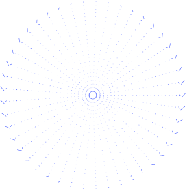
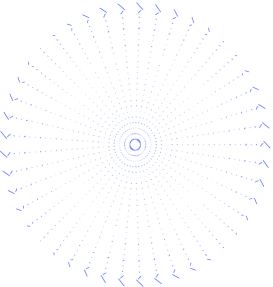
Figure 1: Pure $B$ modes with non-zero projection into the range of $\bm{W}_{-}$, for band limited $E$ with $\ell_{\text{max}}=300$. The modes are for an azimuthally symmetric patch of sky with where $\theta_{\text{max}}=20^{\circ}$, and have $m=1$ and $m=2$.

For band limited skies one can use knowledge of the band limit to use the information from the modes with non-zero eigenvalues of $\bm{W}_{-}$. However in practice the $E$ polarization is effectively non-band limited as far as extracting the large scale $B$ signal is concerned. Thus one needs to find modes which lie in the null-space $\bm{W}_{-}$ to extract pure B modes. Note that it is the non-band limitedness of $E$ which implies inevitable loss due to mode separation, even in the limit of zero noise.

Extracting low multipoles

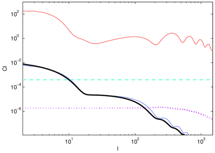
Figure 2: Typical $C_{l}$ for a concordance model with a reionization optical depth of $\tau=0.17$. The top line shows the scalar $E$-mode power spectrum, thick and thin solid lines show tensor $B$ and $E$ power spectra at an amplitude where tensors contribute about 1/10th of the large scale temperature anisotropy ($A_{T}=4\times 10^{-10}$). The dashed line gives an indication of the noise level with Planck, the dotted line show the $B$ spectrum due to gravitational lensing of the scalar $E$ signal. The detailed shape of the curves on large scales depends on the reionization history.

In the case where the E signal is effectively non-band limited, but we observe only a finite number $n$ of pseudo-harmonics with $\ell\leq\ell_{\text{max}}$, a pure $B$ mode $\mathbf{e}^{\dagger}\tilde{\mathbf{B}}$ can be extracted by finding a vector $\mathbf{e}$ lying in the left null space of $\bm{W}_{-}^{\infty}$, where $\bm{W}_{-}^{\infty}$ is in general an $n\times\infty$ matrix, coupling in $E$ on all scales. This requires that

$$|\mathbf{e}^{\dagger}\bm{W}_{-}^{\infty}|^{2}=\mathbf{e}^{\dagger}(\bm{W}_{+}-\bm{W}_{+}^{\infty}\bm{W}_{+}^{\infty}{}^{\dagger})\mathbf{e}=0$$ (34)

where here the $\bm{W}_{+}$ is the Hermitian square $n\times n$ matrix, $\bm{W}_{+}^{\infty}=(\bm{W}_{+},\bm{X})$ and $\bm{X}$ is $n\times\infty$. For a supported mode with $\bm{W}_{+}\mathbf{e}=\mathbf{e}$ this criterion is satisfied because $|\mathbf{e}^{\dagger}\bm{W}_{+}^{\infty}|\geq|\mathbf{e}^{\dagger}\bm{W}_{+}|$ and $|\mathbf{e}^{\dagger}\bm{W}_{-}^{\infty}|^{2}$ must be positive or zero. Note that $\bm{W}_{+}\mathbf{e}=\mathbf{e}$ is sufficient but not necessary for $|\mathbf{e}^{\dagger}\bm{W}_{-}^{\infty}|$ to vanish — in the case of an azimuthal patch there is a left null space for finite $\ell_{\text{max}}$ even though there are no vectors satisfying $\bm{W}_{+}\mathbf{e}=\mathbf{e}$ (see Appendix A). However in general, without including information up to the band limit of the data or special symmetries, this cannot be done. The idea here is to perform E/B separation for the low multipoles without including data up to the band limit (which due to the $\ell_{\text{max}}^{6}$ scaling would be infeasible with current computers for general patches).

In general for finite $n$ there will be no fully supported modes, however for an eigenvector $\mathbf{e}$ of $\bm{W}_{+}$ with $\bm{W}_{+}\mathbf{e}=(1-\epsilon)\mathbf{e}$ it follows that $|\mathbf{e}^{\dagger}\bm{W}_{-}^{\infty}|^{2}={\cal O}(\epsilon)$. In other words, approximately pure $B$ modes are simply the well supported modes. Note that $\bm{W}_{-}\mathbf{e}\approx 0$ is necessary but not sufficient since it does not ensure there is no coupling to power from $E$ on scales with $\ell>\ell_{\text{max}}$ in general.

The signal variance of $\mathbf{e}^{\dagger}\tilde{\mathbf{B}}$ is given by

$$\langle|\mathbf{e}^{\dagger}\tilde{\mathbf{B}}|^{2}\rangle=W^{+}_{l}C^{BB}_{l}+W^{-}_{l}C^{EE}_{l}$$ (35)

where

$$W^{+}_{l}\equiv\sum_{m}|(\mathbf{e}^{\dagger}\bm{W}_{+})_{lm}|^{2}\quad\quad W^{-}_{l}\equiv\sum_{m}|(\mathbf{e}^{\dagger}\bm{W}_{-})_{lm}|^{2}.$$ (36)

The scalar contribution to the $C^{EE}_{l}$ power spectrum is typically between $1\text{--}100$ times larger than $C^{BB}_{l}$ for $\ell\lesssim 100$ and levels of B detectable by Planck (see Fig. 2), and remains of the same order of magnitude up to $\ell\sim 2000$. Taking $C^{EE}_{l}\sim\text{const}$ the E contribution to the variance is $\sim|\mathbf{e}^{\dagger}\bm{W}_{-}^{\infty}|^{2}$, thus we require $\epsilon\ll 0.01$ for clean separation of B. However there is little point removing E to levels much lower than the experimental noise, so for noise limited observations larger values of $\epsilon$ could be used.

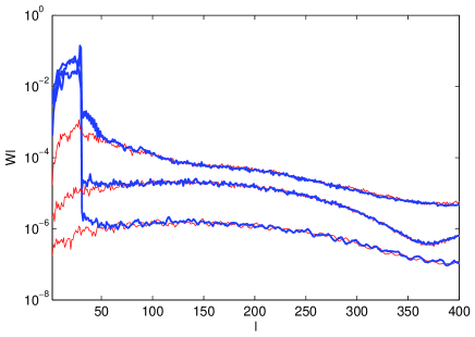
Figure 3: The functions $W_{l}^{+}$ (thick lines, the coupling to B) and $W_{l}^{-}$ (thin lines, the coupling to E) giving the contributions to the variance for some nearly pure B modes with various degrees of support ($\epsilon=\{0.1,0.01,0.001\}$, top to bottom), constructed with $\ell_{\text{max}}=30$ and the asymmetric sky cut discussed in the text.

In Fig. 3 we show a few window functions $W^{+}_{l}$ and $W^{-}_{l}$ for nearly pure B modes, using $\ell_{\text{max}}=30$ and the realistic cut discussed in the next section. This low value of $\ell_{\text{max}}=30$ is not sufficient to extract many well supported modes (there is only one with $\epsilon=0.001$), however it allows us to compute the rectangular matrices $\bm{W}_{+}$ and $\bm{W}_{-}$ up to much higher $\ell$ in order to explicitly show the coupling of higher multipoles as a function of the choice of $\epsilon$. The expected behavior is demonstrated in the figure, with small values of $\epsilon$ effectively removing the coupling to E on all scales.

IV Examples

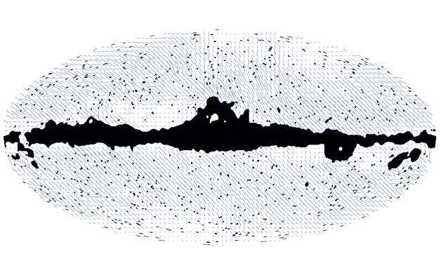
Figure 4: The nearly pure well supported B mode with maximal signal for a $\tau\sim 0.12$ reionization model, $\ell_{\text{max}}=150$, $\epsilon=0.001$ and the ‘kp2’ sky cut discussed in the text. The Mollweide projection is used for the cut, but polarization orientations are not projected.

We now demonstrate explicitly the extraction of large scale B modes from a realistic non-symmetric sky cut, the ‘kp2’ cut used by the WMAP analysis Bennett et al. (2003). This excludes the galactic region, in addition to a number of other foreground sources, in total excluding about $15\%$ of the sky, and is shown as the solid area in Fig. 4. This may not be a good cut for polarized observations, but the cut is realistic in the sense that it does not have any artificial symmetries, and therefore is a reasonable test case for how B mode extraction can work in practice.

As shown in Fig. 2 the large scale reionization signal with $\ell\lesssim 10$ is large and has high signal to noise, at least if the optical depth really is $\gtrsim 0.1$. We use $\ell_{\text{max}}=150$, which is computationally tractable ($\sim 10\text{GB}$ of memory, few days of CPU time) and sufficient to get most of the large scale reionization power. The well supported mode with $\epsilon=0.001$ and maximal signal is shown in Fig. 4. With more effort (e.g. distributing the computation over a cluster or more efficient algorithms) it may be possible to push to $\ell_{\text{max}}\sim 300$, possibly enough to extract essentially all of the separable B modes due to primordial gravitational waves. This may be essential if the reionization turns out to be less significant, and of course resolving the shape of the magnetic power spectrum is a key check that the signal really is due to primordial tensor modes. Separation on smaller scales (e.g. as a consistency check, and for studying the lensing signal) would have to proceed on azimuthally symmetric cuts over clean regions of the sky with a number of cuts around foreground sources (see Appendix A), or rely on quadratic methods that work very well for estimating the separated power spectra on small scales.

Identifying the well supported modes is straightforward, and requires diagonalization of the Hermitian matrix $\bm{W}_{+}$,

$$\bm{W}_{+}=\bm{U}_{+}\bm{D}_{+}\bm{U}_{+}^{\dagger}.$$ (37)

Since we only need the well supported modes, in practice we only need to compute the eigenvectors with eigenvalues between $1-\epsilon$ and $1$, for some choice of $\epsilon$ and $\ell_{\text{max}}$. For large $\ell_{\text{max}}$ there are $\sim f_{\text{sky}}\ell_{\text{max}}^{2}$ such modes, where $f_{\text{sky}}$ is the fraction of the sky included in the window. For less large $\ell_{\text{max}}$ a significant fraction of modes will only be partially supported; losing the subset of these modes that are not contaminated with $E$ is the price we pay for a computationally tractable analysis with manageable $\ell_{\text{max}}$. The well supported eigenvectors define a reduced column-orthogonal matrix $\tilde{\bm{U}}_{+}$ which projects the cut-sky harmonics into the space of well supported nearly-pure B modes:

$$\mathbf{X}_{B}\equiv\tilde{\bm{U}}_{+}^{\dagger}\tilde{\mathbf{B}}\approx\tilde{\bm{U}}_{+}^{\dagger}\mathbf{B}.$$ (38)

A map of the nearly pure B modes can then be constructed using the harmonics $\mathbf{B}^{\prime}=\tilde{\bm{U}}_{+}\tilde{\bm{U}}_{+}^{\dagger}\tilde{\mathbf{B}}$. Note that though computing $\tilde{\bm{U}}_{+}$ is time consuming for large $\ell_{\text{max}}$, once this has been done for a particular cut, construction of B maps for different realizations is computationally fast.

In Fig. 5 we show the construction of a B map for a simple simulation without noise. The recovered B map is not the same as the input map since we are only using $\ell_{\text{max}}=150$, and some modes are lost due to E/B separation. However it is clear than many of the large scale features are present in the recovered map, and that the method works usefully well.

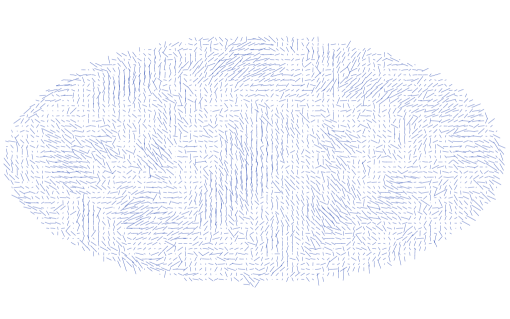
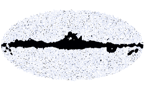
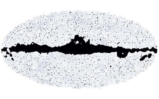
Figure 5: Simulation of noise-free well supported B mode extraction ($\ell_{\text{max}}=150$, $\epsilon=0.001$) for the ‘kp2’ cut. Top: input B map due to tensor modes. Middle: the observed cut sky including E polarization from scalar and tensor modes ($A_{T}=4\times 10^{-10}$). Bottom: the reconstructed well supported nearly pure B modes. Line orientations show the polarization direction, line lengths show the magnitude. For each map the lengths are independently normalized. The sky is represented in the Mollweide projection (but polarization orientations are not projected), and the beam size is half a degree.

Noise

In general there will be anisotropic and correlated noise on the polarization measurements. The E/B separation methods we discussed give E/B clean separation of the signal, however any interpretation of the separated modes would have to carefully model the actual noise properties in the observation under consideration. In general the E and B modes will have complicated noise correlations. However in the idealized case of isotropic uncorrelated noise on the Stokes’ parameters the noise properties are straightforward Lewis et al. (2002). In particular the well supported E and B modes will also have uncorrelated isotropic noise

$$\langle\mathbf{X}_{B}\mathbf{X}_{B}^{\dagger}\rangle_{N} \approx \langle\tilde{\bm{U}}_{+}^{\dagger}\mathbf{B}\mathbf{B}^{\dagger}\tilde{\bm{U}}_{+}\rangle_{N}\approx\langle\mathbf{X}_{E}\mathbf{X}_{E}^{\dagger}\rangle_{N}\propto\bm{I}$$

$$\langle\mathbf{X}_{B}\mathbf{X}_{E}^{\dagger}\rangle_{N} \approx \langle\tilde{\bm{U}}_{+}^{\dagger}\mathbf{B}\mathbf{E}^{\dagger}\tilde{\bm{U}}_{+}\rangle_{N}\approx 0.$$ (39)

The complications introduced by correlated anisotropic noise do not effect the signal E/B separation, which is purely determined by the geometry of the sky cut. As the noise in a region inside the cut increases, some of the modes will become much more noisy. In the limit of infinite noise in this region, corresponding to an additional cut, these modes have zero signal to noise and can be removed. This removes combinations of E and B modes in such a way that the number of pure B modes that can be measured decreases, and new ambiguous modes (which are combinations of E and B with finite noise) are generated.

Detection by Planck?

Fig. 6 shows how the E/B separation method performs with regards to the detection probability for magnetic polarization due to tensor modes, taking a simple model of the Planck satellite as a test case (assuming isotropic Gaussian noise, that foregrounds can be subtracted accurately outside the cut region, and systematics are negligible). We assume the primordial tensor modes are Gaussian with scale invariant power spectrum, with $A_{T}$ being the variance of the transverse traceless part of the metric tensor, and that other cosmological parameters are well known.

The approximate method applied to the asymmetric cut does not perform quite as well as an optimal analysis with an azimuthally symmetric cut, but the difference is not that large — equivalent to reducing a $99\%$ confidence detection to about $95\%$. The asymmetric cut is not expected to perform as well because it increases the area adjacent to a boundary and hence the number of ambiguous modes (though the approximate result may be improved slightly by taking larger $\ell_{\text{max}}$). The plot also shows the result of applying the non-exact method (retaining just the well supported modes) to the azimuthally symmetric cut, and shows that the results are almost identical to performing the exact separation in this case. In the exact azimuthal analysis the result is almost completely insensitive to $\ell_{\text{max}}$, with $\ell_{\text{max}}=30$ results lying on top of those shown. This is because of the small number of large signal to noise modes on large scales for a significant optical depth to reionization. In the asymmetric case much larger $\ell_{\text{max}}$ is needed to obtain well supported modes.

For $\tau\gtrsim 0.1$ it is clear that Planck should have a good chance of detecting tensor amplitudes $A_{T}\gtrsim 10^{-10}$, corresponding to an energy scale $V^{1/4}\gtrsim 10^{16}\text{GeV}$ at horizon crossing during inflation. The sensitivity to tensor magnetic modes however depends on the reionization optical depth, as shown in Fig. 7. If the optical depth turns out to be at the lower end, the asymmetric cut with $\ell_{\text{max}}\sim 150$ would not perform so well compared to the exact azimuthal case since there would be significant power on smaller scales, requiring $\ell_{\text{max}}\gg 100$ to construct all the well supported modes.

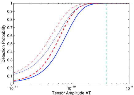
Figure 6: Tensor magnetic polarization detection probabilities for Planck at a confidence of 99 per cent (thick lines) and 95 per cent (thin lines) using nearly pure B modes. Solid lines are for the ‘kp2’ cut using $\ell_{\text{max}}=150$ and $\epsilon=0.001$. Dashed lines are for exact E/B separation with an azimuthally symmetric cut (with the same $f_{\text{sky}}$) and $\ell_{\text{max}}=250$. Dotted lines are for the azimuthally symmetric cut, but using the well supported modes method ($\ell_{\text{max}}=150$ and $\epsilon=0.001$). For all lines we assume isotropic $C_{\text{noise}}=4.1\times 10^{-4}\mu K^{2}$ and a reionization optical depth $\tau\sim 0.12$. The vertical dashed line shows the tensor amplitude that would contribute about 1/10th of the large scale temperature anisotropy (approximately the limit that can be set without using polarization).

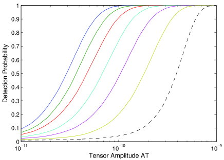
Figure 7: The probabilities for 99 per cent confidence detections of magnetic polarization with a simple model of Planck, for reionization optical depths $\tau=\{0.2,0.17,0.14,0.11,0.08,0.05\}$ (left to right) assuming sharp reionization. The dotted line shows the result if there is no foreground-distinguishable B mode signal at $l<30$. Exact B mode separation is used with an azimuthally symmetric galactic cut with $f_{\text{sky}}=0.85$.

V Conclusion

We have demonstrated explicitly that E/B separation is possible on large scales for realistic non-symmetric sky cuts. If the reionization optical depth is large almost all the detection significance for tensor modes would come from the very largest scales, where mode mixing is most important. We showed that these modes can be separated in a computationally tractable way by retaining only the well supported modes. The ambiguous modes that cannot be separated will be dominated by the E signal if the noise is low, and whilst useful for analysis of the E polarization would not add significantly to a full likelihood analysis for magnetic polarization.

With map-level separation one can also in principle study the full distribution of the B signal, for example testing for Gaussianity. Analysing a pure B map is essentially the same as analysing a temperature map, and much more more straightforward and conceptually cleaner than doing a full joint analysis. For noise limited observations, when the loss of ambiguous modes loses a significant amount of information, an analysis with E/B separated variables still provides a valuable cross-check on results from a full joint analysis, and may help to isolate systematics.

Appendix A Circular boundaries

For a circular boundary at constant latitude $\theta=\Theta$ (i.e. the boundary of an azimuthal patch), modes with different $m$ decouple, $\bm{W}_{-}$ is block diagonal, and modes with different $m$ can be handled separately. The $\bm{W}_{-}$ surface boundary integral evaluates to Lewis et al. (2002)

$$W_{-(lm)(l^{\prime}m^{\prime})}=-\frac{m\delta_{mm^{\prime}}}{2|m|}\left[u_{l}(m)u_{l^{\prime}}^{\ast}(m)+v_{l}(m)v_{l^{\prime}}^{\ast}(m)\right]_{\Theta},$$ (40)

where the vectors

$$u_{l}(m) \equiv \sqrt{\frac{(l-2)!}{(l+2)!}}\sqrt{8|m|\pi}\sin\theta\frac{\text{d}}{\text{d}\theta}\left(\frac{Y_{lm}}{\sin\theta}\right)$$ (41)

$$v_{l}(m) \equiv \sqrt{\frac{(l-2)!}{(l+2)!}}\frac{\sqrt{8|m|\pi(m^{2}-1)}}{\sin\theta}Y_{lm}$$ (42)

for $l\geq 2$ and some arbitrary $\phi$. In the $\ell_{\text{max}}\rightarrow\infty$ limit this is the spectral decomposition ($v_{l}(m)$ and $u_{l}(m)$ are normalized and orthogonal), which follows from the results:

$$\sum_{l=|m|}^{\infty}\frac{(l-2)!}{(l+2)!}|Y_{lm}|^{2}=\frac{\sin^{2}\theta}{8|m|\pi(m^{2}-1)}$$ (43)

$$\sum_{l=|m|}^{\infty}\frac{(l-2)!}{(l+2)!}Y_{lm}^{*}\sin\theta\frac{\text{d}}{\text{d}\theta}\left(\frac{Y_{lm}}{\sin\theta}\right)=0$$ (44)

for $|m|\geq 2$, and

$$\sum_{l=\max(2,|m|)}^{\infty}\frac{(l-2)!}{(l+2)!}\left|\sin\theta\frac{\text{d}}{\text{d}\theta}\left(\frac{Y_{lm}}{\sin\theta}\right)\right|^{2}=\frac{1}{8|m|\pi}$$ (45)

for $|m|\geq 1$. In this limit the eigenvalues are $-{\textstyle\frac{1}{2}}m/|m|$, a special case of the general analysis given in section II. For a single circular boundary and finite $\ell_{\text{max}}$ there are at most two non-zero eigenvalues per $m$, with one for $|m|=1$ and none for $m=0$.

The azimuthal case has the nice property that even if $\tilde{\mathbf{E}}$ and $\tilde{\mathbf{B}}$ are only available for finite $\ell_{\text{max}}$ one can project out exactly the cross-contamination on all scales. The matrix $\bm{W}_{-}$ truncated at a finite number of rows (but retaining an unlimited number of columns) can be written as

$$\bm{W}_{-}=\bm{U}_{-}\bm{D}_{-}\bm{V}_{-}^{\dagger}$$ (46)

where $\bm{U}_{-}$ is a column unitary matrix with at most two columns per $m$, and hence the range of $\bm{W}_{-}$ can be projected out using

$$\bm{P}_{-} \equiv\bm{I}-\bm{U}_{-}\bm{U}_{-}^{\dagger}$$ (47)

so that

$$\bm{P}_{-}\tilde{\mathbf{E}} =\bm{P}_{-}\bm{W}_{+}\mathbf{E}\quad\quad\quad\bm{P}_{-}\tilde{\mathbf{B}} =\bm{P}_{-}\bm{W}_{+}\mathbf{B}$$ (48)

losing at most two modes per $m$ (per boundary). The matrix $\bm{U}_{-}$ can in practice be constructed for each $m$ by normalization and orthogonalization (e.g. using a SVD) of the two vectors $u_{l}(m)$ and $v_{l}(m)$ (which are no longer orthogonal or normalized for finite $\ell_{\text{max}}$). This projection is equivalent to the procedure of projecting out the non-zero eigenvalues of $\bm{W}_{-}$ in Ref. Lewis et al. (2002), for $|m|\leq\ell_{\text{max}}-2n$, where $n$ is the number of boundaries. If $\bm{W}_{-}$ is smaller than it’s range due to a finite $\ell_{\text{max}}$ (i.e. for $|m|>\ell_{\text{max}}-2n$) the zero eigenvalues $\bm{W}_{-}$ do not correspond to separated modes.

Two maps consisting of pure $E$ and pure $B$ can be constructed simply from

$$\tilde{\mathbf{E}}^{\prime} =(\bm{I}-\bm{U}_{-}\bm{U}_{-}^{\dagger})\tilde{\mathbf{E}},\quad\ \tilde{\mathbf{B}}^{\prime}= 0\quad(\text{pure E})\quad$$ (49)

$$\tilde{\mathbf{B}}^{\prime} =(\bm{I}-\bm{U}_{-}\bm{U}_{-}^{\dagger})\tilde{\mathbf{B}},\quad\tilde{\mathbf{E}}^{\prime}= 0\quad(\text{pure B}).\quad$$ (50)

If desired a map of the ambiguous modes can also be constructed from the remaining modes. The separation is computationally trivial in the azimuthal case due to the separability in $m$, and is possible up to the resolution of the experiment (typically $\ell_{\text{max}}>10^{3}$).

For $n$ co-axial circular boundaries one looses up to $4n(\ell_{\text{max}}-n)$ modes due to the E/B separation, and the separation remains exact and separable in $m$. For non-co-axial boundaries exact separation is still possible, even though modes with different $m$ are mixed due to the rotation (i.e. with the Wigner-D matrices $D^{l}_{mm^{\prime}}$). This is because the coupling matrix $\bm{W}_{-}$ for the entire sky made up of a set of non-intersecting cuts can be written as a finite sum of coupling matrices $\bm{W}_{-}$ each with finite range, and therefore itself has finite range which can be projected out exactly. Thus it is still possible to perform exact E/B separation at finite $\ell_{\text{max}}$ with azimuthal cuts containing a finite number of non-intersecting circular cuts around foreground sources.

To extract a set of E and B modes for likelihood evaluation one can proceed following Ref. Lewis et al. (2002). We briefly review the method here with one minor enhancement. First we diagonalize $\bm{W}_{+}$ (taking it to be square) and discard the badly supported modes, to write $\bm{W}_{+}\approx\tilde{\bm{U}}_{+}\tilde{\bm{D}}_{+}\tilde{\bm{U}}_{+}^{\dagger}$ so

$$\tilde{\bm{D}}^{-1/2}_{+}\tilde{\bm{U}}_{+}^{\dagger}\tilde{\mathbf{E}}\approx\tilde{\bm{D}}^{1/2}_{+}\tilde{\bm{U}}_{+}^{\dagger}\mathbf{E}+i\tilde{\bm{D}}^{-1/2}_{+}\tilde{\bm{U}}_{+}^{\dagger}\bm{W}_{-}\mathbf{B}$$ (51)

$$\tilde{\bm{D}}^{-1/2}_{+}\tilde{\bm{U}}_{+}^{\dagger}\tilde{\mathbf{B}}\approx\tilde{\bm{D}}^{1/2}_{+}\tilde{\bm{U}}_{+}^{\dagger}\mathbf{B}-i\tilde{\bm{D}}^{-1/2}_{+}\tilde{\bm{U}}_{+}^{\dagger}\bm{W}_{-}\mathbf{E}.$$ (52)

Then we do the diagonalization

$$\tilde{\bm{D}}^{-1/2}_{+}\tilde{\bm{U}}_{+}^{\dagger}\bm{W}_{-}\tilde{\bm{U}}_{+}\tilde{\bm{D}}^{-1/2}_{+}=\bm{U}_{-}\bm{D}_{-}\bm{U}_{-}^{\dagger}$$ (53)

and construct the matrix $\tilde{\bm{U}}_{-}$ by deleting the columns of $\bm{U}_{-}$ corresponding to non-zero diagonal elements of $\bm{D}_{-}$. It follows from the Hermiticity of $\bm{W}_{-}$ that $\tilde{\bm{U}}_{-}$ is made up of vectors in the left null-space of the mode-mixing matrix $\tilde{\bm{D}}^{-1/2}_{+}\tilde{\bm{U}}_{+}^{\dagger}\bm{W}_{-}$. The pure E and B modes are then given by

$$\tilde{\bm{U}}_{-}^{\dagger}\tilde{\bm{D}}^{-1/2}_{+}\tilde{\bm{U}}_{+}^{\dagger}\tilde{\mathbf{E}} \approx \tilde{\bm{U}}_{-}^{\dagger}\tilde{\bm{D}}^{1/2}_{+}\tilde{\bm{U}}_{+}^{\dagger}\mathbf{E}$$ (54)

$$\tilde{\bm{U}}_{-}^{\dagger}\tilde{\bm{D}}^{-1/2}_{+}\tilde{\bm{U}}_{+}^{\dagger}\tilde{\mathbf{B}} \approx \tilde{\bm{U}}_{-}^{\dagger}\tilde{\bm{D}}^{1/2}_{+}\tilde{\bm{U}}_{+}^{\dagger}\mathbf{B}.$$ (55)

For isotropic uncorrelated noise these modes also have isotropic and uncorrelated noise. This method is equivalent to that presented in Ref. Lewis et al. (2002) but slightly faster as it replaces the SVD of the $\tilde{\bm{D}}^{-1/2}_{+}\tilde{\bm{U}}_{+}^{\dagger}\bm{W}_{-}$ coupling matrix with a faster diagonalization of a smaller Hermitian matrix by using the Hermiticity of $\bm{W}_{-}$. Note that as mentioned above one should only include modes with $|m|\leq\ell_{\text{max}}-2n$, though in practice for galactic cuts these modes are badly supported anyway. The coupling matrices for an azimuthal cut can be computed efficiently using the results given in the appendix of Ref. Lewis et al. (2002).

References

- Kamionkowski et al. (1997) M. Kamionkowski, A. Kosowsky, and A. Stebbins, Phys. Rev. D55, 7368 (1997), eprint astro-ph/9611125.
- Zaldarriaga and Seljak (1997) M. Zaldarriaga and U. Seljak, Phys. Rev. D55, 1830 (1997), eprint astro-ph/9609170.
- Hu et al. (1998) W. Hu, U. Seljak, M. White, and M. Zaldarriaga, Phys. Rev. D57, 3290 (1998), eprint astro-ph/9709066.
- Knox and Song (2002) L. Knox and Y.-S. Song, Phys. Rev. Lett. 89, 011303 (2002), eprint astro-ph/0202286.
- Okamoto and Hu (2003) T. Okamoto and W. Hu, Phys. Rev. D67, 083002 (2003), eprint astro-ph/0301031.
- Hirata and Seljak (2003) C. M. Hirata and U. Seljak, Phys. Rev. D68, 083002 (2003), eprint astro-ph/0306354.
- Seljak et al. (1997) U. Seljak, U.-L. Pen, and N. Turok, Phys. Rev. Lett. 79, 1615 (1997), eprint astro-ph/9704231.
- Pogosian et al. (2003) L. Pogosian, S. H. H. Tye, I. Wasserman, and M. Wyman, Phys. Rev. D68, 023506 (2003), eprint hep-th/0304188.
- Lewis (2004a) A. Lewis (2004a), eprint astro-ph/0406096.
- Lewis (2004b) A. Lewis (2004b), eprint astro-ph/0403583.
- Hu et al. (2003) W. Hu, M. M. Hedman, and M. Zaldarriaga, Phys. Rev. D67, 043004 (2003), eprint astro-ph/0210096.
- Crittenden et al. (2002) R. G. Crittenden, P. Natarajan, U. Pen, and T. Theuns, Astrophys. J. 568, 20 (2002), eprint astro-ph/0012336.
- Chon et al. (2004) G. Chon, A. Challinor, S. Prunet, E. Hivon, and I. Szapudi, Mon. Not. Roy. Astron. Soc. 350, 914 (2004), eprint astro-ph/0303414.
- Kogut et al. (2003) A. Kogut et al., Astrophys. J. Suppl. 148, 161 (2003), eprint astro-ph/0302213.
- Lewis et al. (2002) A. Lewis, A. Challinor, and N. Turok, Phys. Rev. D65, 023505 (2002), eprint astro-ph/0106536.
- Bunn et al. (2003) E. F. Bunn, M. Zaldarriaga, M. Tegmark, and A. de Oliveira-Costa, Phys. Rev. D67, 023501 (2003), eprint astro-ph/0207338.
- Zaldarriaga (2001) M. Zaldarriaga, Phys. Rev. D64, 103001 (2001), eprint astro-ph/0106174.
- Park and Ng (2003) C.-G. Park and K.-W. Ng (2003), eprint astro-ph/0304167.
- Pen (2004) U.-L. Pen, New Astron. 9, 417 (2004), eprint astro-ph/0305387.
- Mortlock et al. (2002) D. J. Mortlock, A. D. Challinor, and M. P. Hobson, MNRAS 330, 405 (2002), eprint astro-ph/0008083.
- Bennett et al. (2003) C. Bennett et al. (2003), eprint astro-ph/0302208.
- Gorski et al. (1998) K. M. Gorski, E. Hivon, and B. D. Wandelt, in Proceedings of the MPA/ESO Conferece on Evolution of Large-Scale Structure, edited by A. Banday, R. Sheth, and L. D. Costa (PrintPartners Ipskamp, Enschede, NL, 1998), pp. 37–42, eprint astro-ph/9812350.