VLBI observations of T Tauri South

We report observations of the T Tauri system at 8.4 GHz with a VLBI array comprising the VLBA, VLA and Effelsberg 100m telescopes. We detected a compact source offset approximately 40 mas from the best infrared position of the T Tau Sb component. This source was unresolved, and constrained to be less than 0.5 mas in size, corresponding to 0.07 AU or 15 R_⊙ at a distance of 140 pc. The other system components (T Tau Sa, T Tau N) were not detected in the VLBI data. The separate VLA map contains extended flux not accounted for by the compact VLBI source, indicating the presence of extended emission on arcsecond scales. The compact source shows rapid variability, which together with circular polarization and its compact nature indicate that the observed flux arises from a magnetically-dominated region. Brightness temperatures in the MK range point to gyrosynchrotron as the emission mechanism for the steady component. The rapid variations are accompanied by dramatic changes in polarization, and we record an at times 100% polarized component during outbursts. This strongly suggests a coherent emission process, most probably an electron cyclotron maser. With this assumption it is possible to estimate the strength of the local magnetic field to be 1.5-3 kilogauss.

1 Introduction

Classical T Tauri stars are still in the process of contraction towards the zero age main sequence, and continue to accrete material through circumstellar disks. The inner part of the disk is believed to be truncated by strong magnetic fields anchored on the star, and the disk material may then be channeled down field lines onto the stellar surface. The accretion process is thought to be linked to the launch of highly-collimated jets from the inner disk or magnetosphere. Evidence for this scenario comes primarily from observations of infalling material close to the star, and measurements of kilogauss strength photospheric fields for a few objects (Basri, Marcy & Valenti, 1992, Guenther et al. 1999, Johns-Krull et al. 1999a, b).

In the solar corona, magnetic fields lead to non-thermal radio emission by various processes caused by accelerated electrons (see e.g. review by Benz 2002). Particle acceleration is a basic process in flares, probably initiated by reconnection of field lines in active regions. Some of these accelerated particles (those with energies typically 20-100 keV), can ablate material from the solar surface, leading to the emission of soft X-rays. In the solar interior, free magnetic energy is built up by subsurface convection. The fields envisaged for T Tauri stars probably also arise due to convection, but are thought to have typically a larger length scale than those of the Sun, and probably more resemble the large-scale fields thought to exist in RS CVn systems (see e.g. White 2000 and references therein). Nevertheless, the solar analogy is instructive in phenomena such as flares, where the same physical processes lie behind the observed behaviour. Disks may be important for magnetic energy release in very young stars since, if the inner disk and the stellar surface are not rotating in phase, then magnetic fields anchored at both sites will be wound up and transfer angular momentum between star and disk (Montmerle et al. 2000). This will also lead to magnetic reconnection and energy release after a sufficient amount of rotation (Hayashi, Shibata & Matsumoto, 1996). Such processes may also play a role in driving jets and bipolar outflows.

T Tauri itself is a highly complex multiple system. The northern optical source (hereafter T Tau N) was found to have an infrared companion, T Tau S, approximately 0.7^′′ to the south (Dyck, Simon & Zuckerman, 1982, Ghez et al. 1991). T Tau S has been found also to be binary, with a separation of approximately 100 mas (Koresko 2000, Köhler, Kasper & Herbst 2000). Subsequent observations of the two southern sources (hereafter referred to as Sa for the eastern object and Sb for the western) revealed relative motion, which could be a segment of an orbit (Duchêne, Ghez & McCabe 2002). K-band spectroscopy by these authors reveals that T Tau Sb has spectral type M, whereas T Tau Sa is a continuum source, having an SED probably peaking at IR wavelengths. The IR observations show that T Tau Sa remains nearly stationary, indicating that it is the most massive object in the southern system. Johnston et al (2003) observed the T Tau system at 2cm with the VLA in ‘A’ configuration between 1983 and 2001. They detected both the northern and southern components. By assuming that the southern radio component could be identified with the M star, they were able to determine an orbit for the Sa-Sb pair and hence estimate the total mass of the southern system to be 5.3 $M_{\odot}$.

Other radio observations at high resolution have revealed important polarization and variability features at all observed wavelengths (e.g. Philips, Lonsdale & Feigelson, 1993, at 18 cm using VLBI and VLA; Skinner & Brown, 1994, at 2, 3.6 and 6 cm using the VLA in A configuration; Ray et al., 1997, at 6 cm using MERLIN). T Tau S dominates the emission at radio frequencies. Skinner & Brown found T Tau S to have a falling spectrum and circular polarization, suggestive of a magnetic origin for the emission. They also observed a 50% flux increase, accompanied by a reversal in polarization, from left- to right-handed. Ray et al. (1997) claim to have detected polarized emission associated with T Tau S, with regions of left and right handed circular polarization on either side of the star offset from one another by some 0.15^′′ along a northwest-southeast axis. This was interpreted as emission from a magnetically-threaded outflow, with oppositely-directed field lines leading to opposite observed circular polarization. On a slightly larger scale, White (2000) reported high resolution VLA observations showing extended structure to the northeast of the southern component.

It has been suggested that T Tau N is seen roughly pole on to the line of sight, based on a comparison of the photometric period, the stellar radius and the rotational broadening of photospheric lines. This suggestion has been used to explain the discrepant extinction between T Tau N and S, with the northern component viewed through a cavity in the envelope cleared by the outflow (Momose et al., 1996). The jet from the T Tau S system, however, appears to lie nearly in the plane of the sky (van Langevelde et al. 1994), a view reinforced by modelling of the scattered optical and NIR light surrounding the stars (Wood et al., 2001). If this is so, the T Tau components must have strongly misaligned rotation axes.

In this paper, we present VLBI observations of the T Tau S system. Our main intention was to probe the inner regions of the system in order to study the collimating mechanism of the jet at higher resolution than achieved by Ray et al. We serendipitously observed the T Tau S system undergo two strong flux increases, accompained by changes in circular polarization. The extra flux in the second of these brightenings appears to be 100% circularly polarized, something which to our knowledge has never been seen previously in an accreting pre-main sequence system. The spatial resolution offered by the VLBI interferometry network should enable us to separate the two components of T Tau S, but the maps reveal only one source. We identify our detection as being T Tau Sb, the M star of the southern binary system. We also fail to detect T Tau N at high resolution, despite detecting it clearly with the VLA. In the further discussions, we will refer to the entire T Tau S system when the single components are not explicitly named.

2 The observations

The observations were conducted on December 15th, 1999. All times referred to are measured from $0^{h}$UT on this date. Ten VLBA stations were used, together with the Effelsberg 100m telescope and the phased VLA in ‘B’ configuration. The observing frequency was 8.4GHz (3.6cm, X band). The bright quasars J0431+1731 and J0357+2319, lying at 3^∘ and 7^∘ from T Tau respectively, were used as phase calibrators. Since astrometry was not the primary goal of the experiment, phase calibrators with positions determined from geodectic observations were not required. The two phase calibrators used had positions determined from VLBA survey observations and were disposed along a line with T Tau between them. The phase solutions on both of them should have allowed us to get precise phase solutions at the target location. Unfortunately the observing schedule contained too few scans on the secondary calibrator making the signal to noise ratio on J0357+2319 too bad to get reliable phase solutions. J0357+2319 was therefore used to check the quality of the phase referencing. Hybrid maps of J0357+2319 were produced showing an offset from the phase center of approximately 20 mas. Since T Tau S lies between the two calibrators, we can be sure that the astrometric accuracy at the T Tau S position is at least 20 mas, and probably better in proportion to the relative proximity of T Tau S to the primary phase calibrator. This will be discussed further in Section 3.1.

The T Tau S observations were scheduled in 9 blocks consisting of three alternations between T Tau S (3 minutes) and J0431+1731 (2 minutes), with one scan on J0357+2319 (2 minutes) at the beginning and the end of each block. The total observation time on T Tau S was about 1.5 hours. The blocks were separated by gaps of approximately one hour, during which we observed another two targets which are not discussed in the present paper.

3 Results

3.1 Source positions

Table 1: Source positions. All positions have been proper motion corrected to the observation epoch, as described in the text, but no attempt has been made to correct for orbital motion. The uncertainty in the last digit is given in parentheses. References: (a) Hipparcos position proper motion corrected to observation epoch with Hipparcos proper motion. (b) Offset from T Tau N given by Duchêne et al. (2002). (c) Offset from T Tau Sa given by Köhler et al. (2000). (d) Johnston et al. (2003).

Source	$\alpha$	$\delta$	Ref
T Tau N (opt)	4h 21m 59s.434 (1)	19∘ 32′ 06′′.429 (14)	a
T Tau Sa (IR)	4h 21m 59s.435 (1)	19∘ 32′ 05′′.727 (14)	b
T Tau Sb (IR)	4h 21m 59s.427 (1)	19∘ 32′ 05′′.722 (14)	b
T Tau Sb (IR)	4h 21m 59s.429 (1)	19∘ 32′ 05′′.704 (14)	c
T Tau S (2cm)	4h 21m 59s.4242 (1)	19∘ 32′ 05′′.732 (3)	d
T Tau S (VLBI)	4h 21m 59s.4263 (14)	19∘ 32′ 05′′.730 (20)

The VLBI map of the T Tau S field is plotted in Figure 1. A single pointlike source can be seen at position $\alpha=4^{h}\leavevmode\nobreak\ 21^{m}\leavevmode\nobreak\ 59^{s}.4263$, $\delta=19^{\circ}\leavevmode\nobreak\ 32^{\prime}\leavevmode\nobreak\ 5^{\prime\prime}.730$ (equinox 2000). This position is epoch 1999.958, and has been corrected for parallax using the Hipparcos value of 5.66 mas. The astrometric accuracy was estimated from the position of the secondary calibrator J0357+2319 in the hybrid map compared to its expected position from the VLBA survey. The detected source was found to be offset 23 mas to the east and 17 mas to the south of the catalogue position. Assuming that this offset arises from a combination of position errors for the primary and secondary calibration sources, we adopt an uncertainty at the T Tau S position will be $\sqrt{2}\times$ 20 mas, or 14 mas. This uncertainty is indicated with a circle around the source in Figure 1.

We can compare the position of the VLBI source to the expected positions of T Tau Sa and Sb in the infrared from the recent literature. These positions are available as offsets from the IR position of T Tau N. We take as the fundamental reference position the Hipparcos position of T Tau N, which is determined in the V-band. The epoch of the Hipparcos observation was 1991.25. The Hipparcos proper motion of $\alpha=$15.45$\pm$1.88, $\delta=-12.48\pm 1.62$ mas yr^-1 was applied to correct the T Tau N position to the epoch of our observation. The standard error in the T Tau N position at the epoch of the observations is then $\Delta\alpha=$16.4 mas, $\Delta\delta=$14.1 mas, and is dominated by the error arising from the proper motion correction.

The IR observations of Duchêne et al. (2002) give positions for Sa and Sb as offsets from the IR position of T Tau N at epoch 2000.2. We have used these offsets to calculate the positions for Sa and Sb which are given in Table 1. The orbital motion of T Tau S about T Tau N was estimated by Roddier et al. (2000) who found that the position angle of T Tau S relative to T Tau N changed by $0^{\circ}.66$ yr^-1. This translates into 8 mas per year in a westward direction. Since Sa is the brightest component in the IR (by about 2.5 magnitudes in K), we assume that this represents motion of T Tau Sa around T Tau N, although the motion of the photocentre could be influenced by the motion of T Tau Sb around T Tau Sa. Since any motion between the epoch of our observation and that of Duchêne et al. would be small, we have not attempted to account for it in the position of Sa. This assumption is also made by Johnston et al, and their observations are consistent with orbital motion of T Tau Sb around a stationary (with respect to T  Tau N) T Tau Sa. The observation of the T Tau S system by Köhler et al. (2000) is closest in time to our observation (epoch 2000.17 as opposed to 1999.96), and so this is the position for T Tau Sb with which the VLBI source position should be principally compared.

Finally, in Table 1 we list the position of the southern 2cm source observed by Johnston et al. at epoch 2001.0531, which has been proper motion corrected to epoch 1999.958 using the proper motion reported for T Tau S by these authors.

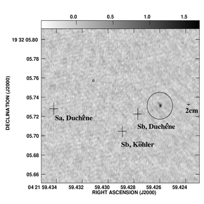
Figure 1: The VLBI T Tau S field. All positions have been proper motion corrected to the epoch of the VLBI observation but no attempt has been made to correct for possible orbital motion of components. A compact radio source is clearly seen. The circle plotted around this shows the estimated position uncertainty of the VLBI observation at 3.6cm. The positions of T Tau Sa and two positions for T Tau Sb, one from Köhler et al. and one from Duchêne et al., are marked with crosses. The size of the crosses show the position uncertainties. The 2cm radio position measured by Johnston et al at epoch 2001.0531 is shown as a small cross. Also marked (small circle) is the position expected for Sa if the radio source is taken to be Sb. The size of this small circle corresponds to the relative position uncertainty reported by Köhler (2000).

All the positions are listed in Table 1 and are shown in Figure 1, with the exception of T Tau N which lies outside the field. The T Tau Sa and Sb positions are marked with crosses, the sizes of which indicate the uncertainty in the positions which are dominated by the proper motion correction to the T Tau N position as previously noted. This component of the uncertainty is the same for Sa and Sb, and so the uncertainties shown for these sources are correlated.

The VLBI source in our map is closest to the position of T Tau Sb, and we make this identification, although there is a significant offset from the Köhler position. One way this might arise is because the T Tau N position is from the V-band Hipparcos observations, whereas the position of T Tau Sa relative to T Tau N by Duchêne et al. was determined in the near infrared. The presence of scattered light in the NIR may cause a discrepancy between the optical and NIR positions which then leads to a discrepancy between the T Tau S positions and the radio position. Possible orbital motion of the T Tau Sa+Sb system in the interval between our observations at epoch 1999.958 and the determination of the T Tau Sa position relative to T Tau N at epoch 2000.9 can be ruled out as an explanation, since the motion is both too small and in the wrong sense to account for the discrepancy.

We also show in Figure 1 the position expected for a radio source which could be identified as T Tau Sa, based on the hypothesis that the detected radio source is in fact T Tau Sb. This position is again determined from the Köhler et al. separation and position angle relative to the Sb position, and is marked with a small circle, the radius of which corresponds to the uncertainty in Köhler et al.’s position (there is no contribution here from the uncertainty in the T Tau N proper motion correction). It is clear that no radio source appears in the map at or near this position. We have also searched in the opposite position for a source corresponding to T Tau Sb based on the hypothesis that our detected source is in fact Sa, and this search was also unsuccessful.

A search was made in the VLBI map for other components of the system, namely T Tau N and the hypothetical source labeled T Tau R by Ray et al. (1997). As Johnston et al. (2003) we did not detect the supposed T Tau R component. The expected region of T Tau N lies outside the primary beam of the phased VLA, and so the search for this object lacks the most sensitive antenna. Phase problems may also degrade the image at such a large distance from the correlation centre. Despite the favorable RMS in the map (0.1 mJy), no sources were found anywhere in the region of T Tau N. No extended background flux was seen either. We conclude that the majority of the T Tau N flux is distributed over an area larger than about 20 mas, the resolution obtained at the shortest baseline available (Los Alamos-Pie Town, about 4M$\lambda$, see section 3.3).

     

Figure 2: Contour maps of the T Tau field from the VLA only data. The map on the left has been cleaned using the fitted beam of 1.15$\times$0.94^′′, whilst the map on the right has been cleaned using a restoring beam set to $0.5\times 0.5^{\prime\prime}$ to produce an artificial overresolution of the data. This allows T Tau N to be distinguished from T Tau S for the purposes of flux measurement. Positions are given as offsets from the position of the VLBI source, which is marked with a star. The position of T Tau N, T Tau Sa and T Tau Sb (from Duchêne et al., epoch 2000.2) are marked with crosses.

3.2 Fluxes and time variability

The VLA lightcurve is shown in Figure 3. The source brightened considerably during the observing run. Two large increases in flux occurred, one at around UT=7.15 hours and one at around UT=10.75 hours. Flaring behaviour can be seen at the beginning of the scan commencing at UT=7.14 hours. The upper right-hand panel of Figure 3 shows RCP and LCP behaviour separately. The polarization of the overall flux changes from about 5% LCP to about 6% RCP. The flare from UT=7.15 to 7.16 hours is almost totally right-hand polarized. This is shown at higher time resolution in the lower left-hand panel of Figure 3.

After UT=6 hours there is a long period of increased emission, with a slow decay, lasting until the second flux increase which is seen in the lightcurve beginning at UT=10.74 hours. Here, we did not see any sign of an initial flare within a scan (Figure 3, lower right-hand panel), although ongoing short-timescale variability can be seen in the RR flux, which is not observed at LL and which is greater than any increased scatter expected from Poisson statistics due to the higher flux level. The flux level at UT=10.74 hours persisted until the end of the observation at UT=11 hours, with no sign of decay. The extra flux appearing after UT=10.74 hours is 100% right hand polarized. In fact, the lower panel of the right hand side of Figure 3 shows that the LL flux continues its slow decline from the previous increase at UT=7.15 hours. The overall polarization during the final three scans was $\sim 20\%$ RCP.

The VLA in ‘B’ configuration results in a beam of approximately $1^{\prime\prime}$ FWHM. This is somewhat larger than the separation of T Tau N and S. Nevertheless elongation could be seen in the maps. The radio emission is dominated by the southern component. The peak flux in the VLA map is 5.2$\pm$0.02 mJy. By setting the restoring beam to be smaller than the measured beamsize, the north and south components can be more clearly distinguished. We chose a restoring beam of 0.5${}^{\prime\prime}\times 0.5^{\prime\prime}$. This allows the measurement of fluxes for T Tau N and T Tau S separately (see Table 2). The VLA map with fitted restoring beam and artificially small restoring beam are shown in Figure 2. Both peak and integrated flux densities were determined from these maps within a box containing each object. The peak flux of T Tau S increased from 4.5 mJy before to 6.1 mJy after the first outburst and then to 7.1 mJy after the second, whilst T Tau N remained steady at approximately 1.8 mJy. Since the instrument beam is of comparable size to the source separation, there will inevitably be some cross-contamination in the flux density measurement, despite the small restoring beam size. The effect of this can be seen in the increasing flux density measured for T Tau N as the southern source brightens. The steady peak flux for T Tau N suggests that this rise in the flux density is driven by contamination from T Tau S, and that the variability is dominated by the southern source.

The difference between the peak and integrated flux is a crude estimate of the resolved flux at the VLA. It appears that T Tau N is pointlike at this resolution, but T Tau S may have an extended component in the VLA maps (column 5 of Table 2). Likewise, the difference between the integrated VLA flux and the VLBI flux can be used to estimate the flux which is seen by the VLA but resolved out at the shortest VLBI baselines. Here, an extended component associated with T Tau S has a flux of around 4.5 mJy and its size can be estimated to be 100-300 mas. The southern source therefore comprises a compact source, unresolved by the VLBI, plus extended emission which is resolved at VLA baselines.

Figure 3: Upper panels: The VLA lightcurves. In the left panel are shown Stokes I and V, and in the right Stokes RR and LL. Every group of points includes three on-source scans. Two sharp increases in flux are seen. Both show significant right-hand circular polarization, and the second appears to be almost 100% polarized. Lower panels: Blow-ups of two sections of special interest, showing rapidly varying behaviour. These sections are indicated in the upper right-hand panel. Stokes RR and LL are plotted separately. The RR points are plotted as open circles, the LL points as filled triangles. The RR points in both figures have been shifted upwards by 4 mJy to prevent overlap. Successive points are approximately 10 s apart, which corresponds to the basic integration time and is therefore the highest time resolution available in our data.

Table 2: Comparison of fluxes (in mJy) between VLA and VLBI maps. The peak and integrated flux values for each object in each time segment (0-6 hours, 6-10 hours, 10-11 hours) are listed for the VLA maps. The VLBI fluxes are measured from the visibility plots shown in Figure 4. All values are in mJy, with uncertainties in parantheses. The difference between the VLA integrated flux density and the VLA peak flux indicates the resolved flux in the VLA map (5th column). The difference between VLA peak and VLBI fluxes indicates the amount of flux which is compact at the VLA but resolved out by the VLBI (6th column).

T Tau S
Time	VLA peak flux	VLA Integrated flux	VLBI flux	VLA(integrated)-VLA(peak)	VLA(integrated)-VLBI
0 to 6 hr	4.46 (0.04)	5.97 (0.44)	1.4 (0.1)	1.51 (0.44)	4.57 (0.5)
6 to 10 hr	6.13 (0.04)	7.46 (0.44)	3.3 (0.2)	1.33 (0.44)	4.16 (0.5)
10 to 12 hr	7.06 (0.1)	8.81 (1.1)	3.8 (0.4)	1.75 (1.1)	5.01 (1.2)
T Tau N
0 to 6 hr	1.75 (0.04)	1.67 (0.3)	–	-0.08 (0.3)	–
6 to 10 hr	1.77 (0.04)	1.80 (0.3)	–	0.03 (0.3)	–
10 to 12 hr	1.79 (0.1)	2.11 (0.7)	–	0.32 (0.7)	–

3.3 The size of the VLBI source

Due to the large variations in flux, the data were analysed separately in three time segments, 0 to 6 UT, 6 to 10 UT and after 10 UT.

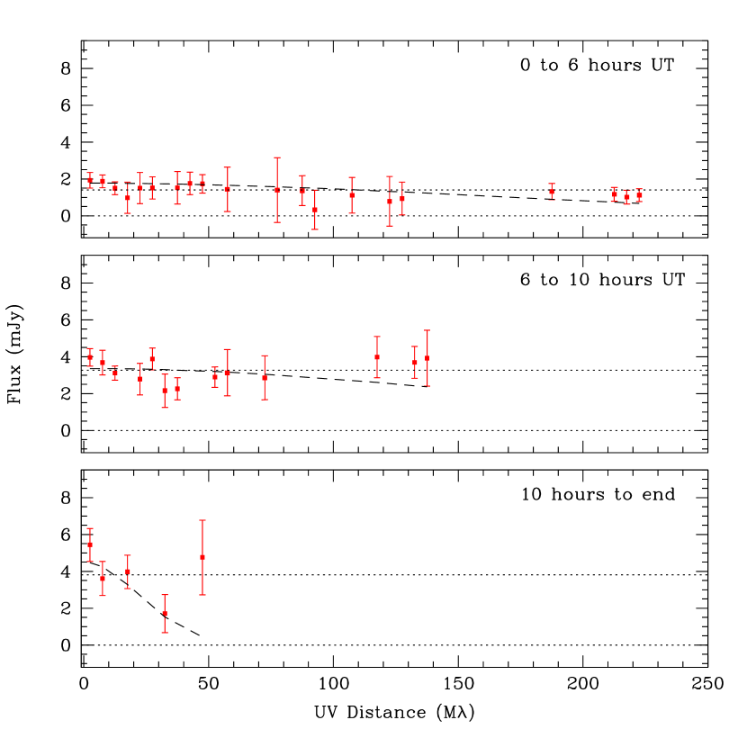
Figure 4: Correlated flux vs uv distance. The panels show (top to bottom) the visibility amplitude for the time periods 0 to 6 hours, 6 hours to 10 hours and 10 hours to the end of the observation. These time segments correspond to the three stages of flaring behaviour seen in Figure 3. The dotted straight lines mark the weighted data average. Dashed lines show the narrowest possible gaussian fitting the data. See the discussion in the text for details of the fits.

Plots of correlated flux against baseline distance for baselines including the VLA are shown in Figures 4 and 5. These plots were produced in the following way. For each baseline the complex phase-referenced visibility data were first averaged coherently in time over 25 - 30 minutes (the length of the scan groups shown in Figure 3), and then coherently averaged over the two IF channels, eight frequency channels and the RR and LL polarizations. From the scatter of the data over time error bars were assigned. These were propagated through subsequent averaging steps to determine the final error bars. On many baselines the phase versus time variations could be detected within the scans and be seen to be much less than a radian. Based on this and on the fact that the total flux in our VLBI map is comparable to the peak flux, we do not believe this averaging produced any significant loss of amplitude due to coherence losses over the averaging time chosen. At this point all baseline visibilities had signal to noise ratio significantly greater than unity. Finally the baseline amplitudes within annular shells in the uv plane were incoherently averaged and the results plotted as a function of baseline length. Because the signal to noise ratio of the original baseline averages were all greater than one the effect of noise-bias on the incoherently averaged amplitudes shown in Figure 4 is small. Given this, symmetric error bars are plotted.

The source is detected during the first interval from 0 to 6 hours with a flux around 1.4 mJy over the short baselines and is more clearly detected at the longest, but much more sensitive, Effelsberg baselines. The steady brightening in the following two periods can be clearly seen. It is unfortunate that Effelsberg baselines were only available for the first four hours of the experiment, so any information associated with the structure of the flaring source on such small scales is unavailable ($\sim 10$R_⊙).

We show in each plot a line marking the weighted average of the data points, which corresponds to a point-source model. In all cases the straight line is an acceptable fit to the data ($\chi^{2}=0.42$ for 0-6 hours, $\chi^{2}=0.75$ for 6-10 hours and $\chi^{2}=1.6$ for 10-11 hours). However, we wish to determine a meaningful upper limit for the source size. We have done this by fitting the narrowest possible Gaussian (representing the largest possible source) with the same $\chi^{2}$ as the straight line. The Gaussian amplitude is left as a free parameter. In the second data segment (6 to 10 hours UT), the $\chi^{2}$ for the fit never converged to the straight line. We therefore show the narrowest fit which attained $\chi^{2}=1$. The values of HWHM for the fitted Gaussians and HWHM of the corresponding Gaussian source on the sky are given in Table 3.

In Figure 5 the right- and left-handed polarizations are shown separately for the time segments 6-10 hours and 10 hours to the end of the experiment. The Stokes LL data from Mauna Kea were flagged during the last part of the experiment, and for this reason the longest baseline is missing from the final LL plot (lower right-hand panel). The enhanced brightening at RR can be clearly seen. Also clearly seen is the fact that LL does not brighten at all during the second flare, whereas RR does. This is consistent with the lightcurve shown in Figure 3. We have determined upper limits to the source sizes for the separate RR and LL data in the same way as described above. These are also listed in Table 3.

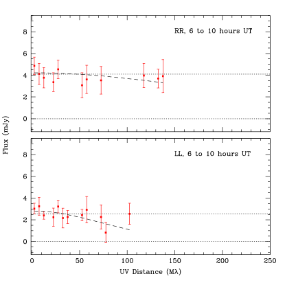
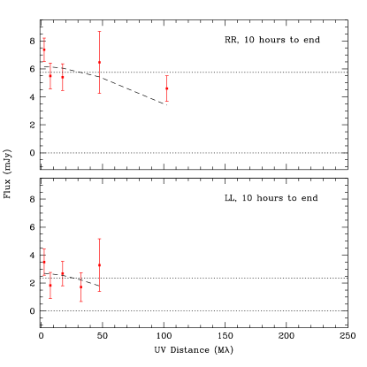
Figure 5: Correlated polarized flux vs uv distance for the periods of the two flares, separated in RR and LL. For the description of the plots see Figure 4. The LL data for Mauna Kea after UT=10 hours, which forms the longest baselines at this time, was flagged as unreliable and so the long baseline point is missing in the lower right-hand panel.

4 Discussion

4.1 T Tau N

T Tau N is not resolved in the VLA map, which has a maximum baseline separation of $\sim$300 k$\lambda$, but is resolved-out by the VLBI. This constrains its size to be between roughly 20 mas and 300 mas. A 20 mas source corresponds to 2.8 AU at 140 pc, which is large enough to rule out a coronal or magnetospheric origin for the flux and instead point to a wind source. The lack of variability or polarization tends to reinforce this conclusion.

Using the equations given in Panagia & Felli (1975) for a fully ionized, isotropic, optically thick envelope with $n_{e}\propto r^{-2}$, and assuming the outflow velocity to be 240kms^-1 (after Skinner & Brown) we can estimate the mass loss rate to be $5\times 10^{-8}$ M_⊙yr^-1 for a source of size 20 mas or $8\times 10^{-8}$ M_⊙yr^-1 for a source of size 500 mas. These values are up to a factor of 2 higher than those estimated by Skinner & Brown (1994). Because we have constraints both on the source size and the flux, we can also estimate the electron temperature. For a source of size 20 mas, the electron temperature would be around $2\times 10^{4}$ K. For a source of around 80 mas, the implied electron temperature would fall to around 5000K. Sizes larger than this are therefore unlikely. The corresponding brightness temperatures can be calculated from

$$T_{b}=\frac{c^{2}S_{L,R}}{\nu^{2}k\Delta\Omega}=4.43\times 10^{8}\nu_{9}^{-2}F_{mJy}r_{mas}^{-2},$$ (1)

where $S_{L,R}$ is the Planck function, $\nu_{9}$ is the frequency in GHz, $F$ is the total source flux (including both polarizations) and $r$ is the source size (HWHM). For an 80 mas source, $T_{b}=7055\leavevmode\nobreak\ K$. For 20 mas, it is $1.1\times 10^{5}$ K. These values are consistent with the interpretation of thermal wind emission.

4.2 T Tau Sa

No source could be seen corresponding to T Tau Sa. The RMS noise in the region of the map where Sa was expected to lie was approximately 0.1 mJy. A comparison of the flux at the peak of the VLA map with the flux of the compact source identified as Sb reveals that around 4.5 mJy can be attributed to a source which appears compact to the VLA ($\theta<500$ mas), but is apparently resolved-out by the VLBI array ($\theta>50$ mas). Only a small fraction of this flux will be contamination from T Tau N, some may correspond to the extended structure seen by Ray et al., and some may be due to an extended source associated with T Tau Sa.

Table 3: Upper limits on source sizes at various times for different polarizations. The size is given as the half width half maximum of the fitted Gaussian, $H$, the corresponding HWHM on the sky in milliarcseconds and the physical source size for a distance of 140pc (Elias, 1978) in solar radii.

	Polarization
	I			RR			LL
Time	H (M$\lambda$)	r (mas)	(R⊙)	H (M$\lambda$)	r (mas)	(R⊙)	H (M$\lambda$)	r (mas)	(R⊙)
0 - 6	189	0.48	14.4	172	0.53	15.9	192	0.47	14.3
6 - 10	193∗	0.47	14.2	231	0.39	11.9	87	1.05	31.5
10 - 12	26	3.5	105.4	111	0.81	24.7	62	1.47	44.2

4.3 T Tau Sb

The flux of T Tau S comprises a steady, extended component of about 4.5 mJy, which seems to be connected either to the circumbinary environment or to T Tau Sa, together with a compact, varying component which can be identified as T Tau Sb. This has a quiescent level of 1.4 mJy rising up to steady levels of 3.8mJy, with some spikes up to around 7 mJy. The extra flux in the two brightenings in the VLA lightcurve at UT=7 hours and UT=10hours is consistent with the extra flux seen in the VLBI data segments. This shows that the compact VLBI object can be confidently identified as the source of the rapidly varying flux. We found in the VLBI map no sign of the extended polarized structures reported by Ray et al. (1997) tracing the outflow, or of any structure to the northeast which could correspond to that seen by White and coworkers (White, 2000). The beam size in the Ray et al. maps was of the order of 150 mas, the individual left- and right-hand polarized blobs appear pointlike at this resolution in their maps, and the offset between them was around 200 mas. The structure seen by Ray et al. would not be expected to be resolved in low resolution VLA map, but could nevertheless be resolved out in the VLBI data. The flux of 2.1 mJy reported by Ray et al. is below the flux level of around 3 mJy which we believe is resolved out by the VLBI (see Table 2). A source size of around 100 mas corresponds to a scale around 1M$\lambda$ in the visibility functions. The shortest VLBI baseline is VLA-Pie Town (PT), with a uv distance of around 1M$\lambda$. We see no evidence of resolution within the set of VLA-PT scans, or between these and the next shortest baseline. Nevertheless, our visibility amplitudes are poorly sampled on these scales, and we cannot rule out that there is structure there which is missed. It should of course be borne in mind that these sources are intrinsically variable. Furthermore, in the case of blobs of outflowing material, significant motion may well have occurred on time scales of years between the observations.

The circular polarization is an indicator of the presence of magnetic fields. The short timescale variability, from hours down to seconds, together with MK brightness temperatures, points to a gyrosynchrotron emission mechanism. The 100% right-hand polarized emission which is seen in the spike at 7 hours UT and again more prominently at 11 hours UT probably arises from a coherent emission mechanism. This is discussed further below.

The initial luminosity was around $1.3\times 10^{17}$ erg s^-1 Hz^-1. The extra flux appearing after UT=7 hours has a luminosity of $4.4\times 10^{16}$ erg s^-1 Hz^-1. The luminosity of the extra flux appearing after UT=11 hours was $1.8\times 10^{16}$ erg s^-1 Hz^-1. Both the steady luminosity and the extra flux appearing during the variations have similar values to those observed in typical RS CVn systems, whose flux is also believed to arise in large-scale powerful magnetic fields (e.g. Benz & Güdel, 1994).

The polarization flip which was observed with the first flux increase at UT=7 hours is similar to that seen by Skinner & Brown (1994). They attributed this to a change in the relative optical depth of the $o$- and $x$-modes during the brighter phase, after a model for RS CVn systems developed by Morris, Mutel & Su (1990). Since these modes correspond (under normal conditions) to different observed polarizations, such changes can lead to the observed polarization flip. Another possible explanation would be a change in the sense of the dominant magnetic field along the line of sight, perhaps caused by stellar rotation, or the addition of new highly-polarized emission.

The size of the compact source is constrained from the VLBI data to be less than 0.48 mas. At a distance of 140 pc this corresponds to a scale of 14.5 R_⊙. This length scale is not much larger than the expected size of a T Tauri magnetosphere. We can also estimate the size of the varying region from the timescale of the flux variations. The most rapid variations take place on timescales down to our fundamental integration time of 10 s. This indicates a source of length scale at most $c\times dt=3\times 10^{9}$ m, or 4.3 R_⊙. This yields a lower limit to the brightness temperature of around $2\times 10^{9}$ K for the region involved in the rapidly varying emission in each case. Whilst this is still consistent with gyrosynchrotron emission from non-thermal electrons, the 100% right-hand polarization of the extra flux seen after the second flux increase is not. A coherent emission mechanism must be invoked to produce this strong polarization.

The most likely coherent emission process is an electron cyclotron maser, arising from mildly relativistic electrons trapped in magnetic flux tubes, where a loss-cone distribution may develop. This emission would occur at the fundamental or a low harmonic of the gyrofrequency

$$\nu_{c}=\frac{eB}{2\pi m_{e}c}\approx 2.8\times 10^{6}B.$$ (2)

8.4GHz emission at the fundamental or first harmonic therefore implies a magnetic field strength $B\sim 1.5-3$kG. Although the emission from an individual maser pulse would typically have a frequency range of about 1%, the emission arises from a range of locations in the flux tube and hence a range of magnetic field strengths, which gives rise to a much broader spectrum.

The main alternative to this would be a plasma maser, with the emitting frequency being the fundamental or first harmonic of the plasma frequency

$$\nu_{p}=\left(\frac{n_{e}e^{2}}{\pi m_{e}}\right)^{\frac{1}{2}}\approx 9000n_{e}^{0.5}$$ (3)

or at the hybrid frequency $(\nu_{p}^{2}+\nu_{c}^{2})^{1/2}$ with $\nu_{p}>\nu_{c}$. This would imply $n_{e}\sim 10^{12}$cm^-3.

For an accreting T Tauri star, a possible hypothetical emitting region is a magnetically confined accretion funnel, which would provide a region with magnetic field, high density and high density gradients at the stream edge. For a typical T Tauri accretion rate of $10^{-7}-10^{-8}$M_⊙ yr^-1 assuming the stream footpoint covers 10% of the stellar surface and that the inflow velocity is 150kms^-1, the density of material in the inner stream can be expected to reach perhaps $7\times 10^{-11}$g cm^-3, or about $5\times 10^{13}$cm^-3, consistent with the required density estimated above. We note that X-ray observations of He-like triplets in the X-ray spectrum of the nearby accreting T Tauri star TW Hya also indicates densities of the order $10^{13}$cm^-1 in the line-forming region, (Kastner et al., 2002).

Since for free-free absorption the optical depth for plasma emission is $\tau\propto\nu^{2}$, such emission would be expected to be heavily absorbed. A density scale length of less than 100 km would be necessary for this process to account for the emission, assuming second harmonic (Benz, 2002, eq. 11.2.5). The source size would have to be the same scale or even smaller and a brightness temperature in excess of $10^{18}$K is required. This exceeds solar radio bursts by three orders of magnitude.

Lower limits to the brightness temperature at various times were estimated for the upper limit source size and are shown in Table 4. A second estimate was also made assuming the upper limit source size is a constant 0.48 mas, the maximum size for the quiescent source between the beginning of the observation and UT=6 hours. This constraint was preferred because it is the most reliable, including the long Effelsberg-VLA baselines, and it is considered unlikely that the source would increase in size. The larger upper limits for the subsequent data segments are clearly driven by the lack of the long VLA-Effelsberg baselines. The brightness temperatures are at the high end of the range typically seen in solar gyrosynchrotron flares ($10^{7}$ – $10^{8}$K).

Table 4: Brightness temperature lower limits for T Tau Sb. The fourth column contains brightness temperatures for the source size constraint listed in column 2. The fifth column shows values calculated for an assumed constant source size upper limit of 0.48 mas.

Time	r (mas)	Flux (mJy)	T${}_{b}^{1}$ (K)	T${}_{b}^{2}$ (K)
0 - 6	0.48	1.4	3.8$\times 10^{7}$	3.8$\times 10^{7}$
6 - 10	0.47	3.3	9.4$\times 10^{7}$	9.4$\times 10^{7}$
10 - 12	3.5	3.8	1.9$\times 10^{6}$	1.0$\times 10^{8}$

The VLBI constraints show that the gyrosynchrotron compact source is contained within a volume approximately 15 R_⊙ in radius. The strength of the magnetic field implicated in the maser strongly suggests an origin for this emission close to the stellar surface, in the region with strongest magnetic field strength. The value of 1.5-3kG is consistent with values found in sunspots. It is also broadly consistent with values found using other techniques for T Tauri stars. For example, Guenther et al. (1999) used a technique based on Zeeman broadening of infrared Fe lines and determined magnetic field strengths of 2.35 kG in the case of T Tauri N, and 1.1 kG for LkCa 15, a weak-lined T Tauri star. Marginal detections of kilogauss strength fields were made for two other stars, one classical (accreting) and one weak-lined (non-accreting). It should be noted that these fields represent the average field over the entire stellar surface, so that local field strengths could be much higher. Basri et al. (1992) also used a similar technique to make one detection and establish one upper limit on two weak-lined T Tauri stars. Johns-Krull et al. (1999a) used spectropolarimetry of the accreting T Tauri star BP Tau to detect a field of 2.4kG associated with the He I $\lambda 5876$ line, which is believed to form in a high temperature accretion shock. A null result from photospheric lines indicates that this strong field is not globally present and points to magnetically funnelled accretion in this source.

Our observations point to strong magnetic fields and reconnection in the immediate environment ($<15$R_⊙) of T Tau Sb. It is tempting to speculate that this magnetic region is the actual field linking the star with a disk, which would then be responsible also for funnelling accreting material onto the star, and that the reconnection is driven by field lines being twisted by the differential rotation of star and inner disk. Could this be the case? The persistent polarized emission suggests that the emission arises in regions with magnetic fields that are large scale and persistent on timescales of $\sim$12 hours. We can impose a minimum scale size on the emitting region, if we require that the emission before UT=6 hours is gyrosynchrotron emission from non-thermal electrons, and impose a limit on the maximum allowable brightness temperature. The gyrosynchrotron brightness temperature is limited by the mean energy of the radiating particles. For a maximum allowed T_b of $10^{9}$ K the minimum source radius would be approximately 3 R_⊙. If we allow T_b to be as high as $10^{10}$ K, requiring electrons in the MeV range, the minimum source radius would be about 1 R_⊙. For the emission between UT=7 hours and UT=10 hours, the minimum source size is 4 R_⊙ for T_b=10⁹ K or 1.5 R_⊙ for T_b=10¹⁰ K. The expected size of a T Tauri magnetosphere can be roughly estimated from the assumed field strength and accretion rate, e.g. from Clarke et al. (1995)

$$R_{m}=\left(\frac{2B_{*}^{2}R_{*}^{6}}{(GM_{*})^{1/2}\dot{M}}\right)^{2/7}.$$ (4)

Taking $B_{*}$=1.5 kG, as estimated above, $R_{*}=1.5R_{\odot}$, $M_{*}=0.25M_{\odot}$, typical for a pre-main sequence M-dwarf, and $\dot{M}=10^{-7}\leavevmode\nobreak\ M_{\odot}$ yr^-1, which is at the high end of the range of typical classical T Tauri accretion rates, we would expect $R_{m}\sim 15\leavevmode\nobreak\ R_{\odot}$. Thus the magnetic field of T Tau Sb has a scale size consistent with the expected size of a classical T Tauri magnetosphere.

5 Conclusion

Our 8.4GHz observation of T Tau suggests three types of emission: Thermal emission from wind sources that are extended, a slowly varying gyrosynchrotron source and a highly-polarized maser source.

In the high resolution VLBI data, only one pointlike source is observed. We identify this as the southern component T Tau Sb. Intercontinental VLA-Effelsberg baselines in the early part of the experiment allow us to constrain the size of this source to be less than 14.5 R_⊙ in radius. Circular polarization indicates the presence of magnetic fields in the source region. Short timescale variability is observed, in the form of two distinct step-like flux increases, each followed by steady increased flux. During the first of these, the observed polarization changed from left- to right-handed. The second seems to have added only right-hand polarized flux. We argue that this strongly indicates coherent emission, most probably an electron-cyclotron maser. Based on this interpretation the magnetic field strength in the maser emitting region can be estimated to be in the kilogauss range.

By arguing that the quiescent emission in the first 6 hours represents gyrosynchrotron emission from non-thermal electrons and requiring the brightness temperature for this emission to lie below sensible limits, we argue that the emitting magnetic region must be at least 1 R_⊙ in size, and probably larger. The gyrosynchrotron emitting regions have sizes of the same order as those expected for an accreting magnetosphere.

At low resolution the system is resolved into the two components, N and S. T Tau N is consistent with a point source in our VLA maps. T Tau S shows evidence of resolved flux, indicating that there is either diffuse emission, or additional components in the system, or both. The non-detection of T Tau N in the high resolution data indicates that this is a wind source. The non-detection of T Tau Sa may indicate that this source is below our detection limit, although it is possible that it is resolved out by our shortest VLBI baseline.

- (1) Basri G., Marcy G.W. & Valenti J.A., 1992, ApJ 390, 622
- (2) Benz A.O., Plasma Astrophysics, second edition, Astrophysics and Space Science Library, Vol. 279, Kluwer Academic Publishers, Dordrecht, 2002.
- (3) Benz A.O. & Güdel M., 1994, A&A 285, 621
- (4) Clarke C.J., Armitage P.J, Smith K.W. & Pringle J.E., 1995, MNRAS 273, 639
- (5) Duchêne G., Ghez A.M. & McCabe C., 2002, ApJ 568, 771
- (6) Dyck H.M., Simon T. & Zuckerman B., 1982, ApJ 255, 103
- (7) Elias J.H., 1978, ApJ 224, 857
- (8) Ghez A. M., Neugebauer G., Gorham P. W., et al., 1991, AJ 102, 2066.
- (9) Guenther E.W., Lehmann H., Emerson, J.P. & Staude J., 1999, A&A 341, 768
- (10) Hayashi M.R., Shibata K. & Matsumoto R., 1996, ApJ 468, L37
- (11) Johns-Krull C.M., Valenti J.A., Hatzes A.P. & Kanaan A., 1999a, ApJ 510, L41.
- (12) Johns-Krull C.M., Valenti J.A. & Koresko C., 1999b, ApJ 516, 900
- (13) Johnston K.J., Gaume R.A., Fey A.L., de Vegt C. & Claussen M.J., 2003, ApJ 125, 858
- (14) Kastner J.H., Huenemoerder D.P., Schulz N.S., Canizares C.R., & Weintraub D.A., 2002, ApJ 567, 434
- (15) Köhler R., Kasper M. & Herbst T., 2000, In Birth and evolution of Binary stars poster proceedings of IAU Symp. 200, Reipurth & Zinnecker (eds) p63.
- (16) Koresko C.D., 2000, ApJ 531, L147
- (17) van Langevelde H.J, van Dishoeck E.F., van der Werf P.P. & Blake G.A. 1994, A&A 287, L25
- (18) Momose M., Ohashi N., Kawabe R., Hayashi M. & Nakano T., 1996, ApJ 470, 1001
- (19) Montmerle T., Grosso N., Tsuboi Y. & Koyama K., 2000, ApJ 532, 1097
- (20) Morris D.H., Mutel R.L. & Su B., 1990, ApJ 362, 299
- (21) Philips R.B., Lonsdale C.J. & Feigelson E.D., 1993, ApJ 403, L43
- (22) Ray, T.P., Muxlow T.W.B., Axon D.J., et al., 1997, Nature 385, 415
- (23) Roddier, F., Roddier C., Brandner W., Charrissoux D., Véran J.-P. & Courbin F., 2000, In IAU Symp. 200 Birth and Evolution of Binary Stars, poster proceedings, Reipurth & Zinnecker (eds), p60.
- (24) Skinner, S.L. & Brown A., 1994, AJ 107, 1461
- (25) White, S.M. 2000, In Radio Interferometry: The Saga and the Science, ed. DG Finley, W Miller Goss, NRAO workshop no 27, pp. 86–111. Associated Universities, Inc.
- (26) Wood K., Smith D., Whitney B., et al., 2001, ApJ 561, 299