Search for the Optical Counterpart of the Vela Pulsar X-ray Nebula

Abstract

Observations of the Vela pulsar region with the Chandra X-ray observatory have revealed the fine structure of its synchrotron pulsar-wind nebula (PWN), which showed an overall similarity with the Crab PWN. However, contrary to the Crab, no firm detection of the Vela PWN in optical has been reported yet. To search for the optical counterpart of the X-ray PWN, we analyzed deep optical observations performed with different telescopes. We compared the optical images with those obtained with the Chandra ACIS to search for extended emission patterns which could be identified as counterparts of the X-ray nebula elements. Although some features are seen in the optical images, we find no correlation with the X-ray structure. Thus, we conclude that the diffuse optical emission is more likely associated with filaments in the host Vela SNR. The derived upper limits on the optical flux from the PWN are compatibile, within the uncertainties, with the values expected on the basis of the extrapolations of the X-ray data.

1 Introduction

A compact ($\sim 4^{\prime}$) X-ray nebula around the Vela pulsar was first detected in soft X-rays by Harnden et al. (1985) with the Einstein High Resolution Imager (HRI). These authors suggested that it is a pulsar-wind nebula (PWN) powered by relativistic particles ejected by the pulsar. The soft X-ray emission from the Vela X-ray nebula was further studied with ROSAT (Ögelman, Finley & Zimmerman 1993; Markwardt & Ögelman 1998, and references therein). Based on its “kidney-bean” shape, Markwardt & Ögelman (1998) proposed an interpretation in terms of a bow-shock produced by the supersonic motion of the pulsar through the ambient medium.

The Vela pulsar and its PWN have been later observed with both the High Resolution Camera (HRC) and the Advanced CCD Imaging Spectrometer (ACIS) on board the Chandra X-ray observatory (Pavlov et al. 2000, 2001a,b, 2003; Helfand, Gotthelf, & Halpern 2001; Kargaltsev et al. 2002). Thanks to the excellent angular resolution of Chandra, the morphology of the PWN was resolved in a complex structure resembling that of the Crab PWN. Such a structure cannot be explained by a simple bow-shock model. The brighter part of the PWN, with a size of about $2^{\prime}$, shows an approximately axisymmetric structure, with two arcs, a jet, and a counter-jet, embedded into an extended diffuse emission. The axis of symmetry, which can be associated with the pulsar rotational axis (Pavlov et al. 2000), coincides, within the errors, with the direction of the pulsar’s proper motion (P.A. = 301°— e.g., Caraveo et al. 2001a).

The overall spectrum of the PWN can be described by a power law with an average spectral (energy) index $\alpha\approx 0.5$ (see Kargaltsev et al.  2002 for details), which can be interpreted as synchrotron emission of relativistic electrons and/or positrons. The same electron distributions should emit optical and radio synchrotron radiation, provided that the electron power-law spectrum extends down to sufficiently low energies, $\lesssim 300\nu_{14}^{1/2}B_{-4}^{-1/2}$ GeV (where $\nu=10^{14}\nu_{14}$ Hz is the radiation frequency, and $B=10^{-4}B_{-4}$ G is the magnetic field), and synchrotron self-absorption plays no role.

Indeed, highly polarized ($\approx 60$% at 5.2 GHz) extended radio emission has been recently detected around the Vela pulsar (Lewis et al. 2002; Dodson et al. 2003), covering a region $\sim\!4$ times larger than the X-ray PWN, as observed in the case of the Crab. Most of the diffuse radio emission comes from two lobes (see Figs. 2–4 in Dodson et al. 2003) — the southeast lobe of an area of 18 arcmin² ($F_{\nu}=760\pm 100$ mJy at 5.2 GHz) and a brighter northeast lobe of an area of 5.3 arcmin² ($F_{\nu}=290\pm 50$ mJy at 5.2 GHz). Search for radio emission from the X-ray-bright compact nebula was hampered by the brightness of the pulsar. Although some emission was detected (e.g, about 30 mJy at $\nu=2.4$ GHz, in a 0.73 arcmin² area around the pulsar), it can well be an unsubtracted pulsar contribution and should be considered as an upper limit on the compact PWN emission.

One could expect to see optical nebula around the Vela pulsar. Indeed, optical PWNe have been observed in several other young pulsars. The most famous example is the Crab PWN (see, e.g., Hester et al. 2002, and references therein) which exhibits a complex structure featuring bright knots and sharp arc-like features dubbed “wisps” (Scargle 1969) located at the inner boundary of the X-ray torus and probably associated with a termination shock in the pulsar wind (e.g., Hester et al.  1995; Kennel & Coroniti 1984). Also, the comparison between the Hubble Space Telescope (HST) and Chandra observations of the LMC pulsar B0540–69 has clearly shown the presence of an optical PWN which follows exactly the morphology of the X-ray PWN (Caraveo et al. 2001b, 2003).

Contrary to the Crab and PSR B0540–69, searches for the Vela PWN in optical have been inconclusive so far. The only marginal detection of an optical PWN was reported by Ögelman et al. (1989), who observed the Vela pulsar field in the $V$ and $B$ bands with the ESO 2.2 m telescope. These authors found evidence for optical diffuse emission (typical size $\sim 2^{\prime}$), with an average surface brightness of about 26 mag arcsec^-2. However, the presence of bright filaments from the host SNR, as well as of several bright stars in the field, made it difficult to assess the reality of the putative optical nebula.

The increase in sensitivity and angular resolution provided by the HST prompted us to carry out a new optical investigation of the Vela pulsar region. In the following, we discuss spatial correlations between Chandra ACIS images (Pavlov et al. 2001b; Pavlov et al. 2003) and the optical ones collected by both the HST WFPC2 (Mignani and Caraveo 2001; Caraveo et al. 2001a) and ESO NTT (Nasuti et al. 1997) and VLT.

2 X-ray and optical observations

2.1 Chandra observations

The multiple observations of the Vela PWN with the Chandra  ACIS are described by Pavlov et al. (2003). In all the observations the PWN was imaged on the same back-illuminated chip S3, more sensitive to soft X-rays. Although the individual images show some variability of the PWN elements, the overall PWN morphology remains stable. To obtain a very deep X-ray image to be compared with the optical ones, we stacked seven consecutive individual images, collected from 2001 November 25 through 2002 April 3 for a total exposure time of 141 ks, and adaptively smoothed the combined image. The accuracy of the image co-alignment was about 0$\farcs$7. The smoothed X-ray image of the PWN, in the energy band 1–8 keV, is shown in Figure 1. The logarithmic brightness scale was chosen to increase the dynamic range. The jet and the counter-jet, northwest and southeast of the pulsar, respectively, and two arc-like structures (inner and outer arcs) are the dominant features of the bright inner nebula (upper panel). The inner nebula is surrounded by a bean-shaped region of diffuse emission (outer nebula), $\sim 2^{\prime}\times 2^{\prime}$ in size (lower panel). An elongated region of fainter extended emission southwest of the bright inner PWN is seen up to the edge of the ACIS image ($\sim 4^{\prime}$ from the pulsar). A $100^{\prime\prime}$-long outer jet is seen northwest of the inner PWN. The spectrum of the bright inner PWN, within a $45^{\prime\prime}$ radius around the pulsar, can be fitted by a single power-law model with a spectral index $\alpha=0.47\pm 0.02$ and unabsorbed flux of $9.1\pm 0.7\times 10^{-11}$ ergs s^-1 cm^-2, in the 0.1–10 keV range (Kargaltsev et al.  2002). The unabsorbed surface brightnesses for the outer and inner arcs are about $6\times 10^{-14}$ and $3\times 10^{-14}$ ergs s^-1 cm^-2 arcsec^-2, while the spectral indices $\alpha$ are about 0.4 and 0.3, respectively.

2.2 Optical wide-band imaging

Optical observations of the Vela pulsar field were collected at different epochs using different telescopes, instrumentation, observational set-ups, and filters. In addition to the recent high-resolution imaging data obtained with the HST, our data set includes archived ground-based images obtained from ESO with the NTT and the VLT. Table 1 gives a detailed summary of the available observations.

2.2.1 HST

HST observations of the Vela pulsar field were collected between 1997 June and 2000 March with the WFPC2. Several images have been taken through the filters $675W$ ($\lambda=6717$Å; $\Delta\lambda=1536$Å), $814W$ ($\lambda=7995$Å; $\Delta\lambda=1292$Å) and $555W$ ($\lambda=5500$Å; $\Delta\lambda=1200$Å) with exposure times ranging between 2000 s and 2600 s. These data were originally taken as part of two independent programs aimed at the study of the multicolor flux distribution of the pulsar (Mignani & Caraveo 2001) and at the measure of its parallactic displacement (Caraveo et al. 2001a). To achieve the maximum spatial resolution, in all the exposures the pulsar was located near the center of the Planetary Camera chip, with a pixel size of $0\farcs 045$ and a field of view of $35^{\prime\prime}\times 35^{\prime\prime}$. The standard HST pipeline was applied for the image reduction and for the photometric calibrations. Co-aligned exposures were finally combined to filter out cosmic ray hits (see Mignani & Caraveo 2001 and Caraveo et al. 2001a for a detailed description of the observations and data reduction).

For each observation, the IRAF/STSDAS task wmosaic was used to obtain a mosaic of the four WFPC2 images and correct for the instrumental geometric distortion of the cameras (Casertano & Wiggs 2001). To increase the signal-to-noise ratio, we combined all the available $555W$ filter images. Since the observations at different epochs were performed with different telescope pointings and roll angles, to superpose the frames we had to follow the procedure successfully applied in previous astrometric works, using a common reference frame defined by a grid of reference stars’ coordinates (see Caraveo et al.  2001a and references therein for further details). Images were registered within $\approx 0.1$ WFC pixels ($\approx$ 10 mas), an accuracy adequate to achieve the goals of the present investigation, co-aligned and stacked.

2.2.2 NTT

The Vela pulsar field was observed with the NTT at the La Silla observatory in January 1995 (Nasuti et al.  1997). To achieve the highest sensitivity both at longer and shorter wavelengths, the EMMI camera was used in both its Red (EMMI-R) and Blue (EMMI-B) arm modes. The camera is a TEK $2048\times 2048$ pixels CCD with a pixel size of 0$\farcs$27 (field of view $9\farcm 2\times 8\farcm 6$ ) and 0$\farcs$37 (field of view $6\farcm 2\times 6\farcm 2$) in the EMMI-R and EMMI-B configuration modes, respectively. Images were collected in the Johnson’s $U$ ($\lambda=3542$Å; $\Delta\lambda=542$Å), $B$ ($\lambda=4223$Å; $\Delta\lambda=941$Å), $V$ ($\lambda=5426$Å; $\Delta\lambda=1044$Å), and $R$ ($\lambda=6410$Å; $\Delta\lambda=1540$Å) bands with exposure times between 15 and 40 minutes. Data reduction and photometric calibration were carried out as described in Nasuti et al. (1997).

2.2.3 VLT

Observations of the field were performed in April 1999 with the first Unit Telescope (Antu) of the ESO VLT located at the Paranal Observatory. Images were obtained using the FOcal Reducer and Spectrograph #1 (FORS1) instrument, a four-port $2048\times 2048$ CCD detector which can be used both as a high/low resolution spectrograph and an imaging camera. The instrument was operated in imaging mode with a $1\times 1$ binning and at its standard angular resolution of 0.2 arcsec/pixel, with a corresponding field of view of $6\farcm 8\times 6\farcm 8$. Two 300 s exposures were taken in the Bessel filters $R$ ($\lambda=6570$Å; $\Delta\lambda=1500$Å) and $I$ ($\lambda=7680$Å; $\Delta\lambda=1380$Å) under good seeing conditions $(\leq 1^{\prime\prime}$). The images have been retrieved from the ESO public archive and reduced following standard procedures for debiassing and flatfielding. Since no standard stars were observed, absolute flux calibration was performed using as a reference a set of secondary stars detected in the same passbands in the NTT images.

2.3 Narrow-band imaging

Three 20-min exposures of the Vela pulsar field were taken in H_α ($\lambda=6588.27$Å, $\Delta\lambda=74.31$Å) on 1999 April 4 with the Wide Field Imager (WFI) at the ESO/MPG 2.2 m telescope. The WFI is a wide field mosaic camera, composed of eight $2048\times 4096$ pixel CCDs, with a scale of $0.238$ arcsec/pixel, providing a field of view of $33\farcm 7\times 32\farcm 7$. To compensate for the loss of signal due to the interchip gaps (23$\farcs$8 and 14$\farcs$3 along right ascension and declination, respectively), the second and third exposures were taken with a relative offset of $30\arcsec$ in RA and Dec. The images were taken in fairly good seeing conditions with FWHM$\simeq 0\farcs 9$. Data reduction with the usual CCD processing steps of bias subtraction, flat-fielding and trimming of images, was performed with IRAF using the Mosaic CCD reduction package (MSCRED). Individual exposures have been finally coadded and cleaned of cosmic-ray hits using the DRIZZLE software (Hook & Fruchter 1997) and the final image has been corrected for the effects of fringing that affects the CCDs in the red part of the spectrum ($\gtrsim 6500$ Å).

2.4 Image superposition: X-ray versus optical

The direct comparison of images taken in different energy bands (e.g., optical and X-rays) can be achieved through accurate image superposition. Following the approach used by Caraveo et al. (2001b), we superimposed the X-ray Chandra image onto the optical ones with respect to the absolute ($\alpha$,$\delta$) reference frame, relying on the astrometric solution of each image. We used the combined Chandra ACIS image, where individual images were co-aligned with an accuracy of $0\farcs 7$ (Pavlov et al. 2003). The error of the absolute Chandra aspect solution is typically about $0\farcs 6$. Therefore, we adopt $1^{\prime\prime}$ as a reasonable estimate for the uncertainty of the absolute X-ray astrometry.

For the WFPC2 images, the default astrometric solution across the focal plane is derived from the coordinates of the two guide stars used to point the telescope, which are taken as a reference to compute the astrometric reference point and the telescope roll angle. The accuracy of the HST astrometry is limited by the intrinsic error on the absolute coordinates of the GSC1.1 (Guide Star Catalog) stars (Lasker et al. 1990) which are used for the telescope pointing. According to the current estimates, the mean uncertainty of the absolute positions quoted in the GSC1.1 is about 0$\farcs$8 per coordinate (Biretta et al. 2002). For this reason, we have recomputed a new astrometric solution for the WFPC2 images by using as a reference the positions of several stars from the USNO-A2.0 catalog (Monet 1998) identified in the field of view. The ASTROM software was used to compute the pixel-to-sky coordinates transformation. The rms of the astrometric fit was $\sim 0\farcs 08$, per coordinate.

The astrometric calibrations of the the ground-based optical images was computed as described above. The astrometric fits yielded rms values of $\sim 0\farcs 13$ and $\sim 0\farcs 22$ per coordinate for the VLT and NTT images, respectively. For the WFI image, the astrometry was computed separately for each of the eight CCD chips, yielding an average rms of $\sim 0\farcs 3$.

In all cases, the final uncertainty on our astrometric solutions was evaluated by accounting both for the rms of the astrometric fits and for the propagation of the error on the intrinsic absolute accuracy of the USNO-A2.0 coordinates, which is of the order of $0\farcs 2$–$0\farcs 3$.

The absolute frame registration between the optical and X-ray images turned out to be accurate within $\approx 1^{\prime\prime}$, i.e., compatible with the overall uncertainties of the absolute astrometry of each frame. Unfortunately, the strong pile-up of the Vela pulsar in the ACIS images hampered the use of the pulsar position for better co-alignment between the X-ray and optical images.

3 Results

3.1 Search for a compact optical nebula

As a first step, the central part of the X-ray PWN field (corresponding to the inner nebula and the outer nebula) was inspected to search for optical counterparts of the complex structures seen with Chandra. Our starting point was the combined WFPC2 $555W$ image, which is by far the deepest optical image of the Vela pulsar field. The final image is shown in Figure 2, where we superimposed the X-ray contour map obtained from the combined Chandra ACIS exposure of the region. Although a number of complicated patterns of diffuse emission are present in the $\approx 3^{\prime}\times 3^{\prime}$ field of view, no optical counterparts of the X-ray features seen in Figure 1 can be identified, nor any other structure symmetric with respect to the axis of symmetry of the X-ray PWN. We thus conclude that the PWN is undetected in the optical.

To compute the upper limit on the optical surface brightness of the PWN, an accurate mapping of the background is required. This is complicated by the presence of diffuse, non-uniform, emission patterns which show sharp surface brightness variations on angular scales as small as $\approx 5$ arcsec. For this reason, we evaluated the background level in $\approx 200$ cells of 1 arcsec² each, selected in a number of star-free regions across the whole image. Statistical errors on the number of counts per cell were of the order of 0.3%. The background level, $\approx 22.3$ ST magnitudes  arcsec^-2 on average, was found to vary typically by 4%–5% across the whole field, with a maximum variation of $\approx$ 7%.

For an extended source, the upper limits on the surface brightness scale with the detection area ${\cal A}$ as ${\cal A}^{-1/2}$. An optimally chosen area should be large enough to reduce the statistical errors due to the background fluctuations but it should be smaller than the scale of sharp background variations. According to our mapping of the background, a detection area of 10 arcsec² represents a resonable optimization.

For the area chosen, the measured background variations affect the upper limit on the flux of an extended source (at a 3 $\sigma$ level) by no more than $\approx$3%, corresponding to surface brightness variations below 0.1 magnitudes arcsec^-2.

While variations in the sky background across the image play a minor role, we found that the derived surface brightness upper limits are different in different regions of the image. This is mainly due to the non-uniform coverage of the field performed by the WFPC2. First, because of the intrinsic differences in the pixel size and in the physical characteristics of the CCDs, the PC and the WFC chips contribute differently to the instrumental background per unit area. In addition, since the five WFPC2 $555W$ observations listed in Table 1 were executed at different epochs and with different telescope roll angles, the exposure map varies across the field. For instance, the central region of the field, which is covered by the PC ($35^{\prime\prime}\times 35^{\prime\prime}$), reaches an integration time of 11 800 s, while the outer regions, covered by the three WFC chips, have integration times varying between 4 600 and 11 800 s.

Both effects clearly affect the evaluation of the surface brightness upper limits in different regions of the PWN, as they are covered differently by the four WFPC2 chips. As it is seen from Figure 2, some regions of the inner nebula (inner arc, jet, and counter-jet) fall entirely within the PC, while the outer arc is coincident with the inter-chip gaps and is covered partially by the PC and partially by the WFC chips. On the other hand, the outer nebula is entirely covered by the WFC chips.

Taking all these effects into account, we have computed the 3$\sigma$ upper limits on the optical surface brightness of both the inner nebula (inner arc, jet, counter-jet, outer arc) and the outer nebula. We note that although our upper limits have been computed for a detection area of 10 arcsec², they can be easily rescaled to any other area.

Using the HST pipeline photometric calibration, we computed an upper limit of 28.1 and 28.0–28.5 ST magnitudes arcsec^-2 for the inner nebula and for the outer nebula, respectively. As we mentioned before, because of the non-uniformity of the exposure map the upper limit for the outer nebula turned out to be slightly position-dependent. To correct these limits for the interstellar reddening, we use the extinction $A_{V}=0.2$, consistent with the hydrogen column density estimated from the X-ray observations of the Vela pulsar (Pavlov et al. 2001a). The corrected limits are 27.9 and 27.8–28.3 ST magnitudes arcsec^-2.

The same analysis was then repeated for the other available WFPC2 images ($675W$ and $814W$) as well as for the NTT ($UBVR$) and VLT ($VI$) ones (see Table 1) but no evidence for a compact optical nebula was found in either of these datasets. The computed upper limits are summarized in Table 2.

3.2 Search for an extended nebula

Since the emission from the PWN could, in principle, be visible at optical wavelenghts on larger angular scales with respect to the X-rays, as it has been observed in radio (see §1), we took advantage of the larger field of view provided by the NTT images to search for extended features up to distances of $\approx 3$ arcmin. In particular, we searched for diffuse optical emission at the position of the southwest extension of the X-ray nebula (see Fig. 1, lower panel). To go as deep as possible, we have combined all the available NTT $UBVR$ band images (Fig. 3, upper panel). The combined image shows many different enhancements in the background, with a rather complex spatial distribution. However, none of them can be firmly correlated with the known X-ray features. In addition, we note that almost all the diffuse emission patterns seen in the NTT $UBVR$ image can be also identified in the ESO/2.2m H_α (Fig. 3, lower panel). This suggests that they are most likely associated with the bright filaments of the Vela supernova remnant. We note that the computed NTT upper limits on the optical emission of the compact X-ray nebula can be applied also at larger distances from the pulsar. The maximum variation in surface brightness for source-free regions, due to the complicated distribution of diffuse emission, is found to be of order 7% even in the outer regions of the NTT field, which corresponds to $<0.1$ magnitudes arcsec^-2 variations of the upper limit across the field (see §3.1). We note that for the NTT images the measured upper limits in the $U$ and $B$ bands do not apply to the region $\approx$ 2.5 arcmin southwest of the pulsar position, close to the southwest edge of the extended X-ray nebula. The background in this region is unrecoverably polluted by the presence of a bright ($B\approx$9) B star that is not visible in the $V$ and $R$ band images because of the slightly narrower field of view.

4 Discussion

It is interesting to compare the measured upper limits on the optical brightness of the Vela PWN with the X-ray and radio observations. The observed X-ray spectra of the Vela PWN are described by a power law with spectral indices $\alpha\approx 0.3$–0.4 and $\alpha\approx 0.4$–0.5, for the arcs and the extended diffuse emission southwest of the pulsar, respectively (Kargaltsev et al. 2002). The X-ray and radio surface brightness spectra, together with the optical upper limits, are shown in Figure 4 for the outer arc (upper panel) and the diffuse emission southwest of the pulsar (lower panel). Since the inner PWN structures were not resolved in the radio (see §1), only radio upper limits are plotted in the upper panel. From the plot we see that both the optical and radio upper limits for the outer arc are within the uncertainty of the extrapolation of the X-ray spectrum towards lower frequencies.

In the case of the southwest diffuse emission, we note that the X-ray-to-radio extrapolation is well below the measured radio brightness values. This apparent inconsistency can be explained by the fact that the radio and X-ray brightnesses were measured in different areas (the X-ray image is substantially smaller than the radio image). Moreover, even within the smaller X-ray field-of-view, it is seen that the X-ray brightness of the southwest diffuse emission fades towards the region of maximum radio brightness (which is outside the X-ray field of view). Such behavior can be explained by radiative (synchrotron) and adiabatic cooling of the expanding cloud of relativistic electrons, which can result not only in the increase of the spectral index, but also in the shift of the lower-energy boundary of the power-law spectrum towards lower energies. Therefore, we can expect maximum optical brightness to be observed in between the regions of the X-ray and radio maximum brightnesses. Although the X-ray and radio spectra in the lower panel of Figure 4 cannot be directly compared with each other, a crude estimate of the expected optical brightness can be obtained by connecting the radio and X-ray points. This yields $\sim 3\times 10^{-32}$ erg cm^-2 s^-1 Hz^-1 arcsec^-2, i.e., about 3 magnitudes below our measured optical upper limit.

To summarize, we conclude that it is very likely that just a slightly deeper optical observation would allow one to detect the outer/inner arc (and other bright elements of the inner PWN), while much deeper optical observations are needed to detect the emission from the Vela PWN at large. However, owing to the presence of background/foreground emission from the SNR as well as numerous bright stars in the field, longer exposures would not help to detect the optical PWN — neither its X-ray-bright central part nor the radio-bright outskirts. To get rid of the contaminating emission, one should observe the field at UV wavelengths, where the radiation of most of the field stars would be much dimmer. Observing in polarized light appears even more promising. Since the synchrotron emission from the PWN should be highly polarized (as confirmed by the radio observations), polarimetry observations should allow one to minimize the contamination from field sources and provide a clean PWN image. Polarimetry observations of the Vela pulsar field have been recently obtained by Wagner and Seifert (2000) but they did not yield a conclusive result. Deeper, higher-resolution, observations are needed to unveal extended polarized emission from the PWN.

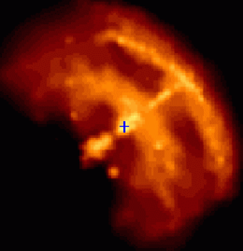
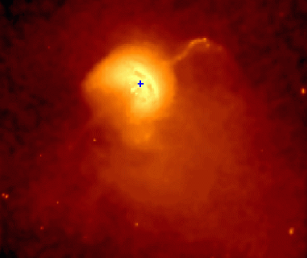
Figure 1: X-ray images of the Vela PWN, combined of seven individual Chandra ACIS images (see Pavlov et al. 2003). The upper panel ($1\farcm 60\times 1\farcm 35$) shows the bright inner PWN around the Vela pulsar (marked by the cross), with the outer and inner arcs, northwest inner jet, and southeast counter-jet. The brightness scale in the lower panel ($6\farcm 3\times 5\farcm 4$) was chosen so as to show the faint nebular structures — e.g., the northwest outer jet and the dim extended emission southwest of the bright inner PWN. North is up, East to the left.

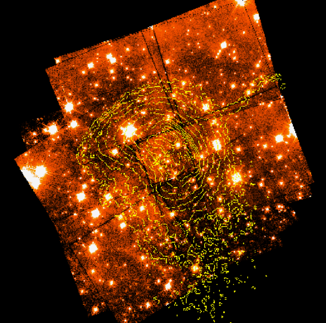
Figure 2: Image of the Vela pulsar field obtained by combining all the WFPC2 $555W$ observations listed in Table 1 (North to the top, East to the left). The gaps among different CCD chips are evident. The overall integration time on the central part, corresponding to the PC field of view, is 11 800 s (see text). The overlayed contours (logarithmic scale) correspond to the X-ray intensity maps obtained from the Chandra ACIS image of the field in the energy band 1–8 keV. The point source within the innermost X-ray contour is the optical counterpart of the Vela pulsar.

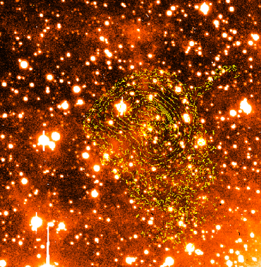
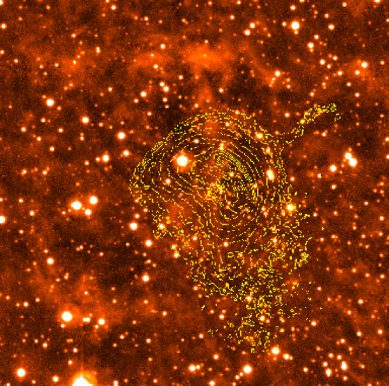
Figure 3: The upper panel shows the combined $UBVR$ image of the Vela pulsar field obtained from the NTT/EMMI observations listed in Table 1. The lower panel shows the ESO/2.2m H_α image. In both cases the image size is $\approx 4^{\prime}\times 4^{\prime}$ . North is up, East to the left. The X-ray contour plots of the Vela PWN derived from the seven ACIS observations (§2.1) are overlayed.

Figure 4: Spectra of surface brightness (in erg cm^-2 s^-1 Hz^-1 arcsec^-2) in X-rays (solid lines) and radio (points), together with the optical upper limits, for the inner/outer arc (upper panel) and diffuse emission southwest of the pulsar (lower panel). Expected brightness levels in optical, based on extrapolations of the X-ray and radio data, are shown with dashed lines.

Table 1: Available optical datasets for the Vela pulsar field.

Date	Telescope	Instr.	Filter	$\lambda~{}(\Delta\lambda)$	Exp.	Ref.
Jan 1995	NTT	EMMI-B	$U$	3542Å (542Å)	4800	(1)
Jan 1995	NTT	EMMI-B	$B$	4223Å (941Å)	1800	(1)
Jan 1995	NTT	EMMI-R	$V$	5426Å (1044Å)	1200	(1)
Jan 1995	NTT	EMMI-R	$R$	6410Å (1540Å)	900	(1)
June 1997	HST	WFPC2	$555W$	5500Å (1200Å)	2600	(2)
Jan 1998	HST	WFPC2	$555W$	-	2000	(2)
June 1999	HST	WFPC2	$555W$	-	2000	(2)
Jan 2000	HST	WFPC2	$555W$	-	2600	(2)
Jul 2000	HST	WFPC2	$555W$	-	2600	(2)
Mar 2000	HST	WFPC2	$675W$	6717Å (1536Å)	2600	(3)
Mar 2000	HST	WFPC2	$814W$	7995Å (1292Å)	2600	(3)
Apr 1999	VLT	FORS1	$R$	6750Å (1500Å)	300
Apr 1999	VLT	FORS1	$I$	7680Å (1380Å)	300
Apr 1999	2.2m	WFI	Hα	6588Å (74.3Å)	3600

Note. — First column lists the epoch of observation. Second and third columns show the telescope and the detector used for the observations, respectively. The filter names are listed in column four, with their pivot wavelengths and widths in column five. The total integration time per observation (in seconds) is given in column six. The last column provides the references: (1) Nasuti et al. 1997; (2) Caraveo et al. (2001a); (3) Mignani & Caraveo (2001).

Table 2: $3\sigma$ upper limits to the surface optical brightness of the X-ray PWN structures.

			Observed			Extinction-corrected
Telescope	Instrument	Filter	mag arcsec-2	Flux		mag arcsec-2	Flux
HST	WFPC2	$555W$	28.1	0.21		27.9	0.25
			28.5–28.0	0.15–0.23		28.3–27.8	0.18–0.28
	WFPC2	$675W$	27.5	0.55		27.3	0.66
			27.9	0.38		27.7	0.46
	WFPC2	$814W$	27.7	0.65		27.6	0.71
			28.1	0.45		28.0	0.49
NTT	EMMI-B	$U$	26.4	0.52		26.1	0.69
		$B$	27.4	0.47		27.1	0.62
	EMMI-R	$V$	27.1	0.53		26.9	0.64
		$R$	26.7	0.59		26.5	0.71
VLT	FORS1	$R$	27.0	0.45		26.8	0.54
		$I$	26.1	0.81		26.0	0.90

Note. — The upper limits are computed for an area of 10 arcsec². For the HST results, the first and second rows, for a given filter, are the upper limits measured in the PC and WFC chips, respectively. Due to the uneven exposure map of the combined WFPC2 $555W$ image (Fig. 2), slightly different upper limits are derived across the WFC field. For both the NTT and VLT, the upper limits apply to the overall X-ray nebula.

References

- (1)
- (2) Biretta, J.A. et al. 2002, WFPC2 Instrument Handbook, Version 7.0 (Baltimore, STScI)
- (3)
- (4) Caraveo, P. A., De Luca A., Mignani R. P., & Bignami, G. F. 2001a, ApJ, 561, 930
- (5)
- (6) Caraveo, P. A., Mignani, R. P., De Luca, A., Wagner, S., & Bignami, G. F. 2001b, in Proc. STScI Symp., A Decade of HST Science, eds. M. Livio, K. Noll, & M. Stiavelli (Baltimore: STScI), 105
- (7)
- (8) Caraveo, P. A., Mignani, R. P., De Luca, A., Wagner, S. & Bignami, G. F., 2003, in preparation
- (9)
- (10) Casertano, S. & Wiggs, M.S.2000, see WFPC2 Instrument Handbook v5.0, 2000, ed.STScI
- (11)
- (12) Dodson, R., Lewis, D., McConnel, D., Deshpande, A. A. 2003, MNRAS, submitted (astro-ph/0302373)
- (13)
- (14) Harnden, F. R., Grant, P. D., Seward, F. D., & Kahn, S. M., 1985, ApJ, 299, 828
- (15)
- (16) Helfand, D. J., Gotthelf, E. V., & Halpern, J. P. 2001, ApJ, 556, 380
- (17)
- (18) Hester, J. J., et al. 1995, ApJ, 448, 240
- (19)
- (20) Hester, J. J., Mori, K., Burrwos, D., et al. 2002, ApJ, 577, 49
- (21)
- (22) Hook, R. N. & Fruchter, A. S., 1997, in ASP Conf. Series, Vol. 125, Astronomical Data Analysis Software and Systems VI, ed. G. Hunt and H. E. Payne (San Francisco: ASP), 147
- (23)
- (24) Kargaltsev, O., Pavlov, G. G., Sanwal, D., & Garmire, G. P. 2002, in Neutron Stars in Supernova Remnants, ASP Conf. Ser., v.271, eds. P. O. Slane & B. M. Gaensler (ASP: San Francisco), 181
- (25)
- (26) Kennel, C. & Coroniti, F. 1984, ApJ, 283, 694
- (27)
- (28) Lewis, D., Dodson, R., McConnell, D., & Deshpande, A. 2002, in Neutron Stars in Supernova Remnants, ASP Conf. Ser., v.271, eds. P. O. Slane & B. M. Gaensler (ASP: San Francisco), 191
- (29)
- (30) Markwardt, C. B. & Ögelman, H. B. 1998, Mem. Soc. Astr. It., vol.69, p.927
- (31)
- (32) Mignani, R. P. & Caraveo, P. A., 2001, A&A, 376, 213
- (33)
- (34) Monet, D. G., et al. 1998, USNO-A20 (Washington: US Nav. Obs.)
- (35)
- (36) Nasuti, F. P., Mignani, R., Caraveo, P. A. & Bignami, G. F. 1997, A&A, 323, 839
- (37)
- (38) Ögelman, H. B, Koch-Miramond, L., & Aurieére, M. 1989, ApJ, 342, 83
- (39)
- (40) Ögelman, H., Finley, J. P., & Zimmerman, H. U. 1993, Nature, 361, 136
- (41)
- (42) Pavlov, G. G., Sanwal, D., Garmire, G. P., Zavlin, V. E., Burwitz, V., & Dodson, R. G. 2000, AAS Meeting 196, #37.04
- (43)
- (44) Pavlov, G. G., Zavlin, V. E., Sanwal, D., Burwitz, V., & Garmire, G. P. 2001a, ApJ, 552, 129
- (45)
- (46) Pavlov, G. G., Kargaltsev, O. Y., Sanwal, D., & Garmire, G. P.,2001b ApJ, 554, 189
- (47)
- (48) Pavlov, G. G., Teter, M. A., Kargaltsev, O., & Sanwal, D. 2003, ApJ, accepted
- (49)
- (50) Russell, J. L., Lasker, B. M., McLean, B. J., Sturch, C. R. & Jenkner, H., 1990, AJ99, 2059
- (51)
- (52) Scargle, J. D. 1969, ApJ, 156, 401
- (53)
- (54) Wagner, S. and Seifert S., 2000, in Proc. of the 177th IAU Colloquium Pulsar Astronomy - 2000 and Beyond, ASP Conference Series, Vol. 202, p. 315, M. Kramer, N. Wex, and N. Wielebinski Eds.
- (55)