Constraints on stellar convection from multi-colour photometry of $\delta$ Scuti stars

In $\delta$ Scuti star models, the calculated amplitude ratios and phase differences for multi-colour photometry exhibit a strong dependence on convection. These observables are tools for determination of the spherical harmonic degree, $\ell$, of the excited modes. The dependence on convection enters through the complex parameter $f$, which describes bolometric flux perturbation. We present a method of simultaneous determination of $f$ and harmonic degree $\ell$ from multi-colour data and apply it to three $\delta$ Scuti stars. The method indeed works. Determination of $\ell$ appears unique and the inferred $f$’s are sufficiently accurate to yield a useful constraint on models of stellar convection. Furthermore, the method helps to refine stellar parameters, especially if the identified mode is radial.

1 Introduction

The $\delta$ Scuti stars are pulsating variables located in the HR diagram at the intersection of the classical instability strip with the main sequence and somewhat above it. The observables of primary interest for asteroseismology are oscillation frequencies. However, information about amplitudes and phases of oscillations in various photometric passbands is also useful. So far the main application of multi-colour photometry of $\delta$ Scuti stars has been determination of $\ell$ degree of observed modes (see e.g. Balona & Evers 1999, Garrido 2000). This is an important application because knowledge of $\ell$ is an essential step for mode identification. The $\ell$ diagnostic makes use of diagrams in which the amplitude ratio determined in two passbands is plotted against the corresponding phase difference. The observational data are compared with ranges calculated for relevant stellar models and assumed $\ell$ values. The ranges reflect uncertainties in stellar parameters and physics. The inference is easy if the ranges do not overlap. This is largely true for $\beta$ Cephei stars, but not for $\delta$ Scuti stars. For the latter objects, a major uncertainty in the calculated ranges arises from lack of adequate theory of stellar convection.

Calculations of the amplitude ratios and phase differences make use of the complex parameter $f$, which gives the ratio of the radiative flux perturbation to the radial displacement at photosphere. The parameter is obtained with the linear nonadiabatic calculations of stellar oscillations. The problem, which has been already emphasized by Balona & Evers (1999), is that $f$ is very sensitive to convection whose treatment still remains rather uncertain.

The strong sensitivity of calculated mode positions in the diagnostic diagrams to treatment of convection is not necessarily a bad news. Having data from more than two passbands we may try to determine simultaneously $\ell$ and $f$. If we succeed, the $f$-value inferred from the data would yield then a valuable constraint on models of stellar convection. The aim of our work is to examine prospect for extracting $f$ from multi-colour photometry of $\delta$ Scuti stars.

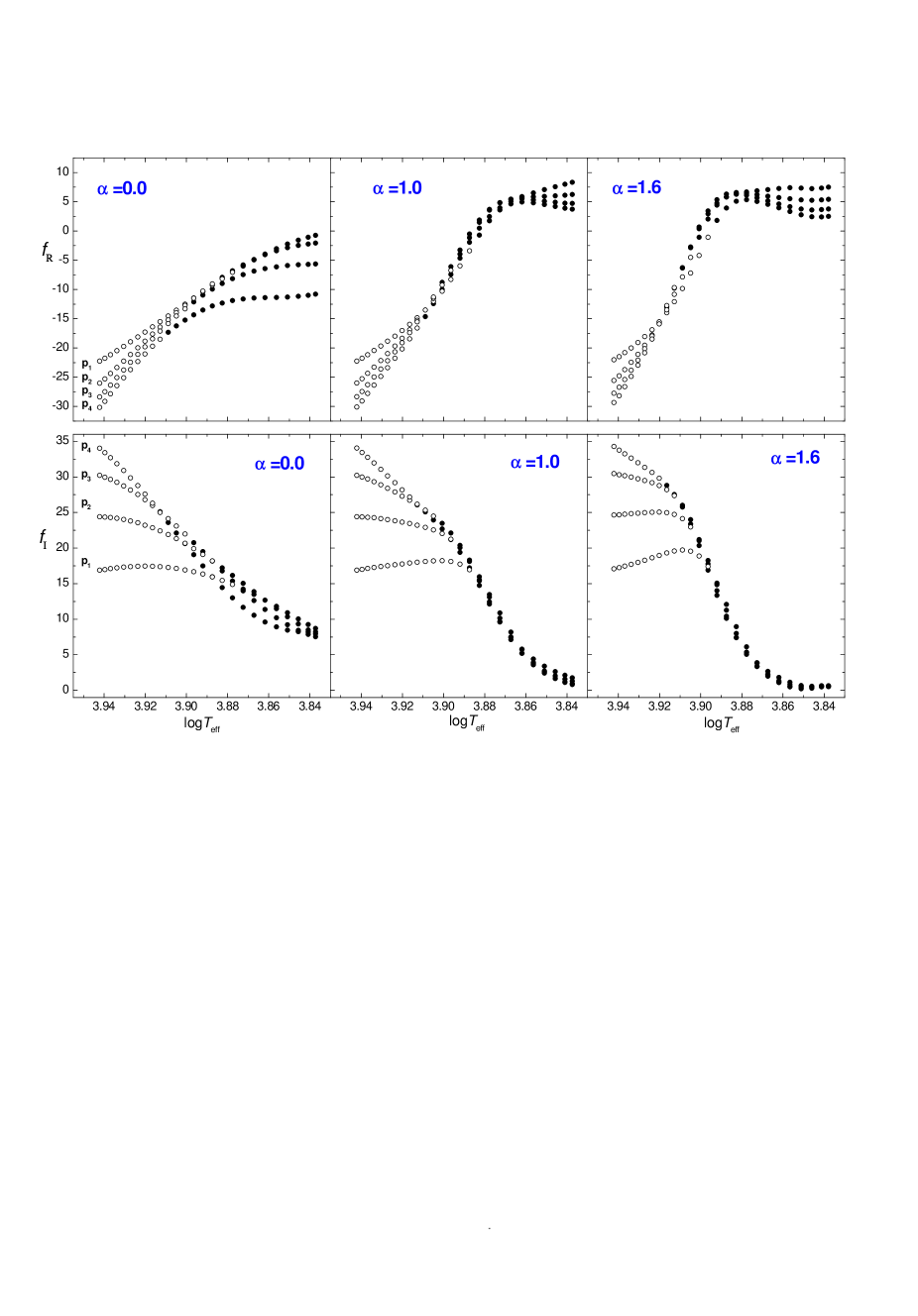
Figure 1: The real and imaginary part of the $f$-parameter for radial oscillation of a 1.9 $M_{\odot}$ star in the main-sequence phase. In the panels from left to right we show the $f$-parameter for three values of $\alpha$. Dots represent the unstable modes, whereas open circles the stable ones.

In the next section we demonstrate strong sensitivity of $f$ and, in a consequence, of mode position in the diagnostic diagrams, to the description of the convective flux. Our treatment of convection is very simplistic. We rely on the mixing-length theory and the convective flux freezing approximation. We study how calculated positions in the diagnostic diagrams vary with the changes of mixing-length parameter, $\alpha$.

Our method of inferring $f$ from the data is described in Sect. 3. The subsequent section presents application of the method to several $\delta$ Scuti stars. In the last section we summarize results of our analysis.

2 Calculated mode positions in the diagnostic diagrams

We use here the standard description of oscillating stellar photospheres (cf. Cugier et al. 1994). The local displacement is adopted in the form

$$\delta r(R,\theta,\varphi)=\varepsilon R{\rm Re}\{Y_{\ell}^{m}{\rm e}^{-{\rm i}\omega t}\},$$

where $\varepsilon$ is a small complex parameter fixing mode amplitude and phase. The associated perturbation of the bolometric flux, ${\cal F}_{\rm bol}$, and the local gravity, $g$, are then given by

$$\frac{\delta{\cal F}_{\rm bol}}{{\cal F}_{\rm bol}}=\varepsilon{\rm Re}\{fY_{\ell}^{m}{\rm e}^{-{\rm i}\omega t}\},$$

and

$$\frac{\delta g}{g}=-\left(2+\frac{\omega^{2}R^{3}}{GM}\right)\frac{\delta R}{R}.$$

With the static plane-parallel approximation for the atmosphere we can express the complex amplitude of the monochromatic flux variation as follows (see e.g. Daszyńska-Daszkiewicz et al. 2002)

$$A^{\lambda}(i)=\varepsilon Y_{\ell}^{m}(i,0)b_{\ell}^{\lambda}(D_{1,\ell}^{\lambda}+D_{2,\ell}+D_{3,\ell}^{\lambda}),$$

where $i$ is the inclination angle and $\lambda$ identifies the passband,

$$D_{1,\ell}^{\lambda}=\frac{1}{4}f\frac{\partial\log({\cal F}_{\lambda}|b_{\ell}^{\lambda}|)}{\partial\log T_{\rm{eff}}},$$

$$D_{2,\ell}=(2+\ell)(1-\ell),$$

$$D_{3,\ell}^{\lambda}=-\left(\frac{\omega^{2}R^{3}}{GM}+2\right)\frac{\partial\log({\cal F}_{\lambda}|b_{\ell}^{\lambda}|)}{\partial\log g}.$$

The disc averaging factor, $b_{\ell}$, is defined by the integral

$$b_{\ell}^{\lambda}=\int_{0}^{1}h_{\lambda}(\mu)\mu P_{\ell}(\mu)d\mu,$$

where the function $h_{\lambda}$ describes the limb darkening law and $P_{\ell}$ is the Legendre polynomial. The partial derivatives of ${\cal F}_{\lambda}|b_{\ell}^{\lambda}|$ may be calculated numerically from tabular data. Here we rely on Kurucz (1998) models and Claret (2000) computations of limb darkening coefficients. With Eq. 1 we can directly obtain the amplitude ratio and the phase difference for chosen pair of passbands, which are called nonadiabatic observables. Nonadiabaticity of oscillations enters through the complex parameter $f$, which is the central quantity of our paper.

In Fig. 1 we illustrate how the choice of the mixing-length parameter, $\alpha$, affects the value of $f$. We can see the large effect of the choice, particularly between $\alpha=0.0$ and $\alpha=1.0$ in the cooler part of the sequence where all modes are unstable. We have found that important is only the value of $\alpha$ in the H ionization zone. Models calculated with $\alpha$ fixed in this zone and varied in the HeII ionization zone yield very similar values of $f$.

In the next two figures we show how the differences in $\alpha$ are reflected in the $A_{b-y}/A_{y}\leavevmode\nobreak\ vs.\leavevmode\nobreak\ \varphi_{b-y}-\varphi_{y}$ diagram employing the Strömgren passbands . The effect of varying $\alpha$ is very large indeed. First, in Fig. 2 we show all the unstable modes in the frequency range covering $p_{1}$ to $p_{4}$ radial mode. The domains of different $\ell$’s partially overlap even at specified $\alpha$. The ambiguity is removed once model parameters are fixed, as seen in Fig. 3, but sensitivity to $\alpha$ is well visible. The sensitivity indicates that, if we are able to deduce values of $f$ from multi-color photometry, we will have at hand a valuable new constraints on stellar convection.

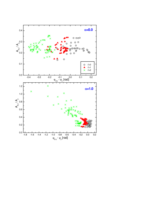
Figure 2: The effect of mixing-length parameter on the locations of modes with different $\ell$ degree. Here we show the positions of $\ell=0,1,2$ unstable modes in the diagnostic diagrams involving $b-y$ and $y$ Strömgren filters for $\delta$ Scuti models of $1.9M_{\odot}$. The frequency range covers $p_{1}$ to $p_{4}$ radial modes. The upper and lower panels are for $\alpha=0$ and $\alpha=1.0$, respectively.

The test should be applied to more realistic modeling of convection - pulsation interaction than used here. Our only aim here was to show sensitivity of the nonadiabatic observables to convection and we believe that our approximation is adequate for this aim. In section 4 we compare the calculated and measured $f$’s.

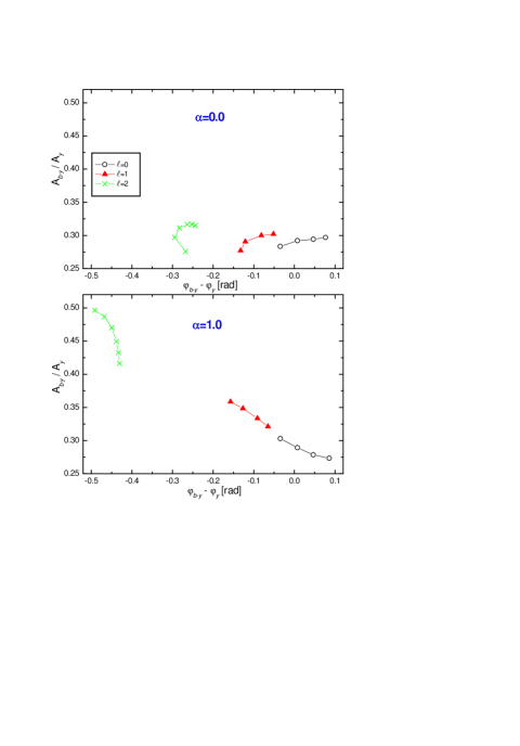
Figure 3: The same as in Fig. 2, but the one stellar model with $\log T_{\rm eff}=3.867$ is considered. The upper panel shows the photometric observables calculated at $\alpha=0.0$, and the lower one those at $\alpha=1.0$.

3 A method for inferring $f$ values from observations

We begin with rewriting Eq.1 in the form of the following linear equation.

$${\cal D}_{\ell}^{\lambda}({\tilde{\varepsilon}}f)+{\cal E}_{\ell}^{\lambda}{\tilde{\varepsilon}}=A^{\lambda}.$$

where

$${\tilde{\varepsilon}}\equiv\varepsilon Y^{m}_{\ell}(i,0),$$

$${\cal D}_{\ell}^{\lambda}f\equiv b_{\ell}^{\lambda}D_{1,\ell}^{\lambda},$$

$${\cal E}_{\ell}^{\lambda}\equiv b_{\ell}^{\lambda}(D_{2,\ell}+D_{3,\ell}^{\lambda}).$$

Here the $\lambda$ superscript identifies the passband. Eqs.(2) for a number of $\lambda$’s form a set of observational equations. In the right-hand side we have measured amplitudes, $A^{\lambda}$, expressed in the complex form. The quantities to be determined are $({\tilde{\varepsilon}}f)$ and ${\tilde{\varepsilon}}$. Both must be regarded complex. Of course we are primarily interested in the value of $f$. However, inferred value of $\tilde{\varepsilon}$ may also be useful as a constraint on mode identification if it is found unacceptably large.

Table 1: Stellar parameters for three $\delta$ Sct stars: $\beta$ Cas, 20 CVn and AB Cas.

Object	Sp	Period [d]	$\pi$ [mas]	$\log T_{\rm eff}$	$\log L$	$\log g*$	$\log g**$	[m/H]	$v_{e}\sin i$
$\beta$ Cas	F2III-IV	0.1009	$59.89\pm 0.56$	$3.856\pm 0.01$	$1.426\pm 0.008$	$3.60\pm 0.01$	3.66	0.0	69
20 CVn	F3III	0.1217	$11.39\pm 0.69$	$3.874\pm 0.01$	$1.881\pm 0.053$	$3.62\pm 0.01$	3.49	0.5	15
AB Cas	A3V+KV	0.0583	$3.33\pm 1.30$	$3.908\pm 0.01$	$0.998\pm 0.430$	$4.55\pm 0.01$	4.26	0.0	55

$*$ from photometry        $**$ from evolutionary tracks

Having data only for two passbands we can infer $f$ in a unique way once we know $\ell$. However, we usually do not and therefore we need at least three passband data. The procedure is to determine $f$ by means of $\chi^{2}$ minimization, assuming trial values of $\ell$. We will regard the $\ell$ and the associated complex $f$ value as the solution if it corresponds to $\chi^{2}$ minimum which is significantly deeper than at other $\ell$’s. We will consider the $\ell$ values up to six.

If we have data on spectral line variations, the set of equations (2) may be supplemented with an expression relating $\tilde{\varepsilon}$ to complex amplitudes of the first moments, ${\cal M}_{1}^{\lambda}$,

$$-{\rm i}\omega R\left(u_{\ell}^{\lambda}+\frac{GMv_{\ell}^{\lambda}}{R^{3}\omega^{2}}\right)\tilde{\varepsilon}={\cal M}_{1}^{\lambda}.$$

where

$$u_{\ell}^{\lambda}=\int_{0}^{1}h_{\lambda}(\mu)\mu^{2}P_{\ell}(\mu)d\mu.$$

$$v_{\ell}^{\lambda}=\ell\int_{0}^{1}h_{\lambda}(\mu)\mu\left(P_{\ell-1}(\mu)-\mu P_{\ell}(\mu)\right)d\mu.$$

are coefficients representing a straightforward generalization of the coefficients $u_{\ell}$ and $v_{\ell}$ introduced by Dziembowski (1977) for gray atmospheres. We stress that the first moment is the only measure of the radial velocity amplitude, which does not depend on the aspect and the azimuthal number, $m$, just like the light amplitude.

There are uncertainties in model parameters, which enter the expressions for $D_{1}^{\lambda}$ and $D_{3}^{\lambda}$. The partial derivatives of ${\cal F}_{\lambda}|b_{\ell}^{\lambda}|$, which appear there depend on $T_{\rm eff}$, $\log g$ and the metallicity parameter $[m/H]$. We will not consider here the stars with chemical peculiarities, thus we are adopting the solar mixtures of heavy elements. We repeat our minimization for the ranges of these three parameters consistent with observational errors as well as with our evolutionary tracks.

If the best fit is for $\ell=0$, an additional constraint on models follows from mode frequency, because the $\ell=0$ frequency spectrum is sparse and the radial order of the mode may be easily identified. In this case we can tune a star in the exact values of the observed frequency. Stellar parameters have significant effect on $\chi^{2}$. We will see that based on $\chi^{2}$ we can obtain more stringent constrains on these parameters.

Generalization of the method to the case of modes coupled by rotation is straightforward. Such modes are represented in terms of a superposition of spherical harmonics with $\ell$’s differing by 2 and the same $m$’s. The monochromatic amplitude of a coupled mode is given by

$${\mathcal{A}}^{\lambda}(i)=\sum_{k}a_{k}A_{k}^{\lambda}(i)$$

where $a_{k}$ coefficients are solutions of the degenerate perturbation theory for slowly rotating stars (see Daszyńska-Daszkiewicz et al. 2002). The values of $a_{k}$ coefficients depend on the rotation rate and the frequency distance between modes.

The counterpart of Eq.(2) is

$$\sum_{k}w_{k}^{\lambda}[{\cal D}_{\ell_{k}}^{\lambda}(\varepsilon f)+{\cal E}_{\ell_{k}}^{\lambda}\varepsilon]=A^{\lambda},$$

where

$$w_{k}^{\lambda}=Y^{m}_{\ell_{k}}(i,0)b_{\ell_{k}}^{\lambda}a_{k}.$$

The main difference relative to the single $\ell$ case is that now the result depends on the aspect. Further, we expect a strong dependence of calculated amplitude on model parameters because the values of $a_{k}$ are very sensitive to small frequency distances between coupled modes.

4 Applications

We applied the method described above to data on three $\delta$ Sct variables: $\beta$ Cas, 20 CVn and AB Cas. In Table 1 we give parameters for these stars. In this table we rely mostly on the catalogue of Rodriguez et al. (2000).

The photometric data were dereddened according to Crawford (1979) and Crawford & Mandwewala (1976), and then the effective temperatures, gravities and bolometric corrections were obtained from Kurucz’s (1998) tabular data. In Table 1 we give two values of $\log g$, from Kurucz data and from evolutionary tracks. To calculate the $D_{1}^{\lambda}$ and $D_{3}^{\lambda}$ coefficients we took the second one, which we regard more reliable. Errors in $\log T_{\rm eff}$ and $\log g$ correspond to typical errors from the photometric calibration procedure.

For $\beta$ Cas and AB Cas we adopted solar metal abundance, whereas for 20 CVn we used $[m/H]=0.5\leavevmode\nobreak\ (Z\approx 0.06)$ due to Hauck et al.(1985) and Rodriguez et al.(1998) and checked also the other one, $[m/H]=0.3\leavevmode\nobreak\ (Z\approx 0.04)$. The values of $\log L$ for $\beta$ Cas and 20 CVn are derived from the Hipparcos parallaxes. The parallax for AB Cas is very inaccurate. The central value locates this object close to the ZAMS. Though the star is a component of an Algol-type binary system, it is reasonable to assume that it is described by ordinary mass-conserving models because it was originally less massive and the episode of the rapid mass accretion is most likely forgotten. This is what we assume in this paper. Therefore, we adopted as the minimum luminosity the value at ZAMS, and the maximum luminosity as the highest values allowed by the Hipparcos parallax.

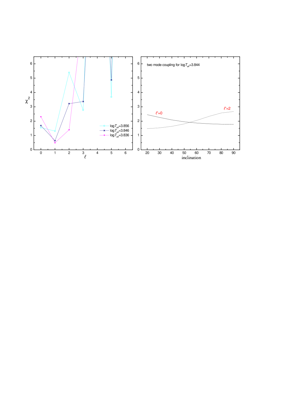
Figure 4: In the left panel we show the $\chi^{2}$ as a function of $\ell$ obtained for three models of $\beta$ Cas star. In the right panel we plot the $\chi^{2}$ as a function of inclination considering the mode coupling between $\ell=0$ and $\ell=2$ at $v_{\rm rot}=$70 km/s.

4.1 $\beta$ Cas

$\beta$ Cas is a $\delta$ Sct star with radial velocity variations of 2 km/s (Mellor 1917). Mills (1966) classified it as $\delta$ Sct variable on the basis of photometric observations.

$\beta$ Cas is one of a few $\delta$ Sct stars in which only one mode has been detected so far. Rodriguez et al. (1992) identified this mode as $p_{2}$ or $p_{3}$ of $\ell=1$, on the basis of photometric diagrams in Strömgren filters. Balona & Evers (1999), using the same photometric data, did not get an unambiguous identification.

We have rather precise parameters for this, the brightest and the nearest $\delta$ Scuti variable. Note, in particular, small luminosity errors in Tab. 1. The adopted metal abundance, $Z=0.02$, is based on the $[m/H]$ value obtained from IUE spectra by Daszyńska & Cugier (2002). The photometric amplitudes and phases are from Rodriguez et al. (1992).

The frequency value combined with mean density implies that if the mode were radial, it could be only $p_{3}$. We first assume that the mode is adequately described in terms of single spherical harmonic and consider $\ell$-values from 0 to 6. The uncertainties in the values of $M$ and $R$ are inconsequential and we consider only uncertainty in $T_{\rm eff}$. The estimated value of the mass is $1.95M_{\odot}$. In the left panel of Fig. 4 we see that the uncertainty on the effective temperature does not impair identification of the $\ell$ value. The $\chi^{2}$ minimum at $\ell=1$ is the deepest one, particularly at the two lower effective temperatures.

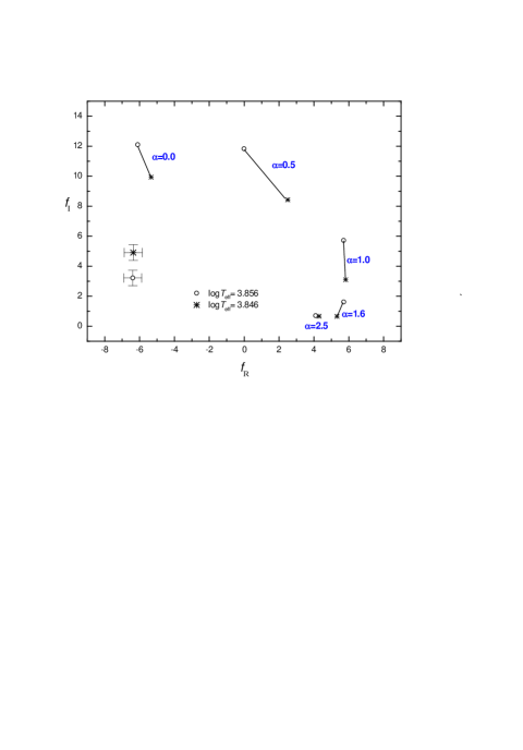
Figure 5: Comparison of the $f$ values inferred from Strömgren photometry for $\beta$ Cas with the values from the models calculated with various values of the MLT parameter $\alpha$ and the mass of $1.95M_{\odot}$. Points with the error bars represent inferred values assuming two indicated effective temperatures.

The star is a relatively rapid rotator, $v_{\rm rot}$ is at least 70 km/s, therefore we have to consider the possibility that the mode is a coupled one, most likely an $\ell=0$ and $\ell=2$ superposition (see Daszyńska-Daszkiewicz at al. 2002). Relying on the formalism described at the end of Section 3, we evaluated the best $f$-values and assiociated $\chi^{2}$ as a function of the aspect. In the right panel we show $\chi^{2}$ variation with the inclination. We can see that at no value of the inclination the $\chi^{2}$ is nearly as low as at $\ell=1$. Thus we conclude that the mode excited in $\beta$ Cas is most likely a single $\ell=1$ mode.

Values of $f$ corresponding to this identification are shown in Fig. 5 together with the error bars, which are the errors from the least-square method. The uncertainty in temperature is more significant than the errors of $f$ determination. The theoretical $f$ values were calculated for $M=1.95M_{\odot}$ assuming five values of the mixing-length parameter $\alpha$: 0.0, 0.5, 1.0, 1.6 and 2.5. Still the constraint on convection is interesting because the range of the acceptable values of $f$ is narrower than the range of the calculated values with different $\alpha$’s.

The observed values of $f_{R}$ are closer to those calculated with $\alpha=0$, which may be taken as an evidence that convection in the H ionization zone is relatively inefficient. However, values of $f_{I}$ require rather higher $\alpha$’s (about 1) instead. In view of our crude treatment of convection–pulsation interaction we have to take these indications with a great caution.

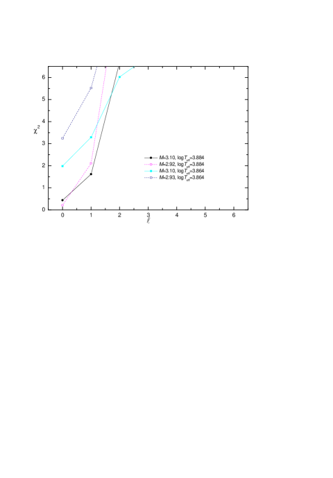
Figure 6: Dependence of $\chi^{2}$ on $\ell$ for four models of 20 CVn on the edges of the error box obtained for $Z=0.06$.

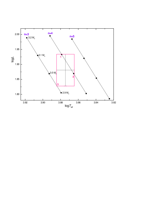
Figure 7: The observational error box for 20 CVn on HR diagram. The lines of constant radial order, $n=3,4,5$, are also drawn.

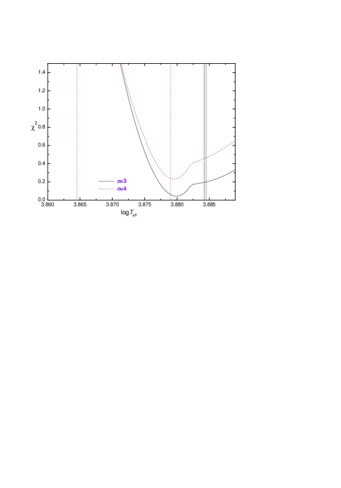
Figure 8: The variation of $\chi^{2}$ with effective temperature for the models along the lines $n=3$ and $n=4$.

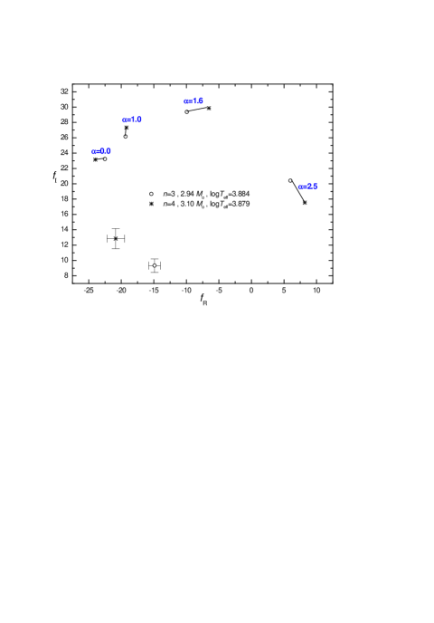
Figure 9: The same as in Fig. 5, but with empirical values of $f$ for the models with min$\chi^{2}$ for $n=3$ and $n=4$ of 20 CVn.

4.2 20 CVn

This $\delta$ Scuti variable is also regarded to be monoperiodic (e.g. Shaw 1976, Peña & Gonzalez-Bedolla 1981). The mode was identifited as $\ell=0$ by means of photometry (Rodriguez et al. 1998) as well as spectroscopy (Chadid et al. 2001). Our result shown in Fig. 6 for $Z=0.06$ clearly confirms the previous identification. For models on the edges of the error box the minimum of $\chi^{2}$ is at $\ell=0$. The same is true for $Z=0.04$, but the values of the $\chi^{2}$ are higher.

As we mentioned in Sect. 2, having such identification of pulsating mode we can refine stellar parameters by fitting the observed period. Still, we have to consider various radial orders, $n$. In Fig. 7 we show the HR diagram with the error box representing uncertainty of stellar parameters and the lines of the constant period ($P$ = 0.1217 d) for $n=3,4,5$, obtained with evolutionary models calculated for $Z=0.06$ and indicated masses. Only models along these lines are allowed. We can see that as for the radial order we have only two possibilities, $n=3$ or $n=4$. In the case of $Z=0.04$ only $n=4$ is allowed but the $\chi^{2}$ is significantly larger. We thus see that our method allows to constrain the $Z$ value.

In Fig.8 we show the variations of the $\chi^{2}$ with $\log T_{\rm eff}$ for the tuned models with $n=3$ and $n=4$. The vertical lines correspond to the intersections of the constant period lines with the error box, so that only the values of $\log T_{\rm eff}$ between these lines for a given $n$ are allowed. The models yielding the lowest $\chi^{2}$ are just models 1 and 3 in Fig.7 for $n=4$ and $n=3$, respectively. The values of $\chi^{2}$ are 0.19 for $n=3$ and 0.24 for $n=4$, what indicates that both are possible as identifications of the radial order in this star.

Fig. 9 shows the empirical values of the nonadiabatic $f$-parameter for models corresponding to the deepest $\chi^{2}$ minima for four values of $\alpha$: 0.0, 1.0, 1.6 and 2.5. Relative positions of empirical and theoretical $f$ values in 20 CVn are qualitatively similar to those in $\beta$ Cas (cf. Fig. 5). However, these values, both calculated and inferred, are considerably higher than in the case of $\beta$ Cas, which is a consequence of higher radial order. The $\ell=1$ mode identified in $\beta$ Cas has frequency between the $n=2$ and $n=3$ radial modes.

4.3 AB Cas

The next example is the primary component of an Algol-type system. As we have already pointed out, luminosity of this star is very uncertain due to the large error in the parallax. We will see that with our method we can significantly improve the accuracy of the stellar parameters as provided that the identified mode is radial.

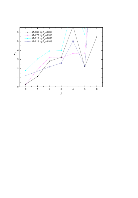
Figure 10: Dependence of $\chi^{2}$ on $\ell$ for four models on the edges of the error box of AB Cas.

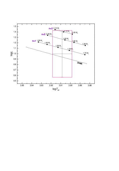
Figure 11: The observational error box for AB Cas on HR diagram. The lines of constant radial order with $n=1,2,3$ are also shown.

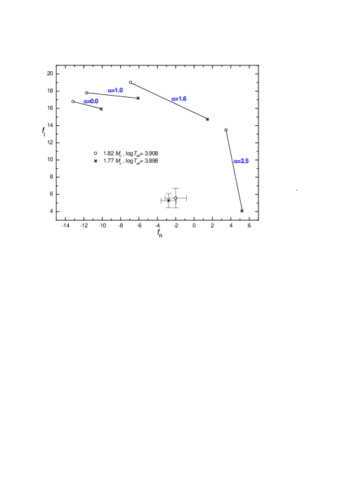
Figure 12: The same as in Fig. 5, but with empirical values of $f$ for two tuned models of AB Cas with $n=1$ and $\log T_{\rm eff}=3.908$ and 3.898.

In the whole range of allowed parameters $\chi^{2}$ has by far the deepest minimum at $\ell=0$, as we can see in Fig. 10. This identification is in agreement with that of Rodriguez et al. (1998). In Fig. 11 we show the HR diagram with the error box representing uncertainty of stellar parameters and the lines of the constant period ($P$ = 0.0583 d) for $n=1,2,3$, obtained with evolutionary models calculated for $Z=0.02$ and indicated masses. The deepest minimum of $\chi^{2}$ (0.25) along the $n=1$ line occurs at $M=1.77,\log T_{\rm eff}=3.8985,\log L=1.047$. The lowest value of $\chi^{2}$ for $n=2$ (0.62) is at $M=1.91,\log T_{\rm eff}=3.8985,\log L=1.217$, and for $n=3$ we got $\chi^{2}=1.02$, $T_{\rm eff}=3.8985,\log L=1.361$. We can see that $n=1$ identification is strongly favored. For such mode identification the value of $\log L$ is between 1.047 and 1.144 leading to $\chi^{2}=0.25$ and 0.56, respectively.

In Fig. 12 we compare empirical values of $f$ with ones calculated for various mixing-length parameter, $\alpha$. The star is the hottest of the three objects. Still, calculated values are strongly affected by the choice of $\alpha$. Just like the previous, regardless the value of $\alpha$, the empirical values of the real and imaginary parts of $f$, could not be simultaneously reproduced with our model calculations.

5 Conclusions and discussion

We believe that the three examples of $\delta$ Scuti stars considered in the previous section, clearly show that there is a wider application of multicolor data on excited mode than explored so far. In addition to the spherical harmonic degree, $\ell$, we were able with our $\chi^{2}$ minimization method to infer the value of the complex parameter $f$ which describes the bolometric flux perturbation and yields a strong constraint on models of stellar convection. In the two cases when determined value of $\ell$ was zero, we were able to determine the radial order of the mode and significantly limit the uncertainty of the stellar parameters.

The values of $f$ we found could not be reproduced with model calculations made with the convective-flux-freezing approximation for any value of the MLT parameter $\alpha$. We should not be surprised. After all, the approximation adopted is grossly inadequate. Though there are certain common features in the relative positions of the deduced and calculated $f$’s in the three cases considered, it is premature to draw any conclusions about properties of stellar convection from this fact.

Inadequacy in our treatment of convection is not the only possible cause of the large discrepancy between the calculated and empirical $f$’s. Our use of the Eddington approximation in calculation of the nonadiabatic oscillations may be an oversimplification. We believe it is of secondary importance as the value of $f$ is determined at the optical depth $\tau\gg 1$. Our use of static atmospheric models with the depth-independent $g$ seems also a good approximation. Still, it should be kept that these two approximation should be at some point verified. The accuracy of the atmospheric models is of a greater concern, which was discussed recently by Heiter et al.(2002), where sensitivity of the atmospheric structure and observable quantities to the convection treatment was demonstrated (see also Smalley & Kupka 1997). Whatever is the cause of discrepancy, the goal in model calculations should be to achieve consistent $f$’s.

Determination of $\ell$ is an independent goal. It is important that it could be done without an a priori knowledge of $f$. This is not a new finding. This has been done earlier for both $\delta$ Scuti and $\beta$ Cephei variables. In particular, in the latter case, when $f$ may be approximately treated as real, the three color data often allow for an unambiguous $\ell$ determination (e.g. Heynderickx et al. 1994, Balona& Evers 1999 ). For $\delta$ Scuti stars the situation is more complicated. Although, we believe, our method represents an improvement, it still does not always work . We may believe in the inferred values of both $f$ and $\ell$ only if the minima of $\chi^{2}$ are strongly $\ell$ dependent. This was the true in all the three cases considered in the previous section. It is not always so. For the $\delta$ Scuti star 1 Mon, for instance, we found $\chi^{2}$ quite flat between $\ell=0$ and 2. For this star we also made an unsuccessful attempt to use the data of the radial velocity as provided by Balona et al.(2001), but even including this quantity did not change the result. This failure should not discourage future efforts to combine spectroscopic data.

The main message of our work is that applications of multi-color photometry data of $\delta$ Scuti stars go beyond identification of the $\ell$ values of the excited mode. We showed that such data allow to refine parameters of the stars and, what we regard most important, yield strong constraints on models of stellar convection.

- (1) Balona L. A., Evers E. A., 1999, MNRAS 302, 349
- (2) Balona L. A., Bartlett B., Caldwell J. A. R. et al., 2001, MNRAS 321, 239
- (3) Breger M., Pamyatnykh A. A., Pikall H., Garrido R., 1999, A&A 341, 151
- (4) Chadid M., De Ridder J., Aerts C., Mathias P., 2001, A&A 375, 113
- (5) Crawford D.L., 1979, AJ 84, 1858.
- (6) Crawford D.L., Mandwewala N., 1976, PASP 88, 917.
- (7) Cugier H., Dziembowski W. A., Pamyatnykh A. A., 1994, A&A 291, 143
- (8) Claret A., 2000, A&A 363,1081
- (9) Daszyńska J., Cugier H., 2002, COSPAR 2000, Adv. Space Res. 31, 381
- (10) Daszyńska-Daszkiewicz J., Dziembowski W. A., Pamyatnykh A. A., Goupil M-J. 2002, A&A 392, 151
- (11) Dziembowski W. A.,1977, Acta Astron. 27, 203
- (12) Garrido R., 2000, in Breger M., Montgomery M. H., eds, Delta Scuti and Related Stars, ASP Conf. Ser. 210, 67
- (13) Hauck B., Foy R., Proust D., 1985, A&A 149,167
- (14) Heiter U., Kupka F., van’t Veer-Menneret C. et al., 2002, A&A 392, 619
- (15) Heynderickx D., Waelkens C., Smeyers P., 1994, A&AS 105, 447
- (16) Koen C., Balona L., van Wyk F., Marang F., Paunzen E., 2002, MNRAS 330, 567
- (17) Kurucz, R. L., 1998, http://cfaku5.harvard.edu
- (18) Mellor L.L., 1917, Publ. Obs. Univ. Mich. 3, 16
- (19) Millis R.L., 1966, PASP 78, 340
- (20) Peña J.H., Gonzalez-Bedolla S.F., 1981, AJ 86, 1679
- (21) Rodriguez E., Rolland A., López de Coca P., Garrido R., González-Bedolla S. F., 1992, A&AS 96, 429
- (22) Rodriguez E., Claret A., Sedano J.L. et al., 1998, A&A 340, 196
- (23) Rodriguez E., López-González, M. J., López de Coca P., 2000, in Breger M., Montgomery M. H., eds, Delta Scuti and Related Stars, ASP Conf. Ser. 210, 499
- (24) Rodriguez E., Rolland A., Garrido R. et al. 1998, A&A 331, 171
- (25) Rodriguez E., Rolland A., López-González M. J., López de Coca P., 2000, A&AS 144, 469
- (26) Shaw J.S., 1976, AJ 81, 661
- (27) Smalley B., Kupka F., 1997, A&A 328, 349