The Angular Power Spectrum of EDSGC Galaxies

Abstract

We determine the angular power spectrum $C_{l}$ of the Edinburgh/Durham Southern Galaxy Catalog (EDSGC) and use this statistic to constrain cosmological parameters. Our methods for determining $C_{l}$ and the parameters that affect it are based on those developed for the analysis of cosmic microwave background maps. We expect them to be useful for future surveys. Assuming flat cold dark matter models with a cosmological constant (constrained by COBE/DMR and local cluster abundances) and a scale–independent bias $b$, we find acceptable fits to the EDSGC angular power spectrum with $1.11<b<2.35$ and $0.2<\Omega_{m}<0.55$ at 95% confidence. These results are not significantly affected by the “integral constraint” or extinction by interstellar dust, but may be by our assumption of Gaussianity.

Submitted to ApJ

1 Introduction

Over the next decade, the quantity and quality of galaxy survey data will improve greatly because of a variety of new survey projects underway including the Sloan Digital Sky Survey (SDSS; see York et al. 2000). However, most of the galaxies in such surveys will not have spectroscopically–determined redshifts; therefore, the study of their angular correlations will be highly profitable for our understanding of the large–scale structure of the Universe.

The primary purpose of this paper is to consider an analysis approach which is likely to be useful for deriving cosmological constraints from these larger surveys. In particular, we use methods that have become standard in the analysis of cosmic microwave background (CMB) anisotropy maps, such as those from Boomerang (de Bernardis et al. 2000; Lange et al. 2000) and Maxima-I (Hanany et al. 2000, Balbi et al. 2000).

Estimation of the two–point angular correlation function $w(\theta)$ from galaxy surveys without redshfit information has a long history. Early work (Peebles & Hauser 1974; Groth & Peebles 1977) found the angular correlation function to vary as $w(\theta)=\theta^{1-\gamma}$ with $\gamma=1.77$ and a break at scales larger than $\sim 9{\,{\rm h}^{-1}~{}\rm Mpc}$. The advent of automated surveys, such as the APM galaxy survey (Maddox et. al. 1990) and Edinburgh/Durham Southern Galaxy Catalogue (EDSGC; Collins, Nichol & Lumsden 1992) enabled a much more accurate determination of $w(\theta)$, as each survey contained angular positions for over a million galaxies.

One way to compare the measured angular correlation function with theoretical predictions is to invert $w(\theta)$ to obtain the three–dimensional power spectrum $P(k)$. This requires inverting Limber’s equation (Limber 1953). Baugh & Efstathiou (1993, 1994) and Gaztañaga & Baugh (1998) used Lucy’s algorithm (Lucy 1974) to do the inversion, while Dodelson & Gaztañaga (2000) used a Bayesian prior constraining the smoothness of the power spectrum. Eisenstein & Zaldarriaga (2000) used a technique based on singular-value decomposition to get $P(k)$ from $w(\theta)$. They point out that, once the correlations in the inverted power spectra are included, the uncertainties on cosmological parameters from the APM are significantly weakened.

Our analysis is a three-step process, similar to what is done with CMB data sets (Tegmark 1997; Bond, Jaffe & Knox 1998; Bond, Jaffe & Knox 2000). The first step is the construction of a pixelized map of galaxy counts, together with its noise properties. The second step is the determination of the angular power spectrum $C_{l}$ of the map using likelihood analysis, together with window functions and a covariance matrix. In the final step, we compare our observationally–determined $C_{l}$ to the $C_{l}$ predicted for a given set of parameters in order to get constraints on those parameters. We assume that the errors in $C_{l}$ are log–normally distributed.

The angular power spectrum $C_{l}$ is a useful intermediate step on this road from galaxy catalog to parameter constraints. Estimates of the angular power spectrum, together with a description of the uncertainties, can be viewed as a form of data compression. One has converted the $\sim\!1$ million EDSGC galaxies (for example) into a handful of power spectrum constraints, together with window functions and covariance matrices. Thus if one wishes to make other assumptions about bias and cosmological parameters than we have done here and determine the resulting constraints, one can do so without having to return to the cumbersome galaxy catalog.

We use $C_{l}$ instead of its historically–preferred Legendre transform $w(\theta)$ for several reasons. First, the error matrix structure is much simpler: $\langle\delta C_{l}\delta C_{l^{\prime}}\rangle$ is band-diagonal and becomes diagonal in the limit of full–sky coverage, whereas $\langle\delta w(\theta)\delta w(\theta^{\prime})\rangle$ is much more complicated and does not become diagonal even in the full–sky limit. Second, the relation between $C_{l}$ and the corresponding three–dimensional statistic $P(k)$ is simpler than that between $w(\theta)$ and $P(k)$ (or its Fourier transform $\xi(r)$ (Baugh & Efstathiou 1994)).

We use likelihood analysis to determine $C_{l}$ because the likelihood is a fundamental statistical quantity. The likelihood is the probability of the data given $C_{l}$, which by Bayes’ theorem is proportional to the probability of $C_{l}$ given the data. Another advantage of likelihood analysis is that, as explained below, it allows for straightforward control of systematic errors (due to, e.g., masking) via modifications of the noise matrix.

Only on sufficiently large scales do we expect the likelihood function to be a Gaussian that depends only on $C_{l}$ and not any higher-order correlations. We therefore restrict our analysis to $l$ values less than some critical value. On small scales the likelihood function becomes much more complicated and its form harder to predict a priori. Mode-mode coupling due to nonlinear evolution leads to departures of the $C_{l}$ covariance matrix from band-diagonal. Therefore some of the advantages of likelihood analysis and the angular power spectrum are lost on smaller scales where other techniques may be superior. The Gaussianity assumption is perhaps the weakest point of the approach outlined here. Below, we briefly discuss how the analysis can be improved in this regard with future data sets.

The EDSGC, with over a million galaxies and covering over 1000 sq. degrees, offers us an excellent test bed for applying our algorithms (Nichol, Collins & Lumsden 2000). We convert this catalog into a pixelized map and determine its angular power spectrum together with window functions and covariance matrix. As an illustrative application of the angular power spectrum, we constrain a scale–independent bias parameter $b$ and the cosmological constant density parameter $\Omega_{\Lambda}$ in a COBE–normalized $\Lambda$CDM model with zero mean spatial curvature. Our constraints on the bias are improved by including constraints on the amplitude of the power spectrum derived from number densities of low–redshift massive clusters of galaxies (Viana & Liddle 1999, hereafter VL99; also see Pierpaoli, Scott & White 2000). These number densities are sensitive to the amplitude of the matter power spectrum calculated in linear perturbation theory, near the range of length scales probed by the EDSGC.

The angular power spectrum of the APM catalog was previously estimated by Baugh & Efstathiou (1994) though not via likelihood analysis. Very recently, Efstathiou & Moody (2000) have applied the same techniques we do here to estimating $C_{l}$ for the APM survey. Their approach differs from ours in how they constrain cosmological parameters. Instead of projecting the theoretical three–dimensional power spectra $P(k)$ into angular power spectra, they transform their $C_{l}$ constraints into (highly correlated) constraints on $P(k)$ and then compare to theoretical $P(k)$.

We expect the analysis methods presented here to be useful for other current and future data sets—even those with large numbers of measured redshifts. For example, the Sloan Digital Sky Survey (SDSS) will spectroscopically determine the redshifts of a million galaxies, but there will be about one hundred times as many galaxies in the photometric data, without spectroscopic redshifts. One can generalize the methods presented here to analyze sets of maps produced from galaxies in different photometric redshift slices.

In §2, we review likelihood analysis and the use of the quadratic estimator to iteratively find the maximum of the likelihood function. In §3 we describe our calculation of $P(k)$ and its projection to $C_{l}$. In §4 we show how to compare the calculated $C_{l}$ to the measured $C_{l}$ in order to determine parameters. In §5 we apply our methods to the EDSGC, and discuss some possible sources of systematic error in §6. This is followed by a discussion of our results in §7 and a brief conclusion in §8. An appendix outlines the derivation of the projection of $P(k)$ to $C_{l}$.

2 The likelihood function and quadratic estimation

The likelihood is a fundamental statistical quantity: the probability of the data given some theory. According to Bayes’ theorem, the probability of the parameters of the assumed theory is proportional to the likelihood times any prior probability distribution we care to give the parameters. Thus, determining the location of the likelihood maximum and understanding the behavior of the likelihood function in that neighborhood (i.e., understanding the uncertainties) is of great interest.

Despite its fundamental importance, an exact likelihood analysis is not always possible. Two things can stand in our way: insufficient computer resources for evaluation of the likelihood function (operation count scales as $N_{\rm pix}^{3}$ and memory use scales as $N_{\rm pix}^{2}$), and, even worse, the absence of an analytic expression for the likelihood function.

In this paper we assume that the pixelized map of galaxy counts is a Gaussian random field—an assumption which provides us with the analytic expression for the likelihood function. For models with Gaussian initial conditions (which are the only models we consider here), we expect this to be a good approximation on sufficiently large scales. Since we restrict ourselves to studying large-scale fluctuations, we can use large pixels, thereby reducing $N_{\rm pix}$ and ensuring that the likelihood analysis is tractable. We also check the Gaussianity assumption with histograms of the pixel distribution. On the large scales of interest here and for a given three-dimensional length scale, Gaussianity is a better approximation for a galaxy count survey than for a redshift survey, due in part to the redshift-space distortions which affect the latter (Hivon et al. 1995). The projection from 3 dimensions to 2 dimensions also tends to decrease non-Gaussianity.

Where likelihood analysis is possible, it naturally handles the problems of other estimators (such as edge effects). Likelihood analysis also provides a convenient framework for taking into account various sources of systematic error, such as spatially varying reddening and the “integral constraint” discussed in §6.

To begin our likelihood analysis, we assume that the data are simply the angular position of each galaxy observed—though it is possible to generalize the following analysis and use either magnitude information or color redshifts. We pixelize the sky and count the number of galaxies in each pixel $G_{i}$. Then we calculate the fractional deviation of that number from the ensemble average:

$$\Delta_{i}\equiv{G_{i}-\bar{G}\Omega_{i}\over\bar{G}\Omega_{i}}$$ (1)

where $\bar{G}$ is the ensemble average number of galaxies per unit solid angle and $\Omega_{i}$ is the pixel solid angle. We do not actually know the ensemble mean. In practice, we approximate it with the survey average $\tilde{G}$. We discuss this approximation in §6 and demonstrate that it has negligible impact on our results.

We model the fractional deviation in each pixel from the mean as having a contribution from “signal” and from “noise”, so that

$$\Delta_{i}=s_{i}+n_{i}.$$ (2)

The covariance matrix, $C_{ij}$, for the fractional deviation in each pixel from the mean is given by:

$$C_{ij}\equiv\langle\Delta_{i}\Delta_{j}\rangle=S_{ij}+N_{ij}$$ (3)

where $S_{ij}\equiv\langle s_{i}s_{j}\rangle$ and $N_{ij}\equiv\langle n_{i}n_{j}\rangle$ are the signal and noise covariance matrices. Roughly speaking, signal is part of the data that is due to mass fluctuations along the line-of-sight (see the appendix), and noise are those fluctuations due to anything else.

The signal covariance matrix $S_{ij}$ depends on the parameters of interest (the angular power spectrum $C_{l}$) via:

$$S_{ij}=w(\theta_{ij})=\sum_{l}{2l+1\over 4\pi}C_{l}P_{l}\left(\cos\theta_{ij}\right)e^{-l^{2}\sigma_{b}^{2}}$$ (4)

where $\theta_{ij}$ is the angular distance between pixels $i$ and $j$ and we have assumed a Gaussian smoothing of the pixelized galaxy map with fwhm $=\sqrt{8ln2}\sigma_{b}$. In practice, we do not estimate each $C_{l}$ individually but binned $C_{l}$s with bin widths greater than $\sim\pi/\theta$ where $\theta$ is a typical angular dimension for the survey.

The noise contribution to the fluctuations $n$ is due to the fact that two regions of space with the same mass density can have different number of galaxies. We model this additional source of fluctuations as a Gaussian random process with variance equal to $1/\bar{G}$, so that

$$N_{ij}\equiv\langle n_{i}n_{j}\rangle=1/\bar{G}\,\delta_{ij}.$$ (5)

More sophisticated modeling of the noise is not necessary because at all $l$ values of interest, the variance in $C_{l}$ due to the noise is much smaller than the sample variance.

To find the maximum of the likelihood function, we iteratively apply the following equation:

$$\delta{\cal C}_{l}={1\over 2}F^{-1}_{ll^{\prime}}{\rm Tr}\left[(\Delta\Delta^{T}-C)(C^{-1}\partial C/\partial{\cal C}_{l^{\prime}}C^{-1})\right],$$ (6)

where $F$ is the Fisher matrix given by

$$F_{ll^{\prime}}={1\over 2}{\rm Tr}\left(C^{-1}{\partial C\over\partial{\cal C}_{l}}C^{-1}{\partial C\over\partial{\cal C}_{l^{\prime}}}\right),$$ (7)

and for later convenience we are using ${\cal C}_{l}\equiv l(l+1)C_{l}/(2\pi)$ instead of $C_{l}$. That is, start with an initial guess of ${\cal C}_{l}$, update this to ${\cal C}_{l}+\delta{\cal C}_{l}$, and repeat. We have found that this iterative procedure converges to well within the size of the error bars quite rapidly.

The small sky coverage prevents us from determining each multipole moment individually; thus we determine the power spectrum in bands of $l$ instead, call them “band powers”, and denote them by ${\cal C}_{B}$ where

$${\cal C}_{l}\equiv{l(l+1)C_{l}\over 2\pi}=\sum_{B}\chi_{B(l)}{\cal C}_{B}$$ (8)

and $\chi_{B(l)}$ is unity for $l_{<}(B)<l<l_{>}(B)$ where $l_{<}(B)$ and $l_{>}(B)$ delimit band $B$.

Although we view equation (6) as a means of finding the maximum of the likelihood function, one can also treat ${\cal C}_{l}+\delta{\cal C}_{l}$ (with no iteration) as an estimator in its own right (Tegmark 1997; Bond, Jaffe & Knox 1998). It is referred to as a quadratic estimator since it is a quadratic function of the data. One can view equation (6) as a weighted sum over $(\Delta\Delta^{T}-C)$, with the weights chosen to optimally change ${\cal C}_{l}$ so that $C$ is closer to $\Delta\Delta^{T}$ in an average sense.

Various sources of systematic error can be taken into account by including extra terms in the modeling of the data (equation (2)) and working out the effect on the data covariance matrix, $C$. Below we see specific examples as we take into account the “integral constraint” and pixel masking. The reader may also wish to see the appendix of Bond, Jaffe & Knox (1998), Tegmark et al. 1998 and Knox et al. (1998) for more general discussions.

3 Calculation of C_l

We need to be able to calculate $C_{l}$ for a given theory, in order to compare it with $C_{l}$ estimated from the data. This calculation is a three-step process. Step one is to calculate the matter power spectrum $P(k)$ in linear perturbation theory. Step two is to then use some biasing prescription to convert this to the galaxy number count power spectrum $P_{G}(k)$. Step three is to project this $P(k)$ to $C_{l}$. We further discuss these steps in the following subsections.

3.1 The 3D matter power spectrum, $P(k)$

We take the primordial matter power spectrum to be a power-law with power-spectral index $n$ and amplitude $\delta_{H}^{2}$ at the Hubble radius. We write the matter power spectrum today $P_{0}(k)$ (calculated using linear perturbation theory) as a product of the primordial spectrum and a transfer function $T(k)$:

$${\cal P}_{0}(k)\equiv{k^{3}P_{0}(k)\over 2\pi^{2}}=\delta_{H}^{2}(k/H_{0})^{3+n}T^{2}(k)$$ (9)

where $H_{0}={100h\,{\rm km\,sec^{-1}\,Mpc^{-1}}}$ is the Hubble parameter today. The transfer function, $T(k)$, goes to unity at large scales since causality prevents microphysical processes from altering the spectrum at large scales. At higher $k$ it depends on $h$, $\Omega_{m}h$, and $\Omega_{b}h^{2}$. To calculate the transfer function we use the semi–analytic approximation of Eisenstein & Hu (2000). It is also available as an output from the publically available CMBfast Boltzmann code (Seljak & Zaldarriaga 1996).

Our power spectrum is now parametrized by 5 parameters: $n$, $\delta_{H}$, $\Omega_{m}h$, $h$ and $\Omega_{b}h^{2}$. In the following analysis, we eliminate two of these parameters by simply fixing $h=0.7$ and $\Omega_{b}h^{2}=0.019$. The dependence of our results on variations in $h$ can be derived analytically, which we do in §7. Measurements of deuterium abundances in the Ly-${\alpha}$ forest, combined with the dependence of primordial abundances on the baryon density, lead to the constraint $\Omega_{b}h^{2}=0.019\pm 0.002$ at 95% confidence (Burles & Tytler 1998; Burles, Nollett & Turner 2000).

Of the remaining parameters, two more, $\delta_{H}$ and $n$, can be fixed by insisting on agreement with both the amplitude of CMB anisotropy on large angular scales as measured by COBE/DMR, and the number density of massive clusters at low redshifts. The COBE constraint can be expressed with the fitting formula

$$\delta_{H} = 1.94\times 10^{-5}\Omega_{m}^{-0.785-0.05\ln{\Omega_{m}}}\times$$ (10)

$$\exp\left[-0.95\left(n-1\right)-0.170\left(n-1\right)^{2}\right],$$

which is valid for the flat $\Lambda$CDM models we are considering (Bunn & White 1995).

The cluster abundance constraint can be expressed as a constraint on $\sigma_{8}$ which is the rms fluctuation of mass in spheres of radius $r=8h^{-1}$Mpc, calculated in linear theory:

$$\sigma_{8}^{2}=\int{dk\over k}\left(3j_{1}(kr)/(kr)\right)^{2}{\cal P}_{0}(k)$$ (11)

where $j_{1}(x)=\left(x\cos(x)-\sin(x)\right)/x^{2}$. VL99 find the most likely value of $\sigma_{8}$ to be $\sigma_{8}=0.56\,\Omega_{m}^{-0.47}$.

The reason for the choice of the scale of $8h^{-1}$Mpc is that a sphere of this size has a mass of about $10^{15}{\,M_{\odot}}$, which is the mass of a large galaxy cluster. Most of the $\Omega_{m}$ dependence of $\sigma_{8}$ comes from the fact that the pre-collapse length scale corresponding to a given mass depends on the matter density. Thus, in a low density Universe the pre-collapse scale is larger, and since there is less fluctuation power on larger scales, the $\sigma_{8}$ normalization has to be higher for fixed cluster abundance.

The shift in pre-collapse length scale with changing $\Omega_{m}$ is very slow, scaling as $\Omega_{m}^{1/3}$. Thus, although the parameters that govern the shape of the power spectrum affect the normalization, their influence is quite small. For example, the scale shift for changing $\Omega_{m}$ by a factor of 3 is $3^{1/3}=1.44$, and over this range an uncertainty in $n$ of 0.2 translates into an uncertainty in power of 8%.

Of course there are uncertainties in both the constraint from COBE and the constraint from cluster abundances. More significant of the two is the uncertainty in cluster abundance constraint. Consequently, we extend our grid of models to cover a range of values of $\sigma_{8}^{c}$ where $\sigma_{8}=\sigma_{8}^{c}\Omega_{m}^{-0.47}$. VL99 find that the probability of $\sigma_{8}^{c}$ is log-normally distributed with a maximum at $\sigma_{8}^{c}=0.56$ and a variance of $\ln\sigma_{8}^{c}$ of $0.25\ln^{2}(1+0.20\Omega_{m}^{0.2{\rm log}_{10}\Omega_{m}})$. The COBE uncertainty is only 7%. We ignore this source of uncertainty and do not expect it to affect our results since such a small departure from the nominal large-scale normalization can be easily mimicked, over the range of scales probed by EDSGC, by a very small change in the tilt $n$.

In Fig. 1 we plot ${\cal P}_{0}(k)$ (dashed lines) for several models that satisfy the COBE/DMR and VL99 constraints. Changing $\Omega_{m}h$ and also satisfying the $\delta_{H}$ and $\sigma_{8}$ constraints forces $n$ to change as well. For $\Omega_{m}=0.15,0.3,0.35,0.4,1$, $n=1.55,1.00,0.91,0.84,0.47$ respectively. One can understand this by considering the simpler case of $\delta_{H}$ and $\sigma_{8}$ held constant without $\Omega_{m}$ and $n$ dependence. Then the only effect of changing $\Omega_{m}h$ is to change the transfer function. For fixed $\delta_{H}$, increasing $\Omega_{m}h$ in this case leads to increased power on small scales. One therefore needs to decrease the tilt in order to keep $\sigma_{8}$ unchanged. Now, the fact that our two amplitude constraints do depend on $\Omega_{m}$ also has an effect on how $n$ changes with changing $\Omega_{m}$. However, this is a subdominant effect because these dependences are quite similar.

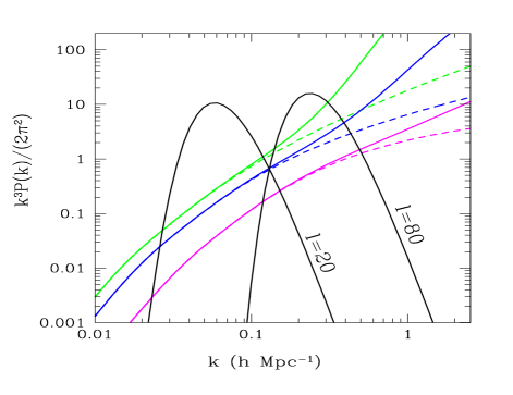
Figure 1: Matter power spectra and ${\cal C}_{l}$ derivatives. From bottom to top at low $l$ are the COBE and cluster consistent predictions for $\Omega_{m}=0.15,0.3,1$, all with $b=1$ (dashed lines show linear theory predictions). The $l=20$ and $l=80$ curves show $k\partial{\cal C}_{l}/\partial{\cal P}_{k}$ for for these two multipole moments (arbitrary normalization).

3.2 The biasing prescription

Although biasing in general is stochastic, non–linear, redshift and scale dependent, we adopt the simplest possible model here in which the galaxy number density fluctuations are directly proportional to the matter density fluctuations. Then we can write $b\equiv\delta_{G}/\delta$, where $\delta=\delta\rho/\bar{\rho}$ is the matter density contrast, $\delta_{G}$ is the galaxy number density contrast, and $b$ is the bias factor.

With this description $P_{G}(k)=b^{2}P(k)$, where $P(k)$ is the matter power spectrum. Note that above we have only calculated the linear theory matter power spectrum. Non-linear corrections are important over the EDSGC range of length scales, and we must incorporate these effects. We derive $P(k)$ from the linear theory power spectra $P_{0}(k)$ by use of a fitting formula (Peacock & Dodds 1996) which provides a good fit to the results of $n$-body calculations. The resulting power spectra are shown by the solid lines in Fig. 1.

We have assumed that the galaxy number density fluctuations are completely determined by the local density contrast. The number density of galaxies must also have some non–local dependence on the density contrast. More complicated modeling of the relationship, or “biasing schemes” (e.g., Cen & Ostriker 1992; Mann, Peacock & Heavens 1998, Dekel & Lahav 1999) are beyond the scope of this paper. In the applications that follow we assume the bias to be independent of time or scale, although our formalism allows inclusion of both of these possibilities.

From analytic theory (e.g., Seljak 2000) we expect the bias to be scale–independent on scales that are larger than any collapsed dark matter halos. Numerical simulations show this to be the case as well (see Blanton et al. 2000; Nayayanan, Berlind & Weinberg 2000) on scales larger than $10h^{-1}$Mpc. Moreover, recent observations by Miller, Nichol & Batuski (2001) show that a scale–independent, linear, biasing model works well when scaling cluster & galaxy data over the range of $200$ to $40h^{-1}$ Mpc. Our results are determined mostly by information from these large scales. Since we find acceptable fits to the data using our constant bias model, we have no evidence for a scale–dependent bias.

3.3 The projection to 2D

As described in the appendix, $C_{l}$ can be calculated from ${\cal P}_{0}(k)$ and the selection function as

$$C_{l}={4\pi}\int{\cal P}_{0}(k)f_{l}(k)^{2}dk/k$$ (12)

where

$$f_{l}(k)\equiv{1\over\bar{G}}\int dz{dr\over dz}j_{l}(kr)r^{2}\bar{g}(z)D(z)bT_{\rm nl}(k,z),$$ (13)

$r$ is the comoving distance along our past light cone, $\bar{g}(z)$ is the mean comoving number density of observable galaxies, $D(z)$ is the growth of perturbations in linear theory relative to $z=0$ and $T_{\rm nl}(k,z)$ is the correction factor for non-linear evolution (Peacock & Dodds 1996).

Equations (12) and (13) are valid for all angular scales. It becomes time–consuming to evaluate the Bessel function on smaller angular scales. Although we always used equations (12) and (13), the reader should know that there is a much more rapid approximation which works well at $l\mathrel{\mathchoice{\lower 3.6pt\vbox{\halign{$\mathsurround=0pt\displaystyle\hfil#\hfil$\cr>\crcr\sim\crcr}}}{\lower 3.6pt\vbox{\halign{$\mathsurround=0pt\textstyle\hfil#\hfil$\cr>\crcr\sim\crcr}}}{\lower 3.6pt\vbox{\halign{$\mathsurround=0pt\scriptstyle\hfil#\hfil$\cr>\crcr\sim\crcr}}}{\lower 3.6pt\vbox{\halign{$\mathsurround=0pt\scriptscriptstyle\hfil#\hfil$\cr>\crcr\sim\crcr}}}}30$:

$$C_{l}={1\over\bar{G}^{2}}\int dz{dr\over dz}P(k=l/r,z)[\bar{g}(z)D(z)bT_{\rm nl}(k=l/r,z)]^{2}.$$ (14)

In order to calculate $C_{l}$, we need to know $\bar{g}(z)$. Since $r^{2}\bar{g}(z)dr/dz=d\bar{G}/dz$ (Baugh & Efstathiou 1993; 1994; our appendix) it is sufficient to know $d\bar{G}/dz$, whose measurement is described in §5.

To give an idea of how $C_{l}$ depends on ${\cal P}(k)$ we plot $k\partial C_{l}/\partial{\cal P}(k)$ in Fig. 1 for $l=20$ and $l=80$. This quantity is the contribution to $C_{l}$ from each logarithmic interval in $k$. Note that it is the breadth of these derivatives that explains the correlations that appear in any attempt to reconstruct $P(k)$ from angular correlation data. The derivatives have some dependence on cosmology; those plotted are for the $\Omega_{m}=0.3$ case.

The angular power spectrum is sensitive not only to the power spectrum today, but to the power spectrum in the past as well. In linear theory, the evolution of the power spectrum is separable in $k$ and $z$; one can write $P(k,z)=P(k,0)D^{2}(z)$ where $D(z)$ is the growth factor well-described by the fitting formula of Carroll, Press & Turner (1992). We also assume that this relation holds for the non-linear power spectra. In truth, non-linear evolution is more rapid at higher $k$ than at lower $k$. We expect our approximation to therefore be overestimates of $C_{l}$, but since we do not use data that reach very far into the non-linear regime, we do not expect this error to be significant.

4 Extraction of Parameters

To find the maximum-likelihood power spectrum, we have iteratively applied the binned version of equation (6). Although equation (6) is used as an iterative means of finding the maximum of the likelihood, it is also convenient to write it as the equivalent equation for ${\cal C}_{B}$, instead of the correction $\delta{\cal C}_{B}$:

$${\cal C}_{B}={1\over 2}\sum_{B^{\prime}}F^{-1}_{BB^{\prime}}{\rm Tr}\left[\left(\Delta\Delta^{\rm T}-N\right)C^{-1}{\partial C\over\partial{\cal C}_{B^{\prime}}}C^{-1}\right],$$ (15)

where the right–hand side is evaluated at the previous iteration value of ${\cal C}_{B}$, ${\cal C}_{B}^{\rm RHS}$, and ${\cal C}_{B}={\cal C}_{B}^{\rm RHS}+\delta{\cal C}_{B}$ is the updated power spectrum.

We have shown how to calculate ${\cal C}_{l}$ from the theoretical parameters. We now need to calculate what ${\cal C}_{B}$ we expect for this ${\cal C}_{l}$. One can show that the expectation value for ${\cal C}_{B}$, given that the data are realized from a power spectrum ${\cal C}_{l}$, is

$$\langle{\cal C}_{B}\rangle = \sum_{l}\sum_{B^{\prime}}F^{-1}_{BB^{\prime}}\sum_{l^{\prime}\in B^{\prime}}F_{ll^{\prime}}{\cal C}_{l}$$ (16)

$$= \sum_{l}{W^{B}_{l}\over l}{\cal C}_{l}$$

where the Fisher matrices on the right-hand side are evaluated at ${\cal C}_{B}^{\rm RHS}$, and the last line serves to define the bandpower window function $W^{B}_{l}$. Note that the sum over $l^{\prime}$ is only from $l_{<}(B^{\prime})$ to $l_{>}(B^{\prime})$. This equation reduces to equation (8) of Knox (1999) in the limit of diagonal $F_{BB^{\prime}}$. It is this expectation value that should be compared to the measured ${\cal C}_{B}$.

As shown by Bond, Jaffe & Knox (2000), the probability distribution of $C_{l}$ is well–approximated by an offset log-normal form. In the sample–variance limit, which applies for our analysis of EDSGC, this reduces to a log–normal distribution. Therefore we take the uncertainty in each ${\cal C}_{B}$ to be log–normally distributed and evaluate the following $\chi^{2}$:

$$\chi^{2}_{\rm EDSGC}(\Omega_{m},b,\sigma_{8}^{c})=$$ (17)

$$\hskip 14.22636pt\sum_{BB^{\prime}}\left(\ln{{\cal C}_{B}}-\ln{{\cal C}_{B}^{t}}\right){\cal C}_{B}F_{BB^{\prime}}{\cal C}_{B^{\prime}}\left(\ln{{\cal C}_{B^{\prime}}}-\ln{{\cal C}_{B^{\prime}}^{t}}\right)$$

$${\cal C}_{B}^{t}\equiv\sum_{l}{W^{B}_{l}\over l}{\cal C}_{l}(\Omega_{m},b,\sigma_{8}^{c})$$ (18)

where $\sigma_{8}=\sigma_{8}^{c}\,\Omega_{m}^{-0.47}$.

Our total $\chi^{2}=\chi^{2}_{\rm EDSGC}+\chi^{2}_{\rm VL}$ includes the contribution from the cluster abundance constraint which is also log-normal:

$$\chi^{2}_{\rm VL}=\left(\ln{\sigma_{8}^{c}}-\ln{0.56}\right)^{2}/\sigma^{2}$$ (19)

where $\sigma={1\over 2}\ln{\left(1+0.32\,\Omega_{m}^{0.24{\rm log}_{10}{\Omega_{m}}}\right)}$ (Viana and Liddle 1996, hereafter VL96). Note that here and throughout we have adopted the more conservative uncertainty in VL96, as opposed to the VL99 uncertainty.

5 Application to the EDSGC

The Edinburgh/Durham Southern Galaxy Catalogue (EDSGC) is a sample of nearly 1.5 million galaxies covering over $1000\ {\rm deg^{2}}$ centered on the South Galactic Pole. The reader is referred to Nichol, Collins & Lumsden (2000) for a full description of the construction of this galaxy catalogue as well as a review of the science derived from this survey. For the EDSGC data, the reader is referred to www.edsgc.org.

For the analysis discussed in this paper, we consider only the contiguous region of the EDSGC defined in Nichol, Collins & Lumsden (2000) and Collins, Nichol & Lumsden (1992) (right ascensions $23<\alpha<3$ hours, through zero hours, and declinations $-42^{\circ}<\delta<-23^{\circ}$). We also restrict the analysis to the magnitude range $10<b_{J}<19.4$. The faint end of this range is nearly one magnitude brighter than the completeness limit of the EDSGC (see Nichol, Collins & Lumsden 2000) but corresponds to the limiting magnitude of the ESO Slice Project (ESP) of Vettolani et al. (1998) which was originally based on the EDSGC. The ESP survey is 85% complete to this limiting magnitude ($b_{j}=19.4$) and consists of 3342 galaxies with redshift determination. This allows us to compute the selection function of the whole EDSGC survey which is shown in Fig. 2. The data shown in this figure has been corrected for the 15% incompleteness in galaxies brighter than $b_{j}=19.4$ with no measured redshifts as well as the mean stellar contamination of 12% found by Zucca et al. (1997) in the EDSGC. These corrections are not strong functions of magnitude; therefore, we apply them as constant values across the whole magnitude range of the survey.

As mentioned above, we need to correct our power spectrum estimates for stellar contamination in the EDSGC map. If the stars are uncorrelated (which we assume) then their presence will suppress the fluctuation power as we now explain. Let $T_{i}$ be the total count in pixel $i$, consisting of galaxies and stars: $T_{i}=G_{i}+S_{i}$ (for simplicity, we consider equal-area pixels). Let $\alpha=0.12$ be the fraction of the total that are stars, so that $\bar{G}=(1-\alpha)\bar{T}$. Then, defining $\Delta_{i}^{G}=(G_{i}-\bar{G})/{\bar{G}}$ and $\Delta_{i}^{S}=(S_{i}-\bar{S})/{\bar{S}}$, we have

$$\Delta_{i} \equiv {T_{i}-\bar{T}\over\bar{T}}$$ (20)

$$= (1-\alpha)\Delta_{i}^{G}+\alpha\Delta_{i}^{S}.$$ (21)

$\Delta_{i}^{G}$ is what we are after: density contrast in the absence of stellar contamination. The second term amounts to a small additional source of noise. Since, as mentioned in §2, the noise is completely unimportant on the scales of interest, we neglect this term. Therefore,

$$\langle\Delta_{i}^{G}\Delta_{j}^{G}\rangle=(1-\alpha)^{-2}\langle\Delta_{i}\Delta_{j}\rangle.$$ (22)

We have accordingly corrected all our ${\cal C}_{B}$ estimates and their error bars upwards by $(1-\alpha)^{-2}\approx 1.29$.

By selection function we mean $d\bar{G}/dz$ where $\bar{G}$ is the mean number of EDSGC galaxies per steradian. The smooth curve in Fig. 2 was chosen to fit the histogram, and is given by

$$\frac{d\bar{G}}{dz}=4\times 10^{5}\exp(-(z/0.06)^{3/2})\left(\frac{z}{0.1}\right)^{3}.$$ (23)

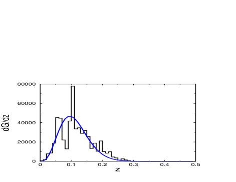
Figure 2: The selection function for the EDSGC; i.e., the mean number of galaxies per steradian per redshift interval.

Restricting ourselves to $b_{J}<19.4$ leaves around 200,000 galaxies. Although this is only $\sim 15\%$ of the total number of galaxies in the EDSGC, the resulting shot noise is still less than the fluctuation power, even at the smallest scales we consider.

We binned the map into 5700 pixels with extent $0.5^{\circ}$ in declination and $0.5^{\circ}$ in right ascension (RA). The pixels are slightly rectangular with varying solid angles; the RA widths correspond to angular distances ranging from $0.46^{\circ}$ at $\delta=-23^{\circ}$ to $0.37^{\circ}$ at $\delta=-42^{\circ}$. This pixelization is fine enough so as not to affect our interpretation of the large–scale fluctuations; it causes a $\sim$4% suppression of the fluctuation power at $l=80$. We have varied the pixelization scale to test this and find that with $1^{\circ}\times 1^{\circ}$ pixels the estimated ${\cal C}_{l}$s change by less than half an error bar for $l<80$.

We also took into account the “drill holes”, locations in the map which were obstructed (e.g. by bright stars). In the case of $0.5^{\circ}\times 0.5^{\circ}$ pixelization about 75 pixels were corrupted by drill holes. Those pixels were assigned large diagonal values in the noise matrix (e.g., Bond, Jaffe & Knox 1998), and thus had negligible weight in the subsequent analysis. The $0.5^{\circ}\times 0.5^{\circ}$ pixelized map is shown in Fig. 3.

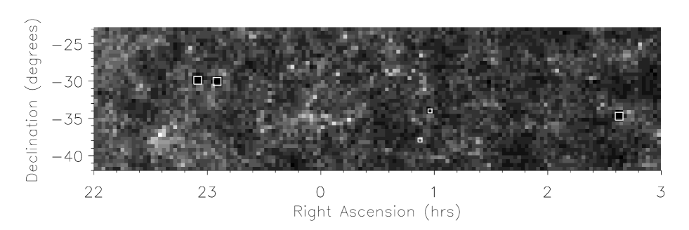
Figure 3: Map of the EDSGC that we used in our analysis ($23<{\rm ra}<3$ hours and $-42<{\rm dec}<-23$ hours, $b_{J}<19.4$). Five of the largest masks are indicated with squares.

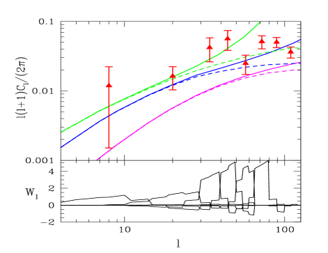
Figure 4: Angular power spectra estimated from the data and predicted for various models. From bottom to top at low $l$ are the COBE and cluster consistent predictions for $\Omega_{m}=0.15,0.3,1$ and $b=1$ (dashed lines show linear theory predictions). The lower panel shows the window functions for the first six bands.

In Fig. 4 we plot the estimated angular power spectrum from the EDSGC data. Also shown in Fig. 4 are our predicted ${\cal C}_{l}$s. For each of these, we can calculate the expected values of ${\cal C}_{B}$ by summing over the window functions, shown in the bottom panel for the six lowest $l$ bands. The jaggedness results from our practice of calculating the Fisher matrix not for every $l$, but for fine bins of $l$ labeled by $b$. We then assume $F_{ll^{\prime}}=F_{bb^{\prime}}/(\delta l(b)\delta l(b^{\prime}))$.

We apply equation (17) with the sum restricted to the six ${\cal C}_{B}$ at lowest $l$. First we keep $\sigma_{8}^{c}$ fixed to the preferred value of 0.56 (VL99) resulting in a $\chi^{2}$ whose contours are shown as the dashed lines in Fig. 5. The minimum of this $\chi^{2}$ is 8.1 for $6-2=4$ degrees of freedom at $\Omega_{m}=0.35$ and $b=1.3$, where $n=0.91$. This is an acceptable $\chi^{2}$; the probability of a larger $\chi^{2}$ is 9%. Moving towards higher $\Omega_{m}$ decreases the VL99 preferred value of $\sigma_{8}$, and thus the preferred value of $b$ increases. Increasing $\Omega_{m}$ also changes the transfer function, requiring a decrease in $n$ in order to agree with both COBE/DMR and cluster abundances. This change in the shape of the angular power spectrum leads to an increase in $\chi^{2}_{\rm EDSGC}$. Moving towards lower $\Omega_{m}$ generates a bluer tilt to the $C_{l}$ shape in two different ways. It leads to higher $n$ for consistency with COBE/DMR and cluster abundances and it also increases the importance of non–linear corrections. These combined effects lead to a rapidly increasing $\chi^{2}_{\rm EDSGC}$ for $\Omega_{m}<0.2$.

The uncertainties on $\sigma_{8}^{c}$ from cluster abundances (as we interpret them) are significantly larger than the EDSGC constraints on $b$ for fixed $\sigma_{8}^{c}$. If we take them into account, we must include additional prior information in order to obtain an interesting constraint on the bias. Since (at fixed $\Omega_{m}$) changing $\sigma_{8}^{c}$ changes $n$, prior constraints on $n$ will help to constrain $\sigma_{8}^{c}$. Therefore we work with the total $\chi^{2}=\chi^{2}_{\rm EDSGC}+\chi^{2}_{VL}+\chi^{2}_{n}$. From a combined analysis of Boomerang-98, Maxima-I and COBE/DMR data, Jaffe et al. (2000) find $n=1\pm 0.1$; hence we adopt $\chi^{2}_{n}=(n-1)^{2}/0.1^{2}$. We marginalize the likelihood, which is proportional to $e^{-\chi^{2}/2}$, over $\sigma_{8}^{c}$.

Figure 5: Contours of constant $\chi^{2}$ in the $\Omega_{m}$ vs. bias plane. The dashed lines are for $\sigma_{8}$ chosen to be at Viana and Liddle maximum-likelihood value. The solid line is the result of marginalizing over $\sigma_{8}$, with the VL99 prior and a prior in $n$ of $1\pm 0.1$. The contour levels show the minimum as well as 2.3 and 6.17 above the minimum, corresponding to 68% and 95.4% confidence levels if the distribution were Gaussian.

Marginalizing over the amplitude constraint from cluster abundances, we find $1.07<b<2.33$ at the best-fit value of $\Omega_{m}=0.35$, and $1.11<b<2.35$ after marginalizing over $\Omega_{m}$ (both ranges 95% confidence). These constraints correspond to the solid and dashed contours respectively in Fig. 5. Figure  6 shows the likelihood of bias, when marginalized either over $\sigma_{8}$ (solid line) or $\Omega_{m}$ (dashed line). Marginalizing over the bias leads to weak constraints on $\Omega_{m}$, unless one insists on allowing only small departures from scale-invariance. With the assumption that the primordial power spectral index is $n=1\pm 0.1$, we find $0.2<\Omega_{m}<0.55$ at 95% confidence. Furthermore, it is interesting that not only do “concordance”–type models, with scale–independent biases provide the best fits to the EDSGC data, but they also provide acceptable fits.

Figure 6: Left panel: likelihood of $b$ marginalized over $\sigma_{8}$ (with $n=1\pm 0.1$ prior) at $\Omega_{m}=0.35$ (solid line), and additionally marginalized over $\Omega_{m}$ (dashed line). Right panel: likelihood of $\Omega_{m}$ with no priors (dotted line), $n$ prior (dashed line), $n$ and our VL priors (solid line).

6 Systematic Errors

In this section we discuss three sources of systematic error: spatially–varying extinction by interstellar dust, deviation of the survey mean from the ensemble mean and deviation from Gaussianity. Above we have assumed their impact on the data to be negligible. In the following we use maps with three different pixelizations: BIGPIX (1.5 deg $\times$ 1.5 deg pixels, a total of $N=650$ of them), MEDPIX (1.0 deg $\times$ 1.0 deg, $N=1425$) and FINEPIX (0.5 deg $\times$ 0.5 deg, $N=5700$). Note that FINEPIX was ultimately used to obtain the cosmological parameter constraints. Coarser pixelizations, however, are easier to work with due to a much smaller number of pixels (in particular, $N\times N$ matrices have to be repeatedly inverted in the quadratic estimator).

6.1 Interstellar Dust

The first possible source of systematic error, interstellar dust, we can dispense with quickly due to the work of Nichol & Collins (1993) and, more recently, Efstathiou & Moody (2000). The former investigated the effects of interstellar dust (using HI and IRAS maps as tracers of the dust) on the observed angular correlation function of EDSGC galaxies (see Collins et al. 1992) and found no significant effect on the angular correlations of these galaxies to $b_{j}=19.5$. We note that Nichol & Collins (1993) also investigated plate–to–plate photometric errors and concluded they were also unlikely to severely effect the angular correlations of EDSGC galaxies. Efstathiou & Moody (2000) used the latest dust maps from Schlegel, Finkbeiner & Davis (1998) to make extinction corrections to the APM catalog and found that for galactic latitudes of $|b|>20^{\circ}$, the corrections have no significant impact on the angular power spectrum. Since all the EDSGC survey area resides at galactic latitudes of $|b|>20^{\circ}$ and has been thoroughly checked for extinction–induced correlations, we conclude that spatially–varying dust extinction has not significantly affected our power–spectrum determinations either.

6.2 Integral Constraint

We are interested in the statistical properties of deviations from the mean surface density of galaxies. This effort is complicated by our uncertain knowledge of the mean. Our best estimate of the ensemble mean is the survey mean. But assuming that the survey mean is equal to the ensemble mean leads to artificially suppressed estimates of the fluctuation power on the largest scales of the survey. This assumption is often referred to as “neglecting the integral constraint” (for discussions, see, e.g., Peacock & Nicholson (1991); Collins, Nichol & Lumsden (1992)).

Let $\bar{G}$ be the ensemble average number of galaxies in a pixel. Let us denote the survey average as

$$\tilde{G}={1\over n_{\rm pix}}\sum_{i}G_{i}.$$ (24)

Since we do not know the ensemble average, in practice we use the survey average to create the contrast map:

$$\tilde{\Delta}_{i}={G_{i}-\tilde{G}\over\tilde{G}}={1\over 1+\epsilon}\left(\Delta_{i}-\epsilon\right)$$ (25)

where

$$\Delta_{i}\equiv{G_{i}-\bar{G}\over\bar{G}}$$ (26)

is the contrast map made with the ensemble average and

$$\epsilon\equiv{\tilde{G}-\bar{G}\over\tilde{G}}$$ (27)

is the fractional difference between the two averages (for simplicity of notation we are assuming equal–area pixels).

Our likelihood function should not have the covariance matrix for $\Delta_{i}$, but instead for $\tilde{\Delta}_{i}$. These are related by

$$\langle\tilde{\Delta}_{i}\tilde{\Delta}_{j}\rangle=\langle\Delta_{i}\Delta_{j}\rangle-\langle\epsilon\left(\Delta_{i}+\Delta_{j}\right)\rangle+\langle\epsilon^{2}\rangle$$ (28)

plus higher order terms. The extra terms of the above equation are easily calculated with the following expressions:

$$\langle\epsilon\Delta_{i}\rangle = {1\over N_{\rm pix}}\sum_{j}\langle\Delta_{i}\Delta_{j}\rangle$$

$$\langle\epsilon^{2}\rangle = {1\over N_{\rm pix}^{2}}\sum_{ij}\langle\Delta_{i}\Delta_{j}\rangle$$ (29)

Each correction term typically contributes 10-20% to the corresponding terms of the covariance matrix (they do not cancel, since there are two linear correction terms; see equation (28)). The main contribution comes from the lowest multipoles, corresponding to largest angles $\theta$. Indeed, the correction terms come almost entirely from our lowest multipole bin. Dropping this bin (or using a $\Lambda$CDM $C_{l}$) reduces the correction terms to 2% or less.

The amplitude of the correction terms can be understood from the weakness of the signal correlations on scales approaching the smaller survey dimension of $19^{\circ}$. In that case, we can write:

$${1\over N_{\rm pix}}\sum_{j}\langle\Delta_{i}\Delta_{j}\rangle\approx 2\pi\int S(\theta)\theta d\theta/\Omega.$$ (30)

where $\Omega$ is the area of the survey, and $S(\theta)$ is the signal covariance, given by the RHS of equation (4) (we have neglected pixel noise). We plot the integrand in Fig. 7 in units of $S(0)$.

Figure 7: The area under the curve is approximately equal to the integral constraint correction terms of equation (28) in units of $S(0)$; see equation (30). The assumed model is $\Omega_{M}=0.3$ with VL99 and COBE/DMR normalization. (The oscillations are due to the fact that only the contributions from multipole moments at $l<180$ were included.)

Fortunately, even though the correction terms are not entirely negligible, their inclusion makes the estimated ${\cal C}_{l}$ change very little. This is shown in Fig. 8. The most significant change is a $\sim 20$% broadening of the error bar of the lowest multipole. Including this effect has a negligible consequence on our cosmological parameter constraints.

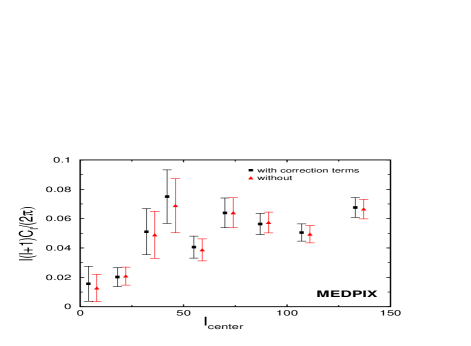
Figure 8: The ${\cal C}_{l}$ determined with and without the integral constraint correction. Shown is the MEDPIX case, and abscissae of points were slightly offset for easier viewing.

6.3 Gaussianity

On large enough scales, we expect the maps to be Gaussian–distributed. Figure  9 shows histograms of the data for the three pixelizations we examined. The histograms are overplotted with the Gaussians with zero mean and variance equal to the pixel variance. One can see the improved consistency with Gaussianity as the pixel size increases.

Figure 9: Histograms of the data, overplotted with Gaussians centered at zero with variances equal to the pixel variances, for maps made with three different pixel sizes. From top to bottom they are: BIGPIX, MEDPIX, FINEPIX.

We applied a Kolmogorov–Smirnov test (e.g., Press et al. 1992) to check for consistency of the above histograms with their corresponding zero–mean Gaussians. We find probabilities that these Gaussians are the parent distributions of $<10^{-10}$, 0.001, and 4.5% for FINEPIX, MEDPIX and BIGPIX respectively, indicating that Gaussianity is a better approximation on large scales than it is on small scales, as expected. We also determined the skewness of the maps in units of the variance to the 1.5 power, and find the same trend of decreasing non–Gaussianity with scale: 1.21, 0.85, 0.79.

The trend with increasing angular scale and the weakness of the $\sim 2\sigma$ discrepancy for the BIGPIX map are reassuring for our analysis that considered only moments $l<80$. Note that a spherical harmonic with $l=80$ has 3 BIGPIX pixels in a wavelength. However, a normalized skewness near unity is worrisome—and this skewness is not decreasing rapidly with increasing angular scale. We discuss possible ways of dealing with this non–Gaussianity in the next section.

7 Discussion

We reduced our sensitivity to the non–Gaussianity of the data by restricting our cosmological parameter analysis to $l<80$. However, the map may still be significantly non–Gaussian even on these large scales. Future analyses of more powerful data sets that result in smaller statistical errors will have to quantify the effects of the Gaussianity assumption, which we have not done here.

The non–Gaussianity may force us towards a Monte–Carlo approach. An analysis procedure similar to the one utilized here may have to be repeated many times on simulated data—where the simulations include the non–linear evolution that presumably is the source of the Gaussianity. The distribution of the recovered parameters can then be used to correct biases and characterize uncertainties.

Monte–Carlo approaches may be necessary for other reasons as well. Recently Szapudi et al. (2000) have tested a quadratic estimator for $C_{l}$ with a simpler (sub–optimal) weighting scheme that only requires on the order of $N^{2}$ operations (or $N\sqrt{N}$ operations using the new algorithms of Moore et al. 2001) instead of $N^{3}$. A drawback is that evaluation of analytic expressions for the uncertainties requires on the order of $N^{4}$ operations. Fortunately, the estimation of $C_{l}$ is rapid enough to permit a Monte–Carlo determination of the uncertainties in a reasonable amount of time.

Note though that Bayesian approaches may still be viable, if it can be shown that non–Gaussian analytic expressions for the likelihood provide an adequate description of the statistical properties of the data. See Magueijo, Hobson & Lasenby (2000) and Contaldi et al. (2000).

To get our constraints on cosmological parameters we fixed the Hubble constant at 70 km/sec/Mpc, or $h=0.7$. We now explain how our bias results and $\Omega_{m}$ results scale for different values of the Hubble constant.

The transfer function depends on the size of the horizon at matter–radiation equality $\lambda_{\rm EQ}$ which is proportional to $1/(\Omega_{m}h^{2})$, or, in convenient distance units of $h^{-1}{\rm Mpc}$, $1/(\Omega_{m}h)$. The latter quantity is the relevant one since all distances come from redshifts and the application of Hubble’s law (in this case the redshifts taken for our selection function) with the result that distances are only known in units of $h^{-1}$Mpc. Thus there is a degeneracy between models with the same value of $\Omega_{m}h$ and different values of $h$.

This degeneracy is broken by the $\Omega_{m}$ dependence of the COBE-normalization of $\delta_{H}$ and the cluster normalization of $\sigma_{8}$. Increasing $h$ at fixed values of $\Omega_{m}h$ means $\Omega_{m}$ decreases, raising both $\delta_{H}$ and $\sigma_{8}$. Ignoring non–linear effects, this can be mimicked by an increase in the bias and only a very slight reddening of the tilt (since $\delta_{H}$ has risen only slightly more than $\sigma_{8}$ and there is a long baseline to exploit).

The end result is that our constraints on $b$ are actually constraints on $b(h/0.7)^{-0.5}$, and our constraints on $\Omega_{m}$ (at least when marginalized over bias) are actually constraints on $\Omega_{m}(h/0.7)$.

8 Conclusions

We have presented a general formalism to analyze galaxy surveys without redshift information. We pixelize the galaxy counts on the sky, and then, using the quadratic estimator algorithm, extract the angular power spectrum – a procedure already in use in CMB data analysis. Just like in the CMB case, one effectively converts complex information contained in the experiment (in this case, locations of several hundred thousand galaxies) into a handful of numbers – the angular power spectrum. One can then use the angular power spectrum for all subsequent analyses.

We apply this method to the EDSGC survey. We compute the angular power spectrum of EDSGC, and combine it with COBE/DMR and cluster constraints to obtain constraints on cosmological parameters. Assuming flat $\Lambda$CDM models with constant bias between galaxies and dark matter, we get $1.11<b<2.35$ and $0.2<\Omega_{m}<0.55$ at 95% confidence.

One advantage of our formalism is that it does not require galaxy redshifts, but only their positions in the sky. This should make it useful for surveys with very large number of galaxies, only a fraction of which will have redshift information. For example, the ongoing SDSS is expected to collect about one million galaxies with redshift information, but also a staggering one hundred million galaxies with photometric information only. Using the techniques presented in this paper, one will be able to convert that information into the angular power spectrum, which can then be used for various further analyses.

A Limber’s Equation

In order to derive the equation giving $C_{l}$ as a function of $P(k)$ we must understand the dependence of the data on the 3D matter density contrast $\delta\equiv\delta\rho/\rho$ as a function of time and space. First, we relate the number of galaxies per unit solid angle $G$ observed from location r in a beam with $FWHM=\sqrt{8\ln{2}}\sigma$ centered on the direction $\hat{\gamma}$ to the comoving number density of detectable galaxies $g$, via

$$G({\hbox{\BF r}},\hat{\gamma})=\int d^{3}r^{\prime}{e^{-|\hat{x}-\hat{\gamma}|^{2}/2\sigma^{2}}\over 2\pi\sigma^{2}}g({\hbox{\BF r}}^{\prime},\tau_{0}-x),$$ (A1)

where ${\hbox{\BF x}}\equiv{\hbox{\BF r}}^{\prime}-{\hbox{\BF r}}$, $x$ is the magnitude of x and $\tau_{0}$ is the conformal distance to the horizon today. To relate $g$ to $\delta$ we simply assume that the galaxies are a biased tracer of the mass, so that $g=\bar{g}(1+b\delta)$. Therefore:

$$\Delta({\hbox{\BF r}},\hat{\gamma}) \equiv {G-\bar{G}\over\bar{G}}$$ (A2)

$$={1\over\bar{G}}\int d^{3}r^{\prime}{e^{-|\hat{x}-\hat{\gamma}|^{2}/2\sigma^{2}}\over 2\pi\sigma^{2}}\bar{g}(x)b(x)\delta({\hbox{\BF r}}^{\prime},\tau_{0}-|x|),$$

where we have allowed for a time-dependent (and therefore $x$-dependent) bias. If we further assume that the density contrast grows uniformly with time, with growth factor $D(x)$, then we can write:

$$\Delta({\hbox{\BF r}},\hat{\gamma})={1\over\bar{G}}\int d^{3}r^{\prime}{e^{-|\hat{x}-\hat{\gamma}|^{2}/2\sigma^{2}}\over 2\pi\sigma^{2}}\bar{g}(x)b(x)\delta({\hbox{\BF r}}^{\prime},\tau_{0})D(x).$$ (A3)

Calculating $w(\theta_{12})=\langle\Delta({\hbox{\BF r}},\hat{\gamma}_{1})\Delta({\hbox{\BF r}},\hat{\gamma}_{2})\rangle$ and then taking its Legendre transform yields (after a fair amount of algebra):

$$C_{l}={2\over\pi}\int k^{2}dkP(k)f_{l}(k)^{2}$$ (A4)

where

$$f_{l}(k)\equiv{1\over\bar{G}}\int{dx\over F(x)}j_{l}(kx)x^{2}\bar{g}(x)D(x)b(x)$$ (A5)

and $F(x)$ enters the metric via

$$ds^{2}=a^{2}\left[d\tau^{2}-dx^{2}/F(x)+x^{2}d\theta^{2}+x^{2}\sin^{2}\theta d\phi^{2}\right].$$ (A6)

For zero mean curvature $F(x)=1$; expressions valid for general values of the curvature are given by Peebles (1980, equation (50.16)).

Note that

$$\bar{G} = \int{r^{2}\over F(r)}\bar{g}(r)dr$$ (A7)

$$= \int dz{d\bar{G}\over dz}$$

and therefore

$${r^{2}\over F(r)}\bar{g}(r)dr/dz={d\bar{G}\over dz}.$$ (A8)

One can use equations (A4) and (A5) to calculate the expected value of $C_{l}$ for any theory. The only information one needs from the survey to do this is $\bar{g}(r)$ or ${d\bar{G}/dz}$. The latter is preferable, and what we use in our application, because it is directly observable as long as redshifts in some region are available.

References

- Balbi et al. (2000) Balbi, S., et al. 2000, ApJL, 545, 1
- Baugh & Efstathiou (1993) Baugh, C. M., & Efstathiou, G 1993, MNRAS, 265, 145
- Baugh & Efstathiou (1994) Baugh, C. M., & Efstathiou, G 1994, MNRAS, 267, 323
- Blanton et al. (2000) Blanton, M. et al. 2000, ApJ, 531, 1
- Bond, Jaffe & Knox (1998) Bond, J. R., Jaffe, A. H., & Knox, L. 1998, Phys. Rev. D, 57, 2117
- Bond, Jaffe & Knox (2000) Bond, J. R., Jaffe, A. H., & Knox, L. 2000, ApJ, 533, 19
- Bunn & White (1995) Bunn, E., & White, M., 1995, ApJ, 450, 477
- Burles, Nollett & Turner (2000) Burles, S., Nollett, K., & Turner, M. S. 2000, ApJL, submitted (astro-ph/00010171)
- Burles & Tytler (1998) Burles, S., & Tytler, D. R. 1998, ApJ, 499, 699
- Carroll, Press & Turner (1992) Carroll, S. M., Press, W. H., & Turner, E. L. 1992, Ann.Rev.Astron.Astrophys., 30, 499
- Cen & Ostriker (1992) Cen, R., & Ostriker, J. P. 1992, 399, L113
- Collins, Nichol & Lumsden (1992) Collins, C. A., Nichol, R. C., & Lumsden, S. L. 1992, MNRAS, 154, 295
- Contaldi et al. (2000) Contaldi, C., Ferreira, P., Magueijo, J., & Gorski, K. 2000, ApJ, 534, 25
- de Bernardis et al. (2000) de Bernardis, P., et al. 2000, Nature, 404, 955
- (15) Dekel, A., & Lahav, O. 1999, ApJ, 520, 24
- Dodelson & Gaztañaga (2000) Dodelson, S., & Gaztanaga, E. 2000, MNRAS, 312, 774
- (17) Efstathiou, G. & Moody, S.J. 2000 (astro-ph/0010478)
- Eisenstein & Hu (1999) Eisenstein, D. J., & Hu, W 1999, ApJ, 511, 5
- Eisenstein & Zaldarriaga (1999) Eisenstein, D. J., & Zaldarriaga, M., ApJ, submitted (astro-ph/9912149)
- Gaztañaga & Baugh (1998) Gaztanaga, E., & Baugh, C. M. 1998, MNRAS, 294, 229
- Gaztañaga & Hui (1999) Gaztañaga, E., & Hui, L., ApJ, 519, 622
- Groth & Peebles (1977) Groth, E. J., & Peebles, P. J. E. 1977, ApJ, 217, 385
- Hanany et al. (2000) Hanany, S., et al. 2000, ApJL, 545, 5
- Hivon et al. (1995) Hivon, E., Bouchet, F.R., Colombi, S., & Juszkiewicz, R. 1995, A& A, 298, 643
- Jaffe et al. (2000) Jaffe, A. H. et al. 2000, Phys. Rev. Lett., submitted (astro-ph/0007333)
- Knox (1999) Knox, L. 1999, Phys. Rev. D, 60, 103516
- Knox et al. (1998) Knox, L., Bond, J.R., Jaffe, A.H., Segal, M. and Charbonneau, D. 1998, Phys. Rev. D, 58, 083004
- Lange et al. (2000) Lange, A. E, et al. 2000, Phys. Rev. D submitted (astro-ph/0005004)
- Limber (1953) Limber, D. N. 1953, ApJ 117, 134
- Lucy (1974) Lucy, L. B. 1974, AJ, 79, 745
- Maddox et. al. (1990) Maddox, S. J., Efstathiou, G. Sutherland, W. J., & Loveday J. 1990, MNRAS 242, 43P
- Mann, Peacock & Heavens (1998) Mann, R.G., Peacock, J. A., & Heavens, A. F. 1998, MNRAS, 293, 209
- (33) Miller, C.J., Nichol, R.C., & Batuski, D., 2001, ApJ, submitted
- (34) Moore, A., et al., 2000, Proceedings of MPA/MPE/ESO Conference ”Mining the Sky”, see astroph/0012333
- (35) Nichol, R.C., & Collins, C.A., 1993, MNRAS, 265, 867
- (36) Nichol, R.C., Collins, C.A., & Lumsden, S.L., 2000, ApJS, submitted (astro-ph/0008184)
- Peacock & Dodds (1996) Peacock, J. A., & Dodds, S. J. 1996, MNRAS, 280, L19
- Peacock & Nicholson (1991) Peacock, J. A., & Nicholson, D. 1991, MNRAS, 253, 307
- Peebles (1980) Peebles, P. J. E. 1980, The Large-Scale Structure of the Universe (Princeton Univ. Press)
- Peebles & Hauser (1974) Peebles, P. J. E., & Hauser, M. G. 1974, ApJS, 28, 19
- Pierpaoli & al. (2000) Pierpaoli, E., Scott, D., & White, M. 2000, MNRAS, submitted (astro-ph/0010039)
- Press et al. (1992) Press, W. H., Teukolsky, S. A., Vetterling, W. T., & Flannery, B. P. 1992, Numerical Recipes in C (Cambridge Univ. Press)
- Rocha et al. (2000) Rocha, G., Magueijo, J., Hobson, M., & Lasenby, A. 2000, MNRAS, submitted (astro-ph/0008070)
- Schlegel et al. (1998) Schlegel, D.J., Finkbeiner, D. P., & Davis, M., 1998, ApJ 500, 525
- Seljak (2000) Seljak, U., 2000, MNRAS, 318, 203
- Seljak & Zaldarriaga (1996) Seljak, U., & Zaldarriaga, M. 1996, ApJ, 469, 437
- Szapudi et al. (2000) Szapudi, I., et al. 2000, ApJL, submitted (astro-ph/0010256)
- Tegmark (1997) Tegmark, M. 1997, Phys. Rev. D, 55, 5895
- Tegmark et al. (1998) Tegmark, M., Hamilton, A. J. S., Strauss, M. A., Vogeley, M. S., & Szalay, A. S. 1998, ApJ, 499, 555
- Vettolani et al. (1998) Vettolani, G. et al. 1998, A&AS, 130, 323
- Viana & Liddle (1996) Viana, P. T. P., & Liddle, A. R., 1996, MNRAS, 281, 323.
- Viana & Liddle (1999) Viana, P. T. P., & Liddle, A. R., 1999, MNRAS, 303, 535.
- York et al. (2000) York, D.G., et al. (The SDSS Collaboration) 2000, AJ, 120, 1579
- Zucca et al. (1997) Zucca, E. et al. 1997, A&A, 326, 477