The Formal Underpinnings of the Response Functions used in X-Ray Spectral Analysis

Abstract

This work provides an in-depth mathematical description of the response functions that are used for spatial and spectral analysis of X-ray data. The use of such functions is well-known to anyone familiar with the analysis of X-ray data where they may be identified with the quantities contained in the Ancillary Response File (ARF), the Redistribution Matrix File (RMF), and the Exposure Map. Starting from first-principles, explicit mathematical expressions for these functions, for both imaging and dispersive modes, are arrived at in terms of the underlying instrumental characteristics of the telescope including the effects of pointing motion. The response functions are presented in the context of integral equations relating the expected detector count rate to the source spectrum incident upon the telescope. Their application to the analysis of several source distributions is considered. These include multiple, possibly overlapping, and spectrally distinct point sources, as well as extended sources. Assumptions and limitations behind the usage of these functions, as well as their practical computation are addressed.

1 Introduction

It is a basic tenet of X-ray spectral analysis that the source flux incident at the telescope is related to the observed count rate through an integral equation involving the effective area of the telescope. The most commonly accepted technique for dealing with this equation involves the use of spectral analysis programs such as xspec (Arnaud, 1996). The effective area is input into these programs via a file called the Ancillary Response File, or ARF. In addition, the energy resolution of the detector is specified by the Redistribution Matrix File, or RMF. This work presents formal descriptions of the quantities embodied by the ARF and RMF in terms of the underlying instrumental responses, making a clear connection between the incident source flux and the observed count rate.

Roughly speaking, the effective area of an X-ray telescope composed of a mirror and a detector is more or less the product of the effective area of the mirror with the quantum efficiency (QE) of the detector. However, the ARF, which relates observed counts to a source flux, also depends upon observation-dependent quantities such as the detailed aspect history of the telescope, its point spread function (PSF), and upon details of the analysis itself, e.g., the filtering and binning of the observed data.

With the advent of the Chandra X-ray Observatory (CXC, 2000), all of the subtleties introduced by the shape of the PSF and the telescope aspect motion were deemed important for the computation of an ARF. Chandra is well calibrated (Weisskopf et al., 2000) and, with its unprecedented combined spectral and spatial response, a precise definition of the ARF that incorporates the effects of spacecraft motion and the PSF is necessary in order to perform spectral analysis at the highest resolution of the instrument.

The main goal of this work is to present an explicit first-principles derivation of the ARF by including the proper treatment of telescope motion (e.g., dither) and the PSF, as well as any filtering of the data. The bottom-up approach taken here necessarily implies that a meaningful and consistent derivation can be achieved by considering the role of the ARF in spectral analysis. As a result, the ARF is presented in the context of integral equations that connect the incident X-ray flux to an expected count rate.

Traditionally, the ARF and RMF have been used primarily for the analysis of spectral image data. An important aspect of this work is to extend this approach to the analysis of dispersive spectral data, such as data obtained by Chandra or Newton. To this end, definitions of an ARF and an RMF are presented that are suitable for dispersive data analysis, and which may be utilized by existing spectral analysis software.

One of the original motivations for this work was the need to create a related object, an exposure map, for use in the analysis of data obtained by the Chandra X-ray Observatory. This paper also gives a rigorous definition of the exposure map and discusses some of its uses and its limitations in spectral image analysis. The resulting definition is consistent with current use, intuition, and physics.

The next section contains a discussion of the general response of an X-ray telescope and also serves to introduce the notation and conventions used throughout this paper. Although originally inspired by the need to create ARFs and exposure maps for Chandra, the presentation has been kept as general as possible without focusing on any particular telescope or instrument. A derivation of the imaging ARF follows in section 3 where its application to several problems is considered. These include the problem of multiple overlapping point sources. Section 4 contains a definition of the exposure map and explores its use as well as its limitations in dealing with extended sources. The definition of a dispersive ARF and RMF that are suitable for use in the analysis of dispersive spectral data are given in section 5. Following the summary of the paper is an appendix that considers the practical computation of these objects.

2 Telescope Response

Let $S(\lambda,\mbox{\boldmath$\hat{p}$})d{\lambda}\;\mbox{\bf d}\mbox{\boldmath$\hat{p}$}$ represent the number of photons per unit area per unit time incident upon the telescope with directions that lie in the cone of directions between $\hat{p}$ and $\mbox{\boldmath$\hat{p}$}+\mbox{\bf d}\mbox{\boldmath$\hat{p}$}$, and whose wavelengths lie between $\lambda$ and $\lambda+d{\lambda}$. This source flux is assumed to be time-independent. Similarly, let $S_{D}(h,\sigma,t)\mbox{d}{\sigma}$ represent the expected number of counts per unit time, in pulse-height bin $h$, within a region of area $\mbox{d}{\sigma}$ at the position $\sigma$ on the detector. (Although in this paper, $h$ is a discrete quantity that represents a pulse-height channel, one could easily generalize $h$ to a continuous quantity such as a voltage by introducing the infinitesimal $\mbox{d}{h}$ and replacing $\sum_{h}$ by $\int\mbox{d}{h}$.)

In general, the count rate will be time-dependent even if the source flux does not vary with time. This time-dependence arises from several effects, including but not limited to telescope pointing motion (e.g., pointing wobble or dither), detector electronics, telemetry saturation, and thermal expansion effects that cause the movement of individual telescope subsystems with respect to one another.

As used here, pointing is the measured, generally periodic movement of a coordinate system attached to the optical axis with respect to a coordinate system fixed with respect to the sky. These two coordinate systems are related by a time-dependent rotation matrix ${\cal R}(t)$ which completely characterizes the pointing. It is assumed that complete knowledge of ${\cal R}(t)$ is available from, e.g., an on-board aspect system, at some level of accuracy (see section 2).

In the coordinate system fixed with respect to optical axis, the source flux will appear to be time-dependent according to

$$S(\lambda,\mbox{\boldmath$\hat{p}$},t)=S(\lambda,{\cal R}^{-1}(t)\cdot\mbox{\boldmath$\hat{p}$}).$$ (1)

This equation simply expresses the fact that an observer fixed to the telescope will see a time dependent source and that this induced time dependence is a direct consequence of telescope motion. In the telescope coordinate system, the source flux and the count rate are related to one another via the equation

$$S_{D}(h,\sigma,t)=\int\mbox{d}\lambda\int\mbox{\bf d}\mbox{\boldmath$\hat{p}$}\;R_{T}(h,\lambda,\sigma,\mbox{\boldmath$\hat{p}$},t)S(\lambda,{\cal R}^{-1}(t)\cdot\mbox{\boldmath$\hat{p}$}),$$ (2)

which defines the total response $R_{T}(h,\lambda,\sigma,\mbox{\boldmath$\hat{p}$},t)$ of the telescope. It is an extremely complicated function that incorporates all elements of the telescope such as the detector and its electronics, the mirror, and diffraction gratings, if present. Since the units of $S_{D}(h,\sigma,t)$ are counts per unit detector area per unit time, and the units of $S(\lambda,\mbox{\boldmath$\hat{p}$})\mbox{d}{\lambda}$ are photons per unit aperture area per unit time, it follows that the response $R_{T}(h,\lambda,\sigma,\mbox{\boldmath$\hat{p}$},t)$ is a unitless quantity (counts/photon $\times$ aperture area/detector area).

The mathematical form of equation (2) represents a linear mapping from $S$ to $S_{D}$. Hence, strictly speaking, equation (2) is valid only when one can neglect non-linear effects such as local gain depression or pile-up, i.e., a non-linear effect caused by the finite time resolution of the detector. Pile-up can be treated, at least in principle, by making the response $R_{T}(h,\lambda,\sigma,\mbox{\boldmath$\hat{p}$},t)$ a function of the incident flux $S(\lambda,\mbox{\boldmath$\hat{p}$})$. However, this topic is beyond the scope of the present work and will be addressed elsewhere (Davis, 2000).

The explicit time-dependence of $R_{T}(h,\lambda,\sigma,\mbox{\boldmath$\hat{p}$},t)$ is due to effects associated with telemetry saturation, thermal expansion, and so on. It is assumed that all but the time-dependence associated with internal movement of the telescope subsystems may be encapsulated in a function $T(\sigma,t)$ that factors out of $R_{T}(h,\lambda,\sigma,\mbox{\boldmath$\hat{p}$},t)$, i.e.,

$$R_{T}(h,\sigma,\lambda,\mbox{\boldmath$\hat{p}$},t)=T(\sigma,t)R(h,\sigma,\lambda,\mbox{\boldmath$\hat{p}$},t).$$ (3)

In this equation the residual time-dependence of the response function $R(h,\sigma,\lambda,\mbox{\boldmath$\hat{p}$},t)$ depends only upon the relative movements of the individual telescope subsystems. The function $T(\sigma,t)$ can be thought of as representing the the so-called “good-time intervals”, or GTIs. However, $T(\sigma,t)$ could play a more general role than this because it could include the effects of bad-pixels, which themselves may be time-dependent, as well as any dead-time factors associated with telemetry saturation. It should also be noted that although the incident source flux has been assumed to be independent of time, $T(\sigma,t)$ could encompass time-dependent variations in the source flux as long as the spectral shape itself does not depend upon time. In this case, only the amplitude of the flux is time-dependent and this time-dependence may be factored out of the incident source flux and into the function $T(\sigma,t)$. Further exploration of this possibility is left to the reader. Suffice it to say that the actual values that $T(\sigma,t)$ take on are not important in what follows. Hence, equation (2) can be written

$$S_{D}(h,\sigma,t) = T(\sigma,t)\int\mbox{d}\lambda\int\mbox{\bf d}\mbox{\boldmath$\hat{p}$}\;R(h,\sigma,\lambda,\mbox{\boldmath$\hat{p}$},t)S(\lambda,{\cal R}^{-1}(t)\cdot\mbox{\boldmath$\hat{p}$})$$

$$= T(\sigma,t)\int\mbox{d}\lambda\int\mbox{\bf d}\mbox{\boldmath$\hat{p}$}\;R(h,\sigma,\lambda,{\cal R}(t)\cdot\mbox{\boldmath$\hat{p}$},t)S(\lambda,\mbox{\boldmath$\hat{p}$}),$$

where the last form follows from the change of variables $\mbox{\boldmath$\hat{p}$}\longrightarrow{\cal R}(t)\cdot\mbox{\boldmath$\hat{p}$}$ and noting that because the matrix ${\cal R}(t)$ is orthogonal, the Jacobian of the transformation is unity.

Assuming that the response depends upon several independent telescope subsystems, it may be factored it into subsystem-dependent pieces. The specific form of the factorization will depend upon the actual physical relationships between the various subsystems. For a prototypical X-ray telescope with a focusing mirror at the aperture of the telescope that focuses X-rays onto a position-sensitive detector, an appropriate factorization is given by

$$R(h,\sigma,\lambda,\mbox{\boldmath$\hat{p}$},t)=D(h,\sigma,\lambda)\int\mbox{\bf d}\mbox{\boldmath$\hat{p}$}^{\prime}\;\delta(\sigma-\sigma(\mbox{\boldmath$\hat{p}$}^{\prime},t)){\cal F}(\lambda,\mbox{\boldmath$\hat{p}$}^{\prime},\mbox{\boldmath$\hat{p}$})M(\lambda,\mbox{\boldmath$\hat{p}$}).$$ (5)

A different factorization may have to be use to describe the response of some other type of telescope (see section 5 for the factorization needed to to describe the presence of a diffraction grating). In this equation, $M(\lambda,\mbox{\boldmath$\hat{p}$})$ is the off-axis effective area of the mirror, and $D(h,\sigma,\lambda)$ represents the probability that a photon with wavelength $\lambda$ at position $\sigma$ on the detector will give rise to a pulse-height $h$. The term involving the delta function symbolizes the passage of a photon with direction $\mbox{\boldmath$\hat{p}$}^{\prime}$ from the mirror to the position $\sigma$ on the detector via the coordinate transformation $\sigma(\mbox{\boldmath$\hat{p}$}^{\prime},t)$. In general, this function is time-dependent and represents any relative motion that exists between the mirror and the detector.

The PSF (Point Spread Function) of the telescope is represented by the function ${\cal F}(\lambda,\mbox{\boldmath$\hat{p}$}^{\prime},\mbox{\boldmath$\hat{p}$})$, which is assumed to satisy the normalization condition

$$1=\int\mbox{\bf d}\mbox{\boldmath$\hat{p}$}^{\prime}{\cal F}(\lambda,\mbox{\boldmath$\hat{p}$}^{\prime},\mbox{\boldmath$\hat{p}$}).$$ (6)

Its definition is based upon the idea (see figure 1) that the mirror itself (e.g., one of a typical type-I Wolter design) may be modeled by the appropriate probability distribution for photons to enter and leave the mirror at a single point (the so-called “mirror node”), with an effective area given by $M(\lambda,\mbox{\boldmath$\hat{p}$})$. As indicated in figure 1, the PSF defined in this way will also depend (implicitly) upon the position of the detector and its relationship to the focal surface. For simplicity, in the following it will be assumed that the variations in the movement of the detector with respect to the mirror during the course of an observation are small enough that the PSF may be regarded as independent of time to sufficient accuracy. The reader should note that a perfect PSF defined in this sense is represented by

$${\cal F}_{\mbox{\tiny perfect}}(\lambda,\mbox{\boldmath$\hat{p}$}^{\prime},\mbox{\boldmath$\hat{p}$})=\delta(\mbox{\boldmath$\hat{p}$}^{\prime}-\mbox{\boldmath$\hat{p}$}).$$ (7)

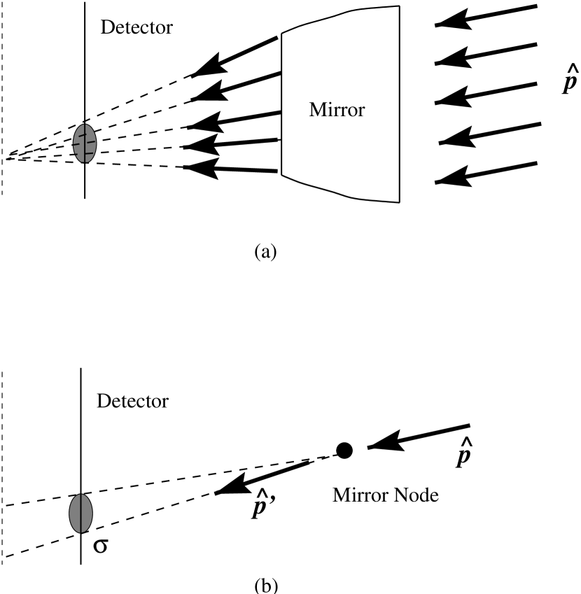
Figure 1: Figure illustrating how the PSF function ${\cal F}(\lambda,\mbox{\boldmath$\hat{p}$}^{\prime},\mbox{\boldmath$\hat{p}$})$ may be used to accurately model a realistic mirror of finite extent. The top portion of the figure shows a “realistic” mirror with the detector in a de-focused position. In this position photons from a distant point source enter the mirror at the front and exit the mirror at the back, and are focused towards a point behind the detector causing the point source to appear out of focus. The bottom part of the figure shows that this effect can be modeled in terms of the concept of a “mirror node”, where rays enter and leave the same point with the appropriate redistribution ${\cal F}(\lambda,\mbox{\boldmath$\hat{p}$}^{\prime},\mbox{\boldmath$\hat{p}$})$ of “incoming” photons with direction $\hat{p}$ into “outgoing” ones with direction $\mbox{\boldmath$\hat{p}$}^{\prime}$. In particular, note that the same PSF function appropriate for the de-focused position of the detector cannot be used to model the image when the detector is at the focal position; there a different PSF will be required. In other words, for ${\cal F}(\lambda,\mbox{\boldmath$\hat{p}$}^{\prime}.\mbox{\boldmath$\hat{p}$})$ to accurately model the mirror, it also depends implicitly upon the location of the detector with respect to the focal surface.

Generally speaking, the detector response $D(h,\sigma,\lambda)$ can be factored into a QE (Quantum Efficiency) $Q(\sigma,\lambda)$ and a redistribution function $D_{R}(h,\sigma,\lambda)$:

$$D(h,\sigma,\lambda)=D_{R}(h,\sigma,\lambda)Q(\sigma,\lambda).$$ (8)

The function $D_{R}(h,\sigma,\lambda)$ is known as the redistribution matrix function, or RMF (George et al., 2000), and represents a mapping, or redistribution, from wavelength to pulse-height by the detector. Without any loss of generality, it is assumed to be normalized to unity via

$$1=\sum_{h}D_{R}(h,\sigma,\lambda).$$ (9)

Alternatively, the quantum efficiency may be defined by

$$Q(\sigma,\lambda)=\sum_{h}D(h,\sigma,\lambda).$$ (10)

In general, as indicated here the RMF varies with position on the detector, although many applications assume a spatially constant RMF. In contrast, the quantum efficiency function $Q(\sigma,\lambda)$ is assumed to contain the effects of (static) bad pixels, detector dead regions, detector boundaries, and so on, all of which cause it to vary spatially.

Using the response function given by equation (5), the expected count rate from the source $S(\lambda,\mbox{\boldmath$\hat{p}$})$ is seen to be

$$S_{D}(h,\sigma,t) = T(\sigma,t)\int\mbox{d}\lambda\int\mbox{\bf d}\mbox{\boldmath$\hat{p}$}\;R(h,\sigma,\lambda,\mbox{\boldmath$\hat{p}$}_{t},t)S(\lambda,\mbox{\boldmath$\hat{p}$})$$

$$= T(\sigma,t)\int\mbox{d}\lambda\;D(h,\sigma,\lambda)\int\mbox{\bf d}\mbox{\boldmath$\hat{p}$}^{\prime}\;\delta(\sigma-\sigma(\mbox{\boldmath$\hat{p}$}^{\prime},t))\int\mbox{\bf d}\mbox{\boldmath$\hat{p}$}\;{\cal F}(\lambda,\mbox{\boldmath$\hat{p}$}^{\prime},\mbox{\boldmath$\hat{p}$}_{t})M(\lambda,\mbox{\boldmath$\hat{p}$}_{t})S(\lambda,\mbox{\boldmath$\hat{p}$}),$$

where, for notational simplicity, $\mbox{\boldmath$\hat{p}$}_{t}$ symbolizes ${\cal R}(t)\cdot\mbox{\boldmath$\hat{p}$}$.

Telescope pointing motion will cause events to appear spatially mixed together when expressed as an image in detector coordinates. For this reason, it is preferable to work in the sky coordinate system where one can remove the effects of the motion by projecting the events to the sky in the appropriate manner. Thus, we define an aspect-corrected count rate via

$$S_{A}(h,\mbox{\boldmath$\hat{p}$},t)=J(\sigma(\mbox{\boldmath$\hat{p}$}_{t},t),\mbox{\boldmath$\hat{p}$}_{t},t)S_{D}(h,\sigma(\mbox{\boldmath$\hat{p}$}_{t},t),t),$$ (12)

where $J(\sigma,\mbox{\boldmath$\hat{p}$},t)$ is the instantaneous Jacobian of the transformation from the detector coordinate $\sigma$ to the sky coordinate $\hat{p}$ via the inversion of $\sigma(\mbox{\boldmath$\hat{p}$}_{t},t)$. Physically, the Jacobian represents the stretching or magnification of an element of area on the detector as it appears in the sky.

By making use of the well known change of variable formula for delta functions expressed in the form

$$\delta(\sigma(\mbox{\boldmath$\hat{p}$}_{t},t)-\sigma(\mbox{\boldmath$\hat{p}$}^{\prime},t))=\frac{\delta(\mbox{\boldmath$\hat{p}$}^{\prime}-\mbox{\boldmath$\hat{p}$}_{t})}{J(\sigma(\mbox{\boldmath$\hat{p}$}_{t},t),\mbox{\boldmath$\hat{p}$}_{t},t)},$$ (13)

one can show that the aspect-corrected count rate is

$$S_{A}(h,\mbox{\boldmath$\hat{p}$}^{\prime},t)=T(\sigma(\mbox{\boldmath$\hat{p}$}^{\prime}_{t},t),t)\int\mbox{d}\lambda\;D(\sigma(\mbox{\boldmath$\hat{p}$}^{\prime}_{t},t),h,\lambda)\int\mbox{\bf d}\mbox{\boldmath$\hat{p}$}\;{\cal F}(\lambda,\mbox{\boldmath$\hat{p}$}^{\prime}_{t},\mbox{\boldmath$\hat{p}$}_{t})M(\lambda,\mbox{\boldmath$\hat{p}$}_{t})S(\lambda,\mbox{\boldmath$\hat{p}$}).$$ (14)

The above equation assumes that complete knowledge of the aspect history is available in order to perform the aspect correction. In general, there will be uncertainties in the aspect solution which in turn leads to spatial uncertainties in the aspect corrected count rate. Mathematically, this will manifest itself as a broadening or smearing of the delta function in equation (13) by an amount that depends upon the aspect uncertainties. The most straightforward way to handle this effect is to absorb the uncertainties into the PSF itself. For this reason, in the following ${\cal F}_{A}(\lambda,\mbox{\boldmath$\hat{p}$}^{\prime},\mbox{\boldmath$\hat{p}$})$ will denote the PSF that includes the effect of the aspect uncertainties.

3 Derivation of the ARF

The total number of expected counts with pulse-height $h$ over an observation interval $\tau$ in some region $\Omega$ can be computed by integrating $t$ over the observation interval and $\mbox{\boldmath$\hat{p}$}^{\prime}$ over the sky region $\Omega$, i.e.,

$$C_{\Omega}(h) = \int_{\Omega}\mbox{\bf d}\mbox{\boldmath$\hat{p}$}^{\prime}\int_{0}^{\tau}\mbox{d}{t}\;S_{A}(h,\mbox{\boldmath$\hat{p}$}^{\prime},t)$$

$$= \int\mbox{d}\lambda\int_{\Omega}\mbox{\bf d}\mbox{\boldmath$\hat{p}$}^{\prime}\int_{0}^{\tau}\mbox{d}{t}\;T(\sigma(\mbox{\boldmath$\hat{p}$}^{\prime}_{t},t),t)D(\sigma(\mbox{\boldmath$\hat{p}$}^{\prime}_{t},t),h,\lambda){\cal F}_{A}(\lambda,\mbox{\boldmath$\hat{p}$}^{\prime}_{t},\mbox{\boldmath$\hat{q}$}_{t})M(\lambda,\mbox{\boldmath$\hat{q}$}_{t})S(\lambda,\mbox{\boldmath$\hat{p}$}).$$

By using equation (8) and assuming for the moment that the RMF does not vary with position, the previous equation can be rewritten as

$$C_{\Omega}(h)=\tau_{\mbox{\tiny eff}}\int\mbox{d}\lambda\;D_{R}(h,\lambda)\int\mbox{\bf d}\mbox{\boldmath$\hat{p}$}\;A_{\Omega}(\lambda,\mbox{\boldmath$\hat{p}$})S(\lambda,\mbox{\boldmath$\hat{p}$}),$$ (16)

where

$$A_{\Omega}(\lambda,\mbox{\boldmath$\hat{p}$})=\frac{1}{\tau_{\mbox{\tiny eff}}}\int_{\Omega}\mbox{\bf d}\mbox{\boldmath$\hat{p}$}^{\prime}\int_{0}^{\tau}\mbox{d}{t}\;T(t)Q(\lambda,\sigma(\mbox{\boldmath$\hat{p}$}^{\prime}_{t},t)){\cal F}_{A}(\lambda,\mbox{\boldmath$\hat{p}$}^{\prime}_{t},\mbox{\boldmath$\hat{p}$}_{t})M(\lambda,\mbox{\boldmath$\hat{p}$}_{t})$$ (17)

and the effective exposure time is given by

$$\tau_{\mbox{\tiny eff}}=\int_{0}^{\tau}\mbox{d}{t}\;T(t).$$ (18)

For simplicity it has been assumed that the good-time interval function $T(t)$ does not depend upon detector position.

Equation 17 defines the ARF. It has the units of area $\times$ counts per photon and depends upon the region $\Omega$, wavelength $\lambda$, and sky position $\hat{p}$. However, for the purposes of point-source analysis, knowledge of the ARF is required only at the position of the point source, where it may be regarded as depending only upon wavelength with the understanding that it is valid only for that source position and region. But for arbitrary sources, it should be regarded as an explicit function of $\hat{p}$.

Armed with the ARF, equation (16) is an integral equation that may be “solved” to yield the source distribution $S(\lambda,\mbox{\boldmath$\hat{p}$})$ from the observed aspect-corrected counts $C_{\Omega}(h)$. Actually, because of the integration over the sky region $\Omega$, much of the spatial dependence in $S(\lambda,\mbox{\boldmath$\hat{p}$})$ will be lost and in practice one will have to assume a known spatial dependence; the examples below illustrate this point more fully. One should also realize that the kernel of equation (16) is really a probability distribution and that the observed number of counts will most likely differ from the expected number of counts predicted by the equation. This implies that equation (16) does not really have a unique solution (for a finite observation time), and any method of “solving” should allow for fluctuations in the number of counts. One must also take into account any external background sources as well as any internal background produced by, say, noise in the detector. Techniques for treating this equation are beyond the scope of this paper and may be found elsewhere (Arnaud, 1996; Kahn and Blissett, 1980).

In the next few sections, equation (16) is considered in the context of various source distributions. The problem of the practical computation of the ARF is taken up in the appendix.

3.1 A Single Point Source

A point source located at position $\hat{q}$ in the sky with a spectrum $s(\lambda)$ may be represented using the source distribution

$$S(\lambda,\mbox{\boldmath$\hat{p}$})=s(\lambda)\delta(\mbox{\boldmath$\hat{p}$}-\mbox{\boldmath$\hat{q}$}).$$ (19)

Substituting this equation into equation (16) yields

$$C_{\Omega}(h)=\tau_{\mbox{\tiny eff}}\int\mbox{d}\lambda\;D_{R}(h,\lambda)A_{\Omega}(\lambda,\mbox{\boldmath$\hat{q}$})s(\lambda).$$ (20)

This equation is essentually the integral equation that the popular spectral analysis program xspec (Arnaud, 1996) is designed to solve. As noted above, the ARF is required to be computed only at the position $\hat{q}$ of the point source; due to the time-dependence of the telescope motion, the integration over $t$ in equation (17) does however sample various detector regions and variations in the off-axis effective area.

3.2 Multiple Point Sources

Multiple point sources may be represented by a source distribution of the form

$$S(\lambda,\mbox{\boldmath$\hat{p}$})=\sum_{i}s_{i}(\lambda)\delta(\mbox{\boldmath$\hat{p}$}-\mbox{\boldmath$\hat{q}$}_{i}),$$ (21)

where the position of the $i$th source is given by $\mbox{\boldmath$\hat{q}$}_{i}$ and its spectrum is $s_{i}(\lambda)$. Insertion of this distribution into equation (16) produces

$$C_{\Omega}(h)=\tau_{\mbox{\tiny eff}}\int\mbox{d}\lambda\;D_{R}(h,\lambda)\bigg{[}\sum_{i}A_{\Omega}(\lambda,\mbox{\boldmath$\hat{q}$}_{i})s_{i}(\lambda)\bigg{]}.$$ (22)

If all of the sources have an identical source spectrum such that $s_{i}(\lambda)=s(\lambda)$, then the resulting integral equation reduces to the case of a single point source, i.e.,

$$C_{\Omega}(h)=\tau_{\mbox{\tiny eff}}\int\mbox{d}\lambda\;D_{R}(h,\lambda)\bigg{[}\sum_{i}A_{\Omega}(\lambda,\mbox{\boldmath$\hat{q}$}_{i})\bigg{]}s(\lambda).$$ (23)

However, the more interesting case of spectrally distinct sources is more complicated to solve. In fact, its solution would require $N$ integral equations since there are $N$ unknown spectral distributions $s_{i}(\lambda)$. The most straightforward way to obtain the required number of independent equations would be to use $N$ different regions $\Omega_{i}$, not necessarily disjoint, and solve the resulting linear system of equations

$$C_{\Omega_{i}}(h)=\tau_{\mbox{\tiny eff}}\int\mbox{d}\lambda\;D_{R}(h,\lambda)\bigg{[}\sum_{j}A_{\Omega_{i}}(\lambda,\mbox{\boldmath$\hat{q}$}_{j})s_{j}(\lambda)\bigg{]}.$$ (24)

These equations are “coupled” to the extent that the $A_{\Omega_{i}}(\lambda,\mbox{\boldmath$\hat{q}$}_{j})$ for $i\neq j$ are non-zero, i.e., whether or not source $j$ has a PSF contribution to region $\Omega_{i}$ (See figure 2). Such a system of equations may be handled using sherpa (Doe, et al., 1998), the Chandra Data System spectral analysis program.

Figure 2: Figure illustrating the use of multiple regions in equation (24) for a system of four point sources. In this figure, the thin radial lines emanating from each of the point sources represent the PSF (100% enclosed power) for the corresponding source, and the elliptical borders outline regions $\Omega_{i}$ over which counts are summed. The PSF from source $s_{1}$ does not contribute to regions $\Omega_{2}$, $\Omega_{3}$, and $\Omega_{4}$; hence, it effectively decouples from the other sources. Similarly, $s_{4}$ may be treated by itself since none of the other sources contribute any counts to $\Omega_{4}$. However, in dealing with $s_{2}$, the contributions from both $s_{3}$ and $s_{4}$ must be taken into account.

3.3 Extended Source with Uncorrelated Spatial and Spectral Distributions

One of the simplest examples of an extended source is one in which the spatial and spectral distributions are uncorrelated. That is, the source distribution $S(\lambda,\mbox{\boldmath$\hat{p}$})$ factors according to

$$S(\lambda,\mbox{\boldmath$\hat{p}$})=s(\lambda)\rho(\mbox{\boldmath$\hat{p}$}),$$ (25)

where $\rho(\mbox{\boldmath$\hat{p}$})$ defines the spatial distribution, assumed to be properly normalized such that

$$1=\int\mbox{\bf d}\mbox{\boldmath$\hat{p}$}\;\rho(\mbox{\boldmath$\hat{p}$}).$$ (26)

Combining this distribution with equation (16) yields

$$C_{\Omega}(h)=\tau_{\mbox{\tiny eff}}\int\mbox{d}\lambda\;D_{R}(h,\lambda)\bigg{[}\int\mbox{\bf d}\mbox{\boldmath$\hat{p}$}\;A_{\Omega}(\lambda,\mbox{\boldmath$\hat{p}$})\rho(\mbox{\boldmath$\hat{p}$})\bigg{]}s(\lambda)$$ (27)

Suppose that the form of $\rho(\mbox{\boldmath$\hat{p}$})$ is known. Then, the ARF could be combined with the known spatial distribution by defining

$$A_{\Omega}^{(\rho)}(\lambda)=\int\mbox{\bf d}\mbox{\boldmath$\hat{p}$}\;A_{\Omega}(\lambda,\mbox{\boldmath$\hat{p}$})\rho(\mbox{\boldmath$\hat{p}$}),$$ (28)

which leads to the xspec style equation

$$C_{\Omega}(h)=\tau_{\mbox{\tiny eff}}\int\mbox{d}\lambda\;D_{R}(h,\lambda)A_{\Omega}^{(\rho)}(\lambda)s(\lambda)$$ (29)

for the unknown spectral function $s(\lambda)$. Of course, this methodology cannot be used if the spatial distribution $\rho(\mbox{\boldmath$\hat{p}$})$ is not known. The more general problem is addressed below in section 4 of this paper.

3.4 An ARF in the presence of a spatially varying RMF

It is important to note that the ARF, given in equation (17), is useful only when one can disregard spatial variations in the RMF. Unfortunately, this may not always be possible. For example, Chandra ACIS CCDs have a spatially varying response that must be properly taken into account. Provided that one wants to stay within the confines of the existing ARF+RMF paradigm, the only way to properly handle such cases is to filter the observed events over a region in detector coordinates where spatial variations in the RMF may be neglected. Mathematically, this procedure may be stated as follows. Let $\Gamma$ denote the region on the detector where the RMF does not vary. Then define a filter $F^{\Gamma}(\sigma)$ on this region by

$$F^{\Gamma}(\sigma)=\left\{\begin{array}[]{ll}1&\sigma\in\Gamma,\\ 0&\mbox{otherwise}.\end{array}\right.$$ (30)

Multiplication of equation (2) by this filter, followed by aspect correction and summing over the sky region $\Omega$ yields

$$C_{\Omega}^{\Gamma}(h)=\tau_{\mbox{\tiny eff}}\int\mbox{d}\lambda\;D_{R}^{\Gamma}(h,\lambda)\int\mbox{\bf d}\mbox{\boldmath$\hat{p}$}\;A_{\Omega}^{\Gamma}(\lambda,\mbox{\boldmath$\hat{p}$})S(\lambda,\mbox{\boldmath$\hat{p}$}),$$ (31)

where

$$A_{\Omega}^{\Gamma}(\lambda,\mbox{\boldmath$\hat{p}$})=\frac{1}{\tau_{\mbox{\tiny eff}}}\int_{\Omega}\mbox{\bf d}\mbox{\boldmath$\hat{p}$}^{\prime}\int_{0}^{\tau}\mbox{d}{t}\;T(t)F^{\Gamma}(\sigma(\mbox{\boldmath$\hat{p}$}^{\prime}_{t},t))Q(\lambda,\sigma(\mbox{\boldmath$\hat{p}$}^{\prime}_{t},t)){\cal F}_{A}(\lambda,\mbox{\boldmath$\hat{p}$}^{\prime}_{t},\mbox{\boldmath$\hat{p}$}_{t})M(\lambda,\mbox{\boldmath$\hat{p}$}_{t}).$$ (32)

In these equations, $C_{\Omega}^{\Gamma}(h)$ is the expected number of counts in the sky region $\Omega$ that also falls within the detector region $\Gamma$, $A_{\Omega}^{\Gamma}(\lambda,\mbox{\boldmath$\hat{p}$})$ is the ARF appropriate for this region of the detector, and $D_{R}^{\Gamma}(h,\lambda)$ is the region-dependent RMF.

4 Definition of the Exposure Map

The ARF presented in the previous section is primarily of use for spectral analysis over small spatial regions, e.g., the analysis of point sources. Much of the spatial information useful for the treatment of extended sources was lost in the construction of the ARF by integrating the response over a region $\Omega$ of the sky. A related product, the exposure map, does not depend upon the integration over a sky region permitting it to be used for certain types of extended source analysis. The goal of this section is to define an exposure map and show how it may be used with extended sources.

Start by integrating equation (14) over an observation time $\tau$ to produce

$$C(h,\mbox{\boldmath$\hat{p}$}^{\prime}) = \int_{0}^{\tau}\mbox{d}{t}\;S_{A}(h,\mbox{\boldmath$\hat{p}$}^{\prime},t)$$

$$= \int_{0}^{\tau}\mbox{d}{t}\int\mbox{d}\lambda\;T(\sigma(\mbox{\boldmath$\hat{p}$}^{\prime}_{t},t),t)D(\sigma(\mbox{\boldmath$\hat{p}$}^{\prime}_{t},t),h,\lambda)\int\mbox{\bf d}\mbox{\boldmath$\hat{p}$}\;{\cal F}_{A}(\lambda,\mbox{\boldmath$\hat{p}$}^{\prime}_{t},\mbox{\boldmath$\hat{p}$}_{t})M(\lambda,\mbox{\boldmath$\hat{p}$}_{t})S(\lambda,\mbox{\boldmath$\hat{p}$}).$$

Here, $C(h,\mbox{\boldmath$\hat{p}$}^{\prime})$ represents the expected total number of aspect-corrected counts with pulse-height $h$ attributed to the sky position $\mbox{\boldmath$\hat{p}$}^{\prime}$.

In general the PSF is small for rays not too far off the optical axis, although it can become quite large for far off-axis rays. Suppose that the pointing motion amplitude is small enough that the PSF may be regarded as a scalar under the motion, i.e.,

$${\cal F}_{A}(\lambda,\mbox{\boldmath$\hat{p}$}^{\prime},\mbox{\boldmath$\hat{p}$})={\cal F}_{A}(\lambda,\mbox{\boldmath$\hat{p}$}^{\prime}_{t},\mbox{\boldmath$\hat{p}$}_{t}),$$ (34)

and then consider the integration over $\hat{p}$ in equation (4). For off-axis positions where the size of the PSF is small, for a fixed $\mbox{\boldmath$\hat{p}$}^{\prime}$, only a narrow range of $\hat{p}$ contributes to the integral. For the moment, assume that the mirror effective area does not vary much over this range. Then the approximation

$$\int\mbox{\bf d}\mbox{\boldmath$\hat{p}$}\;{\cal F}_{A}(\lambda,\mbox{\boldmath$\hat{p}$}^{\prime}_{t},\mbox{\boldmath$\hat{p}$}_{t})M(\lambda,\mbox{\boldmath$\hat{p}$}_{t})S(\lambda,\mbox{\boldmath$\hat{p}$})\approx M(\lambda,\mbox{\boldmath$\hat{p}$}^{\prime}_{t})\int\mbox{\bf d}\mbox{\boldmath$\hat{p}$}\;{\cal F}_{A}(\lambda,\mbox{\boldmath$\hat{p}$}^{\prime},\mbox{\boldmath$\hat{p}$})S(\lambda,\mbox{\boldmath$\hat{p}$})$$ (35)

can be used in equation (4) to yield

$$C(h,\mbox{\boldmath$\hat{p}$}^{\prime})=\int\mbox{d}\lambda\;\int_{0}^{\tau}\mbox{d}{t}\;T(\sigma(\mbox{\boldmath$\hat{p}$}^{\prime}_{t},t),t)D(\sigma(\mbox{\boldmath$\hat{p}$}^{\prime}_{t},t),h,\lambda)M(\lambda,\mbox{\boldmath$\hat{p}$}^{\prime}_{t})S_{{\cal F}}(\lambda,\mbox{\boldmath$\hat{p}$}^{\prime}),$$ (36)

where a PSF-smeared source $S_{{\cal F}}(\lambda,\mbox{\boldmath$\hat{p}$}^{\prime})$ has been defined by

$$S_{{\cal F}}(\lambda,\mbox{\boldmath$\hat{p}$}^{\prime})=\int\mbox{\bf d}\mbox{\boldmath$\hat{p}$}\;{\cal F}_{A}(\lambda,\mbox{\boldmath$\hat{p}$}^{\prime},\mbox{\boldmath$\hat{p}$})S(\lambda,\mbox{\boldmath$\hat{p}$}).$$ (37)

With the introduction of the exposure map $E(h,\lambda,\mbox{\boldmath$\hat{p}$})$ defined by

$$E(h,\lambda,\mbox{\boldmath$\hat{p}$})=\frac{1}{\tau_{\mbox{\tiny eff}}}\int_{0}^{\tau}\mbox{d}{t}\;T(\sigma(\mbox{\boldmath$\hat{p}$}_{t},t),t)D(\sigma(\mbox{\boldmath$\hat{p}$}_{t},t),h,\lambda)M(\lambda,\mbox{\boldmath$\hat{p}$}_{t}),$$ (38)

equation (36) may be recast as

$$C(h,\mbox{\boldmath$\hat{p}$})=\tau_{\mbox{\tiny eff}}\int\mbox{d}\lambda\;E(h,\lambda,\mbox{\boldmath$\hat{p}$})S_{{\cal F}}(\lambda,\mbox{\boldmath$\hat{p}$}).$$ (39)

It is important to understand that this is an integral equation describing the PSF-smeared source and not the true source. After “solving” this equation, one still has the task of removing the effects of the PSF to determine the true source. Nevertheless, equation (39) does have one very important feature not shared by the equations involving the ARF; namely, the spatial distribution of the expected aspect corrected counts, $C(h,\mbox{\boldmath$\hat{p}$})$, is the same as the PSF-smeared source’s spatial distribution.

A common use of the exposure map is to remove instrumental artifacts in images to obtain a better looking image. This is also known as “flux-correcting” the image. The method essentially assumes that the pulse-height resolution of the detector permits the separation of counts originating from photons from different energy bands, supplemented by the assumption that the source flux may be regarded as constant within a band (Snowden et al., 1994). To express this idea in quantitative terms, consider a range of $\Delta h$ of pulse-heights centered on some pulse-height $h$ and assume that the RMF $D_{R}(h,\lambda)$ is such that only those photons from the wavelength band $\Delta\lambda$ about $\lambda$ can produce pulse-heights in the specified range. Now sum equation (39) over this range and consider only the photons from the wavelength band $\Delta\lambda$ to yield

$$\sum_{h\in\Delta h}C(h,\mbox{\boldmath$\hat{p}$})=\tau_{\mbox{\tiny eff}}\int_{\lambda\in\Delta\lambda}\mbox{d}{\lambda}\;\sum_{h\in\Delta h}E(h,\lambda,\mbox{\boldmath$\hat{p}$})S_{{\cal F}}(\lambda,\mbox{\boldmath$\hat{p}$}),$$ (40)

which may be written in the more compact form

$$C(\Delta h,\mbox{\boldmath$\hat{p}$})=\tau_{\mbox{\tiny eff}}\int_{\lambda\in\Delta\lambda}\mbox{d}{\lambda}\;E(\Delta h,\lambda,\mbox{\boldmath$\hat{p}$})S_{{\cal F}}(\lambda,\mbox{\boldmath$\hat{p}$}),$$ (41)

with the understanding that the pulse-height range $\Delta h$ is summed over.

If the bandwidth $\Delta\lambda$ is such that $E(\Delta h,\lambda,\mbox{\boldmath$\hat{p}$})$ does not vary much over the band, then it may be removed from the integrand to obtain

$$\int_{\lambda\in\Delta\lambda}\mbox{d}\lambda\;S_{{\cal F}}(\lambda,\mbox{\boldmath$\hat{p}$})\approx\frac{1}{\tau_{\mbox{\tiny eff}}}\cdot\frac{C(\Delta h,\mbox{\boldmath$\hat{p}$})}{E(\Delta h,\lambda,\mbox{\boldmath$\hat{p}$})}.$$ (42)

This equation says that the integrated profile of the PSF-smeared source flux over the wavelength band may be obtained by dividing the exposure map into the counts image constructed from the appropriate pulse-height range.

The resolution of the source spectrum obtained by this technique is generally poorer than that of the detector’s energy resolution because the wavelength band $\Delta\lambda$ must be large enough to cover all the wavelengths that could contribute to the range of pulse-heights $\Delta h$. At the same time it must be small enough to ensure that $E(\Delta h,\lambda,\mbox{\boldmath$\hat{p}$})$ may be treated as a constant in the wavelength band. It is possible that there may be bands in which these constraints are mutually exclusive. For this reason, the use of the exposure map is limited to situations where spectral resolution is of secondary importance. For example, spatial resolution is much more important than spectral resolution when doing source detection. For such a situation, one would run the source detection algorithm on an image obtained by dividing the total counts image over an exposure map integrated over the bandpass of the telescope. Another application of the exposure map would be to use it to get a crude estimate of the true spectrum, and use that as the first approximation in some more refined technique.

Before leaving this section, it is important to point out that equation (39) is valid only as long as the size of the PSF is small enough that any variation in the effective area over the PSF can be neglected. If this is not the case, then it is impossible to give a definition of an exposure map that has the simple relationship between the observed counts image and the PSF-smeared source as described by this equation. By implication it follows that such an exposure map cannot be used for flux correction via the simple division of equation (42). However, if the detector response $D(\sigma,h,\lambda)$ is uniform, then it is possible to commute the response with ${\cal F}(\lambda,\mbox{\boldmath$\hat{p}$}^{\prime},\mbox{\boldmath$\hat{p}$})$ in equation (4) to produce

$$C(h,\mbox{\boldmath$\hat{p}$}^{\prime})=\tau_{\mbox{\tiny eff}}\int\mbox{\bf d}\mbox{\boldmath$\hat{p}$}\int\mbox{d}{\lambda}\;{\cal F}_{A}(\lambda,\mbox{\boldmath$\hat{p}$}^{\prime},\mbox{\boldmath$\hat{p}$})E(h,\lambda,\mbox{\boldmath$\hat{p}$})S(\lambda,\mbox{\boldmath$\hat{p}$}).$$ (43)

This means that one must first deconvolve the effects of the PSF before correcting with the exposure map. The feasability of this will depend upon the energy dependence of the PSF where one may have to perform the deconvolution in specific energy bands. This prescription resembles the one advocated by White and Buote (2000) for the analysis of ASCA data. Alternatively, Ikebe (1995) has argued that one start essentually from equation (4) and employ a “forward-folding” method to estimate the source distribution $S(\lambda,\mbox{\boldmath$\hat{p}$})$.

5 Derivation of the Grating ARF

When diffraction gratings are added, the subsystem factorization, equation (5), must be modified to

$$R(h,\sigma,\lambda,\mbox{\boldmath$\hat{p}$},t)=D(h,\sigma,\lambda)\int\mbox{\bf d}\mbox{\boldmath$\hat{p}$}^{\prime}\;\delta(\sigma-\sigma_{G}(\mbox{\boldmath$\hat{p}$}^{\prime},t))\bigg{[}\sum_{m}g_{m}(\lambda){\cal F}_{m}(\lambda,\mbox{\boldmath$\hat{p}$}^{\prime},\mbox{\boldmath$\hat{p}$})\bigg{]}M(\lambda,\mbox{\boldmath$\hat{p}$}),$$ (44)

where $m$ represents the diffraction order and $\delta(\sigma-\sigma_{G}(\mbox{\boldmath$\hat{p}$}^{\prime},t))$ symbolizes the coordinate transformation of a diffracted ray at the grating node with direction $\mbox{\boldmath$\hat{p}$}^{\prime}$ to the detector coordinate $\sigma$. The actual diffraction into the $m$th order is represented by the term $g_{m}(\lambda){\cal F}_{m}(\lambda,\mbox{\boldmath$\hat{p}$}^{\prime},\mbox{\boldmath$\hat{p}$})$, which gives the probability for a ray with direction $\hat{p}$ and wavelength $\lambda$ to diffract into the $m$th order with direction $\mbox{\boldmath$\hat{p}$}^{\prime}$. The function $g_{m}(\lambda)$ is the $m$th order grating efficiency, and by definition the redistribution function satisfies the normalization condition

$$1=\int\mbox{\bf d}\mbox{\boldmath$\hat{p}$}^{\prime}\;{\cal F}_{m}(\lambda,\mbox{\boldmath$\hat{p}$}^{\prime},\mbox{\boldmath$\hat{p}$}).$$ (45)

Despite the similarity in form of ${\cal F}_{m}(\lambda,\mbox{\boldmath$\hat{p}$}^{\prime},\mbox{\boldmath$\hat{p}$})$ to the imaging PSF ${\cal F}(\lambda,\mbox{\boldmath$\hat{p}$}^{\prime},\mbox{\boldmath$\hat{p}$})$, it is important to appreciate one very important difference between these two functions. The imaging PSF is sharply peaked about the set of directions $\mbox{\boldmath$\hat{p}$}^{\prime}$ near $\hat{p}$. However, ${\cal F}_{m}(\lambda,\mbox{\boldmath$\hat{p}$}^{\prime},\mbox{\boldmath$\hat{p}$})$ is sharply peaked about a set of directions $\mbox{\boldmath$\hat{p}$}^{\prime}$ that vary linearly with wavelength $\lambda$ according to the diffraction equation

$$(\mbox{\boldmath$\hat{p}$}^{\prime}-\mbox{\boldmath$\hat{p}$})\mbox{\boldmath$\times$}\mbox{\boldmath$\hat{n}$}=\frac{m\lambda}{d}\mbox{\boldmath$\hat{l}$},$$ (46)

where $d$ is the grating period, the vector $\hat{n}$ is normal to the plane of the grating, and $\hat{l}$ is in the direction of the grating bars (see figure 3).

Figure 3: Figure illustrating how the grating RMF, $G_{\Omega_{i}}^{(m)}(\lambda,\mbox{\boldmath$\hat{q}$})$, represents a redistribution from wavelength $\lambda$ to regions $\Omega_{i}$. In this figure, the triad of unit vectors $(\mbox{\boldmath$\hat{n}$},\mbox{\boldmath$\hat{l}$},\mbox{\boldmath$\hat{d}$})$ specify an orthonormal coordinate basis centered upon the diffraction grating, with $\hat{n}$ normal to the surface of the grating and $\hat{l}$ in the direction of the grating bars. For a perfect grating, a photon with direction $\hat{q}$ and wavelength $\lambda$ will diffract into the direction $\hat{p}$ in accordance with equation (54) and a specified diffraction order $m$. For a realistic grating, the diffraction process must be described by a probability distribution ${\cal F}_{m}(\lambda,\mbox{\boldmath$\hat{p}$},\mbox{\boldmath$\hat{q}$})$ that is sharply peaked around the set of values that satisfy equation (54). The $m$th order grating RMF, $G_{\Omega_{i}}^{(m)}(\lambda,\mbox{\boldmath$\hat{q}$})$ defined by equation (56), represents the redistribution probability for an incoming photon with direction $\hat{q}$ and wavelength $\lambda$ to diffract into a region $\Omega_{i}$. In other words, for a specified zeroth order direction $\hat{q}$, the grating RMF may be regarded as a mapping from wavelength $\lambda$ to region $\Omega_{i}$ in much the same way as the detector RMF represents a mapping from wavelength $\lambda$ to pulse-height $h$.

It follows trivially from equation (44) that the expected count-rate into $m$th order is given by

$$S_{D}^{(m)}(h,\sigma,t)=T(\sigma,t)\int\mbox{d}\lambda \!\!\!\!\!\!\!\!\!\!\bigg{[}D(h,\sigma,\lambda)g_{m}(\lambda)$$

$$\!\!\!\!\!\!\!\!\!\!\times\int\mbox{\bf d}\mbox{\boldmath$\hat{p}$}^{\prime}\;\delta(\sigma-\sigma_{G}(\mbox{\boldmath$\hat{p}$}^{\prime},t))\int\mbox{\bf d}\mbox{\boldmath$\hat{p}$}\;{\cal F}_{m}(\lambda,\mbox{\boldmath$\hat{p}$}^{\prime},\mbox{\boldmath$\hat{p}$}_{t})M(\lambda,\mbox{\boldmath$\hat{p}$}_{t})S(\lambda,\mbox{\boldmath$\hat{p}$})\bigg{]}.$$

As in the imaging case, an aspect-corrected count-rate may be defined by

$$S_{A}^{(m)}(h,\mbox{\boldmath$\hat{p}$},t)=J(\sigma(\mbox{\boldmath$\hat{p}$}_{t},t),\mbox{\boldmath$\hat{p}$}_{t},t)S_{D}^{(m)}(h,\sigma(\mbox{\boldmath$\hat{p}$}_{t},t),t),$$ (48)

with the result

$$S_{A}^{(m)}(h,\mbox{\boldmath$\hat{p}$}^{\prime},t)=T(\sigma_{G}(\mbox{\boldmath$\hat{p}$}^{\prime}_{t},t),t)\int\mbox{d}\lambda\;D(\sigma_{G}(\mbox{\boldmath$\hat{p}$}^{\prime}_{t},t),h,\lambda)g_{m}(\lambda)\int\mbox{\bf d}\mbox{\boldmath$\hat{p}$}\;{\cal F}_{m}(\lambda,\mbox{\boldmath$\hat{p}$}^{\prime}_{t},\mbox{\boldmath$\hat{p}$}_{t})M(\lambda,\mbox{\boldmath$\hat{p}$}_{t})S(\lambda,\mbox{\boldmath$\hat{p}$}).$$ (49)

This equation may be simplified for the special case of a point source located at $\hat{q}$ with a spectrum $s(\lambda)$, i.e.,

$$S(\lambda,\mbox{\boldmath$\hat{p}$}^{\prime})=s(\lambda)\delta(\mbox{\boldmath$\hat{p}$}^{\prime}-\mbox{\boldmath$\hat{q}$}).$$ (50)

In addition, assume that the telescope pointing motion amplitudes are small enough that the grating redistribution function behaves like a scalar under the motion as in equation (34). Then, the integral over $\mbox{\boldmath$\hat{p}$}^{\prime}$ may be readily performed to yield

$$S_{A}^{(m)}(h,\mbox{\boldmath$\hat{p}$},t)=T(\sigma_{G}(\mbox{\boldmath$\hat{p}$}_{t},t),t)\int\mbox{d}\lambda\;D(\sigma_{G}(\mbox{\boldmath$\hat{p}$}_{t},t),h,\lambda)g_{m}(\lambda){\cal F}_{m}(\lambda,\mbox{\boldmath$\hat{p}$},\mbox{\boldmath$\hat{q}$})M(\lambda,\mbox{\boldmath$\hat{q}$}_{t})s(\lambda).$$ (51)

Integration of this equation over a set of regions $\Omega_{i}$ and time $\tau$ yields for the total expected number of counts with pulse-height $h$ in the regions

$$C_{\Omega_{i}}^{(m)}(h)=\int\mbox{d}\lambda\;\int_{\Omega_{i}}\mbox{\bf d}\mbox{\boldmath$\hat{p}$}\;\bigg{[}g_{m}(\lambda)\int_{0}^{\tau}\mbox{d}{t}\;T(\sigma_{G}(\mbox{\boldmath$\hat{p}$}_{t},t),t)D(\sigma_{G}(\mbox{\boldmath$\hat{p}$}_{t},t),h,\lambda)M(\lambda,\mbox{\boldmath$\hat{q}$}_{t})\bigg{]}{\cal F}_{m}(\lambda,\mbox{\boldmath$\hat{p}$},\mbox{\boldmath$\hat{q}$})s(\lambda).$$ (52)

For fixed $\lambda$ and $\hat{q}$, the sharp peaked nature of the grating redistribution function ${\cal F}_{m}(\lambda,\mbox{\boldmath$\hat{p}$},\mbox{\boldmath$\hat{q}$})$ implies that only a very narrow set of directions $\hat{p}$ will contribute to the term in square brackets. Moreover, any telescope pointing motion is expected to smooth out any non-uniformities in the detector QE appearing in this term such that one can evaluate it using the value of $\hat{p}$ determined by the grating equation. In other words, the term in square brackets can be replaced by a function $A_{m}(h,\lambda)$ defined by

$$A_{m}(h,\lambda)=g_{m}(\lambda)\frac{1}{\tau_{\mbox{\tiny eff}}}\int_{0}^{\tau}\mbox{d}{t}\;T(\sigma_{G}(\mbox{\boldmath$\hat{p}$}_{t},t),t)D(\sigma_{G}(\mbox{\boldmath$\hat{p}$}_{t},t),h,\lambda)M(\lambda,\mbox{\boldmath$\hat{q}$}_{t}),$$ (53)

where $\hat{p}$ satisfies

$$(\mbox{\boldmath$\hat{p}$}-\mbox{\boldmath$\hat{q}$})\mbox{\boldmath$\times$}\mbox{\boldmath$\hat{n}$}=\frac{m\lambda}{d}\mbox{\boldmath$\hat{l}$}.$$ (54)

Hence, the number of counts in the $m$th order with pulse-height $h$ is expected to be

$$C_{\Omega_{i}}^{(m)}(h)=\tau_{\mbox{\tiny eff}}\int\mbox{d}\lambda\;G_{\Omega_{i}}^{(m)}(\lambda,\mbox{\boldmath$\hat{q}$})A_{m}(h,\lambda)s(\lambda),$$ (55)

where

$$G_{\Omega_{i}}^{(m)}(\lambda,\mbox{\boldmath$\hat{q}$})=\int_{\Omega_{i}}\mbox{\bf d}\mbox{\boldmath$\hat{p}$}\;{\cal F}_{m}(\lambda,\mbox{\boldmath$\hat{p}$},\mbox{\boldmath$\hat{q}$}),$$ (56)

and $\tau_{\mbox{\tiny eff}}$ is given by equation (18).

For reasons that will soon become clear, $A_{m}(h,\lambda)$ is called the grating ARF, and $G_{\Omega_{i}}^{(m)}(\lambda,\mbox{\boldmath$\hat{q}$})$ is called the grating RMF. To see this, consider the meaning of equation (56). For fixed $\lambda$, equation (56) represents a redistribution from wavelength $\lambda$ to the region $\Omega_{i}$, which may be regarded as the $i$th bin in $\hat{p}$-space (see figure 3). This is the analog of the imaging RMF which describes a redistribution from $\lambda$ to a bin in pulse-height space. With this interpretation, equation (55) is formally identical the to equation equation (20), provided that one identifies $A_{m}(h,\lambda)$ with the ARF. Hence, any techniques that are applicable to equation (20) may be readily applied to the solution of equation (55).

Although $A_{m}(h,\lambda)$ depends upon the pulse-height, in practice events will be filtered upon the pulse-height in order to perform order separation, provided that the intrinsic energy resolution of the detector is adequate. For detectors with poor energy resolution, some other means of identifying $m$th order events will have to be used. In any case, $A_{m}(h,\lambda)$ will most likely be summed over the range of pulse-heights appropriate to $m$th order events. In fact, the pulse-height range will generally vary with the wavelength such that the quantity

$$A_{m}(\lambda)=\sum_{h=h_{0}(\lambda)}^{h_{1}(\lambda)}A_{m}(h,\lambda)$$ (57)

will actually be what is used in practice. For this reason, it is preferable to define the summed quantity $A_{m}(\lambda)$ as the grating ARF.

6 Conclusion

In this paper, explicit expressions for the imaging ARF, grating ARF, and the exposure map were given in terms of the underlying instrumental responses that are consistent with the current use of the objects. These quantities were obtained from first principles by relating the expected detector count-rate to an incident photon source flux via the overall telescope response function suitably factored into individual instrumental responses.

One of the complications in the derivation of these quantities concerned the proper treatment of time-varying effects due to telescope pointing motion, e.g., dither. At the same time, the assumed presence of motion about some nominal pointing allowed some important factorizations to take place that otherwise would have been suspect in regions containing detector boundaries or bad pixels. For this reason, purposely dithering an observation is recommended, provided, of course, that one can reconstruct the aspect history with sufficient accuracy.

An added benefit of the first principles approach taken here is that it allows one to consider problems that cannot readily be handled by conventional means through the use of an ARF and an RMF. For example, as shown in section 3.3, it ARF may be applied to the analysis of an extended source provided one knows a priori that the source flux distribution factors into a known spatial component and an unknown spectral component. It is easy to find sources where such a factorization is not permissible; the supernova remanent, Cassiopeia A, is one. Another problem that does not appear to be treatable through standard the techniques is the analysis of an extended source in the presence of a diffraction grating. The grating ARF defined in section 5 was derived assuming a point source distribution. The basic problem with the analysis of an extended source is that, unlike a point source, there is no unique zeroth order position that one could use in the grating equation. By judicious filtering in pulse-height space, one may find regions where there is enough of a point-like behavior to permit the grating ARF to be used. However, how to handle a generic extended source in the presence of a diffraction grating is still an open question. It is hoped that the mathematical formulation of the extended source problem as given in sections 3 and 5 will lead to better insights into these problems and ultimately to their solution.

This work also highlights some important practical considerations that should be taken into account in the design of astronomical data analysis software systems. For instance, to allow for the possibility of spatial variation in the underlying detector redistribution function, the software component responsible for the filtering of events should allow the user to easily filter simultaneously on both sky coordinates and detector coordinates. In addition, both filters would need to be passed to the program that generates the ARF. Finally, spectral fitting programs should be enhanced to facilitate the analysis of blended sources by handling the coupled integral equations in equation (24).

Appendix A Numerical Considerations

In this appendix, some “approximations” used for the practical computation of the ARF and grating ARF are discussed. In fact, these approximations are actually employed by the Chandra exposure map code suite for the generations of exposure maps and ARFs. Since the code is freely available, the actual implementation details will not be discussed here. The reader should also note that some of these approximations may only be valid for the Chandra telescope, which dithers, and for other missions one may have to resort to the full definitions given in the main body of the text.

A.1 Performing the Time Integrations via an Aspect Histogram

The integrals over the observation time appearing in the equations for the ARF and the grating ARF can be quite computationally expensive, especially for long observation times. The general form of these integrals is given by

$$I=\int_{0}^{\tau}\mbox{d}{t}\;T(t)F(\mbox{\boldmath$\alpha$}(t))$$ (A1)

where $\mbox{\boldmath$\alpha$}(t)$ is an $N$ dimensional time-dependent vector that characterizes the dither of the telescope and the relative motion of its subsystems. For example, $N$ is $3$ if there is no internal movement, and the dither is characterized by the roll, pitch, and yaw of the telescope.

By multiplying the preceeding equation by the identity

$$1=\int\mbox{d}\mbox{\boldmath$\alpha$}\;\delta(\mbox{\boldmath$\alpha$}-\mbox{\boldmath$\alpha$}(t))$$ (A2)

it trivially follows that

$$I=\int\mbox{d}\mbox{\boldmath$\alpha$}{\cal H}(\mbox{\boldmath$\alpha$})F(\mbox{\boldmath$\alpha$}),$$ (A3)

where

$${\cal H}(\mbox{\boldmath$\alpha$})=\int_{0}^{\tau}\mbox{d}{t}\;T(t)\delta(\mbox{\boldmath$\alpha$}-\mbox{\boldmath$\alpha$}(t)).$$ (A4)

The quantity ${\cal H}(\mbox{\boldmath$\alpha$})\mbox{d}\mbox{\boldmath$\alpha$}$ has a very simple interpretation. It represents the total amount of time, weighted by $T(t)$, that the point spent in the volume element $\Delta\mbox{\boldmath$\alpha$}$ at $\alpha$. Now, if the telescope dithers around some nominal pointing, and if the time-dependent internal motions due to, e.g., thermal expansion are small, then the point $\mbox{\boldmath$\alpha$}(t)$ will be confined to some small volume in the $N$ dimensional space. This means that ${\cal H}(\mbox{\boldmath$\alpha$})$ will be non-zero only in that small volume and zero everywhere else. So, to compute the time integration over long observation times for the case of small dither amplitudes, it is often more efficient to compute the value of ${\cal H}(\mbox{\boldmath$\alpha$})$ and use it to evaluate equation (A3). In practice, the portion of the $N$ dimensional space where ${\cal H}(\mbox{\boldmath$\alpha$})$ is non-zero is sub-divided into small volume elements $\Delta\mbox{\boldmath$\alpha$}$. Then the discretized quantity ${\cal H}_{\mbox{\boldmath$\alpha$};\Delta\mbox{\boldmath$\alpha$}}={\cal H}(\mbox{\boldmath$\alpha$})\Delta\mbox{\boldmath$\alpha$}$ is computed and used in a discretized version of equation (A3), i.e.,

$$I\approx\sum_{\mbox{\boldmath$\alpha$}}{\cal H}_{\mbox{\boldmath$\alpha$},\Delta\mbox{\boldmath$\alpha$}}F(\mbox{\boldmath$\alpha$})$$ (A5)

For reasons that should be apparent, ${\cal H}_{\mbox{\boldmath$\alpha$};\Delta\mbox{\boldmath$\alpha$}}$ is called the aspect histogram.

The major advantage of this approach for the case of small dither amplitudes is that there are likely to be many fewer terms to sum in equation (A5) than if a straightforward discretization were used to perform the time integration in equation (A1). Moreover, there are efficient algorithms based upon $2^{N}$-ary trees for computing the aspect histogram. For example, the code for both the Chandra and ROSAT missions use an octtree for $N=3$. (For Chandra, the value of $N$ used is 3 rather than 6 through the use of “effective” offsets.)

A.2 Computation of the Imaging ARF

The ARF is a complicated function requiring complete knowledge of the detector QE, mirror effective area, aspect solution, and the point spread function. To compute it directly from equation (17) or from equation (32) in the case of a spatially varying RMF, one would need to carry out an integration over time as well as a 2-d integration over the sky region, and do this for every point in the sky. Clearly, this is not practical and in view of the fact that there will be uncertainties in the instrumental responses at this level of detail, such a calculation is unwarranted. Instead, one can make several simplifying approximations that permit the ARF to be computed in an economic manner.

As written, equation (17) is valid for any motion of the spacecraft, including slew. However, here it shall be assumed that one is dithering about some mean pointing and that the scale of the dither is small enough that any variations in the PSF and the mirror effective area on this scale can be neglected. Therefore, equation (17) will be approximated by

$$A_{\Omega}(\lambda,\mbox{\boldmath$\hat{p}$})\approx\frac{1}{\tau_{\mbox{\tiny eff}}}\int_{\Omega}\mbox{\bf d}\mbox{\boldmath$\hat{p}$}^{\prime}{\cal F}_{A}(\lambda,\langle\mbox{\boldmath$\hat{p}$}^{\prime}\rangle,\langle\mbox{\boldmath$\hat{p}$}\rangle)M(\lambda,\langle\mbox{\boldmath$\hat{p}$}\rangle)\int_{0}^{\tau}\mbox{d}{t}\;T(t)Q(\lambda,\sigma(\mbox{\boldmath$\hat{p}$}^{\prime}_{t},t)),$$ (A6)

where $\langle\mbox{\boldmath$\hat{p}$}\rangle$ represents the time-average of $\mbox{\boldmath$\hat{p}$}_{t}$, i.e.,

$$\langle\mbox{\boldmath$\hat{p}$}\rangle=\frac{1}{\tau_{\mbox{\tiny eff}}}\int_{0}^{\tau}\mbox{d}{t}\;T(t){\cal R}(t)\cdot\mbox{\boldmath$\hat{p}$}.$$ (A7)

Similarly, define

$$\langle Q(\lambda,\mbox{\boldmath$\hat{p}$}^{\prime})\rangle=\frac{1}{\tau_{\mbox{\tiny eff}}}\int_{0}^{\tau}\mbox{d}{t}\;T(t)Q(\lambda,\sigma(\mbox{\boldmath$\hat{p}$}^{\prime}_{t},t))$$ (A8)

to be the time-averaged value of the QE. Then one can write

$$A_{\Omega}(\lambda,\mbox{\boldmath$\hat{p}$})\approx M(\lambda,\langle\mbox{\boldmath$\hat{p}$}\rangle)\int_{\Omega}\mbox{\bf d}\mbox{\boldmath$\hat{p}$}^{\prime}{\cal F}_{A}(\lambda,\langle\mbox{\boldmath$\hat{p}$}^{\prime}\rangle,\langle\mbox{\boldmath$\hat{p}$}\rangle)\langle Q(\lambda,\mbox{\boldmath$\hat{p}$}^{\prime})\rangle.$$ (A9)

The time-averaging over the dither motion has the effect of smoothing out any large variations in the QE over the region. In fact, this is the primary purpose of the dither. Now since $\langle Q(\lambda,\mbox{\boldmath$\hat{p}$}^{\prime})\rangle$ can be assumed to vary slowly over the region, and since ${\cal F}_{A}(\lambda,\mbox{\boldmath$\hat{p}$}^{\prime},\mbox{\boldmath$\hat{p}$})$ is expected to rapidly go to zero as $\mbox{\boldmath$\hat{p}$}^{\prime}$ moves away from $\hat{p}$, $\langle Q(\lambda,\mbox{\boldmath$\hat{p}$}^{\prime})\rangle$ can be replaced by its average over the region and removed from the integrand. This leads to the result

$$A_{\Omega}(\lambda,\mbox{\boldmath$\hat{p}$})\approx f_{\Omega}(\lambda,\mbox{\boldmath$\hat{p}$})M(\lambda,\langle\mbox{\boldmath$\hat{p}$}\rangle)\langle Q(\lambda)\rangle_{\Omega},$$ (A10)

where

$$\langle Q(\lambda)\rangle_{\Omega}=\frac{1}{\Omega}\int_{\Omega}\mbox{\bf d}\mbox{\boldmath$\hat{p}$}^{\prime}\;\langle Q(\lambda,\mbox{\boldmath$\hat{p}$}^{\prime})\rangle$$ (A11)

is the average of $\langle Q(\lambda,\mbox{\boldmath$\hat{p}$})\rangle$ over the region and the PSF fraction in the region is given by

$$f_{\Omega}(\lambda,\mbox{\boldmath$\hat{p}$}) = \int_{\Omega}\mbox{\bf d}\mbox{\boldmath$\hat{p}$}^{\prime}\;{\cal F}_{A}(\lambda,\langle\mbox{\boldmath$\hat{p}$}^{\prime}\rangle,\langle\mbox{\boldmath$\hat{p}$}\rangle)$$

$$\approx \int_{\Omega}\mbox{\bf d}\mbox{\boldmath$\hat{p}$}^{\prime}\;{\cal F}_{A}(\lambda,\mbox{\boldmath$\hat{p}$}^{\prime},\mbox{\boldmath$\hat{p}$}).$$

A.3 Computation of the Grating ARF

The grating ARF is defined by equation equation (57), rewritten here as

$$A_{m}(\lambda)=\bigg{[}\sum_{h=h_{0}(\lambda)}^{h_{1}(\lambda)}D_{R}(h,\lambda)\bigg{]}\times g_{m}(\lambda)\frac{1}{\tau_{\mbox{\tiny eff}}}\int_{0}^{\tau}\mbox{d}{t}\;T(t)Q(\sigma_{G}(\mbox{\boldmath$\hat{p}$}_{t},t),t)M(\lambda,\mbox{\boldmath$\hat{q}$}_{t}),$$ (A13)

where equation (8) has been used with the assumption that the RMF does not vary spatially. For a spatially varying RMF an additional spatial filter would need to be applied as was done for the imaging ARF to derive equation (32). In the above equation, $\hat{p}$ depends upon the source position and the wavelength according to

$$(\mbox{\boldmath$\hat{p}$}-\mbox{\boldmath$\hat{q}$})\mbox{\boldmath$\times$}\mbox{\boldmath$\hat{n}$}=\frac{m\lambda}{d}\mbox{\boldmath$\hat{l}$}.$$ (A14)

If the amplitude of the dither is small on the scale of the variations in the mirror effective area, then $M(\lambda,\mbox{\boldmath$\hat{q}$})$ may be replaced by $M(\lambda,\langle\mbox{\boldmath$\hat{q}$}\rangle)$ and removed from the integrand. Hence, the grating ARF may be approximated by

$$A_{m}(\lambda)\approx g_{m}(\lambda)\langle Q(\lambda,\mbox{\boldmath$\hat{p}$})\rangle M(\lambda,\langle\mbox{\boldmath$\hat{q}$}\rangle)\sum_{h=h_{0}(\lambda)}^{h_{1}(\lambda)}D_{R}(h,\lambda),$$ (A15)

where

$$\langle Q(\lambda,\mbox{\boldmath$\hat{p}$})\rangle=\frac{1}{\tau_{\mbox{\tiny eff}}}\int_{0}^{\tau}\mbox{d}{t}\;T(t)Q(\sigma_{G}(\mbox{\boldmath$\hat{p}$}_{t},t),t).$$ (A16)

References

- Arnaud (1996) Arnaud, K.A., 1996, Astronomical Data Analysis Software and Systems V, eds. Jacoby G. and Barnes J., p17, ASP Conf. Series Vol. 101
- CXC (2000) Chandra X-ray Center, Chandra Project Science (MSFC), and Chandra IPI Teams, 2000, The Chandra Proposers’ Observatory Guide Version 2.0
- Weisskopf et al. (2000) M.C. Weisskopf, H.D. Tananbaum, L.P. Van Speybroeck, and S.L. O’Dell, 2000, Chandra X-Ray Observatory: Overview, X-Ray Optics, Instruments, and Missions, Proc. SPIE, Vol. 4012
- Davis (2000) Davis, J.E., 2000, in preparation
- George et al. (2000) George, I. M., Arnaud, K. A., Pence, B., and Ruamsuwan, L, OGIP, 2000, Calibration Memo CAL/GEN/92-002
- Kahn and Blissett (1980) Kahn, S. M. and Blissett, R. J., 1980, ApJ, 238, 417
- Doe, et al. (1998) Doe, S., Ljungberg, M., Siemiginowska, A., Joye, W., 1998, Astronomical Data Analysis Software and Systems VII, eds. R. Albrecht, R.N. Hook and H.A. Bushouse, p157, ASP Conf. Series Vol. 145
- Snowden et al. (1994) Snowden, S. L., McCammon, D., Burrows, D. N., Mendenhall, J. A., 1994, ApJ, 424, 714
- White and Buote (2000) White, D. A. and Buote, D. A., 2000, Mon. Not. R. Astron. Soc, 312, 649
- Ikebe (1995) Ikebe, Y., 1995, PhD Thesis, University of Tokyo