Autopolar conic bodies and polyhedra ††thanks: The first author is supported by the Russian Science Foundation no. 23-71-30001. The results of Sections 2, 4, and 6 are obtained by the first author; the results of Sections 2, 3, and 5 are obtained by the second author.
Abstract
An antinorm is a concave analogue of a norm. In contrast to norms, antinorms are not defined on the entire space but on a cone . They are applied in the matrix analysis, optimal control, and dynamical systems. Their level sets are called conic bodies and (in case of piecewise-linear antinorms) conic polyhedra. The basic facts and notions of the “concave analysis” of antinorms such as separation theorems, duality, polars, Minkowski functionals, etc., are similar to those from the standard convex analysis. There are, however, some significant differences. One of them is the existence of many self-dual objects. We prove that there are infinitely many families of autopolar conic bodies and polyhedra in the cone . For , this gives a complete classification of self-dual antinorms, while for , there are counterexamples.
Key words: antinorm, cone, polyhedron, duality, polar transform, autopolar set, self-duality
AMS 2020 subject classification 52A21, 52B11, 46B10
1. Introduction
1.1. Antinorms and conic polyhedra
The word “antinorm” has been understood in different senses. Following most of the literature we define it as a “concave norm”, i.e., a nonnegative, positively homogeneous concave function. It is shown easily that such a function cannot be defined on the entire , unless it is an identical zero. Therefore, an antinorm is usually restricted to a cone. Brief historical remarks and examples of applications are given below in subsection 1.2. The level sets of an antinorm are convex and unbounded. Such “antiballs” are referred to as conic bodies; in particular, conic polyhedra are conic bodies bounded by several hyperplanes. Most geometrical properties of those objects are similar to what we have in the classical convex analysis. There are, however, some significant differences, one of which, the self-duality phenomenon, is the subject of this paper.
We consider a cone with an apex at the origin. It is assumed to be closed, solid (with a nonempty interior) and pointed (not containing a straight line). As usual, faces of a cone are its intersections with planes of support. The apex is a face of dimension zero, the face of dimension one is an edge, a face of dimension is a facade. A cone is polyhedral if it is defined by a system of several linear inequalities. An interior ray is a ray going from the origin and passing through an interior point. The dual cone is defined in the usual way as .
Definition 1
An antinorm on a cone is a concave homogeneous nonnegative, somewhere positive, function .
Homogeneity means that . Since the cone is pointed, it follows that must be nonnegative, unless , otherwise . An antinorm may vanish only on the boundary of . It may not be continuous, but all its points of discontinuity are on the boundary. Surprisingly enough, there ere examples of antinorms that do not have continuous extensions from the interior of to the boundary. However, such an extension always exists and unique for polyhedral cones, in particular, for , see [27].
The set is a ball of radius of the antinorm . Since it is defined by a reverse inequality ( instead of ), it should be rather called an “antiball”, but we use a simplified notation. If , then for all , therefore, a ball of the antinorm is never bounded. We usually deal with unit balls, when . The set is a sphere of the antinorm.
Definition 2
For a given cone , a conic body is a closed convex proper subset of such that for every interior ray , the set is a ray.
A ball of an antinorm is a conic body. Conversely, every conic body is a unit ball of the antinorm , which is an analogue of the standard Minkowskii functional. A finite intersection of conic bodies is a conic body, the same is true for the Miknowski sum. However, this is in general not true for the convex hull. This operation is replaced by the positive convex hull , where denotes the standard convex hull. For every , the closure of is either a conic body or the entire cone . In particular, the positive convex hull of a finite set not containing the origin is a conic polytope.
Definition 3
A conic polyhedron is a set , where are nonzero elements of .
Thus, a conic polyhedron is a conic body bounded by several hyperplanes. The corresponding antinorm is piecewise-linear: . In general, a conic polyhedron may not be a conic polytope. Nevertheless, if the cone is polyhedral, in particular, if , then those two notions coincide.
For the sake of simplicity, in what follows we assume that . Since each antinorm on has a unique continuous extension, we consider only continuous antinorms. As we see, the main facts of the classical convex analysis have analogues for antinorms and for conic bodies/polyhedra, with replacement of by and of by . The same can be said of the duality theory with one exception: while in the classical convex analysis there is a unique autopolar set (the unit Euclidean ball), the family of autopolar conic bodies and polyhedra in is quite rich and diverse. We give formal definitions and preliminary facts in the next section and then, in Section 3 we formulate the main results. Theorem 1 will allow us to construct infinitely many families of self-dual antinorms and autopolar conic bodies. In case this gives a complete classification of autopolar sets (Theorem 3) while for , there is a counderexample (Theorem 4) showing that not all such sets are produces by Theorem 1. A complete classification of self-dual antinorms and of autopolar sets is formulated as an open problem in Section 6.
Throughout the paper we denote vectors by bold letters, their coordinates and other scalars by usual letters, so, . The Euclidean norm is denoted by . By projection we always mean the orthogonal projection of to a proper affine subspace. A preimage of this operator will be referred to as orthogonal extension. So, the orthogonal extension of a set is , where denotes the orthogonal complement to the linear span of .
1.3. Applications and related works
To the best of our knowledge, Definition 1 originated with Merikoski [18] and the first results on antinorms were obtained in [19, 20]. Matrix antinorms on the positive semidefinite cone were studied in [2, 3]; some works considered the Minkowski antinorm and the Schatten -antinorms , see also [4] for extensions to von Neumann algebras. Independently and later antinorms were defined in [24] for analysing infinite products of random matrices.
Antinorms have been applied in the study of linear dynamical systems of the form (continuous time) and , (discrete time), where the matrix is chosen independently from a given compact set for each value of the argument. If the system is asymptotically stable i.e., all its trajectories tend to zero as , then it possesses a convex Lyapunov function (Lyapunov norm). This norm is the main tool to prove the stability [13, 21, 14]. However, for other types of stability, the Lyapunov norm may not exist. This occurs, for instance, for the almost sure stability, when almost all trajectories tend to zero [5, 7]. Nevertheless, in this case the Lyapunov function can be constructed as a concave homogeneous function i.e., the antinorm [12, 26, 25]. The same can be said on the stabilizability problem, when the existence of at least one stable trajectory is proved by a suitable antinorm [1, 6, 8, 9, 10, 29]. Since a nontrivial antinorm cannot be defined in the entire space, it is applied to systems with an invariant cone, in particular, for positive systems. Dual norms and antinorms naturally appear when considering the dual systems defined by transposed matrices [16, 23, 27]. For applications of antinorms to convex trigonometry in optimal control see [15].
Remark 1
2. Duality
2.1. Dual antinorms and polar conic bodies
Definition 4
For an antinorm on , its dual antinorm is .
We also write assuming that the infimum is taken over the points such that .
Definition 5
For a conic body , its polar is .
It follows easily that if an antinorm has a unit ball , then the dual antinorm has the unit ball . The main properties of the duality are very similar to those from the classical convex analysis:
(an analogue of Young’s inequality);
(analogues of the Fenchel-Moreau theorem and of the bipolar
theorem);
The first and the third properties follow directly from the definition, the proof of the second one (on the bipolar and double dual), see [11].
Formally, one can define the polar to an arbitrary subset by the same formula: . If the closure of does not contain the origin, then is nonempty. Denote by the closure of . Then is a conic body and . Thus, the polar to an arbitrary set is a polar to the closure of its positive convex hull (which is conic body). In particular, for every set separated from the origin, we have .
Example 1
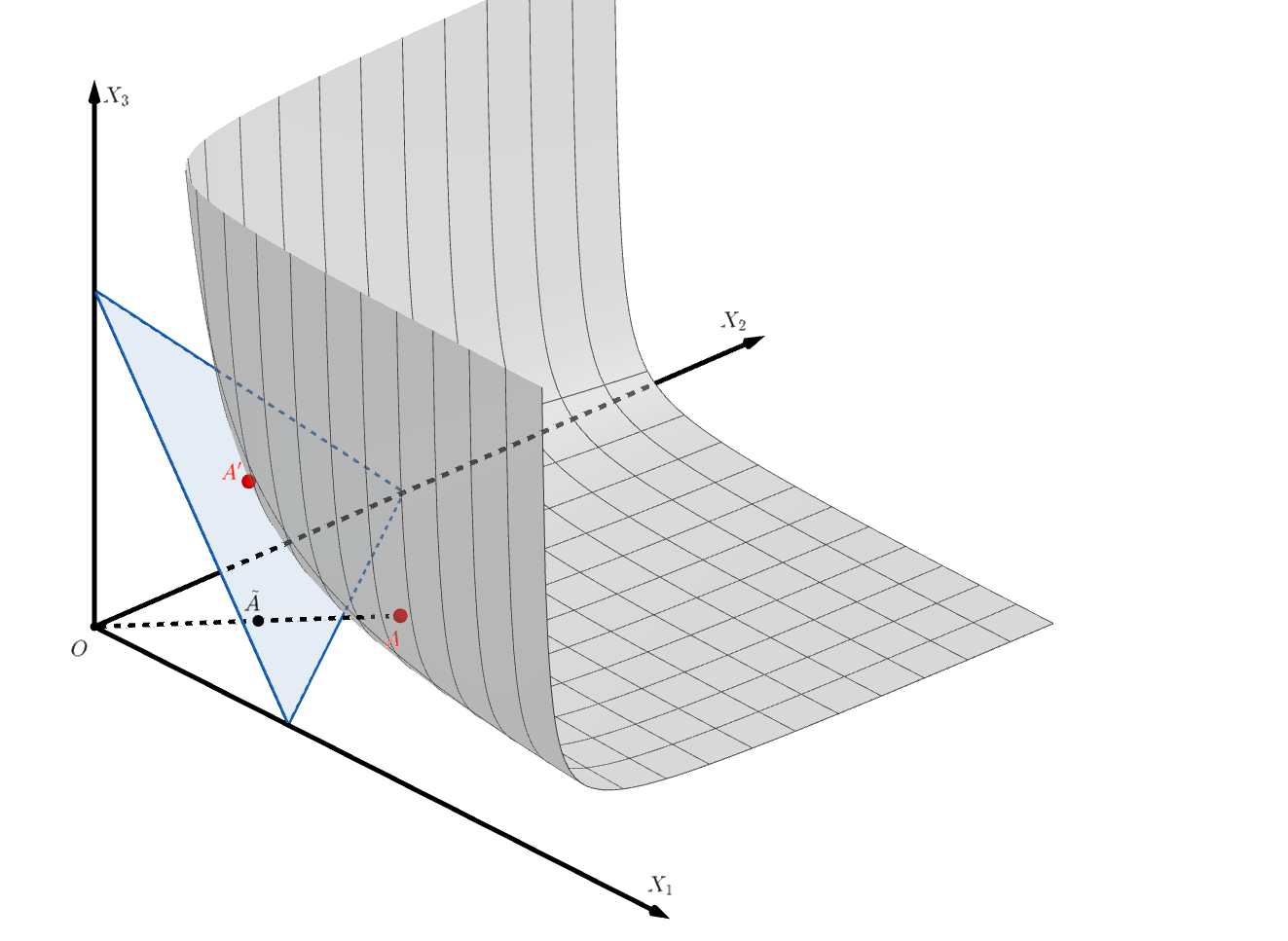
The polar to a point , is the same as the polar to the conic polyhedron and is equal to the conic polyherdon . This polyhedron is obtained by cutting off the corner of the positive orthant by the hyperplane orthogonal to the vector and passing through the point (inverse to the point ). Sometimes we consider this hyperplane is a polar to .
The polar to a conic polyhedron with vertices (in which case ) is the conic polyhedron defined by the system of inequalities .
We see that the duality theory is very similar to what we have in the classical case, with two exceptions. First, the map can be discontinuous [27]. The second one is the self-duality issue addressed in the next section.
2.2. Self-duality
An antinorm on is self-dual if ; a conic body is autopolar if . The self-duality of an antinorm is equivalent to the autopolarity of its unit ball . This means that for an arbitrary point , its polar is a hyperplane of support for , and vice versa (Fig. 1).
Let us remember that in the convex analysis the self-duality is very rare. To avoid a confusion we denote the (classical) polar of a set by . Thus, . The following fact is well-known, we include its proof for convenience of the reader.
Fact. The Euclidean unit ball is a unique subset of such that .
Indeed, if a set coincides with , then . Otherwise, contains a point such that and hence, . On the other hand, the inclusion implies and so, , because and are both autopolar. Hence, .
Thus, apart from the unit Euclidean ball, there are no autopolar sets in . One, therefore, could expect that there are no autopolar conic bodes in either. However, the situation is quite opposite: there are a lot of autopolar conic bodies, including polyhedra. This phenomenon was first observed for in [27]. For general , the orthogonal extensions (preimages of projections) of a planar autopolar body is also autopolar. Are there other examples? The following family of smooth autopolar conic bodies (with smooth strictly convex boundary) was found in [27]. We describe it by the corresponding antinorms:
Example 2
For an arbitrary collection of non-negative numbers such that , the function
| (1) |
(for we set ) is a continuous self-dual antinorm. For example, if , then we obtain a self-dual antinorm in . The corresponding autopolar ball is bounded by the hyperbola.
The function (1) can be rewritten in a simpler form as , where is a constant depending on . There was a mistake in computing this constant in [27], now we correct it. In Proposition 3 we show that the self-duality of (1) follows from the general result of Theorem 1 along with infinitely many other smooth self-dual antinorms.
This was the only known example of nontrivial smooth self-affine antinorm. Theorem 1 from the next section provides a rich variety of other examples.
The problem of existence of nontrivial autopolar conic polyhedra in dimensions was left in [27] and was positively resolved in [16]. For every and , there exists an autopolar conic polyhedron of vertices in . We consider one example for .
Example 3
In the positive orthant we take an arbitrary point on the axis such that (Fig. 2).
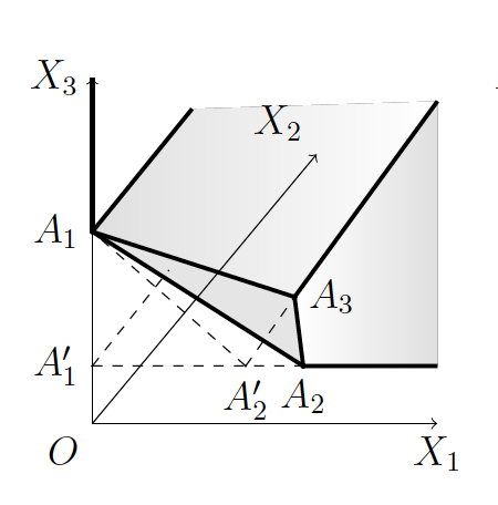
Denote by the polar (hyperplane) to . It is parallel to and passes through the point such that . Denote by the ray of intersection of and the angle . Take an arbitrary point and denote by its polar (hyperplane). Let it intersect at a point . Denote by and the rays of intersection of with and with respectively. Note that the point is the end of . Finally, take a point on such that the three angles and are all right. Such a point exists and unique since the ray is a perpendicular to the plane of the triangle erected at its ortocenter. Denote by the hyperplane of the triangle . Then the conic polyhedron is autopolar. Indeed, it is bounded by three hyperplanes (not counting the coordinate planes) and each plane is a polar to . See [16] for the details.
The polyhedron has three vertices , three facades , and three facades on the coordinate subspaces.
No autopolar polyhedra different from those presented in [16] were unknown. Theorem 1 gives an infinite variety of autopolar bodies both smooth and polyhedral. Before formulating it we observe several general properties of autopolar objects.
Proposition 1
If antinorms and are self-dual and , then .
Proof. The definition of dual antinorm implies that if , then and therefore .
Proposition 2
The distance from every autopolar conic body to the origin is equal to one.
Proof. Let be a self-dual antinorm generated by an autopolar body . Denote by the closest to the origin point of and by the vector . The analogue to Young’s inequality (see above) yields . On the other hand, and hence, , so . Thus, . The hyperplane passing through orthogonal to is a plane of support for . Therefore, its polar , which is the point lies on the unit sphere of the antinorm . Hence, the length of is at least one, therefore and thus, .
Example 4
Applying Proposition 2 to a unit ball of a self-dual antinorm, we see that , whenever . Therefore and this inequality is strict unless is not collinear to . Thus, we obtain
Corollary 1
Every self-dual antinorm does not exceed the Euclidean norm and there is a unique point where they both equal to one.
3. The main results
We begin with Theorem 1 that asserts that every self-dual antinorm can be extended (lifted), from a suitable hyperplane to the whole cone . This lifting is not unique and every dimensional self-dual antinurm can produce infinitely many -demensional ones. This gives a large variety of autopolar conic bodies, both smooth and polyhedral, built inductively. Then we prove Theorem 2 that establishes the structure of those antinorms. For the case , this method gives all autopolar sets (Theorem 3) while for there is an autopolar polyhedron not obtained this way (Example 9).
We call a hyperplane admissible if it has the form , where are two different indices from and is arbitrary. Thus, an admissible hyperplane contains coordinate axes and intersect by an dimensional orthant , which will be denoted as .
3.1. The lifting theorems
Consider an arbitrary admissible hyperplane that splits the orthant into parts . We denote .
Let be an antinorm on , be its unit ball, be its orthogonal extension to defined as , where is the orthogonal projection of to . Thus, is defined on while is defined on . The unit ball of is an intersection of with a right cylinder based on .
Theorem 1
Let an admissible hyperplane split into closed parts and let be a self-dual antinorm on . Let be an arbitrary antinorm which coincides with on and does not exceed on . Then the function defined on by the formula
| (2) |
is a self-dual antinorm on .
Thus, a self-dual antinorm on produces infinitely many such antinorms on . For this, is placed on an arbitrary admissible hyperplane and then an arbitrary antinorm not exceeding the orthogonal extension of can be taken on the part . Then we get a self-dual antinorm by formula (2). The structure of this antinorm is clarified by Theorem 2 below.
Let an admissible hyperplane cut the positive orthant into two closed parts and . Suppose functions are defined on respectively and coincide on ; then their concatenation is defined on as follows:
| (3) |
Thus, and are obtained from each other by the same formula (4). Theorem 1 asserts that the concatenation is a self-dual antinorm on .
Remark 2
The proofs of Theorems 1 and 2 are given in Section 5. We shall see that the admissibility of the plane is used only once: the projection of an arbitrary point to lies in . We are not aware whether it is possible to generalize Theorem 1, maybe in somewhat different form, to an arbitrary hyperplane intersecting the interior of ? Example from Section 6 (Fig. 8) shows that the answer can be affirmative.
3.2. Geometrical formulations
Reformulation of Theorems 1 and 2 in terms of conic bodies is straightforward. For an admissible hyperplane that splits to the parts , (for the sake of simplicity, we assume that they both possess a nonempty interior), denote .
Corollary 2
Let be an admissible hyperplane, be a -dimensional autopolar conic body in . Then for an arbitrary conic body whose intersection with and projection to coincide with , the set , where
| (5) |
is an autopolar conic body in .
Below we use the notation from Corollary 2: the conic body is obtained from by formula (5) and . Let us recall that an orthogonal extension of a set is the preimage of of the orthogonal projection .
Corollary 3
If is autopolar in and the orthogonal extension of every -dimensional plane of support of is a -dimensional plane of support for , then is an autopolar conic body.
If all those planes of support are tangents to and is smooth and strictly convex, then so is . This way one can produce smooth and strictly convex autopolar surfaces. Now turn to conic polyhedra.
Corollary 4
If is an arbitrary conic polyhedron, its facade is autopolar in and all dihedral angles adjacent to this facade do not exceed , then is an autopolar polyhedron.
Let be given by a system of linear inequalities , with all . We add arbitrary linear inequalities such that and the hyperplanes do not intersect the relative interior of . Then the conic polyhedron satisfies the assumptions of Corollary 4. Conversely, every conic polyhedron from Corollary 4 is obtained this way. Each of them produces an autopolar polyhedron in .
3.3. Self-duality in low dimensions
Theorem 1 provides a method of inductive construction of autopolar sets starting with the dimension one.
. This is a trivial case: every antinorm on is a linear function (we do not use the bold letters since we deal with scalars). Then and hence, the only self-dual antinorm is .
. Theorem 1 produces infinitely many self-dual antinorms in . Moreover, it actually gives their complete classification. In this case is a line with , and, respectively, is a ray .
Theorem 1 suggests the following
Algorithm 1 of constructing self-dual antinorms in . We take an arbitrary suitable unit vector and set . This is a self-dual antinorm on . Its orthogonal extension to is . Then choose an arbitrary antinorm on (the angle between and axis) such that and . Geometrically this means that the unit ball is separated from the origin by the perpendicular to erected at the point . Equivalently, the tangent to at the point makes an angle of at most with the ray . Then is defined in by formula (4) and is a self-dual antinorm on .
Theorem 3
Every self-dual antinorm on is obtained by Algorithm 1.
Proof. Let be an arbitrary self-dual antinorm on . Denote by the closest to the origin point of the conic sphere , is the vector . The line passing through and orthogonal to separates from , hence the values of on do not exceed one. By Proposition 2, , hence, for all , . Therefore, by homogeneity, for all . The ray splits into two angles and and the function satisfies all the assumptions of Theorem 1. Hence, the function , where is self-dual. On the other hand, for every , we have
Thus, . Since those functions are both self-dual, we get (Proposition 1).
Corollary 5
Every autopolar conic polygon in has the form , where is an arbitrary ray splitting to two angles, is an arbitrary conic polygon in whose angle at the vertex is at most and is a polar transform of obtained by (5).
4. Examples and special cases
We consider several examples of applications of Theorems 1 and 2 for constructing autopolar sets in general dimensions .
Example 5
(The case of right cylinder). In Theorem 1 one can always take , this is the maximal possible . In this case is a right cylinder with the base . Let separates the axes and and contains the first of them. The function and the set is found by Theorem 2. Its unit ball is an oblique cylinder with base and with the element parallel to the axis. The conic body composed of those two cylinders is autopolar.
Example 6
(The orthogonal extension). In the limit case the hyperplane coincides with one of the coordinate planes, say, the plane . In this case must be equal to . Indeed, if for some , then , where is the th basis vector and is the projection of to . The concavity of the function implies that it becomes negative for large , which is impossible.
Thus, if coincides with a coordinate plane, then and the only feasible conic body is an orthogonal extension of . Hence, the autopolar set produced by Theorem 1 is an orthogonal extension of .
Example 7
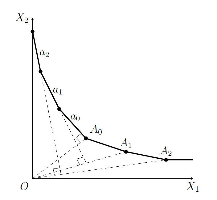
(Autopolar polygons) In view of Theorem 3, every autopolar conic polygon is constructed as follows. We take a point such that and choose an arbitrary conic polygon inside the angle such that the angle of at the vertex is at most . The polygon has two infinite sides: one starting at the vertex parallel to (denote it by ), the other starting at parallel to . This is . Denote by the line which is the polar to . The lines (in this order) form the polygon in the angle . The polygon is autopolar (Fig. 3).
Proposition 3
Proof. We assume that all are nonzero, otherwise we reduce the dimension. Let us show that is obtained by Theorem 1 with the hyperplane and . Introduce the coordinate system in as follows: all the axes are the same as in and the axis . We have
Denote and consider the function on . By the inductive assumption, is self-dual. Then the gradient
belongs to , whenever . Indeed, if , then . Thus, the tangent plane to at every point , is orthogonal to . In view of Corollary 3, we have .
For , the antinorm (1) becomes , which is self-dual. Then every -dimensional antinorm of type (1) can be obtained from this one by steps of Proposition 3 with preserving the self-duality by Theorem 1.
Example 8
The three-dimensional autopolar conic polyhedron presented in Example 3 can be obtained by the lifting form Theorem 1. In this case the hyperplane passes through the axes and through the point , see Fig. 4.
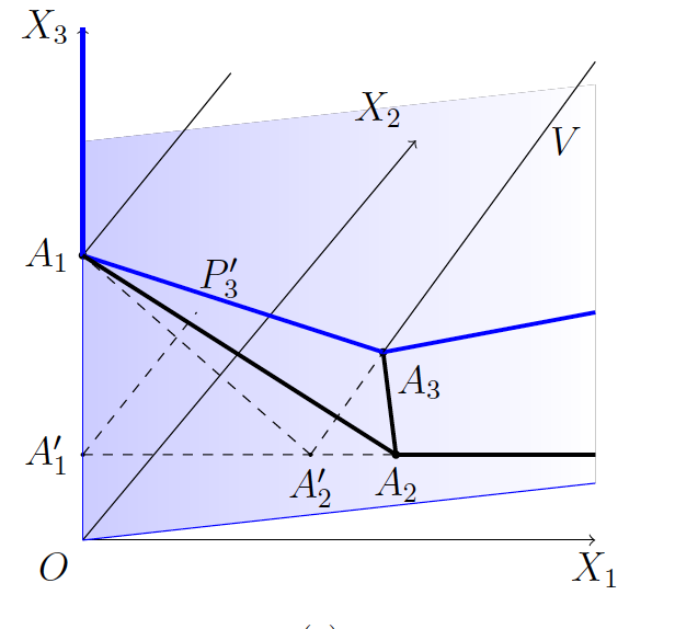
The intersection is a conic polygon bounded by the segment , by the ray , and by the ray going from along the line of intersection of with . The polyhedron is autopolar. Indeed, the polar to is the plane , hence, is obtained by Algorithm 1 with the partition of by the line . Then we pass from to by Corollary 4. The assumptions of the corollary are satisfied. Indeed, is orthogonal to both and and hence, the dihedral angles adjacent to the edges and are right.
5. Proofs of the main theorems
Proof of Theorem 2. For every pair of points , we have and . Therefore,
Take the infimum of the both parts over . In the left hand side we obtain , the right hand side becomes
Thus, for every , we have . On the other hand, an infimum over the set does not exceed an infimum over , hence . Thus, and therefore, .
Now take arbitrary . For every , we have
because and since the vectors and have opposite directions. Thus, . Consequently,
Taking an infimum of both parts over , we conclude that , which proves the inequality on . The proof of 1) is completed.
Take arbitrary and show that for every , there exists for which . This will imply that the infimum of the value over (which is ) is achieved on , i.e., is equal to . This proves the equality for . To establish the existence of a desirable it suffices to take , which means . This follows from two inequalities: a) due to item 1); b) because and hence, the vectors and form a non-obtuse angle, so .
Due to item 1), the function on possess the same properties as on . On the other hand, . Hence, for arbitrary , we argue as above and show that . Invoking now the equality , we conclude the proof of item 2).
Proof of Theorem 1. In the proof of Theorem 2 we showed that . By assertion 2) of Theorem 2, the function is defined by in the same way as is defined by . Interchanging those functions we get . Therefore, . From the definition of the dual function it immediately follows that is an antinorm, hence, so is .
6. A counterexample and open problems
We are giving an example of a three-dimensional conic polyhedron which cannot be obtained by the lifting procedure from Theorem 1. This will leave open the problem of complete classification of autopolar sets (Problem 1 below). We begin with auxiliary results.
For every conic body , the minimal distance to the origin is attained at a unique point . This is a simple consequence of the convexity. If is autopolar, then due to Proposition 2 (Section 2). It turns out that if is obtained by the lifting from an admissible hyperplane , then passes through .
Proposition 4
Assume that an autopolar conic body is obtained by the lifting of a -dimensional conic body from an admissible hyperplane (Theorem 1). Then and have the same point closest to the origin and this point belongs to .
Proof. Let and be the closest to the origin points of the conic bodies and respectively. Since those bodies are both autopolar, it follows that . On the other hand, and belong to and the uniqueness of the closest point yields that .
Thus, if an autopolar body is obtained by Theorem 1, then the splitting hyperplane contains the closest to the origin point . This reduces the search of this hyperplane for a given autopolar set to admissible hyperplanes passing through .
The second property that directly follows from Theorem 2 is the following analogue of Corollary 4. It gives a necessary condition for a conic polyhedron for being obtained by the lifting.
Proposition 5
If a conic polyhedron is obtained by Theorem 1, then the admissible hyperplane intersects by an autopolar -dimensional polyhedron and divides into two polyhedra with a common facade . This common facade makes only non-obtuse dihedral angles with all adjacent facets of and . In particular, every facade of divided by is orthogonal to .
Now we are ready to present the promised counterexample. We use the construction from [16]. To simplify the notation, we sometimes replace the polar by its boundary. For example, the polar of a point is the set . Similarly, we call a polar to a segment the set .
Example 9
The following series of autopolar conic polytopes was presented in [16]. For every , the polytope is constructed in as follows. We take an arbitrary point on the axis such that Then take an arbitrary point on the intersection of the polar to with the hyperplane , see Fig. 5.
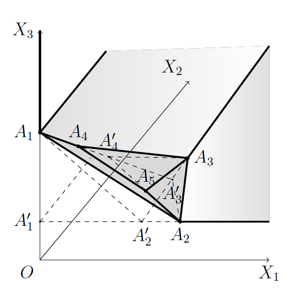
Then the construction is by induction. Suppose the points are constructed, ; then is a point on the polar to the segment such that . Finally, on the last iteration, is chosen on the polar to the segment so that . Then is an autopolar conic polyhedra, for which is the point closest to the origin. The proof is in [16, theorem 2]. Moreover, the construction is well-defined for every choice of points on the corresponding polars under the conditions on the lengths of , see [16]. Therefore, we actually construct a family of autopolar polyhedra and take one of its representatives . Figure 5 presents the polyhedron , Fig. 6 below shows the same polyhedron without auxiliary lines.
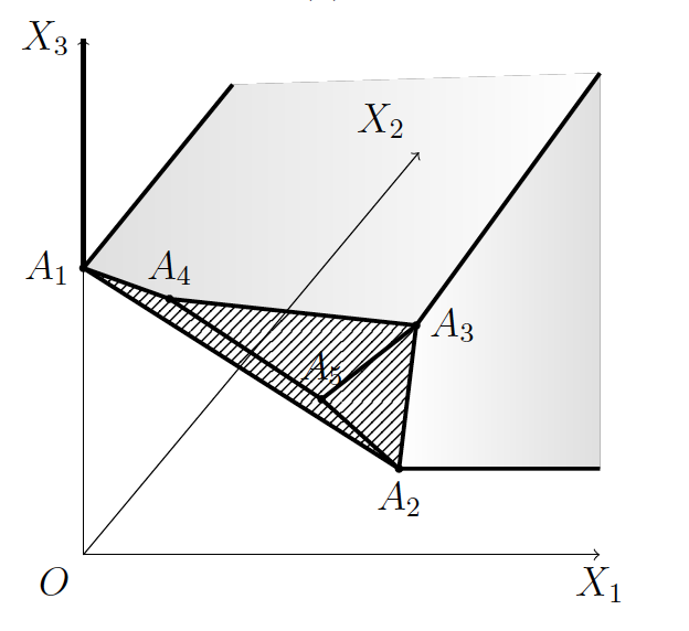
The polyhedron constructed in Example 3 (Fig. 2), also belongs to this series, and actually . As we saw it can be obtained by Theorem 1. The same is true for . It turns out, however, that is not obtained by that theorem, which gives a desired counterexample.
Theorem 4
The conic polyhedron cannot be constructed by the lifting defined in Theorem 1.
Proof. If is constructed by the lifting from an admissible hyperplane , then passes through the closest to the origin point of (Proposition 4). This closest point is [16]. Moreover, due to Proposition 5, is orthogonal to all transversal facades of . If passes through the axis, then it is transversal (and hence, orthogonal) to the facades and , see Fig. 7.
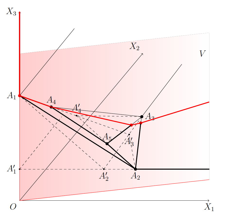
Therefore, is orthogonal to its common edge and hence, is parallel to the coordinate plane . In this case the point lies on the plane , which is the polar to . The latter contradicts to the construction of . The cases when passes to the other coordinate axes are considered in the same way.
Thus, not all -dimensional autopolar conic polyhedra are obtained by the lifting from -dimensional ones. A natural question arises how to classify all possible autopolar sets ?
Problem 1. What is the complete classification of autopolar conic bodies/polyhedra in ?
A complete classification can be either a description of all autopolar conic polyhedra or an algorithm that can construct all of them. Theorem 3 solves this problem for , for higher dimensions it remains open.
A weakened version of Problem 1 is to generalize Theorem 1 to cover all autopolar conic bodies. For example, does there exist a lifting procedure from a non-admissible hyperplane , i.e., non containing coordinate axes? This can be formulated as follows:
Problem 2. Is it true that every autopolar conic polyhedron is split by a hyperplane (possibly non-admissible) orthogonal to all transversal facades of and making non-obtuse angles with all facades intersecting it?
For the polyhedron such a hyperplane exists: this is the plane , see Fig. 8.
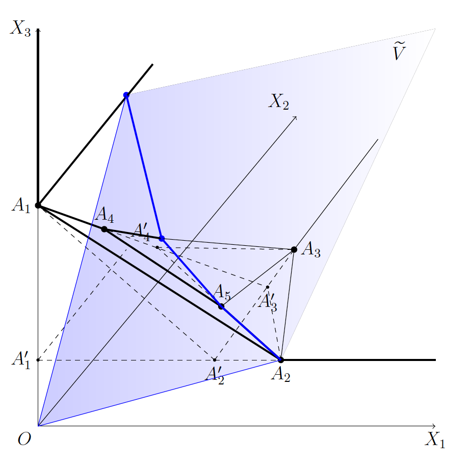
In the proof of Theorem 1 we essentially used the fact that the orthogonal projection of an arbitrary point to is contained in . This is true only for admissible hyperplanes .
References
- [1] F. Blanchini and C. Savorgnanb, Stabilizability of switched linear systems does not imply the existence of convex Lyapunov functions, Automatica, 44 (2008), 1166–1170.
- [2] J.-C. Bourin, F. Hiai, Norm and anti-norm inequalities for positive semi-definite matrices, Internat. J. Math. 22 (2011), 1121–1138.
- [3] J.-C. Bourin, F. Hiai, Jensen and Minkowski inequalities for operator means and anti-norms, Linear Algebra Appl. 456 (2014), 22–53
- [4] J.-C. Bourin, F. Hiai, Anti-norms on finite von Neumann algebras, Publ. Res. Inst. Math. Sci. 51 (2015), 207–235.
- [5] M. Della Rossa and R.M. Jungers, Almost sure Stability of Stochastic Switched Systems: Graph lifts-based Approach, 2022 IEEE 61st Conference on Decision and Control (CDC), Cancun, Mexico, 2022, 1021–1026.
- [6] E. Fornasini and M.E. Valcher, Stability and stabilizability criteria for discrete-time positive switched systems IEEE Trans. Automat. Control 57 (2012), 1208–1221.
- [7] H. Hennion, Limit theorems for products of positive random matrices, Ann. Probab., 25 (1997), 1545–1587.
- [8] N. Guglielmi, L. Laglia, and V.Yu. Protasov, Polytope Lyapunov functions for stable and for stabilizable LSS, Found. Comput. Math., 17 (2017), 567–623.
- [9] N. Guglielmi and V.Yu. Protasov, Exact computation of joint spectral characteristics of linear operators, Found. Comput. Math., 13 (2013), 37–97.
- [10] N. Guglielmi and M. Zennaro, Canonical construction of Barabanov polytope norms and antinorms for sets of matrices, SIAM J. Matrix Anal. Appl. 36 (2015), 634–655.
- [11] N. Guglielmi and M. Zennaro, An antinorm theory for sets of matrices: Bounds and approximations to the lower spectral radius, Linear Algebra Appl. 607 (2020), 89–117.
- [12] R.M. Jungers and V.Yu. Protasov, Lower and upper bounds for the largest Lyapunov exponent of matrices, Linear Algebra Appl., 438 (2013), 4448–4468.
- [13] D. Liberzon, Switching in systems and control, Birkhauser, Boston, MA, 2003.
- [14] H. Lin and P.J. Antsaklis, Stability and stabilizability of switched linear systems: a survey of recent results, IEEE Trans. Autom. Control., 54 (2009), 308–322.
- [15] L.V. Lokutsievskiĭ, Convex trigonometry with applications to sub-Finsler geometry, Sb. Math., 210 (2019), 1179–1205.
- [16] M.S. Makarov, Antinorms and aupotolar polyhedra, Siberian Math. J,, 64 (2023), no 5, 1050-–1064.
- [17] H. Martin and K.J. Swanepoel, Antinorms and Radon curves, Aequationes Math. 72 (2006), 110–138.
- [18] J.K. Merikoski, On antinorms of nonnegative matrices, Linear Algebra Appl. 140 (1990), 31–44.
- [19] J.K. Merikoski, On c-norms and c-antinorms on cones, Linear Algebra Appl. 150 (1991), 315–329.
- [20] J.K. Merikoski, G. de Oliveira, On k-major norms and k-minor antinorms, Linear Algebra Appl. 176 (1992), 197–209.
- [21] A.P. Molchanov and E.S. Pyatnitskii, Criteria of asymptotic stability of differential and difference inclusions encountered in control theory, System Contr. Letters, 13 (1989), 59–64.
- [22] M. Moszyńska and W-D. Richter, Reverse triangle inequality, antinorms and semi-antinorms, Studia Sci. Math. Hungar. 49 (2012), 120–138.
- [23] E. Plischke and F. Wirth, Duality results for the joint spectral radius and transient behaviour, Linear Algebra Appl., 428 (2008), 2368–2384.
- [24] V.Yu. Protasov, Invariant functionals of random matrices, Funct. Anal. Appl. 44 (2010), 230–-233.
- [25] V.Yu. Protasov, Invariant functionals for the Lyapunov exponents of random matrices, Sb. Math., 202 (2011), 101–126.
- [26] V.Yu. Protasov, Asymptotics of products of nonnegative random matrices, Funct. Anal. Appl., 47 (2013), no 2, 138–147.
-
[27]
V.Yu. Protasov,
Antinorms on cones: duality and applications,
Linear and Mult. Alg., 70 (2022), no 22, 7387–7413. - [28] W.-D. Richter, Convex and radially concave contoured distributions, J. Probab. Stat., 2015, Art. ID 165468, 12 pp.
- [29] E. De Santis, M.D. Di Benedetto, G. Pola, Stabilizability of linear switching systems, Nonlinear Anal. Hybrid Syst., 2 (2008), no 3, 750–764.