One-step data-driven generative model via Schrödinger Bridge
Abstract
Generating samples from a probability distribution is a fundamental task in machine learning and statistics. This article proposes a novel scheme for sampling from a distribution for which the probability density for is unknown, but finite independent samples are given. We focus on constructing a Schrödinger Bridge (SB) diffusion process on finite horizon which induces a probability evolution starting from a fixed point at and ending with the desired target distribution at . The diffusion process is characterized by a stochastic differential equation whose drift function can be solely estimated from data samples through a simple one-step procedure. Compared to the classical iterative schemes developed for the SB problem, the methodology of this article is quite simple, efficient, and computationally inexpensive as it does not require the training of neural network and thus circumvents many of the challenges in building the network architecture. The performance of our new generative model is evaluated through a series of numerical experiments on multi-modal low-dimensional simulated data and high-dimensional benchmark image data. Experimental results indicate that the synthetic samples generated from our SB Bridge based algorithm are comparable with the samples generated from the state-of-the-art methods in the field. Our formulation opens up new opportunities for developing efficient diffusion models that can be directly applied to large scale real-world data.
Keywords: Diffusion process; Generative model; Neural network; Sampling; Stochastic differential equation.
1 Introduction
Generating samples efficiently from complex probability distributions plays a key role in a variety of prediction and inference tasks in machine learning and statistics. We have two types of settings. In the first setting, the probability distribution for is explicitly given. This is often the case in Bayesian statistics. In the second setting, the explicit form of is not specified, but we have access to a collection of i.i.d. random samples. This is the case in generative modeling which has been extensively studied over the last years and has found wide-ranging applications across diverse domains such as computer vision (Huang et al., 2021b, ; Sohl-Dickstein et al.,, 2015; Endo and Kanamori,, 2020), image analysis (Wang and Ponce,, 2021; Pu et al.,, 2015), natural language processing (Shah,, 2021; Fu,, 2019; Miao,, 2017), drug discovery (Chen et al., 2023b, ; Zeng et al.,, 2022), and recommendation systems (Liu et al.,, 2021). Most of the existing generative models seek to understand the underlying data generating mechanisms through learning a nonlinear function that can transform a simple reference distribution to the target distribution. Here we focus on a powerful class of generative models, called the diffusion models which have achieved enormous success in synthesizing high-fidelity data. Instead of assume a specific form of the data distribution, the diffusion models implement a stochastic process and use its endpoint to represent the target distribution. Two promising approaches in diffusion models are score based diffusion models (Sohl-Dickstein et al.,, 2015; Ho et al.,, 2020; Song et al., 2021a, ; Song et al., 2021b, ) and Schrödinger Bridge based diffusion models (Bernton et al.,, 2019; Chen et al., 2023a, ; Bortoli et al.,, 2023; Shi et al.,, 2023; Chen et al., 2023c, ; Liu et al.,, 2023; Stromme,, 2023).
The score based generative models (SGM) consist of two processes: the noise-injecting process also called the forward process and the denoising process also called the backward process. The forward process is implemented by incrementally adding noise to the original data until they are indistinguishable from samples drawn from a easily sampled prior distribution, e.g., the Gaussian distribution. The backward process is implemented by recovering the original data distributions from the prior. Both processes can by modeled as stochastic processes in terms of a stochastic differential equation (SDE). The drift function for the forward SDE is defined such that the desired prior becomes the marginal distribution of the process at the end time. Similarly, the drift function for the backward SDE is defined such that it can be used to generate data samples from the prior. The basis of SGM lies in the notion of the score function (i.e. the gradient of the log-density function of a given distribution) which can be learned (often parametrized by neural network) through regression at each time step.
Despite its empirical success, the diffusion process of SGM needs to run sufficiently large time steps so that the end distribution is approximately Gaussian. To overcome this limitation, an alternative approach based on the so-called Schrödinger Bridges (SB) has been proposed which allows one to obtain exact samples from a sufficiently well-behaved target density in finite time. This approach, going back to a problem posed by Schrödinger in the 1930s in the context of physics (Schrödinger,, 1932; Chetrite et al.,, 2021), tries to construct a stochastic process that has two given distributions as marginals at the initial and end times, while subject to a reference process. SB can also be formulated as an entropically regularized optimal transport problems which seeks optimal policies to transform the probability density between given arbitrary initial and end distributions in a finite horizon. Despite its attractiveness, the numerical solution of SB problems are usually based on the so-called Iterative Proportional Fitting (IPF) algorithm (also known as the Sinkhorn algorithm) which is computationally more demanding in contrast to the SGM methods (Chen et al.,, 2021). IPF solves the bridge problem by creating a convergent sequence of forward and backward processes, known as half-bridges, in which only one of the two distributions at the boundaries of the time interval is kept fixed. The drift function for the corresponding SDE of a half-bridge is learned from samples created by the half-bridge of the previous iteration using a regression approach via training a deep neural network. This approach is deemed as computationally too demanding because the drift at a given iteration is represented as a sum of scores obtained in the previous steps. Moreover, it requires the storage of an increasing number of neural networks, two per iteration. Consequently, practical usages of SB for learning high-dimensional data distributions is limited for these reasons.
In this work, we propose an efficient method to generate samples from a distribution for which the probability density is unknown, but a finite set of sample points are provided. Our approach is based on Euler-Maruyama discretization of a tractable class of SB diffusion processes, defined on the unit time interval , that transport the degenerate Dirac delta distribution at time zero to the target distribution at time one. We show that, given such boundary pairs, the solutions of the SB system admit analytic forms which solely rely on the given data samples and thereby yield a simulation-free framework that avoids unfavorable complexity occurring in many simulation-base algorithms. Our approach differs from prior SB based work in that it is a one-step solution which does not need to run iteration. Moreover, our method scales well to high-dimensions as it does not require training neural network and thus substantially reduces the computation burden. We demonstrate the practical use of our algorithm on simulated and real-world data by quantitatively and qualitatively comparing its performance to the state-of-the-art methods in the field.
A fundamental difference between our SB based approach and many existing related works is that we start the process from a Dirac delta distribution instead of a Gaussian distribution. For Gaussian and target boundary pair, usually the SB problem has no closed form solution and one has to rely on iterative schemes. In addition to IPF, various other type of iterative algorithms have been proposed in the literature. Examples include Bernton et al., (2019); Vargas et al., (2021); Pavon et al., (2021); Chen et al., 2023a ; Winkler et al., (2023); Bortoli et al., (2023); Winkler et al., (2023); Chen et al., (2021); Shi et al., (2023); Chen et al., 2023c ; Liu et al., (2023); Lee et al., (2024) and many others. Recently, the Schrödinger-Föllmer process (SFP) has been used for developing sampling scheme which considers the same boundary pair and transports the delta distribution at time zero to the target distribution at time one. For example, the SFP based algorithms are proposed in Zhang and Chen, (2022); Huang et al., 2021a for drawing samples from the target density which is known up to a normalizing constant. This approach is also applied to the problem of Bayesian inference in Vargas et al., (2022). Our method is different from these SF based approaches in that we are considering sampling scheme from distributions which are known only through a finite set of sample points. Wang et al., (2021) present a a two-stage deep generative model based on SF, in which the first stage learns a smoothed version of the target distribution, and the second stage derives the actual target at the sample level. Our method can be considered as a one-step simplification of this approach and therefore is more computationally simple. Most closely related to the current paper are results by Hamdouche et al., (2023) that derives a generative model for time series based on SFP approach in which the drift function is directly estimated from the data samples. The major difference is that Hamdouche et al., (2023) focuses on the time series problem, while we focus on the problem of drawing samples from arbitrary probability distributions. In contrast to the above SFP based algorithms that only consider standard Brownian motion as reference process, our approach is more flexible and allows the reference process to be any Ito’s process. It is shown in the numerical studies in Section 3 that the performance of our algorithm in some situations can be significantly improved by appropriately choosing the reference process.
The paper is organized as follows. In Section 2, we provide an introduction to Schrödinger bridge diffusion process and present a class of tractable Schrödinger system of which the solution can be explicitly derived. Then we propose a one-step data-driven generative model and outline its implementation algorithm. Section 3 is devoted to numerical studies. We test the performance of our algorithm on both simulated low-dimensional data and real-world high-dimensional image data. Concluding remarks are given in Section 4. Proof for the theorem is provided in Appendix A.
2 Data-driven Schrödinger Bridge sampler
In this section we first provide some background on the Schrödinger Bridge process. Then we introduce a class of tractable Schrödinger Bridge processes. Finally we propose a novel generative model based on this tractable class by appropriately choosing the reference SDEs.
2.1 Background on Schrödinger Bridge
We are interested in generating synthetic data from an unknown distribution for which we have a data set of i.i.d. samples , . Our algorithms are implemented through constructing a stochastic diffusion process indexed by a continuous time variable such that , the Dirac delta distribution centered at , and , the target distribution. Denote by the space consisting of all -valued continuous functions on the time interval and the measure over induced by the following SDE
| (2.1) |
where is the standard -dimensional Brownian motion, is a vector-valued function called the drift coefficient of , and is a scalar function known as the diffusion coefficient of . When and , is just the standard -dimensional Brownian motion. The SDE (2.1) has a unique strong solution as long as the drift coefficient function is globally Lipschitz in both state and time (Oksendal,, 1992).
Denote by the marginal probability law at time for the probability measure on . We write for the set of all path measures with given marginal distribution at the initial time and at the final time. Then the solution of the Schrödinger Bridge (SB) problem with respect to the reference measure can be formulated by the following optimization problem
| (2.2) |
where denotes the relative entropy between two probability measures on and which is defined as
| (2.5) |
where denotes that is absolutely continuous w.r.t. and represents the Radon-Nikodym derivative of w.r.t.
2.2 A tractable class of Schrödinger Bridge
It is known (Pavon,, 1989; Dai Pra,, 1991; Leonard,, 2014) that if the reference process is induced by (2.1), then is induced by a SDE with a modified drift:
| (2.6) |
When and , i.e. is a Wiener measure, the SB problem (2.2) with initial margin is also called the Schrödinger-Föllmer process (SFP). The properties of SFP have been explored in Dai Pra, (1991); Leonard, (2014); Tzen and Raginsky, (2019); Huang et al., 2021a ; Vargas et al., (2022); Zhang and Chen, (2022) via closed form formulation of the drift in terms of expectations over Gaussian random variables known as the heat semigroup. These work also explores how the formulation of the SFP can be used in practice to construct exact sampling schemes for target distributions. Particularly, the work by Huang et al., 2021a investigates how to estimate the SFP drift in practice via the heat semigroup formulation using a Monte Carlo approximation. Vargas et al., (2022) applies the SFP drift estimation to the problem of high-dimensional Bayesian inference. Zhang and Chen, (2022) proposes a similar algorithm to estimate the normalizing constant of un-normalized densities.
Most of the prior studies on how to use SFP to generate samples are analytical, taking as input the pre-specified probability densities. Our approach in this work, instead, inspired by the original idea of Schrödinger, applies to situations where only samples are available. Moreover, the reference measure in our proposal is not restricted to the Wiener process, i.e. and in (2.1) can be any function as long as they yield a closed form solution for .
Denote the gradient of a smooth function by and the partial derivative with respect to of for by . To facilitate the reformulation of the problem so that it involves the target distribution only through its available samples, we state in the following theorem the solution of the SB problem (2.2) whose reference measure is induced by the SDE (2.1) with and/or .
Theorem 1.
Assume that and the components of are bounded continuous and satisfy Holder conditions with respect to , i.e. there are real constants such that for all and . Further assume that is absolutely continuous. Then the stochastic process (2.6) induces a probability measures which solves the Schrodinger Bridge problem (2.2) if the drift term is given by
| (2.7) |
where
| (2.8) |
with denotes the transition density of at time given at time for stochastic process governed by the reference SDE (2.1).
Theorem 1 shows that we can start from any point and update the values of according to the SDE (2.6) in continuous time, then the value has the desired distributional property, that is, . Note that the drift function (2.7) is also the solution of the following stochastic control problem
| (2.9) | |||||
| (2.12) |
A nice property of the stochastic control framework (2.9) is that it enables us to design efficient sampling scheme via transporting particles on any fixed single point to the particles drawn from the target distribution on the unit time interval (Zhang and Chen,, 2022).
2.3 Drift estimation
The drift term (2.7) involves the integration over the target distribution which usually has no closed form solutions. We are considering the frequently occurring situation where is only known through a fixed set of samples. In order to evaluate the integration in (2.7) accurately, we need to find a good estimation for the probability density from the given samples. This is quite challenging especially in high-dimensional cases because the underlying distribution often has multi-modes or lies on a low-dimensional manifold, which cause difficulty to learn from simple distribution such as Gaussian or mixture of Gaussian. Many methods have been proposed to form useful estimates of typical of which are the kernel method (Parzen,, 1962), the interpolation method (Wahba,, 1975), and diffusion based method (Masry,, 1983). These traditional methods are mainly designed for low-dimensional cases and fall short in scaling to high-dimensions. Wang et al., (2021) obtained the estimator of probability density via minimizing an empirical logistic regression loss determined by the score function that can be modeled using a deep network. However, this method is very costly and prone to high variance as it requires the training of the neural network.
In this work, we instead take two advantages of formula (2.7) and propose an alternative one-step estimation for the drift coefficient . The first advantage is that it involves expectations under the target distribution , so its integral can be replaced by its empirical counterpart, i.e.
| (2.13) |
which leads to the following direct estimation
| (2.14) |
This one-step solution does not require the training of deep neural network and avoids the complexity of building the network architecture and thus is computationally more inexpensive. The second advantage is that the transition density in (2.8) is for the reference process which can be obtained in closed-forms by appropriately choosing the drift function and diffusion function in (2.1). For example, when is affine in terms of , the transition kernel is always a Gaussian distribution denoted by , where the mean and covariance matrix are often known and can be obtained with standard techniques.
2.4 Reference SDEs
In numerical studies, we consider three choices of reference SDEs proposed in Song et al., 2021b which have been successfully used in many probabilistic generative tasks. All of them can yield closed form solutions for both the transition probability and the drift .
-
•
Variance exploding (VE) SDE:
(2.15) where , is a -dimensional identity matrix and
(2.16) where denotes the -norm. If we choose , it is just the standard -dimensional Brownian motion.
-
•
Variance preserving (VP) SDE:
(2.17) where
-
•
Sub-Variance preserving (sub-VP) SDE:
(2.18) where
The VE SDE yields a process with exploding variance when . In contrast, the VP SDE yields a process with bounded variance. In addition, the VP process has a constant unit variance for all when the initial distribution of has a unit variance. The two successful classes of score-based generative models: score matching with Langevin dynamics (SMLD) and denoising diffusion probabilistic modeling (DDPM) are discretization of VE SDE and VP SDE respectively (Song et al., 2021b, ). In SMLD, one has for which leads to a diffusion coefficient . In DDPM, one has which leads to a diffusion coefficient . The detailed choice of and in our algorithm is discussed in Section 3.1. It is worth mentioning that the noise level is annealed up in both SMLD and DDPM while it is annealed down in our implementation as our SB process corresponds to the reverse-time process of SMLD and DDPM.
Note that even if is known, the closed form expression for the drift term can only be obtained in some special situations. For example, if is Gaussian mixture, Huang et al., 2021a derived the explicit expression of the drift terms for VE SDE with . We derive the corresponding results for VP SDE with general in Section B.
2.5 Euler-Maruyama discretization
Once the drift function is determined, the diffusion process (2.6) can be used to sample from the target distribution by transporting the initial degenerate distribution at to the target at . The fact that the SDE (2.6) is defined on the finite time interval allows us to numerically implement this approach simply through Euler-Maruyama discretization. We first take grid points on with and being the step size for the -th interval. Then the resulting discretization of the diffusion process (2.6) is
| (2.19) |
where are independent and identically distributed random vectors from . If the reference process is induced by VE SDE, the drift term can be estimated as
| (2.20) |
where is defined in (2.16). The drift terms for other reference SDEs can be estimated in a similar way. Based on (2.19), we can start from and iteratively update this initial value to obtain a realization of the random sample which is approximately distributed as the target distribution under suitable conditions. For convenience, we shall refer to the proposed sampling method as the data-driven Schrödinger Bridge sampler (DSBS). The pseudocode for implementing DSBS is presented in Algorithm 1.
Note that, in contrast to Langevin diffusion based sampling approaches which rely on the diffusions that reach the target distribution as their equilibrium state when time goes to infinity, the SB based dynamics are controlled and the target distribution is reached in finite time. An advantage of our DSBS sampling scheme over the traditional MCMC based methods is that ergodicity is not required (Huang et al., 2021a, ). This is also due to the basic property of the SB diffusion (2.6) which transports the initial distribution at to the exact target distribution at . The sampling error of DSBS is entirely due to the approximation of the drift term via (2.20) and the Euler-Maruyama discretization via (2.19). The first type of approximation errors can be well controlled by the large sample theorem according to (2.13). The second type of approximation errors can also be made arbitrarily small under suitable conditions as shown in Huang et al., 2021a .
3 Numerical experiments
In this section, we demonstrate the effectiveness of our algorithm on several simulated and real data sets. We first employ two-dimensional toy examples to show the ability of our algorithm to learn multimodal distributions. Next, we show that our algorithm is able to generate realistic image samples. We use two benchmark datasets including MNIST (LeCun and Cortes,, 2010) and CIFAR-10 (Krizhevsky and Hinton,, 2009).
3.1 Setup
We have compared the numerical results of DSBS using three types of reference SDEs introduced in 2.4 and found that the performance of sub-VP is worse than VE and VP in all the data sets to which we applied. Therefore, we only report the results for VE and VP here which are denoted by VE-DSBS and VP-DSBS respectively. For VE models, the noise scale is chosen to be . The corresponding reference SDE process is just the standard Brownian motion, i.e. , and its perturbation transition kernel can be derived as . Usually VE models normalize image inputs to the range . For VP models, we let with or . This corresponds to the following instantiation of the VP SDE:
| (3.1) |
The perturbation kernel is given by
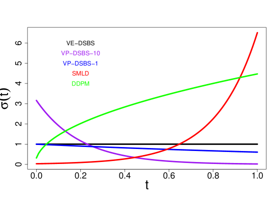
Figure 2 compares the diffusion function used in various diffusion models including VE-DSBS, VP-DSBS with , VP-DSBS with , SMLD, and DDPM. The two score based generative models, SMLD and DDPM, involve sequentially corrupting data with slowly increasing noise, therefore their diffusion functions increase with as shown by the red and green curves in Figure 1. On the other hand, our SB based approaches reverse the step and thus form a sequence of decreasing noise scales. This is why their corresponding diffusion functions decrease with or keep to be a constant as shown by the purple, blue, and black curves in Figure 1.
In our experiment, we use the Euler-Maruyama discretization for the SDE (2.19) with a fixed step size, i.e. .
3.2 Learning low-dimensional distributions
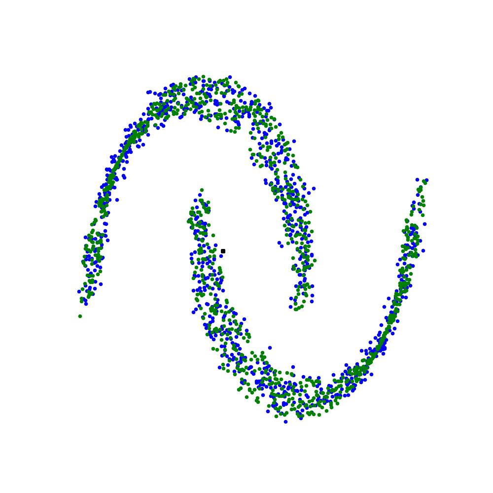
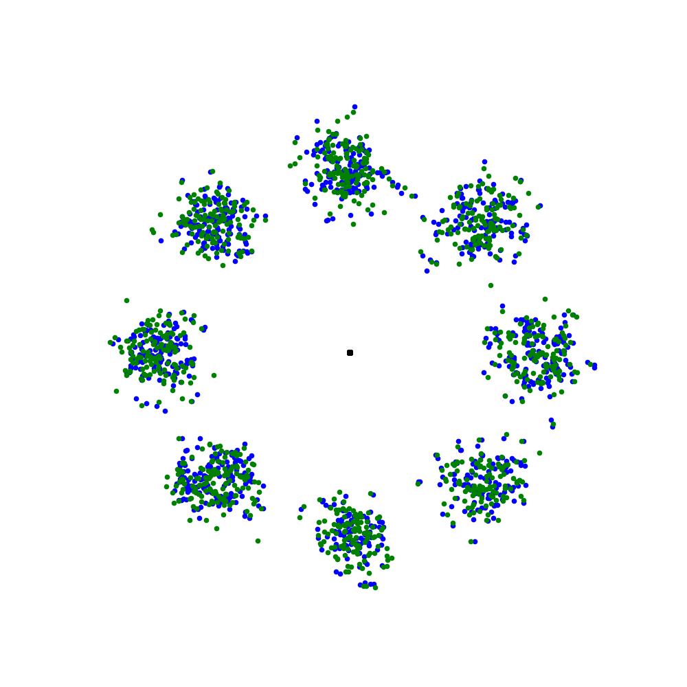
We first evaluate how well various methods can effectively learn multi-modal distributions on low-dimensional data sets. We follow the setup from Shi et al., (2023); Tong et al., 2024b and use two common benchmark examples to illustrate and compare the different approaches. The first example is the Moons data which is sampled from a complicated distribution whose support is split into two disjoint regions of equal mass shaped like half-moon (Pedregosa et al.,, 2011). The second example is 8-Gaussians data which is generated from a mixture of Gaussians with 8 components which are relatively far away from each other. Similar to the methods and models reported in Tong et al., 2024b , we use a training set size of 10000 and a test set size of 10000. We let the starting point and set the number of discretization steps . We run each setting 10 times with mean and standard deviation reported. Figure 2 compares the training samples (green) with the samples generated from our DSBS method (blue). They are very close and all the modes are included in both examples.
We evaluate the empirical 2-Wasserstein distance for 10000 generated samples from our model. The value reported for is
where is sampled via our algorithm, is the test set, and is the set of all couplings of and . We report the 2-Wasserstein distance between the predicted distribution and the target distribution with test samples of size 10000. Table 1 summarizes the comparison of our approaches with the following methods:
-
•
Simulation-Free Schrödinger Bridges via Score and Flow Matching (Tong et al., 2024b, ) with exact optimal transport couplings (M-exact) and with independent couplings (M-I);
-
•
Iterative Schrödinger bridge models: diffusion Schrödinger bridges (DSB) and diffusion Schrödinger bridge matching with algorithms based on iterative proportional fitting (DSBM-IPF) and Iterative Markovian Fitting (DSBM-IMF);
-
•
ODE flow-based models: optimal transport conditional flow matching (OT-CFM), Schrödinger bridges conditional flow matching (SB-CFM), independent conditional flow matching (I-CFM), rectified flow (RF), and flow matching (FM).
The results derived from SDE based stochastic methods and ODE based deterministic methods are put in the top and bottom blocks in Table 1 respectively. They are reported in Tong et al., 2024b . For 8-gaussians data set, VE-DSBS outperforms all methods and VP-DSBS-10 is in the third place. For Moons data set, VE-DSBS is in the fifth place. The performance of VE-DSBS is better than the performance of VP-DSBS-1 and VP-DSBS-10 on both data sets. The results from Table 1 show that DSBS is a competitive generative model for low-dimensional data.
| Algorithm | 8-Gaussians | Moons |
| VE-DSBS | 0.148 (0.026) | |
| VP-DSBS-1 | 0.316 (0.062) | 0.185 (0.020) |
| VP-DSBS-10 | 0.293 (0.077) | 0.329 (0.036) |
| M-exact (Tong et al., 2024b, ) | 0.275 (0.058) | |
| M-I (Tong et al., 2024b, ) | 0.393 (0.054) | 0.185 (0.028) |
| DSBM-IPF (Shi et al.,, 2023) | 0.315 (0.079) | 0.140 (0.006) |
| DSBM-IMF (Shi et al.,, 2023) | 0.338 (0.091) | 0.144 (0.024) |
| DSB (Bortoli et al.,, 2023) | 0.411 (0.084) | 0.190 (0.049) |
| OT-CFM (Tong et al., 2024a, ) | 0.303 (0.053) | 0.130 (0.016) |
| SB-CFM (Tong et al., 2024a, ) | 2.314 (2.112) | 0.434 (0.594) |
| RF (Liu,, 2022) | 0.421 (0.071) | 0.283 (0.045) |
| I-CFM (Tong et al., 2024a, ) | 0.373 (0.103) | 0.178 (0.014) |
| FM (Lipman et al.,, 2023) | 0.343 (0.058) | 0.209 (0.055) |
3.3 Image Generation
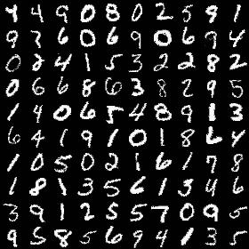
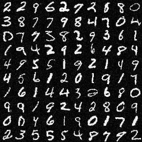
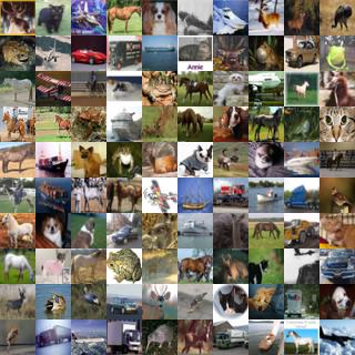
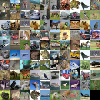
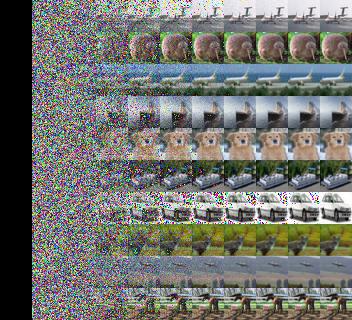
Next, we validate our method on high-dimensional image generation. We consider the well-studied MNIST and CIFAR10 data sets. The MNIST data set consists of gray-valued digital images, each having 2828 pixels and showing one hand-written digit. The generated images for MNIST using the DSBS algorithm based on 10000 training samples are presented in Figure 3, which clearly suggest that our method is able to synthesize high-fidelity images. The CIFAR10 data set consists of 60000 images in 10 classes, with 6000 images per class. The images are colored and of size 3232 pixels. Figure 4 shows the generated samples and their comparison with the true samples on CIFAR10. As the Figure demonstrates, our algorithm successfully generates sharp, high-quality, and diverse samples on high-dimensional image. Figure 5 shows the progressive generation on CIFAR10 in our algorithm. It shows that our approach provides a valid path for the particles to move from a fixed point at to the target distribution at .
Table 2 summarizes the Fréchet Inception Distance score (FID) (Heusel et al.,, 2018) on CIFAR10 of our algorithm as well as other two type of state-of-the-art generative models: Optimal Transport (OT) methods and score based generative models (SGM). The OT type of methods include SB-FBSDE, forward-backward SDE (Chen et al., 2023a, ), DOT, discriminator optimal transport (Tanaka,, 2023), multi-stage SB (Wang et al.,, 2021), and DGflow, deep generative gradient flow (Ansari et al.,, 2021). The SGM type of models include ScoreFlow, score-based generative flow (Song et al., 2021a, ), VDM, variational diffusion models (Kingma et al.,, 2023), and LSGM, latent score-based generative model (Vahdat et al.,, 2021). The FID score is a metric used to assess the quality of images created by a generative model. It compares the distribution of generated images with the distribution of a set of real images. We report the FID over 30k samples w.r.t. the training set. Notably, our method achieves score 3.88 on CIFAR10, which is comparable to the top existing SGM type of methods and outperforms most of the other OT type of methods by a large margin in terms of the sample quality. We omit FID scores on MNIST as the scores on this data set are not widely reported.
| Model Class | Method | FID |
| Optimal Transport | VP-DSBS-10 (ours) | 3.88 |
| SB-FBSDE (Chen et al., 2023a, ) | 3.01 | |
| DOT (Tanaka,, 2023) | 15.78 | |
| Multi-stage SB (Wang et al.,, 2021) | 12.32 | |
| DGflow (Ansari et al.,, 2021) | 9.63 | |
| SGMs | SDE (deep, sub-VP; Song et al., 2021b ) | 2.92 |
| ScoreFlow (Song et al., 2021a, ) | 5.7 | |
| VDM (Kingma et al.,, 2023) | 4.00 | |
| LSGM (Vahdat et al.,, 2021) | 2.10 |
4 Conclusion
In this article, we propose a novel class of simulation-free generative model for sampling from distributions which are known only through a finite set of samples. The procedure is through Euler-Maruyama discretization of a tractable class of Schrödinger bridge diffusion process whose initial distribution is of degenerate type, i.e. the process starts from a fixed point. We obtain the solution of the diffusion process by deriving the explicit formulation for the drift function of its corresponding SDE. The formulation turns out to be quite simple and relies solely on data samples and the transition probability of the reference process. Our approach is more flexible than existing related works in that its reference process is not limited to standard Brownian motion but can be any Ito’s process. We consider three type of reference SDEs: VE, VP, and sub-VP in our numerical studies and all of them have closed form expressions. The usefulness of our method is demonstrated through application to both low-dimensional simulated data and high-dimensional image data. The numerical results show that our method is competitive with the state-of-the-art generative models. The biggest advantage of our method is that it is simple, efficient, and low cost computationally as it is a one-step procedure and does not involve iteration and training the neural network.
Our formulation opens up new algorithmic opportunities for developing efficient nonlinear diffusion models that have a broad scope of applicability. We plan to apply our method to more real-world data. We have considered three prior processes in our implementation and observed that the performance depends on the prior process and the optimal choice of the prior is different for different data sets. Many applications require more general priors whose distributions are not available in closed form if one considers SDEs with nonlinear drift functions. Future work can consider how to extend the present methodology to general situations and find the way on how to choose optimal prior process for given data samples.
Appendix A Proof of Theorem 1
Proof.
Assume that is absolutely continuous with respect to the reference measure , i.e. . The disintegration theorem then gives
| (A.1) |
where (respectively, ) denotes the conditional probability law of given under (respectively, ). The conditional probability measure gives the probability law of the reference process which usually has a closed form solution. Now since , we have , whereas for the reference process . Thus we have the following expression for the right hand side of (A.1)
where equality holds if and only if almost everywhere. This immediately implies that and the above infimum is attained by the probability measure , i.e. by the -mixture of reference processes .
Recall that the path measure describes a solution to the following SDE
We first make the gradient ansatz and assume that the diffusion process is governed by an Ito SDE of the form
| (A.2) |
where denotes the gradient with respect to the space variable. Then we will show that we can choose a suitable function which is twice continuously differentiable in and once differentiable in such that the probability law of the resulting process defined in will be governed by .
Given two Ito processes with the same diffusion, we can use the Girsanov theorem to write down the Radon-Nikodym derivative of with respect to by
| (A.3) |
Let us define the process by . Ito’s lemma then gives
where is the Laplacian. Integrating and rearranging, we obtain
Substituting this into (A.3) and using the definition of gives
Let solves the PDE
| (A.4) |
for all subject to the terminal condition and . Now the PDE (A.4) is nonlinear in due to the presence of the squared norm of the gradient of on the right hand side. From the theory of PDE we can convert it into a linear PDE by making the logarithmic transformation which is also called the Cole-Hopf transformation (Hopf,, 1950). Substituting this into (A.4), we obtain a much nicer linear PDE for :
| (A.5) |
on subject to the terminal condition and . Let us again define the process by and apply Ito’s lemma:
where we have used the fact that solves (A.5). Taking integration we obtain
Taking conditional expectation on both side given , we obtain
| (A.6) |
for any and , where is defined in (2.8). This is also called the Feynman-Kac formula for the solution of (A.5), one of the remarkable connections between the theory of PDE’s and diffusion processes. To verify that the terminal conditions are satisfied, we obtain
Then transform (A.6) for into and substitute into (A.2), we obtain
which leads to (2.7), i.e.
∎
Appendix B Gaussian mixture distributions
Assume that the target distribution is a Gaussian mixture, i.e.,
where is the number of mixture components. For VP SDE, the drift coefficient (2.17) can be written as
where
where
References
- Ansari et al., (2021) Ansari, A. F., Ang, M. L., and Soh, H. (2021). Refining deep generative models via discriminator gradient flow. arXiv:2012.00780.
- Bernton et al., (2019) Bernton, E., Heng, J., Doucet, A., and Jacob, P. E. (2019). Schrödinger bridge samplers. arXiv:1912.13170.
- Bortoli et al., (2023) Bortoli, V. D., Thornton, J., Heng, J., and Doucet, A. (2023). Diffusion schrödinger bridge with applications to score-based generative modeling. arXiv:2106.01357.
- (4) Chen, T., Liu, G.-H., and Theodorou, E. A. (2023a). Likelihood training of schrödinger bridge using forward-backward sdes theory. arXiv:2110.11291.
- Chen et al., (2021) Chen, Y., Georgiou, T. T., and Pavon, M. (2021). Optimal transport in systems and control. Annual Review of Control, Robotics, and Autonomous Systems, 4(Volume 4, 2021):89–113.
- (6) Chen, Y., Wang, Z., Wang, L., Wang, J., Li, P., Cao, D., Zeng, X., Ye, X., and Sakurai, T. (2023b). Deep generative model for drug design from protein target sequence. Journal of Cheminformatics, 15(1):1 – 12.
- (7) Chen, Z., He, G., Zheng, K., Tan, X., and Zhu, J. (2023c). Schrodinger bridges beat diffusion models on text-to-speech synthesis. arXiv:2312.03491.
- Chetrite et al., (2021) Chetrite, R., Muratore-Ginanneschi, P., and Schwieger, K. (2021). E. schrödinger’s 1931 paper “on the reversal of the laws of nature” [“Über die umkehrung der naturgesetze”, sitzungsberichte der preussischen akademie der wissenschaften, physikalisch-mathematische klasse, 8 n9 144–153]. The European Physical Journal H, 46(1).
- Dai Pra, (1991) Dai Pra, P. (1991). A stochastic control approach to reciprocal diffusion processes. Applied Mathematics and Optimization, 23(1):313–329.
- Endo and Kanamori, (2020) Endo, Y. and Kanamori, Y. (2020). Diversifying semantic image synthesis and editing via class‐ and layer‐wise vaes. Computer Graphics Forum, 39(7):519–530.
- Fu, (2019) Fu, Y. (2019). Deep generative models for natual language processing. https://github.com/FranxYao/Deep-Generative-Models-for-Natural-Language-Processing.
- Hamdouche et al., (2023) Hamdouche, M., Henry-Labordere, P., and Pham, H. (2023). Generative modeling for time series via schrödinger bridge. arXiv:2304.05093.
- Heusel et al., (2018) Heusel, M., Ramsauer, H., Unterthiner, T., Nessler, B., and Hochreiter, S. (2018). Gans trained by a two time-scale update rule converge to a local nash equilibrium. arXiv:1706.08500.
- Ho et al., (2020) Ho, J., Jain, A., and Abbeel, P. (2020). Denoising diffusion probabilistic models. arXiv:2006.11239.
- Hopf, (1950) Hopf, E. (1950). The partial differential equation . Communications on Pure and Applied Mathematics, 3(3):201–230.
- (16) Huang, J., Jiao, Y., Kang, L., Liao, X., Liu, J., and Liu, Y. (2021a). Schrödinger-föllmer sampler: Sampling without ergodicity. arXiv:2106.10880.
- (17) Huang, X., Mallya, A., Wang, T.-C., and Liu, M.-Y. (2021b). Multimodal conditional image synthesis with product-of-experts gans. arXiv:2112.05130.
- Kingma et al., (2023) Kingma, D. P., Salimans, T., Poole, B., and Ho, J. (2023). Variational diffusion models. arXiv:2107.00630.
- Krizhevsky and Hinton, (2009) Krizhevsky, A. and Hinton, G. (2009). Learning multiple layers of features from tiny images. Technical report, University of Toronto, Toronto, Ontario.
- LeCun and Cortes, (2010) LeCun, Y. and Cortes, C. (2010). MNIST handwritten digit database.
- Lee et al., (2024) Lee, D., Lee, D., Bang, D., and Kim, S. (2024). Disco: Diffusion schrödinger bridge for molecular conformer optimization. 38:13365–13373.
- Leonard, (2014) Leonard, C. (2014). A survey of the schrödinger problem and some of its connections with optimal transport. Discrete and Continuous Dynamical Systems, 34(4):1533–1574.
- Lipman et al., (2023) Lipman, Y., Chen, R. T. Q., Ben-Hamu, H., Nickel, M., and Le, M. (2023). Flow matching for generative modeling. arXiv:2210.02747.
- Liu et al., (2023) Liu, G.-H., Vahdat, A., Huang, D.-A., Theodorou, E., Nie, W., and Anandkumar, A. (2023). I2sb: Image-to-image schrodinger bridge. In International Conference on Machine Learning (ICML).
- Liu et al., (2021) Liu, H., Jing, L., Wen, J., Xu, P., Wang, J., Yu, J., and Ng, M. K. (2021). Interpretable deep generative recommendation models. Journal of Machine Learning Research, 22(202):1–54.
- Liu, (2022) Liu, Q. (2022). Rectified flow: A marginal preserving approach to optimal transport. arXiv:2209.14577.
- Masry, (1983) Masry, E. (1983). Probability density estimation from sampled data. IEEE Transactions on Information Theory, 29(5):696–709.
- Miao, (2017) Miao, Y. (2017). Deep generative models for natural language processing. PhD thesis, University of Oxford.
- Oksendal, (1992) Oksendal, B. (1992). Stochastic differential equations (3rd ed.): an introduction with applications. Springer-Verlag, Berlin, Heidelberg.
- Parzen, (1962) Parzen, E. (1962). On Estimation of a Probability Density Function and Mode. The Annals of Mathematical Statistics, 33(3):1065 – 1076.
- Pavon, (1989) Pavon, M. (1989). Stochastic control and nonequilibrium thermodynamical systems. Applied Mathematics and Optimization, 19(1):187–202.
- Pavon et al., (2021) Pavon, M., Trigila, G., and Tabak, E. G. (2021). The data-driven schrödinger bridge. Communications on Pure and Applied Mathematics, 74(7):1545–1573.
- Pedregosa et al., (2011) Pedregosa, F., Varoquaux, G., Gramfort, A., Michel, V., Thirion, B., Grisel, O., Blondel, M., Prettenhofer, P., Weiss, R., Dubourg, V., Vanderplas, J., Passos, A., Cournapeau, D., Brucher, M., Perrot, M., and Édouard Duchesnay (2011). Scikit-learn: Machine learning in python. Journal of Machine Learning Research, 12(85):2825–2830.
- Pu et al., (2015) Pu, Y., Yuan, X., Stevens, A., Li, C., and Carin, L. (2015). A deep generative deconvolutional image model. arXiv:1512.07344.
- Schrödinger, (1932) Schrödinger, E. (1932). Sur la théorie relativiste de l’électron et l’interprétation de la mécanique quantique. In Annales de l’institut Henri Poincaré, volume 2, pages 269–310.
- Shah, (2021) Shah, H. (2021). Deep generative models for natural language. Doctoral thesis (Ph.D), UCL (University College London).
- Shi et al., (2023) Shi, Y., Bortoli, V. D., Campbell, A., and Doucet, A. (2023). Diffusion schrödinger bridge matching. arXiv:2303.16852.
- Sohl-Dickstein et al., (2015) Sohl-Dickstein, J., Weiss, E. A., Maheswaranathan, N., and Ganguli, S. (2015). Deep unsupervised learning using nonequilibrium thermodynamics. arXiv:1503.03585.
- (39) Song, Y., Durkan, C., Murray, I., and Ermon, S. (2021a). Maximum likelihood training of score-based diffusion models. arXiv:2101.09258.
- (40) Song, Y., Sohl-Dickstein, J., Kingma, D. P., Kumar, A., Ermon, S., and Poole, B. (2021b). Score-based generative modeling through stochastic differential equations. arXiv:2011.13456.
- Stromme, (2023) Stromme, A. (2023). Sampling from a schrödinger bridge. In Ruiz, F., Dy, J., and van de Meent, J.-W., editors, Proceedings of The 26th International Conference on Artificial Intelligence and Statistics, volume 206 of Proceedings of Machine Learning Research, pages 4058–4067. PMLR.
- Tanaka, (2023) Tanaka, A. (2023). Discriminator optimal transport. arXiv:1910.06832.
- (43) Tong, A., Fatras, K., Malkin, N., Huguet, G., Zhang, Y., Rector-Brooks, J., Wolf, G., and Bengio, Y. (2024a). Improving and generalizing flow-based generative models with minibatch optimal transport. arXiv:2302.00482.
- (44) Tong, A., Malkin, N., Fatras, K., Atanackovic, L., Zhang, Y., Huguet, G., Wolf, G., and Bengio, Y. (2024b). Simulation-free schrödinger bridges via score and flow matching. arXiv:2307.03672.
- Tzen and Raginsky, (2019) Tzen, B. and Raginsky, M. (2019). Theoretical guarantees for sampling and inference in generative models with latent diffusions. In Beygelzimer, A. and Hsu, D., editors, Conference on Learning Theory, COLT 2019, 25-28 June 2019, Phoenix, AZ, USA, volume 99 of Proceedings of Machine Learning Research, pages 3084–3114. PMLR.
- Vahdat et al., (2021) Vahdat, A., Kreis, K., and Kautz, J. (2021). Score-based generative modeling in latent space. arXiv:2106.05931.
- Vargas et al., (2022) Vargas, F., Ovsianas, A., Fernandes, D., Girolami, M., Lawrence, N. D., and Nüsken, N. (2022). Bayesian learning via neural schrödinger-föllmer flows. arXiv:2111.10510.
- Vargas et al., (2021) Vargas, F., Thodoroff, P., Lamacraft, A., and Lawrence, N. (2021). Solving schrödinger bridges via maximum likelihood. Entropy, 23(9).
- Wahba, (1975) Wahba, G. (1975). Interpolating Spline Methods for Density Estimation I. Equi-Spaced Knots. The Annals of Statistics, 3(1):30 – 48.
- Wang and Ponce, (2021) Wang, B. and Ponce, C. R. (2021). The geometry of deep generative image models and its applications. arXiv:2101.06006.
- Wang et al., (2021) Wang, G., Jiao, Y., Xu, Q., Wang, Y., and Yang, C. (2021). Deep generative learning via schrödinger bridge. arXiv:2106.10410.
- Winkler et al., (2023) Winkler, L., Ojeda, C., and Opper, M. (2023). A score-based approach for training schrödinger bridges for data modelling. Entropy, 25(2).
- Zeng et al., (2022) Zeng, X., Wang, F., Luo, Y., gu Kang, S., Tang, J., Lightstone, F. C., Fang, E. F., Cornell, W., Nussinov, R., and Cheng, F. (2022). Deep generative molecular design reshapes drug discovery. Cell Reports Medicine, 3(12):100794.
- Zhang and Chen, (2022) Zhang, Q. and Chen, Y. (2022). Path integral sampler: a stochastic control approach for sampling. arXiv:2111.15141.