Reach and hold flexibility characterization and trade-off analysis for aggregations of thermostatically controlled loads

Abstract

Thermostatically controlled loads (TCLs) have the potential to be flexible and responsive loads to be used in demand response (DR) schemes. With increasing renewable penetration, DR is playing an increasingly important role in enhancing power grid reliability. The aggregate demand of a population of TCL’s can be modulated by changing their temperature setpoint. When and/or what proportion of the population sees the setpoint change determines the change in aggregate demand. However, since the TCL population is finite, not all changes in aggregate demand can be maintained for arbitrarily long periods of time. In this paper, the dynamic behavior of a TCL fleet is modeled and used to characterize the set possible changes in aggregate demand that can be reached and the corresponding time for which the demand change can be held, for a given change in setpoint. This set is referred to, in this paper, as the ‘reach and hold set’ of a TCL fleet. Furthermore, the effect of the setpoint change and ambient temperature on the reach and hold are analyzed. The characterized set is then validated through simulation using both the population TCL models and individual TCL micro-models.

I INTRODUCTION

Increased penetration of renewable energy resources (RES), to facilitate the transition away from fossil fuels, has led to the need for ancillary services to enhance system reliability and resiliency [1]. Today, demand response (DR) is one common such ancillary service, where the electric demand is temporarily modified or deferred to mitigate peak operating conditions on the grid (to keep grid conditions within desired limits). In addition, national efforts towards intelligent electrification of transportation, heating and cooling, and commercial/industrial processes will increase the role of DR programs to contribute to these important ancillary services [2], e.g., as so-called virtual power plants or VPPs [3, 4].

Thermostatically controlled loads (TCLs) like heating, ventilation and air-conditioning loads (HVAC), water heaters, and heat pumps represent a significant proportion of the total demand [5]. These devices consume electricity to regulate air or water temperatures via hysteresis around a given setpoint and within a dead-band that defines comfort for the end-user. TCL’s turn ON/OFF to maintain the temperature around a given setpoint temperature. By controlling a single TCL’s thermostat setpoint temperature, the power consumption of a TCL can be modulated. Therefore, the aggregate demand of a fleet of TCLs can be regulated by coordinating the individual setpoints of a fleet of TCLs. As a result, a fleet of TCLs can be represented by a set of possible changes in aggregate power that can be “reached.” The aggregate demand of a TCL fleet demand cannot exceed the total power capacity rating of the fleet (i.e., when all TCLs are ON simultaneously) and cannot fall below zero (i.e., when all TCLs are OFF simultaneously). Also, changing the setpoint cannot cause the change in power of a TCL for an indefinite time duration without impacting end-use comfort and, eventually, the TCL will turn ON/OFF once the new setpoint temperature is achieved. Therefore, the change in power brought about by a setpoint change cannot be “held” indefinitely. How the setpoint change is applied, to which proportion of the population it is applied, and when it is applied impacts the change in power that can be reached and the duration over which this power change can be held.

There is significant related work in the literature on modeling the dynamic behaviors of aggregate demand of a fleet of TCLs and characterizing their capacity for flexibility [6, 7, 8, 9, 10, 11, 12, 13]. In [6], a TCL fleet is modeled as a virtual battery in which the set of acceptable deviations from a nominal power is defined and represents this set using a generalized battery model. Generalized battery models are simple to deal with and provide a characterization of the capacity of the TCL fleet to modulate aggregate power. First-order models are adopted for individual load dynamics and are then used to derive the generalized battery model of the TCL fleet. However, first order dynamics do not accurately represent all TCLs (e.g., HVACs) [9, 10], and higher-order models are needed to capture temperature dynamics properly. Work presented in [9] extends work in [6] by providing a generalized battery model based on higher-order individual load dynamics, capturing indoor air temperature, wall temperature, and floor temperature dynamics for the case of household TCLs. However, one main assumption is that TCL temperatures are assumed to stay within a certain temperature deadband, which is not the case when the thermostat setpoint is changed. In [12], aggregate power dynamics of heterogeneous TCL populations are modeled based on continuum models described by partial differential equations (PDEs) as opposed to previous work using PDEs where the population was assumed to be homogeneous [11]. First-order dynamics govern individual TCL dynamics in both [12] and [11]. In [10] and [13], Markov chain models for heterogeneous TCL fleets are presented. Markov chain models involve discretizing the temperature operating range into distinct temperature bins and computing the transition rates between the bins. The transition rates are either based on individual TCL dynamics or simulated data.

This paper builds on these works and Markov chain models, in particular, to identify the set of admissible changes in power and the corresponding duration over which they can be held or, more concisely, the reach and hold set of a TCL fleet. Since reaching a power value (e.g., of 5 MW) and holding it over some duration (e.g., two hours), the reach-and-hold sets are related to changes in energy consumption (e.g., 10 MWh) relative to some expected or nominal or baseline demand. That is, the reach-and-hold sets characterize available DR resources from a fleet of TCLs based on its nominal (stationary or baseline) demand. Thus, these reach-and-hold sets can represent valuable information to distribution utilities looking to dispatch controllable loads during a a set of discrete DR events (e.g., to reduce coincident peak demand during a month), wherein the exact time of peak conditions is uncertain and DR resources are finite. Today, these DR (or on-peak) events take place over 1-12 hours across the US during summers and, in some cases, in winters. This paper uses the case of air-conditioning loads as the motivating example behind the work. Nevertheless, the methodology presented can be extended to a variety of TCLs, not just air-conditioning loads.

The remainder of the paper is organized with a section on preliminaries on Markov chains next. Then, we analytically characterize the reach-and-hold set in Section III. Illustrative simulation results are presented in Section IV and Section V concludes the paper.

II Markov Chain Preliminaries

A TCL, such as an HVAC, operates to maintain indoor room temperature within a certain temperature range $[T_{\text{set}}-\frac{\Delta T}{2},T_{\text{set}}+\frac{\Delta T}{2}]$, where $T_{\text{set}}$ is the thermostat setpoint temperature and $\Delta T$ is the temperature deadband. The conventional Equivalent Thermal Parameter (ETP) model is used to describe the evolution temperatures [10]: indoor air temperature, $T_{a}(t)$, and the interior solid mass temperature, $T_{m}(t)$:

$$\begin{split}C_{a}\dot{T}_{a}(t)=H_{m}T_{m}(t)-(U_{a}+H_{m})T_{a}(t)+U_{a}T_{\text{amb}}(t)+Q_{a}(t)\end{split}$$ (1a)

$$\begin{split}C_{m}\dot{T}_{m}(t)=H_{m}(T_{a}(t)-T_{m}(t))+Q_{m}(t),\end{split}$$ (1b)

where $C_{a}$ and $C_{m}$ are thermal masses of inner air and solid mass, respectively, and $U_{a}$ and $H_{m}$ are conductances of the building envelope and between inner air and solid mass, respectively. The net heat gain is $Q_{a}(t)$ from the HVAC while $Q_{m}(t)$ is the heat flux to the interior solid mass.

Markov chains have been used to characterize the dynamic behavior of a TCL population’s aggregate power [13, 10]. Different methods exist for representing a fleet of TCLs with Markov chain models and they generally involve discretizing the indoor air temperature and, in the case of [10], the building mass temperature operating intervals $[T_{\min},T_{\max}]$ into $N$ equal, discrete temperature bins of width $\Delta\tau=\frac{T_{\max}-T_{\min}}{N}$. However, two sets of bins are needed to differentiate between ON and OFF mode bins. Thus, the system model is represented by $N+N=2N$ state bins.

Figure 1: Markov Chain Modelling of HVACs

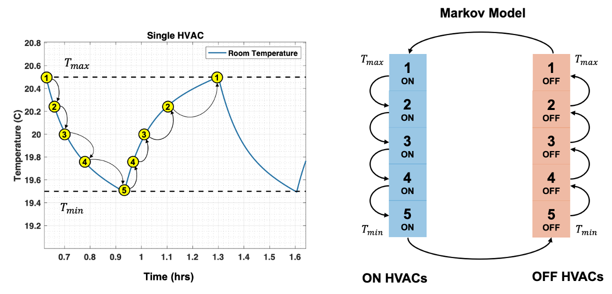
Next, the rate at which a TCL’s temperature transitions from one bin to the next is calculated or estimated, as illustrated in Fig 1. Fig 1 shows the case of air-conditioning loads, where TCLs transition from warmer to cooler bins when ON and cooler to warmer bins when OFF. The transition rates, for a given outdoor temperature, thermostat setpoint, and discrete-time step width $\Delta t$, are then populated into a $2N\times 2N$ matrix to form the transition rate matrix ($\Gamma$). Typically, the temperature dynamics of an individual TCL are considered in calculating the transition rates. Particularly in [10], the second-order TCL dynamics from (1) are considered, which characterizes both the indoor air and interior mass temperature dynamics. The resulting Markov chain model of aggregate TCL demand was shown to be more accurate than those based on a first-order simplified model. Hence, in this paper, we focus on the second order model representation for the Markov transition matrix. Please see [10, 13, 14] for more details on Markov chain modeling. Nevertheless, the methodology presented herein can be adapted to any Markov chain model of a TCL population. Thus, Markov chain model to capture aggregate TCL demand dynamics results in a discrete-time linear time-invariant (LTI) system model, as shown in (2):

$$x[k+1]=Ax[k],$$ (2)

where $x[k]\in\mathbb{R}^{2N}$ is a vector of the ON/OFF temperature bins. Furthermore, the value of an element $x_{i}[k]$ denotes the proportion of the population that is in the $i$-th bin at timestep $k$. Clearly, $\mathbf{1}_{2N}^{\top}x[k]=1$, i.e., the sum of all elements in $x[k]$ represents the entire population.

The system is autonomous and the population temperature distribution evolves based on the transition rate matrix the temperature setpoint, and the temperature deadband, which ensure correct switching dynamics at either boundary of the deadband. Note, that this paper considers TCL populations with homogeneous thermal parameters. However, heterogeneous populations can be characterized by either clustering the population into $K$ representative clusters and modeling each cluster as a homogeneous population [14] or leveraging historical or simulation data to estimate the $A$ matrix of a heterogeneous population [13]. The aggregate demand of the TCL population, $P_{\text{agg}}[k]$, represents the aggregate system’s output and can be calculated, as shown in (3),

$$P_{\text{agg}}[k] =c_{\text{ON}}x[k],$$ (3)

where $c_{\text{ON}}:=P_{\text{ON}}[\mathbf{1}^{\top}_{N}\leavevmode\nobreak\ \mathbf{0}_{N}^{\top}]$ and $P_{\text{ON}}>0$ is the total power capacity of the TCL fleet.

Next, we augment this model to characterize power output and temperature dynamics under setpoint control (i.e., the $T_{\text{set}}(t)$ can be modulated.

II-A TCL Thermostat Setpoint Control

In the case where TCL setpoints can be controlled, the population temperature distribution, $x[k]$, and by extension $P_{\text{agg}}[k]$ can be controlled. Therefore, the system is no longer autonomous and the evolution of $x[k]$ will depend on the setpoint change input. This is captured by separating the proportion of the TCL population that experienced a given setpoint change (actuated population) from the remainder of the population. Two state vectors are then defined, where $x_{a}[k]$ denotes the actuated population state vector and $x[k]$ denotes the rest of the population. The states $x[k]$ and $x_{a}[k]$ are governed by (4):

$$x[k+1] =A(x[k]-u[k]),$$ (4a)

$$x_{a}[k+1] =A_{\text{a}}(x_{a}[k]+u[k]),$$ (4b)

$$x[0]= x_{0},\quad x_{a}[0]=\mathbf{0}_{2N},$$ (4c)

where $u[k]\in\mathbb{R}^{2N}$ is the system input whose elements denote how much of the population at a particular bin will experience a setpoint change and is hence subtracted from $x[k]$ and the remainder of the population evolves naturally based on the system matrix $A$. The population that experienced a setpoint change is added to $x_{a}[k]$, which is initially zero, which then evolves naturally based on $A_{\text{a}}$ which is the actuated population system matrix. Fig 2 illustrates the evolution of the temperature distribution, and the corresponding aggregate demand of a TCL population wherein roughly 50% of the population experienced a setpoint change at $t=0$. The setpoint change was from 20^∘C to 22^∘C with the deadband ($\Delta T$) set to 1^∘C.

Figure 2: HVAC fleet temperature distribution (top) and aggregate power (bottom) evolution after setpoint change

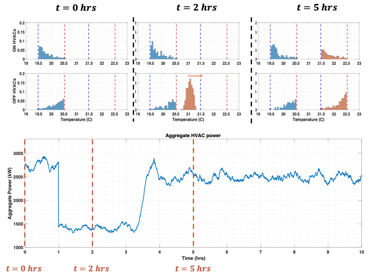
The aggregate power of the TCL fleet is calculated similarly to (3), where $P_{\text{agg}}[k]$ is just the sum of the ON proportion of the population. However, with setpoint control, there exists two ON populations due to $x_{a}[k]$ or $x[k]$. Therefore,

$$P_{\text{agg}}[k]=c_{\text{ON}}(x[k]+x_{a}[k]).$$ (5)

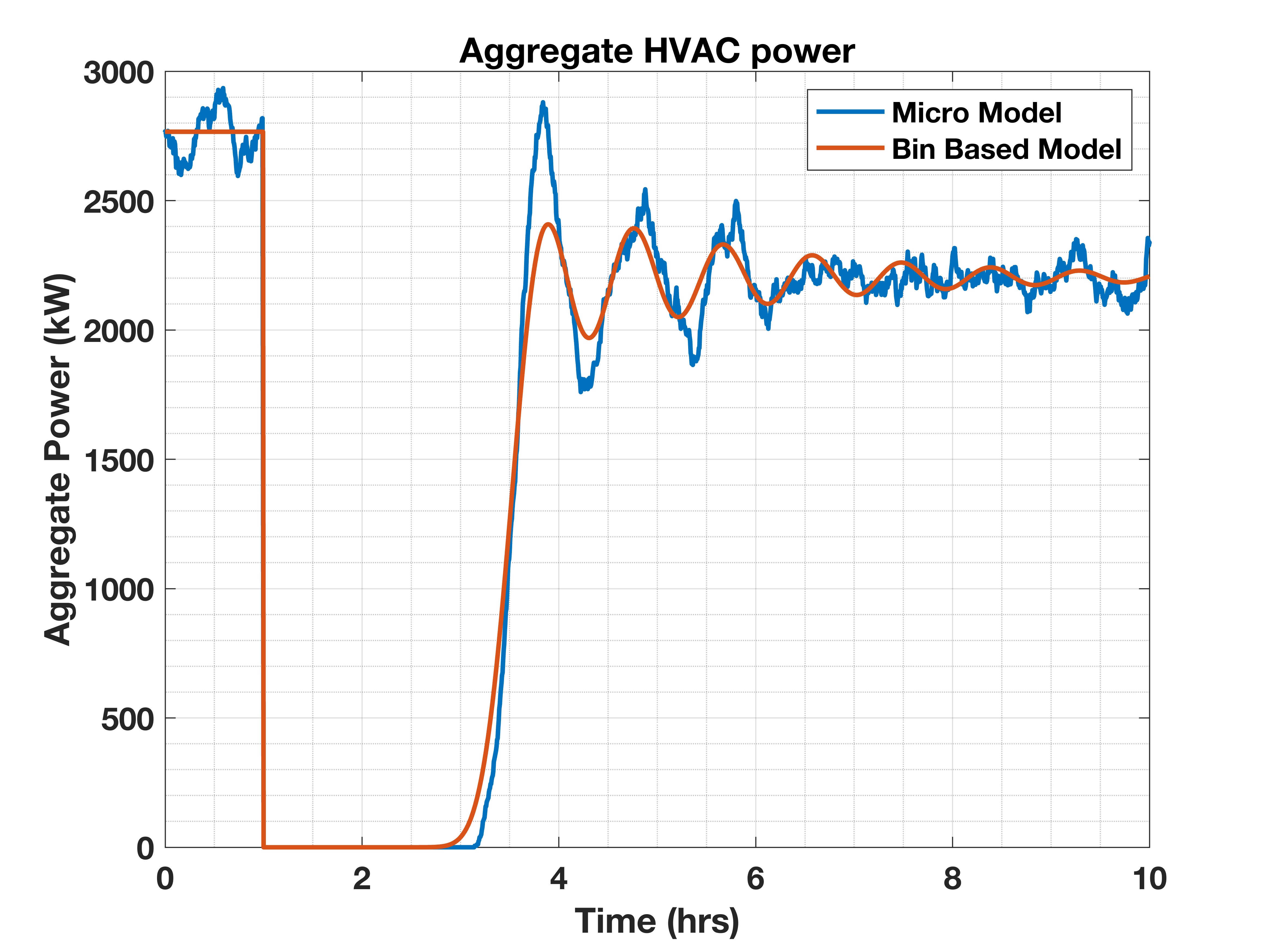
The discussed Markov chain aggregate TCL model is compared against an agent-based TCL simulation using the ETP model. Fig 3 shows the aggregate demand of a fleet of 1000 HVAC loads obtained both by the Markov chain aggregate model and the agent-based model following a setpoint change from 20^∘C to 22^∘C. Note that the agent based simulation considered a heterogeneous population whereas the Markov model considered a homogeneous population with the average parameter values of the heterogeneous population.

Figure 3: HVAC fleet aggregate power after setpoint change

Next, we present on the aggregate TCL model’s ability to characterize the reach-and-hold set.

III Reach and Hold Characterization

After defining and validating the aggregate TCL model, we now use it to identify the reach-and-hold set. The salient features of the reach-and-hold set are the change in power ($P_{\text{hold}}$) and the duration over which it can be sustained ($T_{\text{hold}}$). Thus, denote $P_{\text{hold}}$ to the lower bound on the change in aggregate power from the fleet’s nominal power consumption. Let $T_{\text{hold}}$ denote the minimum duration for which the aggregate demand change is held.

$\Delta P_{\text{agg}}[k]$ denotes the change in aggregate power of the TCL fleet from its nominal value at timestep $k$:

$$\Delta P_{\text{agg}}[k]=P_{\text{nom}}-P_{\text{agg}}[k]=P_{\text{nom}}-c_{\text{ON}}(x[k]+x_{a}[k]),$$ (6)

where $P_{\text{nom}}$ is the nominal aggregate power output of the fleet for a given $T_{\text{amb}}$ and defined analytically by the stationary distribution of the Markov chain model of the fleet (before any setpoint change). By recursively expressing $x[k]$ and $x_{a}[k]$ in terms of only the input, $u[k]$, and the initial conditions, $x[0]$ and $x_{a}[0]$, and substituting into (6), $\Delta P_{\text{agg}}[k]$ becomes

$$\Delta P_{\text{agg}}[k]=P_{\text{nom}}-c_{\text{ON}}\left(A^{k}x_{0}-\sum_{n=0}^{k-1}(A^{k-n}-A_{\text{a}}^{k-n})u[n]\right).$$ (7)

If the fleet is initially represented by its stationary distribution, $x_{0}$, then $A^{k}x_{0}=x_{0}$ and $P_{\text{agg}}[0]=P_{\text{nom}}=c_{\text{ON}}x_{0}$. This allows us to simplify (7) into

$$\Delta P_{\text{agg}}[k]=c_{\text{ON}}\sum_{n=0}^{k-1}(A^{k-n}-A_{\text{a}}^{k-n})u[n].$$ (8)

The reach and hold set is defined to be the largest $P_{\text{hold}}$ that can be realized such that $\Delta P_{\text{agg}}[k]\geq P_{\text{hold}}\forall k=1,2,\ldots,T_{\text{hold}}$. This can be formulated as a convex optimization problem as shown in (9):

$$\max_{u,P_{\text{hold}}}\quad P_{\text{hold}}$$ (9a)

s.t. $$\eqref{eqn: x_update}-\eqref{eqn: x_IC}$$ (9b)

$$\Delta P_{\text{agg}}[k] =c_{\text{ON}}\sum_{n=0}^{k-1}(A^{k-n}-A_{\text{a}}^{k-n})u[n]\geq P_{\text{hold}}\quad\forall k\leq T_{\text{hold}}$$ (9c)

$$u[k]\preceq x[k]\quad\forall k$$ (9d)

$$u[k]\succeq 0\quad\forall k$$ (9e)

Note that (9d) and (9e) are added to ensure an admissible control input. Also, without  (9d) and (9e) the problem becomes unbounded. Thus, for all $i$ elements and $k$ timesteps, $0\leq u_{i}[k]\leq x_{i}[k]$. Solving (9) for several values of $T_{\text{hold}}$ will characterize the reach and hold set of the TCL fleet. However, for a larger number of bins and/or larger time horizons, (9) becomes intractable. Therefore, we present a tractable inner approximation of the reach and hold set. Despite being an inner approximation, which under-estimates capability of a fleet, (i.e., is sub-optimal), it provides a guarantee on feasibility (i.e., any two-tuplet ($P_{\text{hold}},T_{\text{hold}})$ is achievable). To characterize the degree of conservativeness (suboptimality), we also present an outer approximation, which over-estimates the true reach-and-hold set and may include elements that are not achievable in (9).

III-A Inner Approximation of Reach and Hold Set

To find an inner approximation of the reach an hold set, it suffices to find a feasible solution to (9) with $P_{\text{hold}}\leq P^{*}_{\text{hold}}$, where $P^{*}_{\text{hold}}$ is the optimal $P_{\text{hold}}$ value of (9). This can then be repeated for several $T_{\text{hold}}$ values to form an inner approximation of the reach and hold set.

A feasible solution can be found by limiting the possible feasible values of $u[k]$ or by implementing a specific control policy. Consider the following uniformly proportional bin control policy

$$u[k]=\alpha[n]\leavevmode\nobreak\ x_{0},$$ (10)

where $\alpha[n]\in\mathbb{R}$. The setpoint change control input $u[k]$ is limited to be a scalar multiple of the initial population distribution which is assumed to be a steady-state distribution ($A^{k}x_{0}=x_{0}\forall k$). This reduces the number of variables by a factor of $2N$. Originally, solving for $u[k]\in\mathbb{R}^{2N}$ involves solving $2N$ variables every timestep. On the other hand, with (10) imposed, a scalar variable needs to be solved for every timestep.

Substituting (10) into (9), yields the following optimization problem:

$$\max_{\alpha_{i},P_{\text{hold}}}\quad P_{\text{hold}}$$ (11a)

s.t. $$\sum_{n=0}^{k-1}\alpha[n](P_{\text{nom}}-c_{\text{ON}}A_{\text{a}}^{k-n}x_{0})\geq P_{\text{hold}}\quad\forall k\leq T_{\text{hold}}$$ (11b)

$$\alpha[k]\geq 0\quad\forall k$$ (11c)

$$\sum_{k=0}^{T_{\text{hold}}-1}\alpha[k]\leq 1\quad$$ (11d)

Remark (Thermostat Setpoint Change).

If the change in thermostat setpoint from $T_{\text{set}}$ to $T_{\text{set}}^{\text{new}}$ ($T_{\text{set}}^{\text{new}}-T_{\text{set}}=\Delta T_{\text{set}}$) is such that $\Delta T_{\text{set}}\geq\Delta T$, where $\Delta T$ is the thermostat deadband. Then $C_{\text{ON}}A_{\text{a}}x_{0}=0$ since all non-zero elements in $x_{0}$ will correspond to temperature bins that are lower than $T_{\text{set}}-\frac{\Delta T}{2}$ causing the population to transition to their corresponding OFF bins. In other words, all the non-zero elements $A_{\text{a}}x_{0}$ will be in OFF bins and, hence, $C_{\text{ON}}A_{\text{a}}x_{0}=0$.

For a setpoint change $\Delta T_{\text{set}}\geq\Delta T$, (11b) is reduced to

$$\alpha[k]\geq\alpha_{\text{LB}}[k],$$ (12)

where

$$\alpha_{\text{LB}}[k]:=\begin{cases}\frac{P_{\text{hold}}}{P_{\text{nom}}}&\text{if }k=0\\ \\ \frac{P_{\text{hold}}}{P_{\text{nom}}}+\sum_{n=0}^{k-1}\alpha[n](-1+\frac{c_{\text{ON}}}{P_{\text{nom}}}A^{k-n+1}_{a}x_{0})&\text{if }k\geq 1\end{cases}.$$ (13)

Note that we assume here that $P_{\text{nom}}>0$. Using (12) and (13) and given a value of $P_{\text{hold}}$, a feasible $\{P_{\text{hold}},T_{\text{hold\}}}$ pair can be found. This is achieved by recursively choosing $\alpha[k]=\max\{\alpha_{\text{LB}}[k],0\}$ for a given value of $P_{\text{hold}}$. By doing so, $\Delta P_{\text{agg}}[k]\geq P_{\text{hold}}$ is guaranteed. The value of $T_{\text{hold}}$ is then found by propagating $\alpha[k]=\max\{\alpha_{\text{LB}}[k],0\}$ forward in time until $\sum_{\forall k}\alpha[k]\geq 1$. The value of $\alpha[k]$ for any future timesteps is set to zero. Lastly, $\Delta P_{\text{agg}}[k]$ is propagated forward with $T_{\text{hold}}$ being the last timestep beyond which $\Delta P_{\text{agg}}[k]<P_{\text{hold}}$. The resulting $\{P_{\text{hold}},T_{\text{hold}}\}$ pair and their corresponding values of $\alpha[k]$ satisfy all constraints in (11) and therefore, $\{P_{\text{hold}},T_{\text{hold}}\}$ is a feasible pair. This procedure is summarized in Algorithm 1.

Algorithm 1 Reach and Hold Set Inner Approximation

1:Initialize: $P_{\text{hold}}\in[0,P_{\text{nom}}]$

2:Initialize: $T_{\max}$

3:for all $k=0,\ldots,T_{\text{max}}$ do

4:     $\alpha[k]=\max\{\alpha_{\text{LB}}[k],0\}$

5:     $T_{d}=k$

6:     if $\sum_{n=0}^{k}\alpha[k]\geq 1$ then

7:         $\alpha[k]=\alpha[k]-(\sum_{n=0}^{k}\alpha[k]-1)$

8:         break

9:     end if

10:end for

11:for all $k=T_{d}+1,\ldots,T_{\text{max}}$ do

12:     $\alpha[k]=0$

13:     if $\sum_{n=0}^{k-1}\alpha[n](P_{\text{nom}}-c_{\text{ON}}A_{\text{a}}^{k-n}x_{0})<P_{\text{hold}}$ then

14:         $T_{\text{hold}}=k-1$

15:     else

16:         $T_{\text{hold}}=k$

17:     end if

18:end for

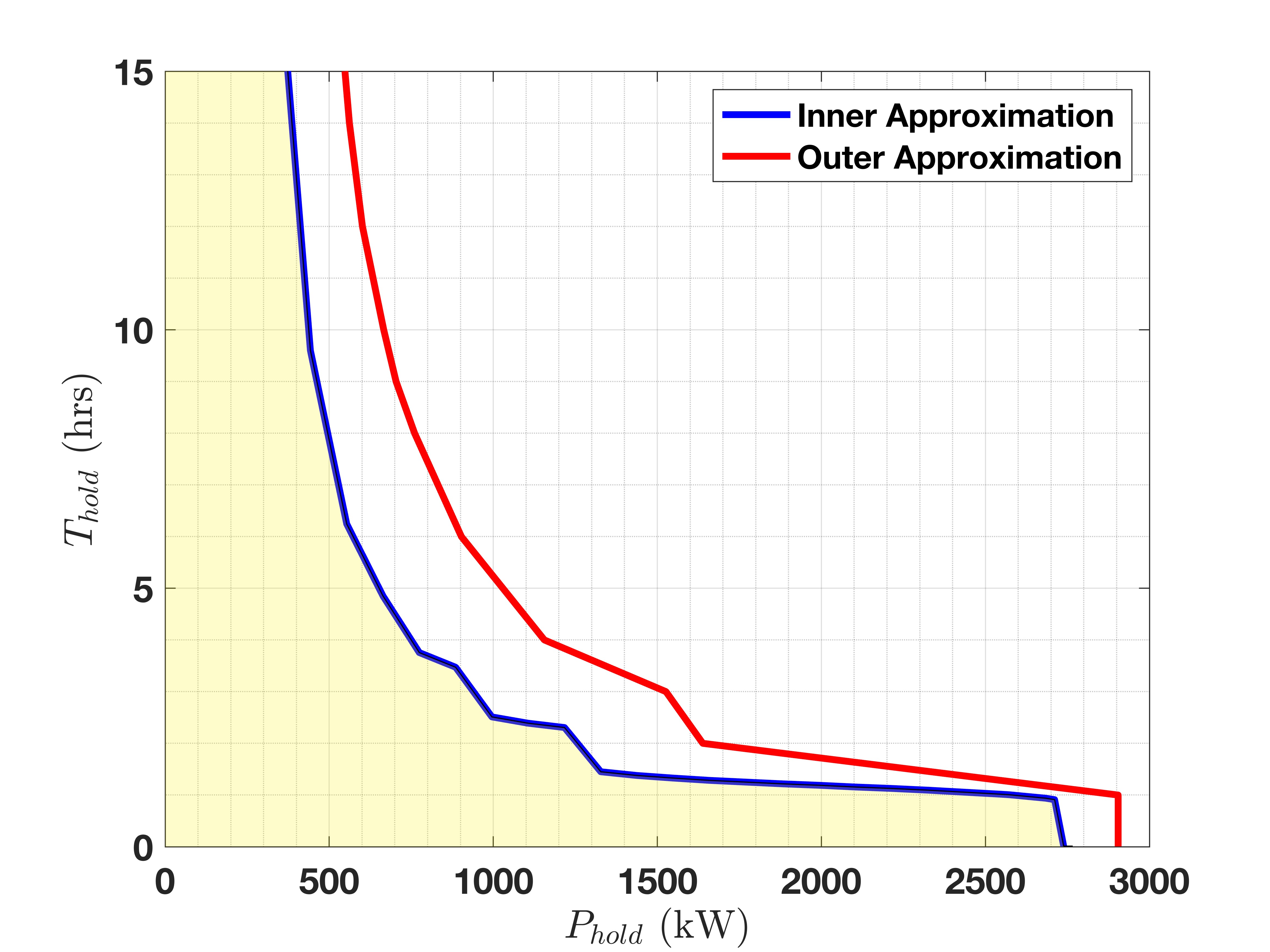
The procedure outlined in Algorithm 1 is repeated for several $P_{\text{hold}}$ values. The obtained $\{P_{\text{hold}},T_{\text{hold}}\}$ pairs define the boundary of the reach and hold inner approximation and are plotted in Fig 4 (blue line). Let $\mathcal{R}_{\text{in}}\subseteq\mathcal{R}$ denote the inner approximation to reach and hold set inner approximation. $\mathcal{R}_{\text{in}}$ is shown in Fig 4 as the yellow-shaded region (inclusive of the boundary).

Figure 4: Reach and hold set of TCL population, inner approximation (blue) and outer approximation (red)

III-B Outer Approximation of Reach and Hold Set

An outer approximation of the true reach and hold set is identified next. The true reach and hold set will satisfy $\mathcal{R}_{\text{in}}\subseteq\mathcal{R}\subseteq\mathcal{R}_{\text{out}}$. Although an $\mathcal{R}_{\text{in}}$ can include infeasible $\{P_{\text{hold}},T_{\text{hold}}\}$ pairs, it can be used to assess the sub-optimality of the inner approximation.

To identify $\mathcal{R}_{\text{out}}$, a fictitious system is defined wherein the population temperature state is pushed towards the lower temperature bound $T_{\text{set}}-\frac{\Delta T}{2}$. This can be achieved by adjusting the initial setpoint temperature to be $T_{\text{set}}-\frac{\Delta T}{2}$ and adjusting the temperature deadband equal to the temperature difference between two consecutive bins. Such a system ’squeezes’ the population’s temperature distribution into a significantly smaller number of bins (lower variance). Since $u_{i}[k]\leq x_{i}[k]$ for all bins $i$, most of the elements of $u[k]$ will be forced to zero. This is then used to eliminate a significant number of variables from the optimization problem.

Let $A_{\text{out}}$ denote the system matrix of the fictional system discussed. The optimization formulation used to characterize an outer approximation of the reach and hold set is then

$$\max_{\bar{u},\bar{P}_{\text{hold}}}\quad \bar{P}_{\text{hold}}$$ (14a)

s.t. $$\sum_{n=0}^{k-1}c_{\text{ON}}(A_{\text{out}}^{k-n}-A_{\text{a}}^{k-n})\bar{u}[n]\geq\bar{P}_{\text{hold}}\quad\forall k\leq T_{\text{hold}}$$ (14b)

$$\bar{u}[k]\succeq 0\quad\forall k$$ (14c)

$$\sum_{k=0}^{T_{\text{hold}}-1}\mathbf{1}^{T}\bar{u}[k]\leq 1\quad$$ (14d)

where $\bar{u}[k]$ is the control input to the fictitious system and $\bar{P}_{\text{hold}}$ is the outer approximation of $P_{\text{hold}}$ for a given value of $T_{\text{hold}}$. Comparing (14) to the original problem (9), (14b) is similar to (9c) but with $A_{\text{out}}$ instead of $A$. Furthermore, the constraint (9d) is relaxed and replaced with the (14d), which was implicitly enforced by (9d) in (9). The intuition behind choosing this fictitious system was that for lower temperature bins, ON bins have lower transition rates/probabilities, and the opposite for OFF bins. In other words, the probability of transitioning out of the ON bins is lower. By squeezing the population into the lower temperature bins, the k-step transition probability to an ON bin would be larger ($c_{\text{ON}}(A_{\text{out}}^{k-n}\bar{u}[n]\geq c_{\text{ON}}(A^{k-n}\bar{u}[n])$). This expands the set of feasible $P_{\text{hold}}$ values compared to the original problem (outer approximation). This outer approximation is discussed next.

III-B1 Guarantees on outer approximation

We are interested in understanding, if given a value of $T_{\text{hold}}$, for every feasible $u[k]$ of (9) is there an equivalent feasible $\bar{u}[k]$ in (14) that will result in $\bar{P}_{\text{hold}}\geq P_{\text{hold}}$ at optimality? If so, then the set of feasible $\bar{P}_{\text{hold}}$ in (14) is larger than that of (9).

To answer this, let $\Xi_{\text{hold}}$ and $\Xi_{\text{hold}}^{\text{outer}}$ be sets of feasible $P_{\text{hold}}$ values of (9) and (14), respectfully, for fixed $T_{\text{hold}}$. A mapping between $\bar{u}[k]$ and $u[k]$ can be shown as (15):

$$\bar{u}[k]=x_{\text{out}}(\mathbf{1}_{2N}^{T}u[k]),$$ (15)

where $x_{\text{out}}\in\mathbb{R}^{2N}$ is a vector with all zeros, except for a 1 at bin $(T_{\text{set}}-\frac{\Delta T}{2})$. Let $h_{k},h_{\text{a},k},h_{\text{out},k}\in\mathbb{R}^{2N}$ be defined as

$$h_{k}^{T} =c_{\text{ON}}A^{k}$$ (16a)

$$h_{\text{a},k}^{T} =c_{\text{ON}}A_{\text{a}}^{k}$$ (16b)

$$h_{\text{out},k}^{T} =c_{\text{ON}}A_{\text{out}}^{k}.$$ (16c)

With that, (9c) and (14b) can be re-written

$$\sum_{n=0}^{k-1}(h_{k-n}^{T}-h_{\text{a},k-n}^{T})u[n]\geq P_{\text{hold}}\quad\forall k\leq T_{\text{hold}}$$ (17a)

$$\sum_{n=0}^{k-1}(h_{\text{out},k-n}^{T}-h_{\text{a},k-n}^{T})\bar{u}[n]\geq\bar{P}_{\text{hold}}\quad\forall k\leq T_{\text{hold}}$$ (17b)

Also, let $(h_{\text{out},k-n}^{T}-h_{\text{a},k-n}^{T})x_{\text{out}}=h_{k-n}^{x}\in\mathbb{R}$ .

Proposition 1.

If $h_{k-n}^{x}\mathbf{1}_{2N}\succeq(h_{k-n}-h_{\text{a},k-n})\quad\forall k\leq T_{\text{hold}}\text{ and }\forall n\leq k$, then the reach and hold set characterized by formulation (14) is an outer approximation of the actual reach and hold set characterized using (9).

Proof.

Let $u[k]$ be an optimal solution and $P_{\text{hold}}$ be the corresponding optimal objective of (9). Since $u[k]$ satisfies (9e), given the mapping shown in (15), $\bar{u}[k]$ satisfies (14c). To show that $\bar{u}[k]$ satisfies (14d), (18) is first obtained by expressing $x[k]$ in (9d) in terms of the input $u[k]$ and the initial condition $x_{0}$.

$$u[k]\succeq A^{k}x_{0}-\sum_{n=0}^{k-1}A^{k-n}u[n]$$ (18)

Multiplying both sides of (18) by $\mathbf{1}_{2N}^{T}$ and substituting $\mathbf{1}_{2N}^{T}A=\mathbf{1}_{2N}^{T}$ since the columns of $A$ sum up to 1, (19) is obtained.

$$\sum_{n=0}^{k}\mathbf{1}_{2N}^{T}u[n]\leq\mathbf{1}_{2N}^{T}x_{0}=1$$ (19)

Since (19) holds then $\bar{u}[k]$ satisfies (14d). Therefore, $\bar{u}[k]$ is feasible in (14).

Now, let $\Delta P[k]$ and $\Delta P_{\text{out}}[k]$ denote the left-hand side of the expressions in (17a) and (17b) respectively at timestep $k$.

By substituting (15) into (17b), (20) is obtained:

$$\Delta P_{\text{out}}[k]=\sum_{n=0}^{k-1}(h_{\text{out},k-n}^{T}-h_{\text{a},k-n}^{T})x_{\text{out}}(\mathbf{1}_{2N}^{T}u[n])\geq\bar{P}_{\text{hold}}.$$ (20)

The expression in (20) can be further simplified into (21)

$$\Delta P_{\text{out}}[k]=\sum_{n=0}^{k-1}\ (h_{k-n}^{x}\mathbf{1}_{2N}^{T})u[n]\geq\bar{P}_{\text{hold}}.$$ (21)

Comparing (17a) and (21), if $(h_{k-n}^{x}\mathbf{1}_{2N}^{T})\succeq(h_{k-n}-h_{\text{a},k-n})$ holds, then (22) also must hold.

$$\Delta P_{\text{out}}[k]\geq\Delta P[k]\quad\forall k\leq T_{\text{hold}}$$ (22)

At optimality, at least one timestep exists wherein (17a) and (17b) are strict ($\Delta P_{\text{out}}[k]=\bar{P}_{\text{hold}}$ and $\Delta P=P_{\text{hold}}$) . Otherwise, $P_{\text{hold}}$ and/or $\bar{P}_{\text{hold}}$ can be increased (improving optimality) without violating any constraints. Then if (22) holds, that implies $\bar{P}_{\text{hold}}\geq P_{\text{hold}}$. Therefore, for every optimal $u[k]$ of (9), there exists a $\bar{u}[k]$ and corresponding $\bar{P}_{\text{hold}}$ such that $\bar{P}_{\text{hold}}\geq P_{\text{hold}}$. Furthermore, $P_{\text{hold}}$ is the respective upper extreme of $\Xi_{\text{hold}}$ and $\bar{P}_{\text{hold}}$ is a lower bound on the upper extreme of $\Xi_{\text{hold}}^{\text{outer}}$ since $\bar{P}_{\text{hold}}$ is a feasible point of (14) . The lower extreme of both is $\Xi_{\text{hold}}$ and $\Xi_{\text{hold}}^{\text{outer}}$ is zero. Hence $\Xi_{\text{hold}}=[0,P_{\text{hold}}]\subseteq[0,\bar{P}_{\text{hold}}]\subseteq\Xi_{\text{hold}}^{\text{outer}}$. Since the feasible set $\Xi_{\text{hold}}$ is a subset of $\Xi_{\text{hold}}^{\text{outer}}$, the reach and hold set characterized using (14) is an outer approximation of the reach and hold set.  ∎∎

The element-wise inequality $h_{k-n}^{x}\mathbf{1}_{2N}\succeq(h_{k-n}-h_{\text{a},k-n})\quad\forall k,n\leq T_{\text{hold}}$ cannot be checked analytically (as far as authors are aware), but represents a key condition, which can be checked empirically for a given system.

This condition was checked and verified empirically. Fig 4 shows the outer approximation obtained using the optimization problem formulated in (14). Thus, the inner approximation provides a realizable reach and hold set for a HVAC fleet and from the outer approximation, we can determine worst-case conservativeness of the inner approximation.

III-C Aggregating Reach and Hold Sets

When two or more populations of TCLs are present. The reach and hold set of each group can be found separately, and from that, the reach and hold set of both populations combined can be found.

Let $(P^{1}_{\text{hold}},T^{1}_{\text{hold}})$ be a feasible point in the reach and hold set of the first population. This implies that there exists a control input trajectory such that $\Delta P^{1}_{\text{agg}}[k]\geq P^{1}_{\text{hold}}\quad\forall k=1,\dots,T^{1}_{\text{hold}}$. Also, let $(P^{2}_{\text{hold}},T^{2}_{\text{hold}})$ be feasible point in the reach and hold set of the second population. The aggregation of the points $(P^{1}_{\text{hold}},T^{1}_{\text{hold}})$ and $(P^{2}_{\text{hold}},T^{2}_{\text{hold}})$ is first considered before moving on to the aggregation of the reach and hold set.

Let the total change in power trajectory of the two populations be denoted $\Delta P^{12}_{\text{agg}}[k]$ and, let $P^{12}_{\text{hold}}$ and $T^{12}_{\text{hold}}$ be feasible reach and hold pair of the combined population. $\Delta P^{12}_{\text{agg}}[k]$ will consist of some combination $\Delta P^{1}_{\text{agg}}[k]\text{ and }\Delta P^{2}_{\text{agg}}[k]$ as shown in (23).

$$\Delta P^{12}_{\text{agg}}[k]=\Delta P^{1}_{\text{agg}}[k]+\Delta P^{2}_{\text{agg}}[k+\tau]\geq P^{12}_{\text{hold}}\quad\forall k\leq T^{12}_{\text{hold}},$$ (23)

where $\tau$ is the time lag between depending on when the first and second control trajectories are applied. The control trajectories of the individual populations can be applied in one of three ways, either 1) exclusively (only one of the populations is actuated), 2) simultaneously ($\tau=0$), or 3) consecutively ($|\tau|>0$). Fig 5 shows a (simplified) illustration of simultaneous and consecutive actuations of the populations with the green line showing the total change in aggregate power $\Delta P^{12}_{\text{agg}}[k]$ versus time (. From Fig 5, four possible reach and hold sets from the aggregation of $(P^{1}_{\text{hold}},T^{1}_{\text{hold}})$ and $(P^{2}_{\text{hold}},T^{2}_{\text{hold}})$ can be identified and are shown in (24)

$$P^{12}_{\text{hold}}\in[0,P^{1}_{\text{hold}}],\quad T^{12}_{\text{hold}}\in[0,T^{1}_{\text{hold}}]$$ (24a)

$$P^{12}_{\text{hold}}\in[0,P^{2}_{\text{hold}}],\quad T^{12}_{\text{hold}}\in[0,T^{2}_{\text{hold}}]$$ (24b)

$$P^{12}_{\text{hold}}\in[0,P^{1}_{\text{hold}}+P^{2}_{\text{hold}}],\quad T^{12}_{\text{hold}}\in[0,\min\{T^{1}_{\text{hold}},T^{2}_{\text{hold}}\}]$$ (24c)

$$P^{12}_{\text{hold}}\in[0,\min\{P^{1}_{\text{hold}},P^{2}_{\text{hold}}\}],\quad T^{12}_{\text{hold}}\in[0,T^{1}_{\text{hold}}+T^{2}_{\text{hold}}]$$ (24d)

Figure 5: Change in aggregate demand caused by two TCL fleets. Simultaneous actuation of both populations (left) and consecutive actuation (right).

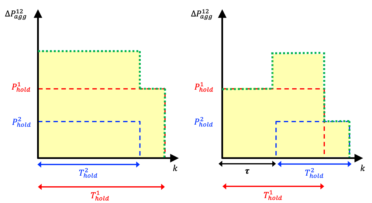
with (24a) and (24b) being the possible reach and hold values if only one of the two populations were to be actuated. (24c) describes the possible reach and hold values when both populations are actuated simultaneously and (24d) is the same when both populations are actuated consecutively. All other possible reach are hold points have to be subsets of either of (24a)-(24d) and the overall reach and hold set would be the union of (24a)-(24d).

For a given value $T_{\text{hold}}=t$, let the corresponding maximum $P_{\text{hold}}$ values of the individual populations be $P^{1}_{\text{hold,t}}$ and $P^{2}_{\text{hold,t}}$ respectively. Similarly, for a given value $P_{\text{hold}}=p$, let the corresponding maximum $T_{\text{hold}}$ values of the individual populations be $T^{1}_{\text{hold,p}}$ and $T^{2}_{\text{hold,p}}$ respectively.

III-C1 Exclusive Actuation

In the case when only one of the populations is actuated, for required $T^{12}_{\text{hold}}=t$, the set $\mathcal{P}^{12}_{\text{ex,t}}\in[0,\max\{P^{1}_{\text{hold,t}},P^{2}_{\text{hold,t}}\}]$ will encompass all feasible $P_{\text{hold}}$ values that can be achieved with $T^{12}_{\text{hold}}=t$. This can be done for several values of $t$ to define the set $\mathcal{P}^{12}_{\text{ex}}$.

III-C2 Simultaneous Actuation

For the simultaneous case, where $\tau=0$, the corresponding $P^{12}_{\text{hold}}$ and $T^{12}_{\text{hold}}$ are shown in (24c). From (24c) it is clear that if we require $T^{12}_{\text{hold}}=t$ then both $T^{1}_{\text{hold}}\geq t$ and $T^{2}_{\text{hold}}\geq t$ need to hold. Also, $P_{\text{hold}}$ increases as $T_{\text{hold}}$ decreases as seen in Fig 4. Therefore, $P^{1}_{\text{hold}}=P^{1}_{\text{hold,t}}$ and $P^{2}_{\text{hold}}=P^{2}_{\text{hold,t}}$ are maximum values of $P^{1}_{\text{hold}}$ and $P^{2}_{\text{hold}}$. Hence, the set $\mathcal{P}^{12}_{\text{sim}}\in[0,P^{1}_{\text{hold,t}}+P^{2}_{\text{hold,t}}]$ will encompass all feasible $P_{\text{hold}}$ values that can be achieved with $T^{12}_{\text{hold}}=t$. This can be done for several values of $t$ to define the set $\mathcal{P}^{12}_{\text{sim}}$.

III-C3 Consecutive Actuation

For the consecutive case, where $\tau>0$, the corresponding $P^{12}_{\text{hold}}$ and $T^{12}_{\text{hold}}$ are shown in (24d). Similar to the consecutive case, if we require $P^{12}_{\text{hold}}=p$ then both $P^{1}_{\text{hold}}\geq p$ and $P^{2}_{\text{hold}}\geq p$ need to hold. Also, $T_{\text{hold}}$ increases as $P_{\text{hold}}$ decreases as seen in Fig 4. Therefore, $T^{1}_{\text{hold}}=T^{1}_{\text{hold,p}}$ and $T^{2}_{\text{hold}}=T^{2}_{\text{hold,p}}$ are maximum values of $T^{1}_{\text{hold}}$ and $T^{2}_{\text{hold}}$. Hence, the set $\mathcal{T}^{12}_{\text{con,p}}\in[0,T^{1}_{\text{hold,t}}+T^{2}_{\text{hold,t}}]$ will encompass all feasible $T_{\text{hold}}$ values that can be achieved with $P^{12}_{\text{hold}}=p$. This can be done for several values of $t$ to define the set $\mathcal{T}^{12}_{\text{con}}$.

Now, the overall reach and hold set can be expressed as the union of $\mathcal{P}^{12}_{\text{ex}}$, $\mathcal{P}^{12}_{\text{sim}}$ and $\mathcal{T}^{12}_{\text{con}}$.

III-D Effect of $\Delta T_{\text{set}}$ on Reach and hold set

Figure 6: Effect of setpoint change ($\Delta T_{\text{set}}$) on reach and hold set

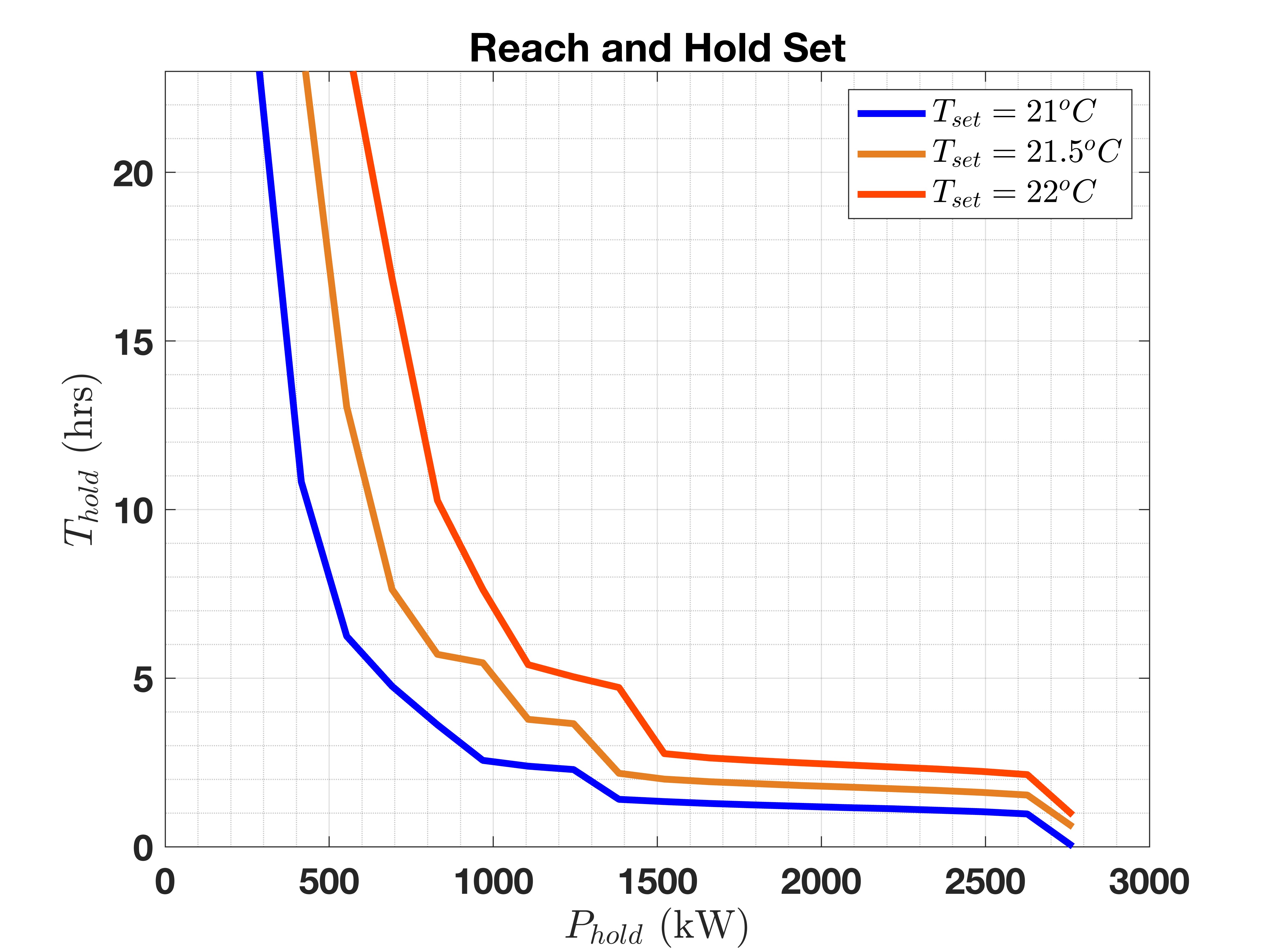
The characterized reach and hold set is dependent on the change in setpoint temperature. To illustrate this, the reach and hold set of a fleet of TCLs is characterized with a starting setpoint temperature of 20^∘C and a new setpoint temperature of 21^∘ C, 21.5^∘C and 22^∘C respectively. Fig 6 shows the respective reach and hold sets (inner approximations). Fig 6 shows that as the new setpoint temperature increases, so do the values of $T_{\text{hold}}$ since it takes a longer time for the TCLs to reach the new upper limit temperature ($T^{\text{new}}_{\text{set}}+\frac{\Delta T}{2})$ for larger setpoint changes.

III-E Effect of pre-cooling on reach and hold set

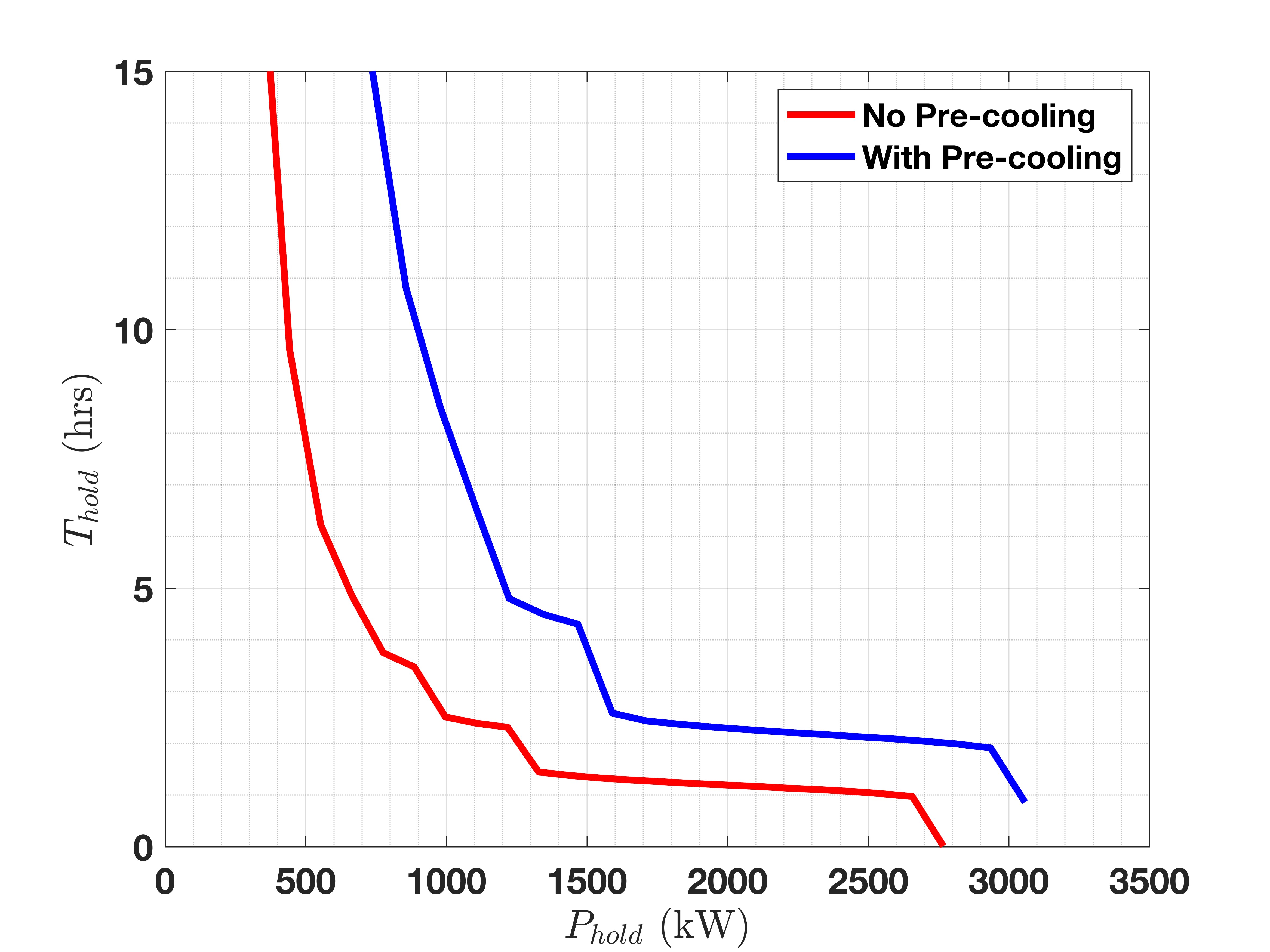
A common occurrence in DR schemes in an attempt to maintain user comfort is that the fleet can be pre-cooled to a lower temperature before demand response occurs. Thus allowing for longer $T_{\text{hold}}$ durations for the same level of user discomfort or for the same $T_{\text{set}}^{\text{new}}$. Fig 7 shows two reach and hold sets of the same TCL fleet. However, once with a starting temperature of 20^∘ and the other with a ’pre-cooled’ starting temperature of 19^∘. Fig 7 shows that pre-cooling has an effect on both $P_{\text{hold}}$ and $T_{\text{hold}}$. Since, pre-cooling increases the temperature distance between the TCL device temperatures and the new upper limit temperature after the setpoint change and hence increasing $T_{\text{hold}}$. Furthermore, since the population was initially kept at a cooler temperature in the pre-cooled case, the nominal aggregate power consumption was larger than in the case without pre-cooling. Therefore, this allowed for larger $P_{\text{hold}}$ values that were previously infeasible.

Figure 7: Effect of pre-cooling on reach and hold set

IV Simulation Results

Figure 8: Micro model validation of reach and hold set

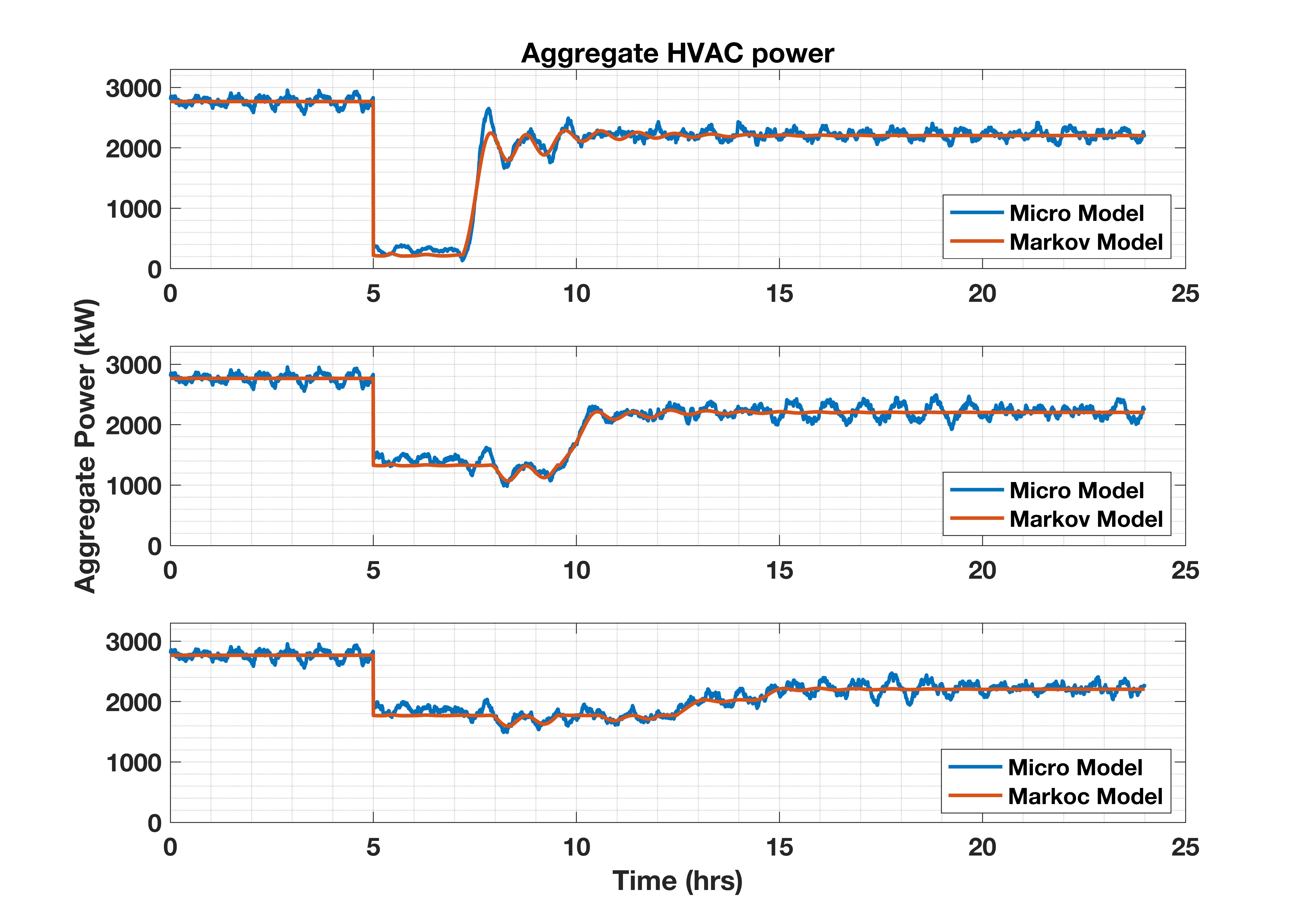
The characterized reach and hold set uses a Markov chain model to capture the aggregate power dynamics of a TCL population. However, as illustrated in Fig 3 there is some discrepancies between the Markov Chain model and modeling each TCL individually using the ETP model. Therefore, the values of $u[k]$ obtained while finding the inner approximation of the reach and hold set were also applied to the micro-simulation. The resulting aggregate power of both the Markov model and micro model is then compared.

The obtained control input $u[k]$ was applied to the micro-simulation such that the number of TCL units that experience a setpoint change is roughly the same as in the Markov model. This can be found by summing all the elements of $u[k]$ and scaling by the number of TCLs in the micro-simulation ($N_{\text{TCL}}$). However, there is no guarantee that $N_{\text{TCL}}\mathbf{1}^{T}u[k]$ takes an integer value. Therefore, $u[k]$ cannot be applied directly, and some post-processing is necessary as shown next:

$$U[k] =N_{\text{TCL}}u[k]$$ (25a)

$$\hat{u}[k] =\lfloor U[k]+e[k]\rfloor$$ (25b)

$$e[k+1] =u[k]-\hat{u}[k]$$ (25c)

$$e[0] =0,$$ (25d)

where $\hat{u}[k]$ is the control input that is applied to the micro-simulation of the TCLs. $e[k]$ is the error accrued in the last timestep due to flooring the control input $u[k]$ to the closest integer value. The error is carried forward and in an attempt to reduce the discrepancy between $\hat{u}[k]$ and $u[k]$. Fig 8 shows the aggregate power of the TCL fleet both from the micro-simulation and the Markov model for an approximately 2-hr, 4-hr and 8-hr DR block with a setpoint change from 20^∘C to 22^∘C. Fig 8 shows despite some discrepancies due to the flooring of the input the micro model simulation resulted in approximately the same reach and hold behavior.

V CONCLUSION

This paper provides a methodology for analyzing and computing the capacity of fleets of TCLs to participate in demand response events. The capacity is represented by the fleet’s ability to deviate from nominal (change in power) and the duration for which it can hold this deviation (time interval). We denote this the reach-and-hold set and present an optimization-based methodology for finding the set. However, the formulation is intractable for practical cases, so we provide a simplified formulation that represents inner (computational) and outer (analytical) approximations of the reach-and-hold set and show empirically that these approximations are potentially useful. Future work will tighten the approximations and provide analytical bounds on optimality gap, as well as, adapting the methodology to different load types and consider how the sets evolve dynamically to characterize flexibility more completely. Lastly, we seek to understand the role of different control methodologies in shaping the reach-and-hold sets and general flexibility.

References

- [1] A.. Annaswamy, K.. Johansson and G.. Pappas “Control for Societal-scale Challenges: Road Map 2030” Accessed: 2024-03-22, IEEE Control Systems Society Publication, 2023 URL: https://ieeecss.org/control-societal-scale-challenges-roadmap-2030
- [2] Mads R. Almassalkhi and Soumya Kundu “Intelligent Electrification as an Enabler of Clean Energy and Decarbonization” In Current Sustainable/Renewable Energy Reports 10, 2023
- [3] Rick Davis “What is Tesla’s Virtual Power Plant?”, 2023 LastBulb URL: https://www.lastbulb.com/virtual-power-plant
- [4] Jennifer Downing et al. “Pathways to Commercial Liftoff: Virtual Power Plants”, 2023 URL: https://liftoff.energy.gov/wp-content/uploads/2023/10/LIFTOFF_DOE_VVP_10062023_v4.pdf
- [5] Peter Alstone and al. “2025 California Demand Response Potential Study – Charting California’s Demand Response Future”, 2017
- [6] He Hao, Borhan M. Sanandaji, Kameshwar Poolla and Tyrone L. Vincent “Aggregate Flexibility of Thermostatically Controlled Loads” In IEEE Transactions on Power Systems 30.1, 2015, pp. 189–198 DOI: 10.1109/TPWRS.2014.2328865
- [7] Oluwagbemileke Oyefeso et al. “Control of Aggregate Air-Conditioning Load using Packetized Energy Concepts”, 2022, pp. 7
- [8] Emilio Benenati, Marcello Colombino and Emiliano Dall’Anese “A tractable formulation for multi-period linearized optimal power flow in presence of thermostatically controlled loads” In 2019 IEEE 58th Conference on Decision and Control (CDC), 2019, pp. 4189–4194 DOI: 10.1109/CDC40024.2019.9030029
- [9] Samuel Cordova, Claudio A. Canizares, Alvaro Lorca and Daniel E. Olivares “Aggregate Modeling of Thermostatically Controlled Loads for Microgrid Energy Management Systems” In IEEE Transactions on Smart Grid 14.6, 2023, pp. 4169–4181 DOI: 10.1109/TSG.2023.3254655
- [10] Wei Zhang, Jianming Lian, Chin-Yao Chang and Karanjit Kalsi “Aggregated Modeling and Control of Air Conditioning Loads for Demand Response” In IEEE Transactions on Power Systems 28.4, 2013, pp. 4655–4664 DOI: 10.1109/TPWRS.2013.2266121
- [11] Saeid Bashash and Hosam K. Fathy “Modeling and Control of Aggregate Air Conditioning Loads for Robust Renewable Power Management” In IEEE Transactions on Control Systems Technology 21.4, 2013, pp. 1318–1327 DOI: 10.1109/TCST.2012.2204261
- [12] Jun Zheng, Gabriel Laparra, Guchuan Zhu and Meng Li “Aggregate Power Control of Heterogeneous TCL Populations Governed by Fokker–Planck Equations” In IEEE Transactions on Control Systems Technology 28.5, 2020, pp. 1915–1927 DOI: 10.1109/TCST.2020.2968873
- [13] Johanna L. Mathieu, Stephan Koch and Duncan S. Callaway “State Estimation and Control of Electric Loads to Manage Real-Time Energy Imbalance” In IEEE Transactions on Power Systems 28.1, 2013, pp. 430–440 DOI: 10.1109/TPWRS.2012.2204074
- [14] Md Salman Nazir and Ian A. Hiskens “Noise and Parameter Heterogeneity in Aggregate Models of Thermostatically Controlled Loads” 20th IFAC World Congress In IFAC-PapersOnLine 50.1, 2017, pp. 8888–8894 DOI: https://doi.org/10.1016/j.ifacol.2017.08.1547