Failures and Successes of Cross-Validation for
Early-Stopped Gradient Descent

Abstract

We analyze the statistical properties of generalized cross-validation (GCV) and leave-one-out cross-validation (LOOCV) applied to early-stopped gradient descent (GD) in high-dimensional least squares regression. We prove that GCV is generically inconsistent as an estimator of the prediction risk of early-stopped GD, even for a well-specified linear model with isotropic features. In contrast, we show that LOOCV converges uniformly along the GD trajectory to the prediction risk. Our theory requires only mild assumptions on the data distribution and does not require the underlying regression function to be linear. Furthermore, by leveraging the individual LOOCV errors, we construct consistent estimators for the entire prediction error distribution along the GD trajectory and consistent estimators for a wide class of error functionals. This in particular enables the construction of pathwise prediction intervals based on GD iterates that have asymptotically correct nominal coverage conditional on the training data.

1 Introduction

Cross-validation (CV) is a widely used tool for assessing and selecting models in various predictive applications of statistics and machine learning. It is often used to tune the level of regularization strength in explicitly regularized methods, such as ridge regression and lasso. In general, CV error is based on an iterative scheme that allows each data sample to play a role in training and validation in different iterations. Minimizing CV error helps to identify a trade-off between bias and variance that favors prediction accuracy (Hastie et al., 2009).

Meanwhile, especially in the modern era, techniques such as gradient descent (GD) and its variants are central tools for optimizing the parameters of machine learning models. Even when applied to models without explicit regularization, these algorithms are known to induce what is called implicit regularization in various settings (Bartlett et al., 2021; Belkin, 2021; Ji and Telgarsky, 2019; Nacson et al., 2019). For example, in the simplest case of least squares regression, GD and stochastic GD iterates bear a close connection to explicitly regularized ridge regression estimates (Suggala et al., 2018; Neu and Rosasco, 2018; Ali et al., 2019, 2020).

This naturally leads to the following question:

Can we reliably use CV to assess model performance along the trajectory of iterative algorithms?

An affirmative answer to this question would enable the use of cross-validation to determine when to stop the GD training procedure, preventing overfitting and appropriately balancing the level of implicit regularization. Motivated by this, we investigate the statistical properties of two popular CV procedures, namely generalized cross-validation (GCV) and leave-one-out cross-validation (LOOCV), along the gradient descent trajectory in high-dimensional linear regression.

Figure 1: GCV can perform poorly in overparameterized problems, yet LOOCV gives accurate risk estimates. We investigate the risk of early-stopped gradient descent, applied to the least squares loss, as a function of iteration number. The left panel shows an underparameterized experiment with $n=3000$, $p=1500$, and the right panel an overparameterized experiment with $n=3000$, $p=6000$. In both cases, the data is generated from a linear model with i.i.d. standard normal features, a true signal vector with $\ell_{2}$ norm of $5$, and noise standard deviation of $1$. GD uses a constant step size of $0.01$. In the overparameterized case, we can see that the GCV risk estimate deviates wildly from the true risk, whereas LOOCV remains accurate throughout the entire path.

Previously, it has been noted that some common variants of CV: split-sample validation and $K$-fold CV with small $K$ (such as $5$ or $10$), can suffer from significant bias when the number of observations and features scale proportionally (Rad and Maleki, 2020; Rad et al., 2020). Although LOOCV in most cases mitigates bias issues, it is typically computationally expensive to implement. Fortunately, for estimators that are linear smoothers (linear in the response vector), GCV serves as an efficient approximation to LOOCV in classical low-dimensional problems (Golub et al., 1979; Jansen et al., 1997). Furthermore, recent work has shown that both LOOCV and GCV are consistent for estimating the out-of-sample prediction risk of ridge regression in high-dimensional settings (Patil et al., 2021, 2022b; Wei et al., 2022; Han and Xu, 2023).

Noting that for least squares loss the GD iterates are linear smoothers, and recalling the connection between ridge regression and early-stopped GD in this problem setting (Ali et al., 2019), a natural idea would then be to use GCV to estimate the out-of-sample prediction risk of early-stopped GD iterates. To our knowledge, the performance of GCV in this setting has not yet been studied.

In this work, we derive precise theory for both GCV and LOOCV applied to the GD iterates from high-dimensional least squares. Our first and somewhat surprising result establishes that GCV is generically inconsistent for the out-of-sample prediction risk of early-stopped GD, even in the most idealized setting of a well-specified linear model with isotropic features. This inconsistency becomes particularly pronounced in the overparameterized regime, where the number of features is greater than the number of observations. In such a case, the gap between GCV and risk can be substantial, especially as the GD iteration progresses. This is, of course, problematic for model tuning, as these are precisely the scenarios in which the optimal stopping time for GD can occur at a large iteration that allows for (near) interpolation (for the analogous theory for ridge regression, see Kobak et al. (2020); Wu and Xu (2020); Richards et al. (2021)).

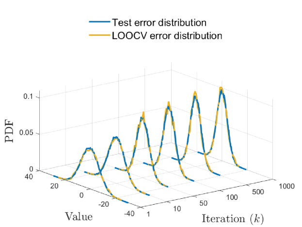
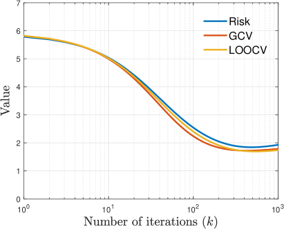
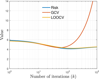
Our second result concerns LOOCV and establishes that it is consistent for the out-of-sample prediction risk, in a uniform sense over the GD path. For this, we make only weak assumptions on the feature distribution and do not assume a well-specified model (i.e., allowing the true regression function to be nonlinear). One interpretation is that this suggests that the failure of GCV lies in its ability to approximate LOOCV, and not with LOOCV itself. Figure 1 showcases an empirical illustration of our main results, which we summarize below.

1.1 Summary of main results

• GCV inconsistency. Under a proportional asymptotics model where the number of features $p$ and observations $n$ scale proportionally, and assuming a well-specified linear model and isotropic features, we show that GCV is inconsistent for estimating the prediction risk throughout basically the entire GD path (Theorem 1). We prove this result by separately deriving the asymptotic limits for the GCV estimator and the true risk of early-stopped GD, and then showing that they do not match.

• LOOCV consistency. Under a proportional asymptotics model again, we show that LOOCV is consistent for estimating the prediction risk of early-stopped GD, in a uniform sense over the GD iterations (Theorem 2). Our analysis only requires the distributions of the features and noise to satisfy a $T_{2}$-inequality, which is quite weak. In particular, we do not assume any specific model for the regression function. As a consequence of uniformity, we establish that the risk of the LOOCV-tuned iterate almost surely matches that of the oracle-tuned iterate. Furthermore, we also propose an implementation of the LOOCV with lower computational complexity compared to the naive implementation (Proposition 7).

• Functional consistency. Beyond prediction risk, we propose a natural extension of LOOCV to estimate general functionals of the prediction error distribution for early-stopped GD, which is a plug-in approach based on the empirical distribution of LOOCV errors (Theorem 3). As an application, we use this to consistently estimate the quantiles of the prediction error distribution for GD iterates, allowing the construction of prediction intervals with asymptotically correct nominal coverage conditional on the training data (Theorem 4).

1.2 Related work

GD and its variants are central tools for training modern machine learning models. These methods, especially stochastic gradient methods, can be highly scalable. But, somewhat surprisingly, overparameterized models trained with GD and variants also often generalize well, even in the absence of explicit regularizers and with noisy labels (Zhang et al., 2017). This behavior is often attributed to the fact that the GD iterates are subject to a kind of implicit regularization (Wilson et al., 2017; Gunasekar et al., 2018a, b). Implicit regularization has a rich history in machine learning and has appeared in some of the first insights into the advantages of early stopping in neural network training (Morgan and Bourlard, 1989). A parallel idea in numerical analysis is known as the Landweber iteration (Landweber, 1951; Strand, 1974). There is a rich literature on early stopping in the context of boosting (Bühlmann and Yu, 2003; Rosset et al., 2004; Zhang and Yu, 2005; Yao et al., 2007; Bauer et al., 2007; Raskutti et al., 2014; Wei et al., 2017). Furthermore, several precise correspondences between GD and ridge penalized estimators have been established by Suggala et al. (2018); Neu and Rosasco (2018); Ali et al. (2019, 2020), among others.

CV is a standard approach in statistics for parameter tuning and model selection. For classic work on CV, see, e.g., Allen (1974); Stone (1974, 1977); Geisser (1975). For practical surveys, see Arlot and Celisse (2010); Zhang and Yang (2015). More recently, there has been renewed interest in developing a modern theory for CV, with contributions from Kale et al. (2011); Kumar et al. (2013); Celisse and Guedj (2016); Austern and Zhou (2020); Bayle et al. (2020); Lei (2020); Rad et al. (2020), among others. As LOOCV is, in general, computationally expensive, there has also been recent work in designing and analyzing approximate leave-one-out methods to address the computational burden; see, e.g., Wang et al. (2018); Stephenson and Broderick (2020); Wilson et al. (2020); Rad and Maleki (2020); Auddy et al. (2023).

GCV is an approximation to LOOCV and is closely connected to what is called the “shortcut” leave-one-out formula for linear smoothers. The classic work on GCV includes Craven and Wahba (1979); Golub et al. (1979); Li (1985, 1986, 1987). Recently, GCV has garnered significant interest, as it has been found to be consistent for out-of-sample prediction risk in various high-dimensional settings; see, e.g., Hastie et al. (2022); Adlam and Pennington (2020); Patil et al. (2021, 2022b); Wei et al. (2022); Du et al. (2023); Han and Xu (2023); Patil and LeJeune (2024). While originally defined for linear smoothers, the idea of using similar degrees-of-freedom adjustments can be extended beyond this original scope to nonlinear predictors; see, e.g., Bayati and Montanari (2011); Bayati et al. (2013); Miolane and Montanari (2021); Bellec and Shen (2022); Bellec (2023).

Most of the aforementioned papers on CV have focused on estimators that are defined as solutions to empirical risk minimization problems. There has been little work that studies CV for iterates of optimization algorithms like GD, which are commonly used to find solutions (train models) in practice. Very recently, Luo et al. (2023) consider approximating LOOCV for iterative algorithms. They propose an algorithm that is more efficient than the naive LOOCV when $p\ll n$. They also show that their method approximates LOOCV well. In our work, we instead focus on analyzing LOOCV itself, along with GCV, for least squares problems, which we view as complementary to their work. Moreover, our analysis is in the proportional asymptotic regime, where $p\asymp n$.

2 Preliminaries

In this section, we define the main object of study: early-stopped GD applied to the least squares loss. We then precisely define the risk metric of interest and describe the risk estimators based on LOOCV and GCV.

2.1 Early-stopped gradient descent

Consider a standard regression setting, where we observe independent and identically distributed samples $\{(x_{i},y_{i})\}\in\mathbb{R}^{p+1}\times\mathbb{R}$ for $i\in[n]$. Here, each $x_{i}\in\mathbb{R}^{p+1}$ denotes a feature vector and $y_{i}\in\mathbb{R}$ its response value. The last entry of each $x_{i}$ is set to $1$ to accommodate an intercept term in the regression model. Let $X\in\mathbb{R}^{n\times(p+1)}$ denote the feature matrix whose $i$-th row contains $x_{i}^{\top}$, and $y\in\mathbb{R}^{n}$ the response vector whose $i$-th entry contains $y_{i}$.

We focus on the ordinary least squares problem:

$$\addcontentsline{lla}{section}{\numberline{\string\crtrefnumber{eq:ols-obj}}{e}q:ols-obj}\mathop{\mathrm{minimize}}_{\beta\in\mathbb{R}^{p+1}}\;\frac{1}{2n}\|y-X\beta\|_{2}^{2},$$ (1)

and we study the sequence of estimates defined by applying gradient descent (GD) to the squared loss in (1). Specifically, given step sizes $\delta=(\delta_{0},\dots,\delta_{K-1})\in\mathbb{R}^{K}$, and initializing GD at the origin, $\widehat{\beta}_{0}=0$, the GD iterates are defined recursively as follows:

$$\addcontentsline{lla}{section}{\numberline{\string\crtrefnumber{eq:gd-iterate}}{e}q:gd-iterate}\widehat{\beta}_{k}=\widehat{\beta}_{k-1}+\frac{\delta_{k-1}}{n}X^{\top}(y-X\widehat{\beta}_{k-1}),\quad k\in[K].$$ (2)

Let $(x_{0},y_{0})\in\mathbb{R}^{p+1}\times\mathbb{R}$ denote a test point drawn independently from the same distribution as the training data. We are interested in estimating the out-of-sample prediction risk along the GD path. More precisely, we are interested in estimating the squared prediction error $R(\widehat{\beta}_{k})$ achieved by the GD iterate at each step $k\in[K]$, defined as:

$$\addcontentsline{lla}{section}{\numberline{\string\crtrefnumber{eq:pred-risk}}{e}q:pred-risk}R(\widehat{\beta}_{k})=\mathbb{E}_{x_{0},y_{0}}\big{[}(y_{0}-x_{0}^{\top}\widehat{\beta}_{k})^{2}\mid X,y\big{]}.$$ (3)

Note that our notion of risk here is conditional on the training features and responses, $X,y$.

2.2 GCV and LOOCV

Next, we present an overview of the LOOCV and GCV estimators associated with GD iterates. First, we describe the estimators that correspond to the squared prediction risk. The exact LOOCV estimator for the squared prediction risk of $\widehat{\beta}_{k}$ is defined as:

$$\addcontentsline{lla}{section}{\numberline{\string\crtrefnumber{eq:loocv-risk}}{e}q:loocv-risk}\widehat{R}^{\mathrm{loo}}(\widehat{\beta}_{k})=\frac{1}{n}\sum_{i=1}^{n}(y_{i}-x_{i}^{\top}\widehat{\beta}_{k,-i})^{2},$$ (4)

where $\widehat{\beta}_{k,-i}$ denotes the GD iterate after $k$ iterations trained on the data $X_{-i},y_{-i}$, which excludes the $i$-th sample from the full data $X,y$. To be explicit, $X_{-i}$ is the result of removing the $i$-th row of $X$, and $y_{-i}$ is the result of removing the $i$-th coordinate of $y$.

Towards defining GCV, suppose that we have a predictor $\widehat{f}\colon\mathbb{R}^{p+1}\to\mathbb{R}$ which is a linear smoother, i.e., $\widehat{f}(\mathbf{x})=\mathbf{s}_{\mathbf{x}}^{\top}\mathbf{y}$ for some vector $\mathbf{s}_{\mathbf{x}}\in\mathbb{R}^{n}$ which depends only on the feature matrix $\mathbf{X}$ and the test point $\mathbf{x}$. The smoothing matrix associated with the predictor $\widehat{f}$ is denoted $\mathbf{S}\in\mathbb{R}^{n\times n}$ and defined to have rows $\mathbf{s}_{\mathbf{x}_{1}}^{\top},\dots,\mathbf{s}_{\mathbf{x}_{n}}^{\top}$. The GCV estimator of the prediction risk of $\widehat{f}$ is defined as:

$$\widehat{R}^{\mathrm{gcv}}(\widehat{f})=\frac{\|\mathbf{y}-\mathbf{S}\mathbf{y}\|_{2}^{2}/n}{(1-\operatorname{tr}[\mathbf{S}]/n)^{2}}.$$

The numerator here is the training error, which is of course typically biased downward, meaning that it typically underestimates the prediction error. The denominator corrects for this downward bias, often referred to as the “optimism” of the training error, with $1-\operatorname{tr}[\mathbf{S}]/n$ acting as a degrees-of-freedom correction, which is smaller the more complex the model (the larger the trace of $\mathbf{S}$).

A short calculation shows that each GD iterate can be represented as a linear smoother, i.e., the in-sample predictions can be written as $X\widehat{\beta}_{k}=H_{k}y$, where

$$H_{k}=\sum_{j=0}^{k-1}\frac{\delta_{j}}{n}X\prod_{r=1}^{k-j-1}\big{(}{I}_{p+1}-\delta_{k-r}\widehat{\Sigma}\big{)}X^{\top},$$

and we denote by $\widehat{\Sigma}=X^{\top}X/n$ the sample covariance matrix. This motivates us to estimate its prediction risk using GCV:

$$\addcontentsline{lla}{section}{\numberline{\string\crtrefnumber{eq:gcv-risk}}{e}q:gcv-risk}\widehat{R}^{\mathrm{gcv}}(\widehat{\beta}_{k})=\frac{1}{n}\sum_{i=1}^{n}\frac{(y_{i}-x_{i}^{\top}\widehat{\beta}_{k})^{2}}{(1-\operatorname{tr}[H_{k}]/n)^{2}}.$$ (5)

Perhaps surprisingly, as we will see shortly in Section 3, GCV does not consistently estimate the prediction risk for GD iterates, even if we assume a well-specified linear model. On the other hand, we will show in Section 4 that LOOCV is uniformly consistent along the GD path. We also later propose a modified “shortcut” in Section 5 that (1) exactly tracks the LOOCV estimates, and (2) is computationally more efficient than the naive implementation of LOOCV.

3 GCV inconsistency

In this section, we prove that GCV is generically inconsistent for estimating the squared prediction risk, even under a well-specified linear model with isotropic Gaussian features. For simplicity, in this section only, we consider fixed step sizes $\delta_{k}=\delta$ and omit the intercept term. We impose the following assumptions on the feature and response distributions.

Assumption A (Feature distribution).

Each feature vector $x_{i}\in\mathbb{R}^{p}$, for $i\in[n]$, contains i.i.d. Gaussian entries with mean $0$ and variance $1$.

Assumption B (Response distribution).

Each response variable $y_{i}$, for $i\in[n]$, follows a well-specified linear model: $y_{i}=x_{i}^{\top}\beta_{0}+\varepsilon_{i}$. Here, $\beta_{0}\in\mathbb{R}^{p}$ is an unknown signal vector satisfying $\lim_{p\to\infty}\|\beta_{0}\|_{2}^{2}=r^{2}<\infty$, and $\varepsilon_{i}$ is a noise variable, independent of $x_{i}$, drawn from a Gaussian distribution with mean $0$ and variance $\sigma^{2}<\infty$.

The zero-mean condition for each $y_{i}$ is used only for simplicity. (Accordingly, we do not include an additional intercept term in the model, implying that $x_{i}\in\mathbb{R}^{p}$.) Although one could establish the inconsistency of GCV under more relaxed assumptions, we choose to work under Assumptions A and B to highlight that GCV fails even under favorable conditions.

We analyze the behavior of the estimator in the proportional asymptotics regime, where both the number of samples $n$ and the number of features $p$ tend to infinity, and their ratio $p/n$ converges to a constant $\zeta_{\ast}\in(0,\infty)$. This regime has received considerable attention recently in high-dimensional statistics and machine learning theory.

The dynamics of GD are determined by both the step size $\delta$ and the iterate number $k$. We study a regime in which $\delta\to 0$ and $k\to\infty$ as $n,p\to\infty$, which effectively reduces the GD iterates to a continuous-time gradient flow, as studied in other work (Ali et al., 2019; Celentano et al., 2021; Berthier et al., 2023). Our main negative result, on GCV, is given next.

Theorem 1 (Inconsistency of GCV).

Suppose that $(x_{i},y_{i})$, $i\in[n]$ are i.i.d., and satisfy both Assumptions A and B, where either $r^{2}>0$ or $\sigma^{2}>0$. As $n,p\to\infty$, assume $p/n\to\zeta_{\ast}$, and $k\to\infty$, $\delta\to 0$ such that $k\delta\to T$, where $T,\zeta_{\ast}>0$ are constants. Then, for every fixed $\zeta_{\ast}>0$, it holds that for almost all $T>0$ (i.e., all $T>0$ except for a set of Lebesgue measure zero),

$$\addcontentsline{lla}{section}{\numberline{\string\crtrefnumber{eq:gcv_inconsistency}}{e}q:gcv_{i}nconsistency}\Big{|}\widehat{R}^{\mathrm{gcv}}(\widehat{\beta}_{k})-R(\widehat{\beta}_{k})\Big{|}\not\xrightarrow{\mathrm{p}}0,$$ (6)

where we recall that $\widehat{R}^{\mathrm{gcv}}(\widehat{\beta}_{k})$ and $R(\widehat{\beta}_{k})$ are as defined in (5) and (3), respectively.

In other words, the theorem says that GCV does not consistently track the true prediction risk at basically any point along the GD path (in the sense that GCV can only possibly be consistent at a Lebesgue measure zero set of times $T$). It is worth noting that the inconsistency here can be severe especially in the overparameterized regime, when $\zeta_{\ast}>1$. In particular, in this regime, it is easy to show that if $k\delta\to\infty$ (rather than $k\delta\to T$ for a finite limit $T$), then $\lim_{k\to\infty}\widehat{R}^{\mathrm{gcv}}(\widehat{\beta}_{k})\to\infty$, while $R(\widehat{\beta}_{K})\to r^{2}+\sigma^{2}$, under the assumptions of Theorem 1. This is evident in Figure 1.

4 LOOCV consistency

Despite the inconsistency of GCV, LOOCV remains consistent for GD. This section establishes a uniform consistency result for LOOCV along the GD path.

4.1 Squared risk

We begin by focusing on squared prediction risk. The technical crux of our analysis revolves around establishing certain concentration properties of the LOOCV estimator $\widehat{R}^{\mathrm{loo}}(\widehat{\beta}_{k})$, and to do so, we leverage Talagrand’s $T_{2}$-inequality (Gozlan, 2009). Specifically, under the assumption that both the entries of the feature and noise distributions satisfy the $T_{2}$-inequality, we show that $\widehat{R}^{\mathrm{loo}}(\widehat{\beta}_{k})$ behaves approximately as a Lipschitz function of these random variables. Together, these results enable us to leverage powerful dimension-free concentration inequalities.

The inspiration for using $T_{2}$-inequality comes from the recent work of Avelin and Viitasaari (2022). They assume that the data distribution satisfies the logarithmic Sobolev inequality (LSI), which is a strictly stronger condition than what we assume here. Furthermore, they only consider fixed $p$ and do not consider iterative algorithms. The extensions we pursue present considerable technical challenges and require us to delicately upper bound the norms of various gradients involved. Below we give a formal definition of what it means for a distribution to satisfy the $T_{2}$-inequality.

Definition 1 ($T_{2}$-inequality).

We say a distribution $\mu$ satisfies the $T_{2}$-inequality if there exists a constant $\sigma(\mu)\geq 0$, such that for every distribution $\nu$,

$$\addcontentsline{lla}{section}{\numberline{\string\crtrefnumber{eq:T2-inequality}}{e}q:T2-inequality}W_{2}(\mu,\nu)\leq\sqrt{2\sigma^{2}(\mu)D_{\mathrm{\texttt{KL}}}\big{(}\nu\big{\|}\mu\big{)}},$$ (7)

where $W_{2}(\cdot,\cdot)$ is the 2-Wasserstein distance, and $D_{\mathrm{\texttt{KL}}}(\cdot\|\cdot)$ the Kullback-Leibler divergence.

The $T_{2}$-inequality is, in some sense, a necessary and sufficient condition for dimension-free concentration. We refer interested readers to Theorem 4.31 in Van Handel (2014) for more details (see also Section S.5.2 for further facts related to the $T_{2}$-inequality).

One prominent example of distributions that satisfy the $T_{2}$-inequality are distributions that satisfy the log Sobolev inequality (LSI); Section S.5.1 gives more details. We note that all distributions that are strongly log-concave satisfy the LSI, as do many non-log-concave distributions, such as Gaussian convolutions of distributions with bounded support (Chen et al., 2021). Next, we formally state our assumptions for this section, starting with the feature distribution.

Assumption C (Feature distribution).

1. Each feature vector $x_{i}\in\mathbb{R}^{p+1}$, for $i\in[n]$, decomposes as $x_{i}^{\top}=((\Sigma^{1/2}z_{i})^{\top},1)$, where $z_{i}\in\mathbb{R}^{p}$ has i.i.d. entries $z_{ij}$ drawn from $\mu_{z}$.

2. The distribution $\mu_{z}$ has mean $0$, variance $1$, and satisfies the $T_{2}$-inequality with constant $\sigma_{z}$.

3. There covariance matrix satisfies $\|\Sigma\|_{\operatorname{op}}\leq\sigma_{\Sigma}$ for a constant $\sigma_{\Sigma}$.

To be clear, in the above $\sigma_{z},\sigma_{\Sigma}$ are constants that are not allowed to change with $n,p$. It is worth emphasizing that we do not require the smallest eigenvalue of $\Sigma$ in Assumption C to be bounded away from $0$. This is possible because the iterates along the GD path are implicitly regularized. This is similar to not requiring a lower bound on the smallest eigenvalue for ridge regression when $\lambda>0$ (as opposed to ridgeless regression, where we do need such an assumption); see Dobriban and Wager (2018); Patil et al. (2021). We also impose the following assumptions on the response distribution.

Assumption D (Response distribution).

1. Each $y_{i}=f(x_{i})+\varepsilon_{i}$, for $i\in[n]$,  where $\varepsilon_{i}$ is independent of $x_{i}$ and drawn from $\mu_{\varepsilon}$.

2. The distribution $\mu_{\varepsilon}$ has mean $0$ and satisfies the $T_{2}$-inequality with constant $\sigma_{\varepsilon}$.

3. The regression function $f$ is $L_{f}$-Lipschitz continuous, where without loss of generality, $L_{f}\leq 1$.

4. Finally, $\mathbb{E}[y_{i}^{8}]\leq m_{8}$, $\mathbb{E}[y_{i}^{4}]\leq m_{4}$, and $\mathbb{E}[y_{i}^{2}]\leq m_{2}$.

In the above $\sigma_{\varepsilon},m_{2},m_{4},m_{8}$ are constants that are not allowed to change with $n,p$. We note that the assumptions we impose in this section are strictly weaker than those in Section 3. In particular, it is notable that we do not require $\mathbb{E}[y_{i}\,|\,x_{i}=x]$ to be linear in $x$. We are ready to give our first main positive result, on LOOCV for squared risk.

Theorem 2 (Squared risk consistency of LOOCV).

Suppose that $(x_{i},y_{i})$, $i\in[n]$ are i.i.d., and satisfy both Assumptions C and D. In addition, assume that there are constants $\Delta,B_{0},\zeta_{L},\zeta_{U}$ (independent of $n,p$) such that: (1) $\sum_{k=1}^{K}\delta_{k-1}\leq\Delta$, (2) $\|\widehat{\beta}_{0}\|_{2}\leq B_{0}$, and (3) $0<\zeta_{L}\leq p/n\leq\zeta_{U}<\infty$. Furthermore, let $K=o(n\cdot(\log n)^{-3/2})$. Then, as $n,p\to\infty$,

$$\addcontentsline{lla}{section}{\numberline{\string\crtrefnumber{eq:loocv-consistency-squared}}{e}q:loocv-consistency-squared}\max_{k\in[K]}\,\Big{|}\widehat{R}^{\mathrm{loo}}(\widehat{\beta}_{k})-R(\widehat{\beta}_{k})\Big{|}\xrightarrow{\mathrm{a.s.}}0,$$ (8)

where we recall that $\widehat{R}^{\mathrm{loo}}(\widehat{\beta}_{k})$ and $R(\widehat{\beta}_{k})$ are as defined in (4) and (3), respectively.

The convergence guarantee in Theorem 2 is strong in the sense that it is uniform across the entire GD path, and convergence occurs conditional on the training data. Uniformity in particular allows us to argue that tuning based on LOOCV guarantees asymptotically optimal risk. We cover this next, where we also generalize our study from squared error to general error functionals.

4.2 General risk functionals

We now extend our theory from the last subsection to cover general risk functionals, subject to only mild regularity conditions. Let $\psi\colon\mathbb{R}^{2}\to\mathbb{R}$ be an error function, which takes as input the predictand (first argument) and prediction (second argument). We define a corresponding risk functional as:

$$\addcontentsline{lla}{section}{\numberline{\string\crtrefnumber{eq:pred-functional}}{e}q:pred-functional}\Psi(\widehat{\beta}_{k})=\mathbb{E}_{x_{0},y_{0}}\big{[}\psi(y_{0},x_{0}^{\top}\widehat{\beta}_{k})\mid X,y\big{]}.$$ (9)

One can naturally define an estimator for $\Psi(\widehat{\beta}_{k})$ based on LOOCV using the “plug-in” principle:

$$\addcontentsline{lla}{section}{\numberline{\string\crtrefnumber{eq:Tloocv}}{e}q:Tloocv}{\widehat{\Psi}}^{\mathrm{loo}}(\widehat{\beta}_{k})=\frac{1}{n}\sum_{i=1}^{n}\psi(y_{i},x_{i}^{\top}\widehat{\beta}_{k,-i}).$$ (10)

Our second main positive result shows that this LOOCV plug-in estimator is uniformly consistent along the GD path.

Theorem 3 (Functional consistency of LOOCV).

Under the conditions of Theorem 2, suppose that $\psi:\mathbb{R}^{2}\to\mathbb{R}$ is differentiable and satisfies $\|\nabla\psi(u)\|_{2}\leq C_{\psi}\|u\|_{2}+\bar{C}_{\psi}$ for all $u\in\mathbb{R}^{2}$ and for constants $C_{\psi},\bar{C}_{\psi}\geq 0$. Then, as $n,p\to\infty$,

$$\addcontentsline{lla}{section}{\numberline{\string\crtrefnumber{eq:loocv-consistency-functional}}{e}q:loocv-consistency-functional}\max_{k\in[K]}\,\big{|}\widehat{\Psi}^{\mathrm{loo}}(\widehat{\beta}_{k})-\Psi(\widehat{\beta}_{k})\big{|}\xrightarrow{\mathrm{a.s.}}0.$$ (11)

where we recall that $\widehat{R}^{\mathrm{loo}}(\widehat{\beta}_{k})$ and $R(\widehat{\beta}_{k})$ are as defined in (10) and (9), respectively.

As consequence of (11), LOOCV can be used to tune early stopping. Specifically, if we define $k_{\ast}=\mathop{\mathrm{arg\,min}}_{k\in[K]}\widehat{\Psi}^{\mathrm{loo}}(\widehat{\beta}_{k})$, then as $n,p\to\infty$,

$$\addcontentsline{lla}{section}{\numberline{\string\crtrefnumber{eq:loocv-consistency-functional-tuned}}{e}q:loocv-consistency-functional-tuned}\big{|}\Psi(\widehat{\beta}_{k_{\ast}})-\min_{k\in[K]}\Psi(\widehat{\beta}_{k})\big{|}\xrightarrow{\mathrm{a.s.}}0.$$ (12)

Thanks to Theorem 3, we can consistently estimate the quantiles of the prediction error distribution using the empirical quantiles of the distribution that puts $1/n$ mass at each LOOCV residual.

Theorem 4 (Coverage guarantee).

Under the conditions of Theorem 3, assume further that the distribution of the noise $\varepsilon_{i}$ is continuous with density bounded by $\kappa_{\mathsf{pdf}}$. Denote by $\widehat{\alpha}_{k}(q)$ the $q$-quantile of $\{y_{i}-x_{i}^{\top}\widehat{\beta}_{k,-i}:i\in[n]\}$. Then, for any quantile levels $0\leq q_{1}\leq q_{2}\leq 1$, letting $\mathcal{I}_{k}=[\widehat{\alpha}_{k}(q_{1}),\widehat{\alpha}_{k}(q_{2})]$, we have as $n,p\to\infty$,

$$\addcontentsline{lla}{section}{\numberline{\string\crtrefnumber{eq:loocv-coverage}}{e}q:loocv-coverage}\max_{k\in[K]}\,\mathbb{P}_{(x_{0},y_{0})}\big{(}y_{0}-x_{0}^{\top}\widehat{\beta}_{k}\in\mathcal{I}_{k}\mid X,y\big{)}\xrightarrow{\mathrm{a.s.}}q_{2}-q_{1}.$$ (13)

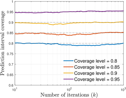
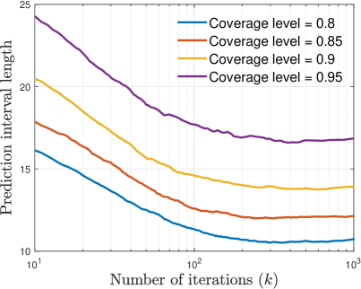
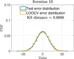
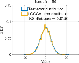
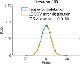
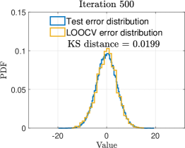
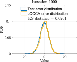
Note that Theorem 4 provides conditional rather than marginal coverage guarantees for the specific data $X,y$ that we observe. Figure 3 provides an example. Finally, we remark that the empirical distribution of the LOOCV errors can be shown to weakly converge to the true error distribution, almost surely. This is illustrated in Figure 3, with Figure S.22 providing an additional visualization.

Figure 2: LOOCV provides (asymptotically) valid prediction intervals, for various nominal coverage levels. We investigate the empirical coverage and length of LOOCV prediction intervals along the GD path, at varying coverage levels. We consider an overparameterized regime with $n=2500$ and $p=5000$. The features are drawn from a Gaussian distribution with a covariance structure: $\Sigma_{ij}=\rho^{|i-j|}$ for all $i,j$ and $\rho=0.25$. The response is generated from a nonlinear model with heavy-tailed noise: $t$-distribution with 5 degrees of freedom. The linear component of $\mathbb{E}[y_{i}\,|\,x_{i}=x]$ is aligned with the top eigenvector of $\Sigma$. GD is run with a constant step size of $0.01$. (See Appendix S.11 for further details on the experimental setup.) We can see that the prediction intervals generally have excellent finite-sample coverage along the entire path (left), and the smallest prediction length is typically obtained at a large iteration of GD (right).

Figure 3: Empirical distribution of LOOCV errors tracks the true test error distribution along the entire GD trajectory. We consider the same setup as in Figure 3 with an overparameterized regime of $n=2500$ and $p=5000$. (See Appendix S.11 for further details on the experimental setup.) The blue curve in each panel represents a histogram of true prediction error errors (computed via Monte Carlo), while the yellow curve represents a histogram of the LOOCV errors. Each panel represents a given GD iteration, and we see strong agreement in the histograms throughout. Furthermore, due to the structure of the simulation setup, the test error distribution begins to exhibit lower variance as the iterations proceed.

5 Discussion

In the paper, we establish a significant discrepancy between LOOCV and GCV when it comes to estimating the prediction risk of early-stopped GD for least squares regression in high dimensions. While LOOCV is consistent in a strong uniform sense, GCV fails along essentially the entire path. This is especially curious considering that both LOOCV and GCV are uniformly consistent for the risk of explicitly regularized estimators such as ridge regression (Patil et al., 2021, 2022b). Therefore, this discrepancy also highlights a difference between GD and ridge regression, which is interesting in light of all of the existing work that establishes similarities between the two (Suggala et al., 2018; Neu and Rosasco, 2018; Ali et al., 2019).

Recall that GCV is generally tied to the “shortcut” formula for the leave-one-out (LOO) predictions in linear smoothers, where we adjust the training error for the $i$-th sample by $1-\operatorname{tr}[S]/n$ (GCV), in place of $1-S_{ii}/n$ (shortcut formula). A key part of the failure of GCV for GD is that its LOO predictions behave differently than those in ridge regression, as we discuss in what follows.

5.1 LOO predictions in ridge regression versus gradient descent

For ridge regression, the LOO predictions, and hence LOOCV residuals, can be computed directly from the residuals of the full model (the model fit on the full data $X,y$) using a shortcut formula (Golub et al., 1979; Hastie, 2020). This is computationally important since it means we can compute LOOCV without any refitting.

An elegant way to verify this shortcut formula involves creating an augmented system that allows us to identify the LOO prediction, which we briefly describe here. (We omit the intercept in the model, for simplicity.) For a given data point $(x_{i},y_{i})$ that is to be left out, we seek to solve the problem:

$$\addcontentsline{lla}{section}{\numberline{\string\crtrefnumber{eq:ridge-loo}}{e}q:ridge-loo}\mathop{\mathrm{minimize}}_{\beta\in\mathbb{R}^{p}}\;\|y_{-i}-X_{-i}\beta\|_{2}^{2}+\lambda\|\beta\|_{2}^{2}.$$ (14)

Denoting its solution by $\widehat{\beta}_{\lambda,-i}$, the corresponding LOO prediction is therefore $x_{i}^{\top}\widehat{\beta}_{\lambda,-i}$. Let us now imagine that we “augment” the data $X_{-i},y_{-i}$ set by adding the pair $(x_{i},x_{i}^{\top}\widehat{\beta}_{\lambda,-i})$ in place of the $i$-th sample. Denote by $\widetilde{y}_{-i}\in\mathbb{R}^{n}$ the response vector in the augmented data set, and $X$ the feature matrix (it is unchanged from the original data set). Denote by $\widetilde{\beta}_{\lambda,-i}$ the ridge estimator fit on the augmented data set $X,\widetilde{y}_{-i}$, which solves:

$$\addcontentsline{lla}{section}{\numberline{\string\crtrefnumber{eq:ridge-augmented}}{e}q:ridge-augmented}\mathop{\mathrm{minimize}}_{\beta\in\mathbb{R}^{p}}\;\|\widetilde{y}_{-i}-X\beta\|_{2}^{2}+\lambda\|\beta\|_{2}^{2}.$$ (15)

Problems (14) and (15) admit the same solution, because in the latter we have only added a single sample $x_{i}^{\top}\widehat{\beta}_{\lambda,-i}$ and this attains zero loss at the solution in the former. Thus, we have $\widetilde{\beta}_{\lambda,-i}=\widehat{\beta}_{\lambda,-i}$, and we can write the predicted value for the $i$-th observation as follows:

$$x_{i}^{\top}\widehat{\beta}_{\lambda,-i}=\sum_{j\neq i}[H_{\lambda}]_{ij}y_{j}+[H_{\lambda}]_{ii}(x_{i}^{\top}\widehat{\beta}_{\lambda,-i}),$$

where $H_{\lambda}\in\mathbb{R}^{n\times n}$ is the ridge smoothing matrix associated with full feature matrix $X$ at regularization level $\lambda$. Rearranging, we have:

$$x_{i}^{\top}\widehat{\beta}_{\lambda,-i}=\frac{\sum_{j\neq i}[H_{\lambda}]_{ij}y_{j}}{1-[H_{\lambda}]_{ii}},$$

or equivalently, in terms of residuals:

$$\addcontentsline{lla}{section}{\numberline{\string\crtrefnumber{eq:ridge-loo-shortcut}}{e}q:ridge-loo-shortcut}y_{i}-x_{i}^{\top}\widehat{\beta}_{\lambda,-i}=\frac{y_{i}-\sum_{j}[H_{\lambda}]_{ij}y_{j}}{1-[H_{\lambda}]_{ii}}=\frac{y_{i}-x_{i}^{\top}\widehat{\beta}_{\lambda}}{1-[H_{\lambda}]_{ii}}.$$ (16)

Meanwhile, for the GD path, the analogous construction does not reproduce the LOO predictions. More precisely, let $\widehat{\beta}_{k,-i}$ be the GD iterate at step $k$, run on the LOO data set $X_{-i},y_{-i}$. As before, imagine that we augment this data set with the pair $(x_{i},x_{i}^{\top}\widehat{\beta}_{k,-i})$. Denote again by $X$ the feature matrix and $\widetilde{y}_{-i}\in\mathbb{R}^{n}$ the response vector in the augmented data set, and denote by $\widetilde{\beta}_{k,-i}$ the result of running $k$ iterations of GD on $X,\widetilde{y}_{-i}$. In general, we will have $\widehat{\beta}_{k,-i}\neq\widetilde{\beta}_{k,-i}$.

Figure 4: Illustrations of the differences between the LOO systems for ridge regression (left) and GD (right).

The underlying reason for this is that, even though the GD iterates can be written as a solution to a regularized least squares problem, the regularizer in this problem depends on the data (which is not true in ridge). For constant step sizes all equal to $\delta$, the GD iterate (2) can be shown to solve:

$$\mathop{\mathrm{minimize}}_{\beta\in\mathbb{R}^{p}}\;\|y-X\beta\|_{2}^{2}/2n+\beta^{\top}Q_{k}\beta,$$

where $Q_{k}=X^{\top}X/n((I_{p}-\delta X^{\top}X/n)^{k}-I_{p})^{-1}$. The regularization term is not only a function of $\delta$ and $k$, but also of $X$. This complicates the LOO predictions.

5.2 Modified augmented system for LOO in GD

Identifying this failure of GD, as summarized in Figure 4, also helps us modify the augmentation trick so that we can recover the LOO predictions. Precisely, for $k\in[K]$ and $i,j\in[n]$, let

$$(\widetilde{y}_{k,-i})_{j}=\begin{cases}y_{j},&j\neq i\vspace{0.2cm}\\ x_{i}^{\top}\widehat{\beta}_{k,-i},&j=i.\end{cases}$$

Define the vector $\widetilde{y}_{k,-i}=(\widetilde{y}_{k,-i})_{j\leq n}$, and let $\widetilde{\beta}_{k,-i}$ be the iterate obtained by running GD for $k$ steps where at each step $\ell\leq k$, the augmented response vector $\widetilde{y}_{\ell,-i}$ is used in the gradient update. See Figure 5 for an illustration. Next, we show that this scheme recovers the LOO coefficients along the GD path.

Proposition 5 (Correctness of the modified augmented system).

For all $k\in[K]$ and $i\in[n]$, it holds that $\widetilde{\beta}_{k,-i}=\widehat{\beta}_{k,-i}$.

In other words, to recreate LOO coefficients from $k$-step GD, we must use an augmented response vector not only at step $k$ but at every iteration before $k$ as well. With this insight, we can represent the LOO predictions in a certain linear smoother form.

Proposition 6 (Smoother representation for the modified augmented system).

For all $k\in[K]$ and $i\in[n]$, there is a vector $(h_{ij}^{(k)})_{j\leq n}$ and scalar $b_{i}^{(k)}$ depending $\delta=(\delta_{0},\dots\delta_{k-1})$ and $X$ such that:

$$x_{i}^{\top}\widehat{\beta}_{k,-i}=x_{i}^{\top}\widetilde{\beta}_{k,-i}=\sum_{j=1}^{n}h_{ij}^{(k)}y_{j}+b_{i}^{(k)}.$$

Figure 5: Illustration of the modified augmented system for LOO in GD.

5.3 Towards exact and efficient LOOCV for GD?

We can unravel the relationships in LOO coefficients between iterations of the modified augmented system to arrive at explicit recursive forms for $(h_{ij}^{(k)})_{j\leq n}$ and $b_{i}^{(k)}$ in Proposition 6, given next.

Proposition 7 (Recursive shortcut formula for LOO predictions in GD).

For all $k\in[K]$ and $i\in[n]$,

$$x_{i}^{\top}\widehat{\beta}_{k,-i}=x_{i}^{\top}\widehat{\beta}_{k}+A_{i,k}\|x_{i}\|_{2}^{2}+\sum_{j=1}^{k-1}B_{i,k}^{(j)}x_{i}^{\top}(X^{\top}X)^{j}x_{i},$$

where

$$A_{i,k+1} =A_{i,k}+\frac{2\delta_{k}A_{i,k}\|x_{i}\|_{2}^{2}}{n}+\sum_{j=1}^{k-1}\frac{2\delta_{k}B_{i,k}^{(j)}x_{i}^{\top}(X^{\top}X)^{j}x_{i}}{n}+\frac{2\delta_{k+1}(x_{i}^{\top}\widehat{\beta}_{k}-y_{i})}{n},$$

$$B_{i,k+1}^{(1)} =B_{i,k}^{(1)}-\frac{2\delta_{k}A_{i,k}}{n},$$

$$B_{i,k+1}^{(j)} =B_{i,k}^{(j)}-\frac{2\delta_{k}B_{i,k}^{(j-1)}}{n},\quad 2\leq j\leq k,$$

and we make the convention that $B_{i,k}^{(k)}=0$.

Using this proposition, we can estimate generic prediction risk functionals as follows. Abbreviating $\mathcal{H}_{ij}=x_{i}^{\top}(X^{\top}X)^{j}x_{i}$, to estimate the risk functional (9), we use:

$$\addcontentsline{lla}{section}{\numberline{\string\crtrefnumber{eq:Tloocv-shortcut}}{e}q:Tloocv-shortcut}\Psi^{\mathrm{loo}}(\widehat{\beta}_{k})=\frac{1}{n}\sum_{i=1}^{n}\psi\bigg{(}y_{i},\,x_{i}^{\top}\widehat{\beta}_{k}+A_{i,k}\|x_{i}\|_{2}^{2}+\sum_{j=1}^{k-1}B_{i,k}^{(j)}\mathcal{H}_{ij}\bigg{)}.$$ (17)

To be clear, (17) is an exact shortcut formula for (10).

In the $p\asymp n$ regime, the computational cost of a naive implementation of LOOCV for $k$-step GD is $O(n^{3}k)$. (Each GD step costs $O(n^{2})$, as we must compute $p$ inner products, each of length $n$; then multiply this by $k$ steps and $n$ LOO predictions). In comparison, the shortcut formula given above can be shown to require $O(n^{3}+n^{2}k+nk^{2})$ operations using a spectral decomposition of $X$. If $k$ is large, say, itself proportional to $n$, then we can see that the shortcut formula is more efficient.

This is certainly not meant to be the final word on efficient LOOCV along the GD path. For one, a spectral decomposition is prohibitive for large problems (more expensive than solving the original least squares problem (1)), and there may be alternative perspectives on the shortcut formula given in Proposition 7 that lead to faster implementation. Further, if $n$ is large enough, then stochastic variants of GD would be preferred in place of batch GD. All that said, the above analysis should be seen as a demonstration that exact shortcuts for LOO predictions in GD are possible, and may inspire others to develop more practical exact or approximate LOO methods.

This document serves as a supplement to the paper “Failures and Successes of Cross-Validation for Early-Stopped Gradient Descent.” The structure of the supplement is outlined below, followed by a summary of the notation and conventions used in both the main paper and this supplement. The section and figure numbers in this supplement begin with the letter “S” and the equation numbers begin with the letter “E” to differentiate them from those appearing in the main paper.

Organization

• Appendix S.1 provides the main steps involved in the proofs of Theorem 1.

  Section	Content	Purpose
  Section S.1.1	Lemmas 8 and 9	Equivalences between gradient descent and flow for risk and GCV
  Section S.1.2	Lemmas 10 and 11	Asymptotics of risk and GCV for gradient flow
  Section S.1.3	Lemma 12	Mismatch of risk and GCV asymptotics for gradient flow

• Appendix S.2 contains supporting lemmas that are used in the proof of Theorem 1.

  Section	Content	Purpose
  Section S.2.1	Lemma 13	Closeness between gradient descent and flow
  Section S.2.2	Lemmas 14 and 15	Statements of concentration results for linear and quadratic forms

• Appendix S.3 contains the proof of Theorem 1.

  Section	Content	Purpose
  Section S.3.1		Proof schematic
  Section S.3.2		Proof of Lemma 8
  Section S.3.3		Proof of Lemma 9
  Section S.3.4		Proof of Lemma 10
  Section S.3.5		Proof of Lemma 11
  Section S.3.6		Proof of Lemma 12
  Section S.3.7		A helper lemma related to the Marchenko-Pastur law

• Appendix S.4 provides the main steps involved in the proofs of Theorem 2.

  Section	Content	Purpose
  Section S.4.1	Lemmas 22 and 23	Concentration of the LOOCV estimator
  Section S.4.2	Lemma 24	Concentration of the risk
  Section S.4.3	Lemmas 25 and 26	LOOCV bias analysis

• Appendix S.5 contains supporting lemmas that are used in the proofs of Theorems 2, 3 and 4.

  Section	Content	Purpose
  Section S.5.1	Definition 2	Technical preliminaries
  Section S.5.2	Proposition 27	Useful property of the $T_{2}$-inequality
  Section S.5.3	Lemma 28	Dimension-free concentration inequality
  Section S.5.4	Lemmas 29 and 30	Upper bounds on operator norm of $\widehat{\Sigma}$ and $\|y\|_{2}$
  Section S.5.5	Lemmas 31 and 32	Upper bounds on $\|\mathbb{E}[y_{0}x_{0}]\|$ and sub-exponential of $\|\widehat{\Sigma}\|_{\operatorname{op}}$
  Section S.5.6	Lemma 33 and Corollary 34	Upper bounds on $\|\widehat{\beta}_{k}\|_{2}$ and $\|\widehat{\beta}_{k,-i}\|_{2}$
  Section S.5.7	Lemma 35	Upper bounds on LOOCV residuals $\{|y_{i}-x_{i}^{\top}\widehat{\beta}_{k,-i}|\}_{i\in[n]}$

• Appendix S.6 contains the proof of Theorem 2.

  Section	Content	Purpose
  Section S.6.1		Proof schematic
  Section S.6.2		Proof of Lemma 23
  Section S.6.3		Proof of Lemma 24
  Section S.6.4		Proof of Lemma 25
  Section S.6.5		Proof of Lemma 25

• Appendix S.7 contains the proof of Lemma 22 that forms a key component in the proof of Theorem 2.

  Section	Contents	Purpose
  Section S.7.1		Proof schematic
  Section S.7.2	Lemmas 36, 37 and 38	Upper bounding norm of the gradient with respect to the features
  Section S.7.3	Lemma 39	Upper bounding norm of the gradient with respect to the response

• Appendix S.8 contains the proof of Theorem 3 for general risk functionals.

  Section	Contents	Purpose
  Section S.8.1		Proof schematic
  Section S.8.2	Lemma 40	Concentration analysis for LOOCV estimator and prediction risk
  Section S.8.3	Lemma 41	Demonstrating that projection has little effect on quantities of interest

• Appendix S.9 contains the proof of Theorem 4. The proof uses the component Lemma 42.

• Appendix S.10 provides proofs of results related to the naive and modified augmentation systems (Propositions 5 and 7 and Proposition 6) for LOOCV along the gradient path in Section 5.

  Section	Content	Purpose
  Section S.10.1		Proof of Proposition 5
  Section S.10.2		Proof of Proposition 6
  Section S.10.3		Proof of Proposition 7

• Appendix S.11 provides an additional numerical illustration and details of the setups for Figures 1 and 3.

  Section	Content	Purpose
  Section S.11.1	Figures S.13 to S.19	Additional illustrations in Section S.3.6.1
  Section S.11.2		Setup details for Figures 1 and 3
  Section S.11.3	Figure S.20	Additional illustrations related to Figure 3
  Section S.11.4	Figures S.21 to S.22	Additional illustrations related to Figure 3

Notation

• General notation. We denote vectors in non-bold lowercase (e.g., $x$) and matrices in non-bold uppercase (e.g., $X$). We use blackboard letters to denote some special sets: $\mathbb{N}$ denotes the set of positive integers, and $\mathbb{R}$ denotes the set of real numbers. We use calligraphic font letters to denote sets or certain limiting functions (e.g., $\mathcal{X}$). For a positive integer $n$, we use the shorthand $[n]$ to denote the set $\{1,\dots,n\}$. For a pair of real numbers $x$ and $y$, we use $x\wedge y$ to denote $\min\{x,y\}$, and $x\vee y$ to denote $\max\{x,y\}$. For an event or set $A$, $\operatorname{\mathds{1}}_{A}$ denotes the indicator random variable associated with $A$.

• Vector and matrix notation. For a vector $x$, $\|x\|_{2}$ denotes its $\ell_{2}$ norm. For $v\in\mathbb{R}^{n}$ and $k\in\mathbb{N}_{+}$, we let $v_{1:k}\in\mathbb{R}^{k}$ be the vector that contains the first $k$ coordinates of $v$. For a matrix $X\in\mathbb{R}^{n\times p}$, $X^{\top}\in\mathbb{R}^{p\times n}$ denotes its transpose, and $X^{\dagger}\in\mathbb{R}^{p\times n}$ denotes its Moore-Penrose inverse. For a square matrix $A\in\mathbb{R}^{p\times p}$, $\operatorname{tr}[A]$ denotes its trace, and $A^{-1}\in\mathbb{R}^{p\times p}$ denotes its inverse, provided that it is invertible. For a positive semidefinite matrix $\Sigma$, $\Sigma^{1/2}$ denotes its principal square root. A $p\times p$ identity matrix is denoted $I_{p}$, or simply by $I$ when it is clear from the context. For a matrix $X$, we denote its operator norm with respect to $\ell_{2}$ vector norm by $\|X\|_{\mathrm{op}}$ and its Frobenius norm by $\|X\|_{F}$. For a matrix $M$, $\|X\|_{\operatorname{tr}}$ denotes the trace norm of $M$, which is the sum of all its singular values.

• Asymptotics notation. For a nonnegative quantity $Y$, we use $X=O_{\alpha}(Y)$ to denote the deterministic big-O notation that indicates the bound $|X|\leq C_{\alpha}Y$, where $C_{\alpha}$ is some numerical constant that can depend on the ambient parameter $\alpha$ but otherwise does not depend on other parameters in the context. We denote the probabilistic big-O notation by $O_{p}$. We denote convergence in probability by “$\xrightarrow{\mathrm{p}}$” and almost sure convergence by “$\xrightarrow{\mathrm{a.s.}}$”.

Conventions

• Throughout, $C$ and $C^{\prime}$ (not to be confused with derivative) denote positive absolute constants.

• If no subscript is specified for the norm $\|x\|$ of a vector $x$, then it is assumed to be the $\ell_{2}$ norm.

• We use the following color scheme for various mathematical environments:

• If a proof of a statement is separated from the statement, the statement is restated (while keeping the original numbering) along with the proof for the reader’s convenience.

Appendix S.1 Proof sketch for Theorem 1

In this section, we outline the idea behind the proof of Theorem 1. The detailed proof can be found in Appendix S.3.

S.1.1 Step 1: Closeness between gradient descent and gradient flow

This step involves establishing equivalences between gradient descent and gradient flow, specifically for the downstream analysis of risk and generalized cross-validation.

Smoothers for gradient descent and flow.

We start by rearranging the terms in (2) in the form of a first-order difference equation:

$$\addcontentsline{lla}{section}{\numberline{\string\crtrefnumber{eq:gd_diffeq}}{e}q:gd_{d}iffeq}\frac{\widehat{\beta}_{k}-\widehat{\beta}_{k-1}}{\delta}=\frac{1}{n}X^{\top}(y-X\widehat{\beta}_{k-1}).$$ (E.1)

(Recall we are considering a fixed step size of $\delta$ and initialization at the origin $\widehat{\beta}_{0}=0$.) To consider a continuous time analog of (E.1), we imagine the interval $(0,t)$ is divided into $k$ pieces each of size $\delta$. Letting $\widehat{\beta}_{t}^{\mathrm{gf}}=\widehat{\beta}_{k}$ at time $t=k\delta$ and taking the limit $\delta\to 0$, we arrive at an ordinary differential equation:

$$\addcontentsline{lla}{section}{\numberline{\string\crtrefnumber{eq:gf_diffeq}}{e}q:gf_{d}iffeq}\frac{\partial}{\partial t}\widehat{\beta}_{t}^{\mathrm{gf}}=\frac{1}{n}X^{\top}(y-X\widehat{\beta}_{t}^{\mathrm{gf}}),$$ (E.2)

with the initial condition $\widehat{\beta}_{0}^{\mathrm{gf}}=0$. We refer to (E.2) as the gradient flow differential equation. The gradient flow (GF) estimate has a closed-form solution:

$$\addcontentsline{lla}{section}{\numberline{\string\crtrefnumber{eq:beta-gf}}{e}q:beta-gf}\widehat{\beta}_{t}^{\mathrm{gf}}=\widehat{\Sigma}^{\dagger}\big{(}{I}_{p}-\exp(-t\widehat{\Sigma})\big{)}\cdot\frac{1}{n}X^{\top}y,$$ (E.3)

where $\widehat{\Sigma}^{\dagger}$ stands for the Moore-Penrose generalized inverse of $\widehat{\Sigma}$. Also, recall from Section 2.2 that by rolling out the iterations, the gradient descent iterate at step $k$ can be expressed as:

$$\addcontentsline{lla}{section}{\numberline{\string\crtrefnumber{eq:betakk}}{e}q:betakk}\widehat{\beta}_{k}=\sum_{j=0}^{k-1}\delta\big{(}{I}_{p}-\delta\widehat{\Sigma}\big{)}^{k-j-1}\cdot\frac{1}{n}X^{\top}y.$$ (E.4)

We can define the corresponding GCV estimates for the squared risk as follows:

$$\widehat{R}^{\mathrm{gcv}}(\widehat{\beta}_{k})=\frac{1}{n}\frac{\|y-X\widehat{\beta}_{k}\|_{2}^{2}}{(1-\operatorname{tr}(H_{k})/n)^{2}}\quad\text{and}\quad\widehat{R}^{\mathrm{gcv}}(\widehat{\beta}_{t}^{\mathrm{gf}})=\frac{1}{n}\frac{\|y-X\widehat{\beta}_{t}^{\mathrm{gf}}\|_{2}^{2}}{(1-\operatorname{tr}(H_{t}^{\mathrm{gf}})/n)^{2}},$$

where

$$\addcontentsline{lla}{section}{\numberline{\string\crtrefnumber{eq:Hat-A}}{e}q:Hat-A}H_{k}=\sum_{j=0}^{k-1}\frac{\delta}{n}X\big{(}{I}_{p}-\delta\widehat{\Sigma}\big{)}^{k-j-1}X^{\top}\quad\text{and}\quad H_{t}^{\mathrm{gf}}=\frac{1}{n}X(\widehat{\Sigma})^{\dagger}\big{(}{I}_{p}-\exp(-t\widehat{\Sigma})\big{)}X^{\top}.$$ (E.5)

We first show that under the conditions of Theorem 1, estimates obtained from GD are in some sense asymptotically equivalent to that obtained from gradient flow (GF), which we define below.

Lemma 8 (Prediction risks are asymptotically equivalent).

Under the assumptions of Theorem 1, we have

$$|R(\widehat{\beta}_{k})-R(\widehat{\beta}_{T}^{\mathrm{gf}})|\xrightarrow{\mathrm{a.s.}}0.$$

Lemma 9 (GCV risk estimates are asymptotically equivalent).

Under the assumptions of Theorem 1, we have

$$\big{|}\widehat{R}^{\mathrm{gcv}}(\widehat{\beta}_{k})-\widehat{R}^{\mathrm{gcv}}(\widehat{\beta}_{T}^{\mathrm{gf}})\big{|}\xrightarrow{\mathrm{a.s.}}0.$$

The proofs of these equivalences in Lemmas 8 and 9 are provided in Sections S.3.2 and S.3.3, respectively.

S.1.2 Step 2: Limiting risk and GCV

This step focuses on obtaining asymptotics (limiting behaviors) for risk and GCV when using gradient flow.

According to Lemmas 9 and 8, to show that the GCV estimator is inconsistent for the GD risk, it suffices to show that it is inconsistent for the GF risk. We next separately derive the limiting expressions for $R(\widehat{\beta}_{T}^{\mathrm{gf}})$ and $\widehat{R}^{\mathrm{gcv}}(\widehat{\beta}_{T}^{\mathrm{gf}})$, respectively.

Let $F_{\zeta_{\ast}}(s)$ denote the Marchenko-Pastur law:

• Underparameterized. For $\zeta_{\ast}\leq 1$, the density is given by:

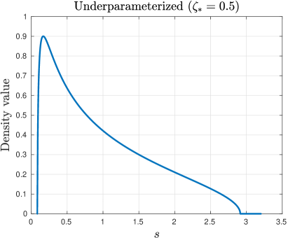
  $$\addcontentsline{lla}{section}{\numberline{\string\crtrefnumber{eq:MP-law-le1}}{e}q:MP-law-le1}\frac{\mathrm{d}F_{\zeta_{\ast}}(s)}{\mathrm{d}s}=\frac{1}{2\pi\zeta_{\ast}s}\sqrt{(b-s)(s-a)}\cdot\operatorname{\mathds{1}}_{[a,b]}(s).$$ (E.6)

  The density is supported on $[a,b]$, where $a=(1-\sqrt{\zeta_{\ast}})^{2}$ and $b=(1+\sqrt{\zeta_{\ast}})^{2}$.

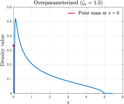
• Overparameterized. For $\zeta_{\ast}>1$, the law $F_{\zeta_{\ast}}$ has an additional point mass at 0 of probability $1-1/\zeta_{\ast}$. In other words,

  $$\addcontentsline{lla}{section}{\numberline{\string\crtrefnumber{eq:MP-law-gt1}}{e}q:MP-law-gt1}\frac{\mathrm{d}F_{\zeta_{\ast}}(s)}{\mathrm{d}s}=\left(1-\frac{1}{\zeta_{\ast}}\right)\delta_{0}(s)+\frac{1}{2\pi\zeta_{\ast}s}\sqrt{(b-s)(s-a)}\cdot\operatorname{\mathds{1}}_{[a,b]}(s).$$ (E.7)

  Here, $\delta_{0}$ is the Dirac delta function at $0$.

We will use some properties of the Marchenko-Pastur law in our proofs. For some visual illustrations in this section, we will values of $\zeta_{\ast}=0.5$ and $\zeta_{\ast}=1.5$ in the underparameterized and overparameterized regimes, respectively. We recall in Figure S.1 the corresponding density plots for these two values of $\zeta_{\ast}$.

Figure S.1: Illustration of the Marchenko-Pastur density in the underparameterized (left) and overparameterized regimes (right). Note that in the overparameterized regime, there is a point mass at $s=0$ (shown with a red dot) as in (E.7). This point mass will need special care in the subsequent asymptotic limits.

Lemma 10 (Risk limit for gradient flow).

Under the assumptions of Theorem 1,

$$R(\widehat{\beta}_{T}^{\mathrm{gf}})\xrightarrow{\mathrm{a.s.}}r^{2}\int\exp(-2Tz)\,\mathrm{d}F_{\zeta_{\ast}}(z)+\zeta_{\ast}\sigma^{2}\int z^{-1}(1-\exp(-Tz))^{2}\,\mathrm{d}F_{\zeta_{\ast}}(z)+\sigma^{2}.$$

Lemma 11 (GCV limit for gradient flow).

Under the assumptions of Theorem 1,

$$\widehat{R}^{\mathrm{gcv}}(\widehat{\beta}_{k})\xrightarrow{\mathrm{a.s.}}\frac{\displaystyle r^{2}\int z\exp(-2Tz)\mathrm{d}F_{\zeta_{\ast}}(z)+\sigma^{2}(1-\zeta_{\ast})+\sigma^{2}\zeta_{\ast}\int\exp(-2Tz)\,\mathrm{d}F_{\zeta_{\ast}}(z)}{\displaystyle\left(1-\zeta_{\ast}\int(1-\exp(-Tz))\,\mathrm{d}F_{\zeta_{\ast}}(z)\right)^{2}}.$$

The proofs of these asymptotic limits in Lemmas 10 and 11 are provided in Sections S.3.4 and S.3.5, respectively.

S.1.3 Step 3: Limits mismatch

The final step involves showing a mismatch between the asymptotics of risk and GCV for gradient flow.

Lemma 12 (Limits mismatch).

Let $F_{\zeta_{\ast}}$ be the Marchenko-Pastur law. Then, assuming either $r^{2}>0$ or $\sigma^{2}>0$, for all $T>0$, except for a set of Lebesgue measure zero,

$$r^{2}\int\exp(-2Tz)\,\mathrm{d}F_{\zeta_{\ast}}(z)+\zeta_{\ast}\sigma^{2}\int z^{-1}(1-\exp(-Tz))^{2}\,\mathrm{d}F_{\zeta_{\ast}}(z)+\sigma^{2}$$

$$\quad\neq\frac{\displaystyle r^{2}\int z\exp(-2Tz)\mathrm{d}F_{\zeta_{\ast}}(z)+\sigma^{2}(1-\zeta_{\ast})_{+}+\sigma^{2}\zeta_{\ast}\int\exp(-2Tz)\,\mathrm{d}F_{\zeta_{\ast}}(z)}{\displaystyle\left(1-\zeta_{\ast}\int(1-\exp(-Tz))\,\mathrm{d}F_{\zeta_{\ast}}(z)\right)^{2}}.\addcontentsline{lla}{section}{\numberline{\string\crtrefnumber{eq:risk_gcv_asymp_mismatch}}{e}q:risk_{g}cv_{a}symp_{m}ismatch}$$ (E.8)

The proof of this asymptotic mismatch in Lemma 12 is provided in Section S.3.6.

Appendix S.2 Supporting lemmas for the proof of Theorem 1

S.2.1 Connections between gradient descent and gradient flow

We first show that under the conditions of Theorem 1, estimates obtained from gradient descent (GD) are in some sense asymptotically equivalent to that obtained from gradient flow (GF).

We next establish connections between GD and GF. This step is achieved by showing that the hat matrices as defined in Equation E.5 when $k\to\infty$ and $k\delta\to T$ (for $H_{k}$) and when $t=T$ (for $H_{t}$) get closer under the matrix operator norm.

Observe that the two matrices in Equation E.5 share a common set of eigenvectors, and the eigenvalues are obtained by applying separate scalar transformations to the eigenvalues of $\widehat{\Sigma}$. Hence, to show that $H_{k}$ and $H_{T}^{\mathrm{gf}}$ are close in terms of operator norm, a natural first step is to show that the scalar transformations are uniformly close to each other. We characterize such closeness in Lemma 13 below.

Let $g_{\delta,k}(x)=\sum_{j=0}^{k-1}\delta x(1-\delta x)^{k-j-1}$ and $g_{T}(x)=1-\exp(-tx)$, which are exactly the scalar transformations of the hat matrices in Equation E.5. Our next lemma says that as $k\to\infty$ and $\delta\to 0$ with $k\delta\to T$, $g_{\delta,k}$ uniformly approximates $g_{T}$ on a compact interval.

Lemma 13 (Scalar uniform approximation for GD and GF smoothing functions).

We assume $k\to\infty$, $\delta\to 0$, and $k\delta\to T$. Here, $T$ is a fixed positive constant. Then it holds that

$$\sup_{0\leq x\leq\zeta_{\ast}+2\sqrt{\zeta_{\ast}}+2}\Big{|}g_{\delta,k}(x)-g_{T}(x)\Big{|}\to 0,$$

where we recall that $\zeta_{\ast}$ is the limit of the aspect ratio.

Proof.

For notational simplicity, we let $J_{\zeta_{\ast}}=[\,0,\zeta_{\ast}+2\sqrt{\zeta_{\ast}}+2\,]$. We will first show that

$$\addcontentsline{lla}{section}{\numberline{\string\crtrefnumber{eq:uniform1}}{e}q:uniform1}\sup_{x\in J_{\zeta_{\ast}}}\Big{|}k\log(1-\delta x)+k\delta x\Big{|}\to 0.$$ (E.9)

To this end, we consider the first-order derivatives of the function inside the above absolute value sign with respect to $x$, which gives $-\delta k/(1-\delta x)+k\delta$. This quantity under the current conditions goes to zero uniformly for all $x\in J_{\zeta_{\ast}}$, thus proving Equation E.9. This further implies the following uniform convergence result:

$$\sup_{x\in J_{\zeta_{\ast}},j+1\in[k]}\Big{|}(k-j-1)\log(1-\delta x)+(k-j-1)\delta\Big{|}\to 0.$$

As a direct consequence of the above equation, we obtain

$$\sup_{x\in J_{\zeta_{\ast}},j+1\in[k]}\Big{|}(1-\delta x)^{k-j-1}-\exp(-\delta(k-j-1)x)\Big{|}\to 0,$$

which further gives

$$\sup_{x\in J_{\zeta_{\ast}}}\Big{|}\sum_{j=0}^{k-1}\delta x(1-\delta x)^{k-j-1}-\sum_{j=0}^{k-1}\delta x\exp(-\delta(k-j-1)x)\Big{|}\to 0$$

as $\sum_{j=0}^{k-1}\delta x$ is uniformly upper bounded for all $x\in J_{\zeta_{\ast}}$.

Considering the derivative of an exponential function, it is not hard to see that

$$\sup_{j+1\in[k]}\sup_{(k-j-1)\delta\leq z\leq(k-j)\delta}\Big{|}\exp(-\delta(k-j-1)x)-\exp(-zx)\Big{|}\to 0.$$

Therefore,

$$\sup_{x\in J_{\zeta_{\ast}}}\Big{|}\sum_{j=0}^{k-1}\delta x\exp(-\delta(k-j-1)x)-\int_{0}^{k\delta}x\exp(-zx)\,\mathrm{d}z\Big{|}\to 0.$$

Further, we note that

$$\sup_{x\in J_{\zeta_{\ast}}}\Big{|}\int_{0}^{k\delta}x\exp(-zx)\,\mathrm{d}z-\int_{0}^{T}x\exp(-zx)\,\mathrm{d}z\Big{|}\to 0$$

and

$$\int_{0}^{T}x\exp(-zx)\,\mathrm{d}z=1-\exp(-Tx).$$

This completes the proof. ∎

We can apply Lemma 13 to establish several useful connections between GD and GF, which we state as Lemmas 9 and 8. The proof of these two lemmas can be found in Appendices S.3.3 and S.3.2, respectively.

S.2.2 Useful concentration results

The following lemma provides the concentration of a linear form of a random vector with independent components. It follows from a moment bound from Lemma 7.8 of Erdos and Yau (2017), along with the Borel-Cantelli lemma and is adapted from Lemma S.8.5 of Patil et al. (2022a).

Lemma 14 (Concentration of linear form with independent components).

Let $z_{p}\in\mathbb{R}^{p}$ be a sequence of random vector with i.i.d. entries $z_{pi}$, $i=1,\dots,p$ such that for each i, $\mathbb{E}[z_{pi}]=0$, $\mathbb{E}[z_{pi}^{2}]=1$, $\mathbb{E}[|z_{pi}|^{4+\alpha}]\leq M_{\alpha}$ for some $\alpha>0$ and constant $M_{\alpha}<\infty$. Let $a_{p}\in\mathbb{R}^{p}$ be a sequence of random vectors independent of $z_{p}$ such that $\limsup_{p}\|a_{p}\|_{2}^{2}/p\leq M_{0}$ almost surely for a constant $M_{0}<\infty$. Then $a_{p}^{\top}z_{p}/p\to 0$ almost surely as $p\to\infty$.

The following lemma provides the concentration of a quadratic form of a random vector with independent components. It follows from a moment bound from Lemma B.26 of Bai and Silverstein (2010), along with the Borel-Cantelli lemma and is adapted from Lemma S.8.6 of Patil et al. (2022a).

Lemma 15 (Concentration of quadratic form with independent components).

Let $z_{p}\in\mathbb{R}^{p}$ be a sequence of random vector with i.i.d. entries $z_{pi}$, $i=1,\dots,p$ such that for each i, $\mathbb{E}[z_{pi}]=0$, $\mathbb{E}[z_{pi}^{2}]=1$, $\mathbb{E}[|z_{pi}|^{4+\alpha}]\leq M_{\alpha}$ for some $\alpha>0$ and constant $M_{\alpha}<\infty$. Let $D_{p}\in\mathbb{R}^{p\times p}$ be a sequence of random matrix such that $\limsup\|D_{p}\|_{\operatorname{op}}\leq M_{0}$ almost surely as $p\to\infty$ for some constant $M_{0}<\infty$. Then $z_{p}^{\top}D_{p}z_{p}/p-\operatorname{tr}[D_{p}]/p\to 0$ almost surely as $p\to\infty$.

Appendix S.3 Proof of Theorem 1

See 1

S.3.1 Proof schematic

A visual schematic for the proof of Theorem 1 is provided in Figure S.2. The lemmas that appear in the figure shall be introduced in later parts of this section.

Figure S.2: Schematic for the proof of Theorem 1

S.3.2 Proof of Lemma 8

See 8

Proof.

Note that the prediction risks admit the following expressions:

$$R(\widehat{\beta}_{k})=\|\beta_{0}-\widehat{\beta}_{k}\|_{2}^{2}+\sigma^{2}\quad\text{and}\quad R(\widehat{\beta}_{T}^{\mathrm{gf}})=\|\beta_{0}-\widehat{\beta}_{T}^{\mathrm{gf}}\|_{2}^{2}+\sigma^{2}.$$

We define $\bar{g}_{\delta,k}(x)=\sum_{j=0}^{k-1}\delta(1-\delta x)^{k-j-1}$ and $\bar{g}_{T}(x)=x^{-1}(1-\exp(-Tx))$. We claim that

$$\addcontentsline{lla}{section}{\numberline{\string\crtrefnumber{eq:uniform-approximation-bar}}{e}q:uniform-approximation-bar}\|x^{1/2}(\bar{g}_{\delta,k}(x)-\bar{g}_{T}(x))\mathbbm{1}_{x\in J_{\zeta_{\ast}}}\|_{\infty}\to 0$$ (E.10)

under the asymptotics $k\to\infty$, $\delta\to 0$, and $k\delta\to T$. Proof for this claim is similar to that for Lemma 13, and we skip it for the compactness of presentation.

We note that

$$\addcontentsline{lla}{section}{\numberline{\string\crtrefnumber{eq:diff-beta2}}{e}q:diff-beta2}\widehat{\beta}_{k}-\widehat{\beta}_{T}^{\mathrm{gf}}=\frac{1}{\sqrt{n}}V^{\top}\Big{(}\bar{g}_{\delta,k}(\Lambda^{\top}\Lambda)-\bar{g}_{T}(\Lambda^{\top}\Lambda)\Big{)}\Lambda^{\top}U^{\top}y,$$ (E.11)

where we recall that $X/\sqrt{n}=V\Lambda U$ is the spectral decomposition. It is straightforward to obtain the following upper bound:

$$\Big{\|}\Big{(}\bar{g}_{\delta,k}(\Lambda^{\top}\Lambda)-\bar{g}_{T}(\Lambda^{\top}\Lambda)\Big{)}\Lambda^{\top}\Big{\|}_{\operatorname{op}}\leq\sup_{i\in[n]}\big{|}\lambda_{i}^{1/2}(\bar{g}_{\delta,k}(\lambda_{i})-\bar{g}_{T}(\lambda_{i}))\big{|}.$$

Recall that $\max_{i\in[n]}\lambda_{i}\xrightarrow{\mathrm{a.s.}}(1+\sqrt{\zeta_{\ast}})^{2}$, hence the right-hand side of the above equation converges to zero almost surely (using Equation E.10). By the law of large numbers, we obtain $\|y\|_{2}/\sqrt{n}\xrightarrow{\mathrm{a.s.}}\mathbb{E}[y_{1}^{2}]^{1/2}$. Plugging these results into Equation E.11 gives $\|\widehat{\beta}_{k}-\widehat{\beta}_{T}^{\mathrm{gf}}\|_{2}\xrightarrow{\mathrm{a.s.}}0$ as $n,p\to\infty$. Furthermore, by Equations E.3 and E.4 we have

$$\addcontentsline{lla}{section}{\numberline{\string\crtrefnumber{eq:beta-upper-bound-gfgd}}{e}q:beta-upper-bound-gfgd}\begin{split}&\big{\|}\widehat{\beta}_{T}^{\mathrm{gf}}\big{\|}_{2}\leq\max_{i\in[n]}\lambda_{i}^{1/2}\cdot\bar{g}_{T}\Big{(}\max_{i\in[n]}\lambda_{i}\Big{)}\cdot\frac{1}{\sqrt{n}}\|y\|_{2},\\ &\|\widehat{\beta}_{k}\|_{2}\leq\max_{i\in[n]}\lambda_{i}^{1/2}\cdot\bar{g}_{\delta,k}\Big{(}\max_{i\in[n]}\lambda_{i}\Big{)}\cdot\frac{1}{\sqrt{n}}\|y\|_{2}.\end{split}$$ (E.12)

Standard analysis implies that $\sup_{x\in J_{\zeta_{\ast}}}\sqrt{x}\bar{g}_{T}(x)<\infty$ and $\limsup_{k\to\infty,\delta\to 0}\sup_{x\in J_{\zeta_{\ast}}}\sqrt{x}\bar{g}_{\delta,k}(x)<\infty$.

Finally, combining all these results we have obtained, we conclude that

$$\left|\|\beta_{0}-\widehat{\beta}_{k}\|_{2}^{2}-\|\beta_{0}-\widehat{\beta}_{T}^{\mathrm{gf}}\|_{2}^{2}\right|\xrightarrow{\mathrm{a.s.}}0$$

as $n,p\to\infty$. This is equivalent to saying

$$|R(\widehat{\beta}_{k})-R(\widehat{\beta}_{T}^{\mathrm{gf}})|\xrightarrow{\mathrm{a.s.}}0$$

as $n,p\to\infty$. ∎

S.3.3 Proof of Lemma 9

See 9

Proof.

In the sequel, we will apply Lemma 13 to prove closeness between $\widehat{R}^{\mathrm{gcv}}(\widehat{\beta}_{k})$ and $\widehat{R}^{\mathrm{gcv}}(\widehat{\beta}_{T}^{\mathrm{gf}})$. This consists of proving the following three pairs of quantities are close:

• $(1-\operatorname{tr}(H_{k})/n)^{-2}$ and $(1-\operatorname{tr}(H_{T}^{\mathrm{gf}})/n)^{-2}$.

• $\widehat{\beta}_{k}^{\top}\widehat{\Sigma}\widehat{\beta}_{k}$ and $(\widehat{\beta}_{T}^{\mathrm{gf}})^{\top}\widehat{\Sigma}\widehat{\beta}_{T}^{\mathrm{gf}}$.

• $y^{\top}X\widehat{\beta}_{k}/n$ and $y^{\top}X\widehat{\beta}_{T}^{\mathrm{gf}}/n$.

In what follows, we shall separately justify each of these closeness results.

Closeness result (1)

We denote by $\{\lambda_{i}\}_{i\leq n}$ the top $n$ eigenvalues of $\widehat{\Sigma}$. From Bai and Silverstein (2010, Theorem 5.8), we know that $\max_{i\in[n]}\lambda_{i}\xrightarrow{\mathrm{a.s.}}(1+\sqrt{\zeta_{\ast}})^{2}$. Note that

$$\frac{1}{n}\operatorname{tr}(H_{k})=\frac{1}{n}\sum_{i=1}^{n}g_{\delta,k}(\lambda_{i})\quad\text{and}\quad\frac{1}{n}\operatorname{tr}(H_{T}^{\mathrm{gf}})=\frac{1}{n}\sum_{i=1}^{n}g_{T}(\lambda_{i}).$$

Invoking Lemma 13, we obtain that with probability one

$$\limsup_{n,p\to\infty}\frac{1}{n}\left|\operatorname{tr}(H_{k})-\operatorname{tr}(H_{T}^{\mathrm{gf}})\right|\leq\sup_{0\leq x\leq\zeta_{\ast}+2\sqrt{\zeta_{\ast}}+2}\Big{|}g_{\delta,k}(x)-g_{T}(x)\Big{|},$$

which vanishes as $n,p\to\infty$. As a result, we derive that $|\operatorname{tr}(H_{k})-\operatorname{tr}(H_{T}^{\mathrm{gf}})|/n\xrightarrow{\mathrm{a.s.}}0$ as $n,p\to\infty$.

Let $F_{\zeta_{\ast}}(s)$ denote the Marchenko-Pasture law as defined in (E.6) and (E.6). Standard results in random matrix theory (Bai and Silverstein, 2010) tell us that the empirical spectral distribution of $\widehat{\Sigma}$ almost surely converges in distribution to $F_{\zeta_{\ast}}$. Note that $g_{T}$ is a bounded continuous function on $[0,\zeta_{\ast}+2\sqrt{\zeta_{\ast}}+2]$, thus

$$\frac{1}{n}\sum_{i=1}^{n}g_{T}(\lambda_{i})\xrightarrow{\mathrm{a.s.}}\int\big{(}1-\exp(-Tz)\big{)}\,\mathrm{d}F_{\zeta_{\ast}}(z),$$

which one can verify is strictly smaller than $1$ for all $\zeta_{\ast}\in(0,\infty)$. Putting together the above analysis, we can deduce that both $(1-\operatorname{tr}(H_{k})/n)^{-2}$ and $(1-\operatorname{tr}(H_{T}^{\mathrm{gf}})/n)^{-2}$ converge almost surely to one finite constant, hence concluding the proof for this part.

Closeness result (2)

We denote by $X/\sqrt{n}=U\Lambda V$ the singular value decomposition of $X/\sqrt{n}$, where $U\in\mathbb{R}^{n\times n}$ and $V\in\mathbb{R}^{p\times p}$ are orthogonal matrices. Combining Equations E.3 and E.4, we arrive at the following equation:

$$\addcontentsline{lla}{section}{\numberline{\string\crtrefnumber{eq:close2}}{e}q:close2}\widehat{\beta}_{k}^{\top}\widehat{\Sigma}\widehat{\beta}_{k}-(\widehat{\beta}_{T}^{\mathrm{gf}})^{\top}\widehat{\Sigma}\widehat{\beta}_{T}^{\mathrm{gf}}=y^{\top}U^{\top}\cdot\left\{g_{\delta,k}(\Lambda\Lambda^{\top})^{2}-g_{T}(\Lambda\Lambda^{\top})^{2}\right\}\cdot Uy/n.$$ (E.13)

By the strong law of large numbers, we have $\|y\|_{2}^{2}/n\xrightarrow{\mathrm{a.s.}}\mathbb{E}[y_{1}^{2}]$. By Lemma 13 and the fact that $\max_{i\in[n]}\lambda_{i}\xrightarrow{\mathrm{a.s.}}(1+\sqrt{\zeta_{\ast}})^{2}$, we conclude that

$$\big{\|}g_{\delta,k}(\Lambda\Lambda^{\top})^{2}-g_{T}(\Lambda\Lambda^{\top})^{2}\big{\|}_{\operatorname{op}}\xrightarrow{\mathrm{a.s.}}0.$$

Plugging these arguments into Equation E.13, we obtain

$$\left|\widehat{\beta}_{k}^{\top}\widehat{\Sigma}\widehat{\beta}_{k}-(\widehat{\beta}_{T}^{\mathrm{gf}})^{\top}\widehat{\Sigma}\widehat{\beta}_{T}^{\mathrm{gf}}\right|\xrightarrow{\mathrm{a.s.}}0,$$

which concludes the proof of closeness result (2).

Closeness result (3)

Finally, we show one more closeness result (3). We note that

$$\frac{1}{n}\big{(}y^{\top}X\widehat{\beta}_{k}-y^{\top}X\widehat{\beta}_{T}^{\mathrm{gf}}\big{)}=y^{\top}U^{\top}\cdot\left\{g_{\delta,k}(\Lambda\Lambda^{\top})-g_{T}(\Lambda\Lambda^{\top})\right\}\cdot Uy/n,$$

which by the same argument as that we used to derive result (2) almost surely converges to zero as $n,p\to\infty$.

Putting together (1), (2), and (3), we conclude the proof of the lemma. ∎

S.3.4 Proof of Lemma 10

See 10

Proof.

Applying Equation E.3 and the risk decomposition formula, we obtain

$$R(\widehat{\beta}_{T}^{\mathrm{gf}})= \beta_{0}^{\top}\exp(-2T\widehat{\Sigma})\beta_{0}-\frac{2}{n}\beta_{0}^{\top}\exp(-T\widehat{\Sigma})\widehat{\Sigma}^{\dagger}({I}_{p}-\exp(-T\widehat{\Sigma}))X^{\top}\varepsilon$$

$$+\frac{1}{n^{2}}\varepsilon^{\top}X({I}_{p}-\exp(-T\widehat{\Sigma}))(\widehat{\Sigma}^{\dagger})^{2}({I}_{p}-\exp(-T\widehat{\Sigma}))X^{\top}\varepsilon+\sigma^{2}.$$

Note that

$$\frac{2}{\sqrt{n}}\big{\|}\beta_{0}^{\top}\exp(-T\widehat{\Sigma})\widehat{\Sigma}^{\dagger}({I}_{p}-\exp(-T\widehat{\Sigma}))X^{\top}\big{\|}_{2}\leq 2\|\beta_{0}\|_{2}\cdot\sup_{i\in[n]}\frac{\exp(-T\lambda_{i})(1-\exp(-T\lambda_{i}))}{\lambda_{i}^{1/2}},$$

where it is understood that $\lambda^{-1/2}e^{-T\lambda}(1-e^{-T\lambda})\mid_{\lambda=0}=0$. Recall that $\max_{i}\lambda_{i}\xrightarrow{\mathrm{a.s.}}(1+\sqrt{\zeta_{\ast}})^{2}$ and $\|\beta_{0}\|_{2}^{2}\to r^{2}$. Hence, there exists a constant $M_{0}$ such that almost surely

$$\limsup_{n,p\to\infty}\|\beta_{0}^{\top}\exp(-T\widehat{\Sigma})\widehat{\Sigma}^{\dagger}({I}_{p}-\exp(-T\widehat{\Sigma}))X^{\top}\|_{2}^{2}/n\leq M_{0}.$$

Therefore, we can apply Lemma 14 and deduce that

$$\addcontentsline{lla}{section}{\numberline{\string\crtrefnumber{eq:ccc1}}{e}q:ccc1}\frac{2}{n}\beta_{0}^{\top}\exp(-T\widehat{\Sigma})\widehat{\Sigma}^{\dagger}({I}_{p}-\exp(-T\widehat{\Sigma}))X^{\top}\varepsilon\xrightarrow{\mathrm{a.s.}}0.$$ (E.14)

By Lemma 15, we have

$$\left|n^{-2}\varepsilon^{\top}X({I}_{p}-\exp(-T\widehat{\Sigma}))(\widehat{\Sigma}^{\dagger})^{2}({I}_{p}-\exp(-T\widehat{\Sigma}))X^{\top}\varepsilon\right.$$

$$\quad\left.-n^{-2}\sigma^{2}\operatorname{tr}(X({I}_{p}-\exp(-T\widehat{\Sigma}))(\widehat{\Sigma}^{\dagger})^{2}({I}_{p}-\exp(-T\widehat{\Sigma}))X^{\top})\right|\xrightarrow{\mathrm{a.s.}}0.$$

Standard random matrix theory result implies that almost surely the empirical spectral distribution of $\widehat{\Sigma}$ converges in distribution to $F_{\zeta_{\ast}}$, which is the Marchenko-Pastur law defined in (E.6) and (E.7). Furthermore, $\|\widehat{\Sigma}\|_{\operatorname{op}}\xrightarrow{\mathrm{a.s.}}(1+\sqrt{\zeta_{\ast}})^{2}$. Therefore, we conclude that

$$n^{-2}\sigma^{2}\operatorname{tr}(X({I}_{p}-\exp(-T\widehat{\Sigma}))(\widehat{\Sigma}^{\dagger})^{2}({I}_{p}-\exp(-T\widehat{\Sigma}))X^{\top})$$

$$\xrightarrow{\mathrm{a.s.}}\zeta_{\ast}\sigma^{2}\int z^{-1}(1-\exp(-Tz))^{2}\,\mathrm{d}F_{\zeta_{\ast}}(z).$$ (E.15)

Finally, we study the limit of $\beta_{0}^{\top}\exp(-2T\widehat{\Sigma})\beta_{0}$. Let $\Omega\in\mathbb{R}^{p\times p}$ be a uniformly distributed orthogonal matrix that is independent of anything else. Since by assumption $\|\beta_{0}\|_{2}\to r$, we can then couple $\Omega\beta_{0}$ with $g\sim\mathcal{N}(\mathbf{0},\mathbf{I}_{p})$, so that (1) $g$ is independent of $\widehat{\Sigma}$, and (2) $\|\Omega\beta_{0}-rg/\sqrt{p}\|_{2}\xrightarrow{\mathrm{a.s.}}0$. Note that all eigenvalues of $\exp(-2T\widehat{\Sigma})$ are between $0$ and $1$, hence

$$\left|\beta_{0}^{\top}\exp(-2T\widehat{\Sigma})\beta_{0}-\frac{r^{2}}{p}g^{\top}\exp(-2T\widehat{\Sigma})g\right|\xrightarrow{\mathrm{a.s.}}0.$$

Leveraging Lemma 15, we obtain

$$r^{2}g^{\top}\exp(-2T\widehat{\Sigma})g/p\xrightarrow{\mathrm{a.s.}}r^{2}\int\exp(-2Tz)\,\mathrm{d}F_{\zeta_{\ast}}(z).$$

Combining this with (E.14) and (S.3.4), we finish the proof. ∎

S.3.5 Proof of Lemma 11

See 11

Proof.

We separately discuss the numerator and the denominator. We start with the denominator. Recall that the empirical spectral distribution of $\widehat{\Sigma}$ almost surely converges to $F_{\zeta_{\ast}}$ and $\|\widehat{\Sigma}\|_{\operatorname{op}}\xrightarrow{\mathrm{a.s.}}(1+\sqrt{\zeta_{\ast}})^{2}$. Hence,

$$\addcontentsline{lla}{section}{\numberline{\string\crtrefnumber{eq:ccc2.5}}{e}q:ccc2.5}(1-\operatorname{tr}(H_{T}^{\mathrm{gf}})/n)^{-2}\xrightarrow{\mathrm{a.s.}}\left(1-\zeta_{\ast}\int(1-\exp(-Tz))\,\mathrm{d}F_{\zeta_{\ast}}(z)\right)^{-2}.$$ (E.16)

Next, we consider the numerator. Straightforward computation implies that

$$\frac{1}{n}\|y-X\widehat{\beta}_{T}^{\mathrm{gf}}\|_{2}^{2}= \beta_{0}^{\top}\exp(-T\widehat{\Sigma})\widehat{\Sigma}\exp(-T\widehat{\Sigma})\beta_{0}+\frac{1}{n}\big{\|}\big{(}{I}_{n}-\frac{1}{n}X\widehat{\Sigma}^{\dagger}({I}_{p}-\exp(-T\widehat{\Sigma}))X^{\top}\big{)}\varepsilon\big{\|}_{2}^{2}$$

$$+\frac{2}{n}\big{\langle}\beta_{0},\exp(-T\widehat{\Sigma})X^{\top}\big{(}{I}_{n}-\frac{1}{n}X\widehat{\Sigma}^{\dagger}({I}_{p}-\exp(-T\widehat{\Sigma}))X^{\top}\big{)}\varepsilon\big{\rangle}.$$

Since $\|\widehat{\Sigma}\|_{\operatorname{op}}\xrightarrow{\mathrm{a.s.}}(1+\sqrt{\zeta_{\ast}})^{2}$, we then obtain almost surely

$$\limsup_{n,p\to\infty}\big{\|}\exp(-T\widehat{\Sigma})X^{\top}\big{(}{I}_{n}-\frac{1}{n}X\widehat{\Sigma}^{\dagger}({I}_{p}-\exp(-T\widehat{\Sigma}))X^{\top}\big{)}\big{\|}_{\operatorname{op}}\leq G(\zeta_{\ast})<\infty,$$

where $G(\zeta_{\ast})$ is a function of $\zeta_{\ast}$. Therefore, by Lemma 14, we obtain

$$\addcontentsline{lla}{section}{\numberline{\string\crtrefnumber{eq:ccc3}}{e}q:ccc3}\frac{2}{n}\big{\langle}\beta_{0},\exp(-T\widehat{\Sigma})X^{\top}\big{(}{I}_{n}-\frac{1}{n}X\widehat{\Sigma}^{\dagger}({I}_{p}-\exp(-T\widehat{\Sigma}))X^{\top}\big{)}\varepsilon\big{\rangle}\xrightarrow{\mathrm{a.s.}}0.$$ (E.17)

Using the same argument that we used to compute the limiting expression of $\beta_{0}^{\top}\exp(-T\widehat{\Sigma})\beta_{0}$, we conclude that

$$\addcontentsline{lla}{section}{\numberline{\string\crtrefnumber{eq:ccc4}}{e}q:ccc4}\beta_{0}^{\top}\exp(-T\widehat{\Sigma})\widehat{\Sigma}\exp(-T\widehat{\Sigma})\beta_{0}\xrightarrow{\mathrm{a.s.}}r^{2}\int z\exp(-2Tz)\,\mathrm{d}F_{\zeta_{\ast}}(z).$$ (E.18)

In addition, by Lemma 15, we have

$$\addcontentsline{lla}{section}{\numberline{\string\crtrefnumber{eq:ccc5}}{e}q:ccc5}\frac{1}{n}\big{\|}\big{(}{I}_{n}-\frac{1}{n}X\widehat{\Sigma}^{\dagger}({I}_{p}-\exp(-T\widehat{\Sigma}))X^{\top}\big{)}\varepsilon\big{\|}_{2}^{2}\xrightarrow{\mathrm{a.s.}}\sigma^{2}(1-\zeta_{\ast})+\sigma^{2}\zeta_{\ast}\int\exp(-2Tz)\,\mathrm{d}F_{\zeta_{\ast}}(z).$$ (E.19)

To see the limit in (E.19), we expand the matrix of the quadratic form as follows:

$$(I_{n}-\frac{1}{n}X{\widehat{\Sigma}}^{\dagger}(I_{p}-\exp(-T{\widehat{\Sigma}}))X^{\top})(I_{n}-\frac{1}{n}X{\widehat{\Sigma}}^{\dagger}(I_{p}-\exp(-T{\widehat{\Sigma}}))X^{\top})$$

$$=(I_{n}-\frac{1}{n}X{\widehat{\Sigma}}^{\dagger}(I_{p}-\exp(-T{\widehat{\Sigma}}))X^{\top})-\frac{1}{n}X{\widehat{\Sigma}}^{\dagger}(I_{p}-\exp(-T{\widehat{\Sigma}})X^{\top})(I_{n}-\frac{1}{n}X{\widehat{\Sigma}}^{\dagger}(I_{p}-\exp(-T{\widehat{\Sigma}}))X^{\top})$$

$$=(I_{n}-\frac{1}{n}X{\widehat{\Sigma}}^{\dagger}(I_{p}-\exp(-T{\widehat{\Sigma}}))X^{\top})-\frac{1}{n}X{\widehat{\Sigma}}^{\dagger}(I_{p}-\exp(-T{\widehat{\Sigma}}))(I_{p}-{\widehat{\Sigma}}{\widehat{\Sigma}}^{\dagger}(I_{p}-\exp(-T{\widehat{\Sigma}})))X^{\top}.$$

The normalized (by $n$) trace of the matrix above is

$$1-\zeta_{\ast}\operatorname{tr}[(I_{p}-\exp(-T{\widehat{\Sigma}}))]/p-\zeta_{\ast}\operatorname{tr}[(I_{p}-\exp(-T{\widehat{\Sigma}}))\exp(-T{\widehat{\Sigma}})]/p$$

$$=1-\zeta_{\ast}+\zeta_{\ast}\operatorname{tr}[\exp(-2T{\widehat{\Sigma}})]/p.$$

In the above simplification, we used the fact that

$${\widehat{\Sigma}}{\widehat{\Sigma}}^{\dagger}(I_{p}-\exp(-T{\widehat{\Sigma}}))=(I_{p}-\exp(-T{\widehat{\Sigma}})).$$

This fact follows because ${\widehat{\Sigma}}^{\dagger}{\widehat{\Sigma}}$ is the projection onto the row space of $X$. But the image of $I_{p}-\exp(-t{\widehat{\Sigma}})$ is already in the row space. The limit for (E.19) therefore is

$$\sigma^{2}(1-\zeta_{\ast})+\sigma^{2}\zeta_{\ast}\int\exp(-2Tz)\,\mathrm{d}F_{\zeta_{\ast}}(z).$$

We can do quick sanity checks for this limit:

• When $T=0$, we should get $\sigma^{2}$ irrespective of $\zeta_{\ast}$ because we start with a null model.

• When $T=\infty$, we should get the training error of the least squares or ridgeless estimator due to noise. There are two cases:

  • When $\zeta_{\ast}<1$: this is the variance component of the residual of least squares. This should be $\sigma^{2}(1-\zeta_{\ast})$.

  • When $\zeta_{\ast}>1$: this is the variance component of the training error of the ridgeless interpolator, which should be zero.

To check the last point, it is worth noting that

$$\lim_{T\to\infty}\int\exp(-2Tz)\,\mathrm{d}F_{\zeta_{\ast}}(z)=\begin{dcases}0&\zeta_{\ast}<1\\ 1-\frac{1}{\zeta_{\ast}}&\zeta_{\ast}>1.\end{dcases}$$

Now, Equations E.16, E.17, E.18 and E.19 together imply the stated result. ∎

S.3.6 Proof of Lemma 12

See 12

Proof.

Recall the asymptotics of the risk from Lemma 10:

$$R(\widehat{\beta}_{T}^{\mathrm{gf}})$$ (E.20)

$$\xrightarrow{\mathrm{a.s.}}r^{2}\int\exp(-2Tz)\,\mathrm{d}F_{\zeta_{\ast}}(z)+\zeta_{\ast}\sigma^{2}\int z^{-1}(1-\exp(-Tz))^{2}\,\mathrm{d}F_{\zeta_{\ast}}(z)+\sigma^{2}$$

$$=r^{2}\left\{\int\exp(-2Tz)\,\mathrm{d}F_{\zeta_{\ast}}(z)\right\}+\sigma^{2}\left\{1+\zeta_{\ast}\int z^{-1}(1-\exp(-Tz))^{2}\,\mathrm{d}F_{\zeta_{\ast}}(z)\right\}.\addcontentsline{lla}{section}{\numberline{\string\crtrefnumber{eq:risk-asymptotics-bias-var-split}}{e}q:risk-asymptotics-bias-var-split}$$ (E.21)

Recall also the asymptotics of GCV from Lemma 11:

$$\widehat{R}^{\mathrm{gcv}}(\widehat{\beta}_{k})$$ (E.22)

$$\xrightarrow{\mathrm{a.s.}}\frac{\displaystyle r^{2}\int z\exp(-2Tz)\,\mathrm{d}F_{\zeta_{\ast}}(z)+\sigma^{2}(1-\zeta_{\ast})+\sigma^{2}\zeta_{\ast}\int\exp(-2Tz)\,\mathrm{d}F_{\zeta_{\ast}}(z)}{\displaystyle\left(1-\zeta_{\ast}\int(1-\exp(-Tz))\,\mathrm{d}F_{\zeta_{\ast}}(z)\right)^{2}}$$

$$=r^{2}\frac{\displaystyle\int z\exp(-2Tz)\,\mathrm{d}F_{\zeta_{\ast}}(z)}{\displaystyle\left(1-\zeta_{\ast}\int(1-\exp(-Tz))\,\mathrm{d}F_{\zeta_{\ast}}(z)\right)^{2}}+\sigma^{2}\frac{\displaystyle(1-\zeta_{\ast})+\zeta_{\ast}\int\exp(-2Tz)\,\mathrm{d}F_{\zeta_{\ast}}(z)}{\displaystyle\left(1-\zeta_{\ast}\int(1-\exp(-Tz))\,\mathrm{d}F_{\zeta_{\ast}}(z)\right)^{2}}.\addcontentsline{lla}{section}{\numberline{\string\crtrefnumber{eq:gcv-asymptotics-bias-var-split}}{e}q:gcv-asymptotics-bias-var-split}$$ (E.23)

Here, $F_{\zeta_{\ast}}$ is the Marchenko-Pasture law, as defined in (E.6) and (E.7). Observe that both functions (E.21) and (E.23) are analytic (i.e., they can be represented by a convergent power series in a neighborhood of every point in their domain). From the identity theorem for analytic functions (see, e.g., Chapter 1 of Krantz and Parks (2002)), it suffices to show that the functions do not agree in a neighborhood of a point inside the domain. We will do this in the neighborhood of $t=0$. The function value and the derivatives match, but the second derivatives mismatch. This is shown in Sections S.3.6.2 and S.3.6.3. This supplies us with the desired function disagreement and concludes the proof. ∎

A couple of remarks on the proof of Lemma 12 follow.

• Observe that both the risk and the GCV asymptotics in (E.21) and (E.23) split into bias or bias-like and variance or variance-like components, respectively. The bias or bias-like component is scaled by the signal energy, and the variance or variance-like component is scaled by the noise energy. We can also show that except for a set of Lebesgue measure $0$, we have

  $$\int\exp(-2Ts)\,\mathrm{d}F_{\zeta_{\ast}}(s) \neq\frac{\displaystyle\int s\exp(-2Ts)\,\mathrm{d}F_{\zeta_{\ast}}(s)}{\displaystyle\left(1-\zeta_{\ast}\int(1-\exp(-Ts))\,\mathrm{d}F_{\zeta_{\ast}}(s)\right)^{2}},\addcontentsline{lla}{section}{\numberline{\string\crtrefnumber{eq:sig-mismatch}}{e}q:sig-mismatch}$$ (E.24)

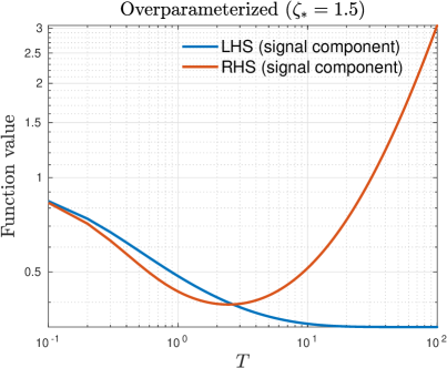
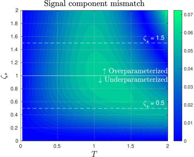
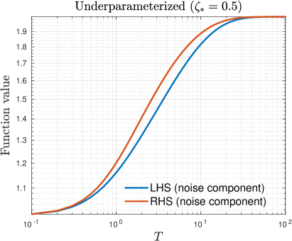
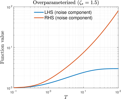
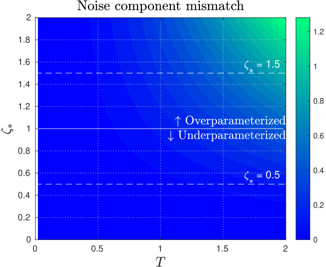
  $$1+\zeta_{\ast}\int\frac{(1-\exp(-Ts))^{2}}{s}\,\mathrm{d}F_{\zeta_{\ast}}(s) \neq\frac{\displaystyle(1-\zeta_{\ast})+\zeta_{\ast}\int\exp(-2Ts)\,\mathrm{d}F_{\zeta_{\ast}}(s)}{\displaystyle\left(1-\zeta_{\ast}\int(1-\exp(-Ts))\,\mathrm{d}F_{\zeta_{\ast}}(s)\right)^{2}}.\addcontentsline{lla}{section}{\numberline{\string\crtrefnumber{eq:var-mismatch}}{e}q:var-mismatch}$$ (E.25)

  In the following, we will refer to (E.24) as the signal component mismatch and (E.25) as the noise component mismatch. The functions on both sides of (E.24) and (E.25) are again analytic in $T$. The mismatch of the second derivatives for the sum above in fact is a consequence of mismatches for the individual signal and noise component. This is shown in Sections S.3.6.2 and S.3.6.3.

• We can also numerically verify the mismatches since the Marchenko-Pasture law has an explicit density as indicated in (E.6) and (E.7). We can simply evaluate both the signal and noise component expressions and observe that the functions are indeed not equal. We numerically illustrate in Sections S.3.6.2 and S.3.6.3 that the functions on the left-hand side and the right-hand side of (E.24) and (E.25) are not equal for the entire range of $T$ plotted (except for when $T=0$).

S.3.6.1 Combined sum mismatch

Our goal is to show that the two limiting functions (of $T$) in (E.21) and (E.23) differ on a neighborhood of $T=0$. Since the common denominator in the two terms in Equation E.23 are away from $0$, it suffices to show that in the neighborhood around $T=0$, the following function is not identically zero:

$$\mathcal{D}(T)= r^{2}\left\{\int\exp(-2Tz)\,\mathrm{d}F_{\zeta_{\ast}}(z)\left(1-\zeta_{\ast}\int(1-\exp(-Tz))\,\mathrm{d}F_{\zeta_{\ast}}(z)\right)^{2}-\int z\exp(-2Tz)\,\mathrm{d}F_{\zeta_{\ast}}(z)\right\}$$

$$+\sigma^{2}\left\{\left(1+\zeta_{\ast}\int z^{-1}(1-\exp(-Tz))^{2}\,\mathrm{d}F_{\zeta_{\ast}}(z)\right)\left(1-\zeta_{\ast}\int(1-\exp(-Tz))\,\mathrm{d}F_{\zeta_{\ast}}(z)\right)^{2}\right.$$

$$\qquad\qquad\left.-(1-\zeta_{\ast})-\zeta_{\ast}\int\exp(-2Tz)\,\mathrm{d}F_{\zeta_{\ast}}(z)\right\}.\addcontentsline{lla}{section}{\numberline{\string\crtrefnumber{eq:diff_risk_gcv_asymp}}{e}q:diff_{r}isk_{g}cv_{a}symp}$$ (E.26)

As argued in the proof of Lemma 12, the function $\mathcal{D}$ is analytic and it suffices to examine the Taylor coefficients. Both $\mathcal{D}(0)$ and $\mathcal{D}^{\prime}(0)$ are $0$ but it turns out that $\mathcal{D}^{\prime\prime}(0)\neq 0$ for $\zeta_{\ast}>0$. Thus, our subsequent goal will be to compute $\mathcal{D}^{\prime\prime}(T)$ and evaluate it at $T=0$. We will make use of double derivative calculations in Sections S.3.6.2 and S.3.6.3 for this purpose, as summarized below.

Claim 16 (Second derivatives mismatch for combined sum).

For the function $\mathcal{D}$ as defined in (E.26), we have $\mathcal{D}^{\prime\prime}(T)=-2\zeta_{\ast}(2r^{2}+\sigma^{2})$. Thus, when $\zeta_{\ast}>0$ and either $r^{2}>0$ or $\sigma^{2}>0$, we have $\mathcal{D}^{\prime\prime}(0)\neq 0$.

Proof.

The calculation follows from Claims 17 and 19. Specifically, using the notation defined in these claims, we have

$$\addcontentsline{lla}{section}{\numberline{\string\crtrefnumber{eq:diff_risk_gcv_asymp_doublederiv}}{e}q:diff_{r}isk_{g}cv_{a}symp_{d}oublederiv}\mathcal{D}^{\prime\prime}(T)=r^{2}(\mathcal{B}^{\prime\prime}_{\ell}(T)-\mathcal{B}^{\prime\prime}_{r}(T))-\sigma^{2}(\mathcal{V}^{\prime\prime}_{\ell}(T)-\mathcal{V}^{\prime\prime}_{r}(T)).$$ (E.27)

Evaluating (E.27) at $T=0$ yields

$$\addcontentsline{lla}{section}{\numberline{\string\crtrefnumber{eq:diff_risk_gcv_asymp_doublederiv_T0}}{e}q:diff_{r}isk_{g}cv_{a}symp_{d}oublederiv_{T}0}\mathcal{D}^{\prime\prime}(0)=r^{2}(4+12\zeta_{\ast}+4\zeta_{\ast}^{2})-r^{2}(4+14\zeta_{\ast}+4\zeta_{\ast}^{2})-\sigma^{2}(4\zeta_{\ast}^{2})+\sigma^{2}(4\zeta_{\ast}+4\zeta_{\ast}^{2}).$$ (E.28)

Simplifying (E.28), we obtain the desired conclusion. ∎

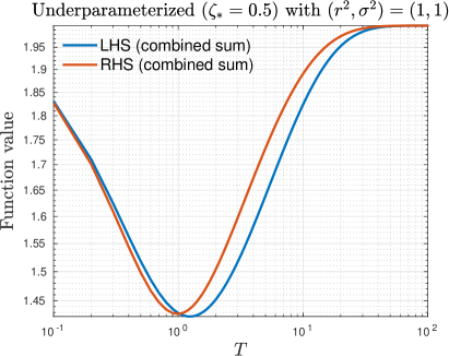
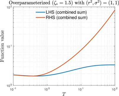
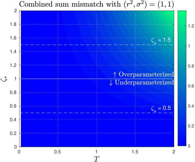
Admittedly, the calculations in Claim 16 are tedious and do not shed much light on the “why”. We also provide numerical illustrations in Figures S.3 and S.4 to help visualize the mismatch for the choice of $(r^{2},\sigma^{2})=(1,1)$. One can also numerically check that the mismatch gets worse as either $r^{2}$ or $\sigma^{2}$ increases. In Section S.11.1, we illustrate this behavior for increasing values of $r^{2}$ and $\sigma^{2}$. While the illustrations may still not illuminate the reason for the mismatch any more than the theoretical calculations just presented, at least they can visually convince the reader of the mismatch. In the figures, we denote $\mathop{\mathrm{SNR}}=r^{2}/\sigma^{2}$.

Figure S.3: Comparison of the LHS and RHS in (E.8) (combined sum) for the underparameterized (left) and overparameterized (right) regimes with $\mathop{\mathrm{SNR}}=1$.

Figure S.4: Contour plot of the absolute value of the difference between LHS and RHS of (E.8) (combined sum) with $\mathop{\mathrm{SNR}}=1$. We observe the mismatch in the north-west corner. In this example, the mismatch is predominantly due to the noise component. See Section S.11.1 for further illustrations where we vary signal energy and noise energy and inspect how the mismatch changes.

S.3.6.2 Signal component mismatch

Claim 17 (Second derivatives mismatch for signal component).

Let $F_{\zeta_{\ast}}$ be the Marchenko-Pasture law as defined in (E.6) and (E.7). Let $\mathcal{B}_{\ell}$ and $\mathcal{B}_{r}$ be two functions defined as follows:

$$\mathcal{B}_{\ell}(T) =\left(1-\zeta_{\ast}\int(1-\exp(-Ts))\,\mathrm{d}F_{\zeta_{\ast}}(s)\right)^{2}\int\exp(-2Ts)\,\mathrm{d}F_{\zeta_{\ast}}(s),$$

$$\mathcal{B}_{r}(T) =\int s\exp(-2Ts)\,\mathrm{d}F_{\zeta_{\ast}}(s).$$

We have $\mathcal{B}^{\prime\prime}_{\ell}(0)=4+12\zeta_{\ast}+4\zeta_{\ast}^{2}$ and $\mathcal{B}^{\prime\prime}_{r}(0)=4+14\zeta_{\ast}+4\zeta_{\ast}^{2}$, and hence $B^{\prime\prime}_{\ell}(0)\neq B^{\prime\prime}_{r}(0)$.

Proof.

For ease of notation, define the functions $w$, $v$, and $u$ as follows:

$$w(T) =\left(1-\zeta_{\ast}\int(1-\exp(-Ts))\,\mathrm{d}F_{\zeta_{\ast}}(s)\right)^{2},$$

$$v(T) =\int\exp(-2Ts)\,\mathrm{d}F_{\zeta_{\ast}}(s),$$

$$u(T) =\int s\exp(-2Ts)\,\mathrm{d}F_{\zeta_{\ast}}(s).$$

Then we have $\mathcal{B}_{\ell}(T)=w(T)v(T)$ and $\mathcal{B}_{r}(T)=u(T)$. The first-order derivatives are $\mathcal{B}^{\prime}_{\ell}(T)=w^{\prime}(T)v(T)+w(T)v^{\prime}(T)$ and $\mathcal{B}^{\prime}_{r}(T)=u^{\prime}(T)$. The second-order derivatives are $\mathcal{B}^{\prime\prime}_{\ell}(T)=w^{\prime\prime}(T)+2w^{\prime}(T)v^{\prime}(T)+v^{\prime\prime}(T)$ and $\mathcal{B}^{\prime\prime}_{r}(T)=u^{\prime\prime}(T)$. From Claim 18, we obtain

$$\mathcal{B}^{\prime\prime}_{\ell}(0)=2\zeta_{\ast}(1+2\zeta_{\ast})+8\zeta_{\ast}+4(1+\zeta_{\ast})=4+14\zeta_{\ast}+4\zeta_{\ast}^{2}.$$

On the other hand, from Claim 18 again, we have

$$\mathcal{B}^{\prime}_{r}(0)=4(1+3\zeta_{\ast}+\zeta_{\ast}^{2})=4+12\zeta_{\ast}+4\zeta_{\ast}^{2}.$$

Thus, for any $\zeta_{\ast}>0$, we have that $\mathcal{B}^{\prime\prime}_{\ell}(0)\neq\mathcal{B}^{\prime\prime}_{r}(0)$, as desired. ∎

Claim 18 (Second derivatives of various parts signal component).

Let $w$, $v$, and $u$ be functions defined in the proof of Claim 17. Then the following claims hold.

• $w(0)=1$, $w^{\prime}(0)=-2\zeta_{\ast}$, and $w^{\prime\prime}(0)=2\zeta_{\ast}(1+2\zeta_{\ast})$.

• $v(0)=1$, $v^{\prime}(0)=-2$, and $v^{\prime\prime}(0)=4(1+\zeta_{\ast})$.

• $u(0)=1$, $u^{\prime}(0)=-2(1+\zeta_{\ast})$, and $u^{\prime\prime}(0)=4(1+3\zeta_{\ast}+\zeta_{\ast}^{2})$.

Proof.

The functional evaluations are straightforward. We will split the first- and second-order derivative calculations into separate parts below. For $k\geq 0$, let $M_{k}=\int s^{k}\,\mathrm{d}F_{\zeta_{\ast}}(s)$ be the $k$-th moment of the Marchenko-Pastur law.

Part 1.

Denote the inner integral by

$$I(T)=\zeta_{\ast}\int(1-\exp(-Ts))\,\mathrm{d}F_{\zeta_{\ast}}(s).$$

Then, $w(T)=(1-I(T))^{2}$. The first derivative of $w(T)$ is

$$w^{\prime}(T)=-2(1-I(T))\cdot I^{\prime}(T)\quad\text{with}\quad I^{\prime}(T)=\zeta_{\ast}\int s\exp(-Ts)\,\mathrm{d}F_{\zeta_{\ast}}(s).$$

The second derivative of $w(T)$ is

$$w^{\prime\prime}(T)=2(I^{\prime}(T))^{2}-2(1-I(T))\cdot I^{\prime\prime}(T)\quad\text{with}\quad I^{\prime\prime}(T)=-\zeta_{\ast}\int s^{2}\exp(-Ts)\,\mathrm{d}F_{\zeta_{\ast}}(s).$$

From (E.29), note that $I(0)=0$, $I^{\prime}(0)=\zeta_{\ast}M_{1}=\zeta_{\ast}$, and $I^{\prime\prime}(0)=-\zeta_{\ast}M_{2}=-\zeta_{\ast}-\zeta_{\ast}^{2}$. Thus, we have $w^{\prime}(0)=-2\zeta_{\ast}M_{1}=-2\zeta_{\ast}$ and $w^{\prime\prime}(0)=2\zeta_{\ast}^{2}+2\zeta_{\ast}+2\zeta_{\ast}^{2}=2\zeta_{\ast}+4\zeta_{\ast}^{2}$.

Part 2.

For $v(T)$, the derivatives are straightforward. The first derivative is

$$v^{\prime}(T)=-2\int s\exp(-2Ts)\,\mathrm{d}F_{\zeta_{\ast}}(s).$$

The second derivative is

$$v^{\prime\prime}(T)=4\int s^{2}\exp(-2Ts)\,\mathrm{d}F_{\zeta_{\ast}}(s).$$

Hence, from (E.29), we then get $v^{\prime}(0)=-2M_{1}=-2$ and $v^{\prime\prime}(0)=4M_{2}=4+4\zeta_{\ast}$.

Part 3.

For $u(T)$, the derivatives are similarly straightforward. The first derivative is

$$u^{\prime}(T)=-2\int s^{2}\exp(-2Ts)\,\mathrm{d}F_{\zeta_{\ast}}(s).$$

The second derivative is

$$u^{\prime\prime}(T)=4\int s^{3}\exp(-2Ts)\,\mathrm{d}F_{\zeta_{\ast}}(s).$$

From Equation E.29 again, we obtain that $u^{\prime}(0)=-2M_{2}=-2(1+\zeta_{\ast})$ and $u^{\prime\prime}(0)=4M_{3}=4(1+3\zeta_{\ast}+\zeta_{\ast})$. ∎

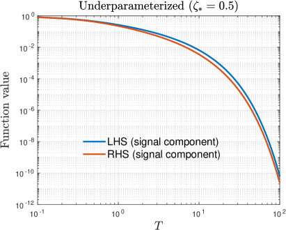
We can also numerically verify that the functions in (E.24) are indeed different in Figures S.5 and S.6.

Figure S.5: Comparison of the LHS and RHS in (E.24) (signal component) for the underparameterized (left) and overparameterized (right) regimes. Note that the signal multiplier for both the regimes at $T=0$ is $1$. This is because the estimator is simply the null estimator at $T=0$, which has bias of $1$.

Figure S.6: Contour plot of the absolute value of the difference between LHS and RHS of (E.24) (signal component).

S.3.6.3 Noise component mismatch

Claim 19 (Second derivatives mismatch for noise component).

Let $F_{\zeta_{\ast}}$ be the Marchenko-Pasture law as defined in (E.6) and (E.7). Let $\mathcal{V}_{\ell}$ and $\mathcal{V}_{r}$ be two functions defined as follows:

$$\mathcal{V}_{\ell}(T) =\left(1+\zeta_{\ast}\int\frac{(1-\exp(-Ts))^{2}}{s}\,\mathrm{d}F_{\zeta_{\ast}}(s)\right)\left(1-\zeta_{\ast}\int(1-\exp(-Ts))\,\mathrm{d}F_{\zeta_{\ast}}(s)\right)^{2}$$

$$\mathcal{V}_{r}(T) ={(1-\zeta_{\ast})+\zeta_{\ast}\int\exp(-2Ts)\,\mathrm{d}F_{\zeta_{\ast}}(s)}.$$

We have $\mathcal{V}^{\prime\prime}_{\ell}(0)=4\zeta_{\ast}^{2}$ and $\mathcal{V}^{\prime\prime}_{r}(0)=4\zeta_{\ast}+4\zeta_{\ast}^{2}$, and hence $\mathcal{V}^{\prime\prime}_{\ell}(0)\neq\mathcal{V}^{\prime\prime}_{r}(0)$ for $\zeta_{\ast}>0$.

Proof.

For ease of notation, define the functions $w$, $\widetilde{v}$, and $\widetilde{u}$ such that

$$w(T) =\left(1-\zeta_{\ast}\int(1-\exp(-Ts))\,\mathrm{d}F_{\zeta_{\ast}}(s)\right)^{2},$$

$$\widetilde{v}(T) =1+\zeta_{\ast}\int\frac{(1-\exp(-Ts))^{2}}{s}\,\mathrm{d}F_{\zeta_{\ast}}(s),$$

$$\widetilde{u}(T) ={(1-\zeta_{\ast})+\zeta_{\ast}\int\exp(-2Ts)\,\mathrm{d}F_{\zeta_{\ast}}(s)}.$$

(Note that the function $w$ is the same function as defined in Claim 18.) Then we have $\mathcal{V}_{\ell}(T)=w(T)\widetilde{v}(T)$ and $\mathcal{V}_{r}(T)=\widetilde{u}(T)$. The first-order derivatives are $\mathcal{V}^{\prime}_{\ell}(T)=w^{\prime}(T)\widetilde{v}(T)+w(T)\widetilde{v}^{\prime}(T)$ and $\mathcal{V}^{\prime}_{r}(T)=\widetilde{u}^{\prime}(T)$. The second-order derivatives are $\mathcal{V}^{\prime\prime}_{\ell}(T)=w^{\prime\prime}(T)+2w^{\prime}(T)\widetilde{v}^{\prime}(T)+\widetilde{v}^{\prime\prime}(T)$ and $\mathcal{V}^{\prime\prime}_{r}(T)=\widetilde{u}^{\prime\prime}(T)$. From Claim 20, we obtain

$$\mathcal{V}^{\prime\prime}_{\ell}(0)=2\zeta_{\ast}(1+2\zeta_{\ast})-2\zeta_{\ast}=4\zeta_{\ast}^{2}.$$

On the other hand, from Claim 20 again, we have

$$\mathcal{V}^{\prime\prime}_{r}(0)=4\zeta_{\ast}+4\zeta_{\ast}^{2}.$$

Thus, we have that $\mathcal{V}^{\prime\prime}_{\ell}(0)\neq\mathcal{V}^{\prime\prime}_{r}(0)$ for any $\zeta_{\ast}>0$. This concludes the proof. ∎

Claim 20 (Second derivatives of various parts of noise component).

Let $w$, $\widetilde{v}$, and $\widetilde{u}$ be functions defined in the proof of Claim 19. Then the following claims hold.

• $w(0)=1$, $w^{\prime}(0)=-2\zeta_{\ast}$, and $w^{\prime\prime}(0)=2\zeta_{\ast}(1+2\zeta_{\ast})$.

• $\widetilde{v}(0)=1$, $\widetilde{v}^{\prime}(0)=0$, and $\widetilde{v}^{\prime\prime}(0)=-2\zeta_{\ast}$.

• $\widetilde{u}(0)=1$, $\widetilde{u}^{\prime}(0)=-2$, and $\widetilde{u}^{\prime\prime}(0)=4(1+\zeta_{\ast})$.

Proof.

The functional evaluations are straightforward. We will split the first- and second-order derivative calculations into separate parts below. Recall that for $k\geq 0$, we denote by $M_{k}=\int s^{k}\,\mathrm{d}F_{\zeta_{\ast}}(s)$ the $k$-th moment of the Marchenko-Pastur law.

Part 1.

This part is the same as Part 1 of Claim 18.

Part 2.

We start by computing the derivative of the integrand.

$$\frac{\partial}{\partial T}\left(\frac{(1-\exp(-Ts))^{2}}{s}\right)=2(1-\exp(-Ts))\cdot(-\exp(-Ts))\cdot(-s)\cdot\frac{1}{s}=2(1-\exp(-Ts))\exp(-Ts)$$

For the second derivative, note that

$$\frac{\partial^{2}}{\partial T^{2}}\left(\frac{(1-\exp(-Ts))^{2}}{s}\right)=\frac{\partial}{\partial T}(2(1-\exp(-Ts))\exp(-Ts))=-2s\exp(-Ts)+4s\exp(-2Ts).$$

Therefore, we have

$$\widetilde{v}^{\prime}(T)=2\zeta_{\ast}\int(1-\exp(-Ts))\exp(-Ts)\,\mathrm{d}F_{\zeta_{\ast}}(s)$$

and

$$\widetilde{v}^{\prime\prime}(T)=2\zeta_{\ast}\int s\exp(-Ts)(1-2\exp(-Ts))\,\mathrm{d}F_{\zeta_{\ast}}(s).$$

Thus, $\widetilde{v}^{\prime}(0)=0$ and $\widetilde{v}^{\prime\prime}(0)=-2\zeta_{\ast}M_{1}=-2\zeta_{\ast}$.

Part 3.

For $\widetilde{u}(T)$, the derivatives are straightforward. The first derivative is

$$\widetilde{u}^{\prime}(T)=-2\zeta_{\ast}\int s\exp(-2Ts)\,\mathrm{d}F_{\zeta_{\ast}}(s).$$

The second derivative is

$$\widetilde{u}^{\prime\prime}(T)=4\zeta_{\ast}\int s^{2}\exp(-2Ts)\,\mathrm{d}F_{\zeta_{\ast}}(s).$$

From Equation E.29 again, we obtain that $\widetilde{u}^{\prime}(0)=-2\zeta_{\ast}M_{1}=-2\zeta_{\ast}$ and $\widetilde{u}^{\prime\prime}(0)=4\zeta_{\ast}M_{2}=4\zeta_{\ast}(1+\zeta_{\ast})$. ∎

We numerically verify that the functions are indeed different in Figures S.7 and S.8.

Figure S.7: Comparison of the LHS and RHS in (E.25) (noise component) for the underparameterized the (left) and overparameterized (right) regimes.

Figure S.8: Contour plot of the absolute value of the difference between LHS and RHS of (E.25) (noise component).

S.3.7 A helper lemma related to the Marchenko-Pastur law

Lemma 21 (Moments of the Marchenko-Pasture distribution).

Let $F_{\zeta_{\ast}}$ be the Marchenko-Pasture law as defined in (E.6) and (E.7). For $k\geq 1$, we have

$$\int s^{k}\,\mathrm{d}F_{\zeta_{\ast}}(s)=\sum_{i=0}^{k-1}\frac{1}{i+1}\binom{k}{i}\binom{k-1}{i}\zeta_{\ast}^{i}.$$

The explicit moment formula in Lemma 21 is well-known. See, for example, Lemma 3.1 of Bai and Silverstein (2010). It can be derived using the Chu-Vandermonde identity, also known as Vandermonde’s convolutional formula for binomial coefficients (Koepf, 1998, Chapter 3).

We will use Lemma 21 to obtain the following moments explicitly. Let $M_{k}$ denote the $k$-th moment $\int s^{k}\,\mathrm{d}F_{\zeta_{\ast}}(s)$ of the Marchenko-Pastur distribution. We have

$$\addcontentsline{lla}{section}{\numberline{\string\crtrefnumber{eq:mp-moments}}{e}q:mp-moments}M_{0}=1,\quad M_{1}=1,\quad M_{2}=1+\zeta_{\ast},\quad M_{3}=1+3\zeta_{\ast}+\zeta_{\ast}^{2},\quad M_{4}=1+6\zeta_{\ast}+6\zeta_{\ast}^{2}+\zeta_{\ast}^{3}.$$ (E.29)

Appendix S.4 Proof sketch for Theorem 2

In this section, we outline the proof idea of Theorem 2. The extension to general test functionals can be found in Appendix S.8. We will prove both the theorems for a general starting estimator $\widehat{\beta}_{0}$.

S.4.1 Step 1: LOO concentration

The most challenging part of our proof is establishing concentration for $\widehat{R}^{\mathrm{loo}}(\widehat{\beta}_{k})$. This is achieved by upper bounding the norm of the gradient of the mapping $(w_{1},\cdots,w_{n})\mapsto\widehat{R}^{\mathrm{loo}}(\widehat{\beta}_{k})$, where $w_{i}=(x_{i},y_{i})$. Although this mapping is not exactly Lipschitz, it is approximately Lipschitz in the sense that its gradient is bounded on a set that occurs with high probability.

For $k\in\{0\}\cup[K]$, we define $f_{k}:\mathbb{R}^{n(p+2)}\mapsto\mathbb{R}$ as $f_{k}(w_{1},\cdots,w_{n})=\widehat{R}^{\mathrm{loo}}(\widehat{\beta}_{k})$. Our goal is to upper bound $\|\nabla f_{k}\|_{2}$. It will become clear that $f_{k}$ is Lipschitz continuous on a closed convex set $\Omega$. We define $\Omega$ as follows:

$$\addcontentsline{lla}{section}{\numberline{\string\crtrefnumber{eq:Omega}}{e}q:Omega}\Omega=\left\{\|\widehat{\Sigma}\|_{\operatorname{op}}\leq C_{\Sigma,\zeta},\,\|y\|_{2}^{2}\leq n(m+\log n)\right\},$$ (E.30)

where $C_{\Sigma,\zeta}=2C_{0}\sigma_{\Sigma}(1+\zeta)+1$, $m=m_{2}$, and $C_{0}>0$ is a numerical constant. It can be verified that $\Omega$ is a convex set of the data. Standard concentration results (see Lemma 29 and Lemma 30) imply that with an appropriately selected $C_{0}$, we have $\mathbb{P}(\Omega)\geq 1-2(n+p)^{-4}-n^{-1}m_{4}\log^{-2}n$. In other words, for large $(n,p)$, the input samples will fall inside $\Omega$ with high probability.

In the following, we establish the Lipschitz continuity of ${f}_{k}$ when restricted to $\Omega$, which is a closed convex set. This can be equivalently stated as the Lipschitz continuity of the composition of the projection onto $\Omega$ and $f_{k}$. To prove this, we upper bound the Euclidean norm of the gradient, as detailed in Lemma 22. The proof of Lemma 22 can be found in Appendix S.7.

Lemma 22 (Gradient upper bound).

There exists a constant $\xi(C_{\Sigma,\zeta},\Delta,m,B_{0})>0$ that depends only on $(C_{\Sigma,\zeta},\Delta,m,B_{0})$, such that on the set $\Omega$, it holds that

$$\|\nabla_{W}f_{k}(W)\|_{F}\leq\frac{K\xi(C_{\Sigma,\zeta},\Delta,m,B_{0})\cdot\log n}{\sqrt{n}}$$

for all $k\in\{0\}\cup[K]$. In the above display, we define $W=(w_{1},\cdots,w_{n})$ and $K$, we recall, is the total number of GD iterations.

We define $h:\mathbb{R}^{n(p+2)}\mapsto\mathbb{R}^{n(p+2)}$ as the projection that projects its inputs onto $\Omega$. Define $\widetilde{f}_{k}=f_{k}\circ h$. Lemma 22 implies that $\widetilde{f}_{k}$ is a Lipschitz continuous mapping with a Lipschitz constant as stated in Lemma 22. By assumption, the input data distribution satisfies a $T_{2}$-inequality, allowing us to apply a powerful concentration inequality stated in Proposition 27 to obtain the desired concentration result. We state this result as Lemma 23 below, and its proof can be found in Section S.6.2.

Lemma 23 (LOO concentration).

We assume the assumptions of Theorem 2. Then with probability at least $1-2(n+p)^{-4}-(n\log^{2}n)^{-1}m_{4}-2(K+1)C_{\mathsf{T_{2}}}n^{-2}$, it holds that for all $k\in\{0\}\cup[K]$

$$\left|\widehat{R}^{\mathrm{loo}}(\widehat{\beta}_{k})-\mathbb{E}[\widetilde{f}_{k}(w_{1},\cdots,w_{n})]\right|\leq\frac{2\sigma_{\mathsf{T_{2}}}LK\xi(C_{\Sigma,\zeta},\Delta,m,B_{0})\cdot(\log n)^{3/2}}{\sqrt{n}},$$

where we let $L=(L_{f}^{2}\sigma_{\Sigma}+L_{f}^{2}+\sigma_{\Sigma})^{1/2}$, $\sigma_{\mathsf{T_{2}}}^{2}=\sigma_{z}^{2}\vee\sigma_{\varepsilon}^{2}$, and $C_{\mathsf{T_{2}}}$ is a positive numerical constant that appears in Proposition 27.

S.4.2 Step 2: Risk concentration

In the second part, we provide concentration bounds for the prediction risk $R(\widehat{\beta}_{k})$. We follow a similar approach as in Step 1, establishing that $R(\widehat{\beta}_{k})$ is a Lipschitz function of the input data with high probability. Leveraging the assumption of a $T_{2}$-inequality in the data distribution, we apply Proposition 27 to derive a concentration result. The proof of this result is presented in Section S.6.3. We state the concentration result as Lemma 24.

Lemma 24 (Risk concentration).

We write $R(\widehat{\beta}_{k})=r_{k}(w_{1},\cdots,w_{n})$ and define $\widetilde{r}_{k}(w_{1},\cdots,w_{n})=r_{k}(h(w_{1},\cdots,w_{n}))$. Then under the assumptions of Theorem 2, with probability at least $1-2(n+p)^{-4}-(n\log^{2}n)^{-1}m_{4}-2(K+1)C_{\mathsf{T_{2}}}n^{-2}$, for all $k\in\{0\}\cup[K]$ we have

$$\left|R(\widehat{\beta}_{k})-\mathbb{E}[\widetilde{r}_{k}(w_{1},\cdots,w_{n})]\right|\leq\frac{2\sigma_{\mathsf{T_{2}}}L\bar{\xi}(C_{\Sigma,\zeta},\Delta,m,B_{0})(\log n)^{3/2}}{\sqrt{n}},$$

where $\bar{\xi}(C_{\Sigma,\zeta},\Delta,m,B_{0})>0$ depends uniquely on $(C_{\Sigma,\zeta},\Delta,m,B_{0})$.

S.4.3 Step 3: LOO bias analysis

In Steps 1 and 2, we have proven concentration results for both $R(\widehat{\beta}_{k})$ and $\widehat{R}^{\mathrm{loo}}(\widehat{\beta}_{k})$. Specifically, we have shown that $R(\widehat{\beta}_{k})$ concentrates around $\mathbb{E}[\widetilde{r}_{k}(w_{1},\cdots,w_{n})]$ and $\widehat{R}^{\mathrm{loo}}(\widehat{\beta}_{k})$ concentrates around $\mathbb{E}[\widetilde{f}_{k}(w_{1},\cdots,w_{n})]$. These expectations represent the target functionals composed with the projection $h$.

Next, we demonstrate that incorporating the projection $h$ into the expectation does not significantly alter the quantities of interest. This result is presented as Lemma 25 below.

Lemma 25 (Projection effects).

Under the assumptions of Theorem 2, it holds that

$$\addcontentsline{lla}{section}{\numberline{\string\crtrefnumber{eq:truncation-expectation}}{e}q:truncation-expectation}\begin{split}&\sup_{k\in\{0\}\cup[K]}\left|\mathbb{E}[\widetilde{r}_{k}(w_{1},\cdots,w_{n})]-\mathbb{E}[r_{k}(w_{1},\cdots,w_{n})]\right|=o_{n}(1),\\ &\sup_{k\in\{0\}\cup[K]}\left|\mathbb{E}[\widetilde{f}_{k}(w_{1},\cdots,w_{n})]-\mathbb{E}[f_{k}(w_{1},\cdots,w_{n})]\right|=o_{n}(1).\end{split}$$ (E.31)

Finally, we aim to establish a result showing that the prediction risk is stable with respect to the sample size. Specifically, we seek to demonstrate that $\mathbb{E}[R(\widehat{\beta}_{k})]$ is approximately equal to $\mathbb{E}[R(\widehat{\beta}_{k,-1})]$, which is equivalent to $\mathbb{E}[r_{k}(w_{1},\cdots,w_{n})]\approx\mathbb{E}[f_{k}(w_{1},\cdots,w_{n})]$.

Formally speaking, we prove the following lemma.

Lemma 26 (LOO bias).

Under the assumptions of Theorem 2, it holds that

$$\sup_{k\in\{0\}\cup[K]}\big{|}\mathbb{E}[R(\widehat{\beta}_{k})]-\mathbb{E}[R(\widehat{\beta}_{k,-1})]\big{|}=o_{n}(1).$$

This is equivalently saying

$$\sup_{k\in\{0\}\cup[K]}\big{|}\mathbb{E}[{r}_{k}(w_{1},\cdots,w_{n})]-\mathbb{E}[{f}_{k}(w_{1},\cdots,w_{n})]\big{|}=o_{n}(1).$$

We defer the proofs of Lemma 25 and Lemma 26 to Sections S.6.4 and S.6.5, respectively.

Theorem 2 then follows from these three steps. To be precise, by putting together Lemmas 23, 24, 25 and 26, we obtain that with probability at least $1-4(n+p)^{-4}-2(n\log^{2}n)^{-1}m_{4}-4(K+1)C_{\mathsf{T_{2}}}n^{-2}$, for all $k\in\{0\}\cup[K]$, we have

$$\sup_{k\in\{0\}\cup[K]}\left|R(\widehat{\beta}_{k})-\widehat{R}^{\mathrm{loo}}(\widehat{\beta}_{k})\right|$$

$$\quad\leq\frac{2\sigma_{\mathsf{T_{2}}}LK\xi(C_{\Sigma,\zeta},\Delta,m,B_{0})\cdot(\log n)^{3/2}+2\sigma_{\mathsf{T_{2}}}L\bar{\xi}(C_{\Sigma,\zeta},\Delta,m,B_{0})(\log n)^{3/2}}{\sqrt{n}}.$$ (E.32)

Since $\zeta=p/n$ is both lower and upper bounded, thus we can conclude that

$$\sum_{n=1}^{\infty}\left\{4(n+p)^{-4}+2(n\log^{2}n)^{-1}m_{4}+4(K+1)C_{\mathsf{T_{2}}}n^{-2}\right\}<\infty.$$

Hence, Theorem 2 follows immediately by applying the first Borel–Cantelli lemma. More precisely, we prove that almost surely the event depicted in (S.4.3) occurs only finitely many times.

Appendix S.5 Supporting lemmas for the proofs of Theorems 2, 3 and 4

We present in this section several supporting lemmas that are useful for the analysis presented in Appendix S.6 and Appendix S.7. Without any loss of generality, in this section, we always assume $n\geq 3$, thus $\log n\geq 1$.

S.5.1 Technical preliminaries

We define below what it means for a distribution to satisfy log Sobolev inequality (LSI).

Definition 2 (LSI).

We say a distribution $\mu$ satisfies LSI if there exists a constant $\sigma(\mu)\geq 0$ such that for all smooth function $f$, it holds that

$$\addcontentsline{lla}{section}{\numberline{\string\crtrefnumber{eq:LSI}}{e}q:LSI}\mathrm{Ent}_{w\sim\mu}[f(w)^{2}]\leq 2\sigma^{2}(\mu)\mathbb{E}_{w\sim\mu}\big{[}\|\nabla f(w)\|_{2}^{2}\big{]},$$ (E.33)

where the entropy of a non-negative random variable $Z$ is defined as

$$\mathrm{Ent}[Z]=\mathbb{E}[Z\log Z]-\mathbb{E}[Z]\log\mathbb{E}[Z].$$

S.5.2 Concentration based on $T_{2}$-inequality

In this section, we discuss useful properties of the $T_{2}$-inequality. An important result that will be applied multiple times throughout the proof is Theorem 4.31 of Van Handel (2014), which we include below for the convenience of the readers. See also Gozlan (2009).

Proposition 27 (Equivalent characterizations of $T_{2}$-inequality).

Let $\mu$ be a probability measure on a Polish space $(\mathcal{X},d)$, and let $\{X_{i}\}_{i\leq n}$ be i.i.d. $\sim\mu$. Denote by $d_{n}(x,y)=[\sum_{i=1}^{n}d(x_{i},y_{i})^{2}]^{1/2}$. Then the following are equivalent:

1. $\mu$ satisfies the $T_{2}$-inequality:

   $$W_{2}(\mu,\nu)\leq\sqrt{2\sigma^{2}\mathcal{D}_{\mathrm{\texttt{KL}}}(\nu\,||\,\mu)}\,\,\,\,\mbox{ for all }\nu.$$

2. $\mu^{\otimes n}$ satisfies the $T_{1}$-inequality for every $n\geq 1$:

   $$W_{1}(\mu^{\otimes n},\nu)\leq\sqrt{2\sigma^{2}\mathcal{D}_{\mathrm{\texttt{KL}}}(\nu\,||\,\mu^{\otimes n})}\,\,\,\,\mbox{ for all }\nu\mbox{ and }n\geq 1.$$

3. There is an absolute constant $C_{\mathsf{T_{2}}}$, such that

   $$\addcontentsline{lla}{section}{\numberline{\string\crtrefnumber{eq:LSI-concentration}}{e}q:LSI-concentration}\mathbb{P}\left(f(X_{1},\cdots,X_{n})-\mathbb{E}[f(X_{1},\cdots,X_{n})]\geq t\right)\leq C_{\mathsf{T_{2}}}e^{-t^{2}/2\sigma^{2}}$$ (E.34)

   for every $n\geq 1$, $t\geq 0$ and $1$-Lipschitz function $f$.

S.5.3 Dimension-free concentration

Define $w_{i}=(x_{i},y_{i})$. The following lemma is a straightforward consequence of the assumptions and the $T_{2}$-inequality.

Lemma 28 (Dimension-free concentration).

We let $\sigma_{\mathsf{T_{2}}}^{2}=\sigma_{z}^{2}\vee\sigma_{\varepsilon}^{2}$, and $L=(L_{f}^{2}\sigma_{\Sigma}+L_{f}^{2}+\sigma_{\Sigma})^{1/2}$. Then for any $n\geq 1$, $t\geq 0$, and 1-Lipschitz function $f$, it holds that

$$\mathbb{P}\left(f(w_{1},\cdots,w_{n})-\mathbb{E}[f(w_{1},\cdots,w_{n})]\geq Lt\right)\leq C_{\mathsf{T_{2}}}e^{-t^{2}/2\sigma_{\mathsf{T_{2}}}^{2}},$$

where we recall that $C_{\mathsf{T_{2}}}>0$ is an absolute constant introduced in Proposition 27.

Proof.

Since $f$ is 1-Lipschitz, for any $w_{i},\widetilde{w}_{i}\in\mathbb{R}^{p}$

$$|f(w_{1},\cdots,w_{n})-f(\widetilde{w}_{1},\cdots,\widetilde{w}_{n})|\leq \sqrt{\sum_{i=1}^{n}\|w_{i}-\widetilde{w}_{i}\|_{2}^{2}}$$

$$= \sqrt{\sum_{i=1}^{n}\|x_{i}-\widetilde{x}_{i}\|_{2}^{2}+\sum_{i=1}^{n}|y_{i}-\widetilde{y}_{i}|^{2}}$$

$$\leq \sqrt{\sum_{i=1}^{n}\sigma_{\Sigma}(L_{f}^{2}+1)\|z_{i}-\widetilde{z}_{i}\|_{2}^{2}+\sum_{i=1}^{n}L_{f}^{2}|\varepsilon_{i}-\widetilde{\varepsilon}_{i}|^{2}}$$

$$\leq L\sqrt{\sum_{i=1}^{n}\|z_{i}-\widetilde{z}_{i}\|_{2}^{2}+\sum_{i=1}^{n}|\varepsilon_{i}-\widetilde{\varepsilon}_{i}|^{2}}.$$

Invoking Corollary 4.16 of Van Handel (2014), we obtain that

$$W_{1}(\mu_{z}^{\otimes n}\otimes\mu_{\varepsilon}^{\otimes n},\nu)\leq\sqrt{2\sigma^{2}_{\mathsf{T_{2}}}\mathcal{D}_{\mathrm{\texttt{KL}}}(\nu\,||\,\mu_{z}^{\otimes n}\otimes\mu_{\varepsilon}^{\otimes n})}$$

for all $\nu$. We then see that the desired concentration inequality is a straightforward consequence of Proposition 27. ∎

S.5.4 Upper bounding operator norms and response energy

We then state several technical lemmas required for our analysis. Recall that $\widehat{\Sigma}=X^{\top}X/n$. Our first lemma upper bounds the operator norm of $\widehat{\Sigma}$.

Lemma 29.

We assume the assumptions of Theorem 2. Then there exists a numerical constant $C_{0}>0$, such that with probability at least $1-(n+p)^{-4}$

$$\|\widehat{\Sigma}\|_{\operatorname{op}}\leq 2C_{0}\sigma_{\Sigma}(1+\zeta)+1.$$

Proof.

Note that the operator norm of $\widehat{\Sigma}$ is equal to the operator norm of $Z\Sigma Z^{\top}/n+\mathbf{1}_{n\times n}/n\in\mathbb{R}^{n\times n}$.

To proceed, we will utilize a canonical concentration inequality that bounds the operator norm of random matrices with sub-Gaussian entries. This further requires the introduction of several related concepts.

To be specific, we say a random variable $R$ is sub-Gaussian if and only if there exists $K_{R}>0$ such that $\|R\|_{L^{d}}\leq K_{R}\sqrt{d}$ for all $d\geq 1$. Proposition 2.5.2 of Vershynin (2018) tells us that when such upper bound is satisfied, the sub-Gaussian norm of this random variable $\|Z\|_{\Psi_{2}}$ is no larger than $4K_{R}$.

By Assumption C and Proposition 27, it holds that

$$\mathbb{P}\left(|z_{11}|\geq t\right)\leq 2C_{\mathsf{T_{2}}}e^{-t^{2}/2\sigma_{z}^{2}}.$$

Leveraging the above upper bound and applying an appropriate integral inequality, we can conclude that for all $d\geq 1$,

$$\mathbb{E}[|z_{11}|^{d}]\leq C_{\mathsf{T_{2}}}d(d/2)^{d/2},$$

hence $\|z_{11}\|_{\Psi_{2}}\leq 8+8C_{\mathsf{T_{2}}}$. By Theorem 4.4.5 of Vershynin (2010), we see that for all $t\geq 0$, with probability at least $1-2\exp(-t^{2})$

$$\addcontentsline{lla}{section}{\numberline{\string\crtrefnumber{eq:Zop}}{e}q:Zop}\|Z\|_{\operatorname{op}}\leq C^{\prime}(8+8C_{\mathsf{T_{2}}})(\sqrt{n}+\sqrt{p}+t),$$ (E.35)

where $C^{\prime}>0$ is a numerical constant. Taking $t=2\sqrt{\log(p+n)}$, we conclude that $\|Z\|_{\operatorname{op}}\leq C^{\prime}(8+8C_{\mathsf{T_{2}}})(\sqrt{n}+\sqrt{p}+2\sqrt{\log(n+p)})$ with probability at least $1-2(p+n)^{-4}$. When this occurs, a straightforward consequence is that

$$n\|\widehat{\Sigma}\|_{\operatorname{op}}\leq\|Z\|_{\operatorname{op}}^{2}\|\Sigma\|_{\operatorname{op}}+n\leq C_{0}\sigma_{\Sigma}(n+p+\log(n+p))+n$$

for some positive numerical constant $C_{0}$, thus completing the proof of the lemma. ∎

Our next lemma upper bounds $\|y\|_{2}^{2}/n$. This lemma is a direct consequence of Chebyshev’s inequality, and we skip the proof for the compactness of the presentation.

Lemma 30.

We assume the assumptions of Theorem 2. Then with probability at least $1-n^{-1}m_{4}\log^{-2}n$, we have $\|y\|_{2}^{2}/n\leq m_{2}+\log n$.

S.5.5 Other useful norm bounds

Our next lemma upper bounds the Euclidean norm of $\theta=\mathbb{E}[y_{0}x_{0}]\in\mathbb{R}^{p+1}$, where we recall that $(x_{0},y_{0})\overset{d}{=}(x_{1},y_{1})$.

Lemma 31.

Under the assumptions of Theorem 2, we have $\|\theta\|_{2}\leq(\sigma_{\Sigma}^{1/2}+1)m_{2}^{1/2}$.

Proof.

We notice that

$$\theta=\left(\begin{array}[]{c}\Sigma^{1/2}\mathbb{E}[y_{0}z_{0}]\\ \mathbb{E}[y_{0}]\end{array}\right).$$

We let $x_{0}^{\top}=(z_{0}^{\top}\Sigma^{1/2},1)$. By assumption, $z_{0}$ is isotropic. Hence, $y_{0}$ admits the following decomposition:

$$y_{0}=\sum_{i=1}^{p}\mathbb{E}[y_{0}z_{0,i}]z_{0,i}+\omega,\qquad\mathbb{E}[\omega z_{0,i}]=0\,\,\mbox{ for all }i\in[n].$$

In addition, $\mathbb{E}[y_{0}^{2}]=\mathbb{E}[w^{2}]+\sum_{i\in[p]}\mathbb{E}[y_{0}z_{0,i}]^{2}$. As a result, we are able to deduce that $\|\mathbb{E}[y_{0}z_{0}]\|_{2}\leq m_{2}^{1/2}$, where we recall that $m_{2}=\mathbb{E}[y_{0}^{2}]$. This further tells us $\|\theta\|_{2}\leq\|\Sigma\|_{\operatorname{op}}^{1/2}\times\|\mathbb{E}[y_{0}z_{0}]\|_{2}+m_{2}^{1/2}\leq(\sigma_{\Sigma}^{1/2}+1)m_{2}^{1/2}$, thus completing the proof of the lemma. ∎

We next prove that $\|\widehat{\Sigma}\|_{\operatorname{op}}$ is sub-exponential.

Lemma 32.

We define $\widetilde{C}_{0}=C^{\prime}\sigma_{\Sigma}(8+8C_{\mathsf{T_{2}}})$, where we recall that $C^{\prime}$ is a positive numerical constant that appears in Equation E.35. Under the assumptions of Theorem 2, for all $\lambda\geq 0$ and $n\geq\lambda\widetilde{C}_{0}^{2}+1$, there exists a constant $\mathcal{E}(\widetilde{C}_{0},\zeta,\lambda)>0$ that depends only on $(\widetilde{C}_{0},\zeta,\lambda)$, such that

$$\mathbb{E}[\exp(\lambda\|\widehat{\Sigma}\|_{\operatorname{op}})]\leq\mathcal{E}(\widetilde{C}_{0},\zeta,\lambda).$$

Proof.

By Equation E.35, for all $t\geq 0$, with probability at least $1-2\exp(-nt^{2})$

$$\|\widehat{\Sigma}\|_{\operatorname{op}}^{1/2}=n^{-1/2}\|X\|_{\operatorname{op}}\leq\widetilde{C}_{0}(1+\zeta^{1/2}+t).$$

As a result, for all $\lambda\geq 0$,

$$\mathbb{E}[\exp(\lambda\|\widehat{\Sigma}\|_{\operatorname{op}})]$$

$$\leq 1+\int_{0}^{\infty}2\lambda se^{\lambda s^{2}}\mathbb{P}\Big{(}\|\widehat{\Sigma}\|_{\operatorname{op}}^{1/2}\geq s\Big{)}\mathrm{d}s$$

$$\leq 1+2\lambda\widetilde{C}_{0}^{2}(1+\zeta^{1/2})^{2}e^{\lambda\widetilde{C}_{0}^{2}(1+\zeta^{1/2})^{2}}+\int_{\widetilde{C}_{0}(1+\zeta^{1/2})}2\lambda se^{\lambda s^{2}}\mathbb{P}\Big{(}\|\widehat{\Sigma}\|_{\operatorname{op}}^{1/2}\geq s\Big{)}\mathrm{d}s$$

$$\leq 1+2\lambda\widetilde{C}_{0}^{2}(1+\zeta^{1/2})^{2}e^{\lambda\widetilde{C}_{0}^{2}(1+\zeta^{1/2})^{2}}+\int_{0}^{\infty}4\lambda\widetilde{C}_{0}^{2}(1+\zeta^{1/2}+t)e^{\lambda\widetilde{C}_{0}^{2}(1+\zeta^{1/2}+t)^{2}-nt^{2}}\mathrm{d}t\leq\mathcal{E}(\widetilde{C}_{0},\zeta,\lambda),$$

thus completing the proof of the lemma. ∎

S.5.6 Upper bounding $\|\widehat{\beta}_{k}\|_{2}$ and $\|\widehat{\beta}_{k,-i}\|_{2}$

We then prove that on $\Omega$, the Euclidean norm of the coefficient estimates $\{\widehat{\beta}_{k},\widehat{\beta}_{k,-i}:k\in[K],i\in[n]\}$ are uniformly upper bounded. In addition, apart from a logarithmic factor, this upper bound depends only on the constants from our assumptions and in particular is independent of $(n,p)$.

Lemma 33.

For the sake of simplicity, we let

$$\addcontentsline{lla}{section}{\numberline{\string\crtrefnumber{eq:BstarB}}{e}q:BstarB}B_{\ast}=(B_{0}+\Delta C_{\Sigma,\zeta}^{1/2}\sqrt{m+1})\cdot e^{C_{\Sigma,\zeta}\Delta}.$$ (E.36)

Then on the set $\Omega$, for all $k\in\{0\}\cup[K]$ and $i\in[n]$, it holds that

$$\|\widehat{\beta}_{k}\|_{2}\leq B_{\ast}\sqrt{\log n},\qquad\|\widehat{\beta}_{k,i}\|_{2}\leq B_{\ast}\sqrt{\log n}.$$

Proof.

By definition,

$$\widehat{\beta}_{k+1}= \widehat{\beta}_{k}+\frac{\delta_{k}}{n}\sum_{i=1}^{n}(y_{i}-x_{i}^{\top}\widehat{\beta}_{k})x_{i}$$

$$= \widehat{\beta}_{k}-\delta_{k}\widehat{\Sigma}\widehat{\beta}_{k}+\frac{\delta_{k}}{n}X^{\top}y.$$

Applying the triangle inequality, we obtain the following upper bound:

$$\|\widehat{\beta}_{k+1}\|_{2}\leq \|\widehat{\beta}_{k}\|_{2}+\delta_{k}\|\widehat{\Sigma}\|_{\operatorname{op}}\cdot\|\widehat{\beta}_{k}\|_{2}+\delta_{k}\cdot\|\widehat{\Sigma}\|_{\operatorname{op}}^{1/2}\cdot\|y/\sqrt{n}\|_{2}$$

$$\leq \left(1+\delta_{k}C_{\Sigma,\zeta}\right)\cdot\|\widehat{\beta}_{k}\|_{2}+\delta_{k}C_{\Sigma,\zeta}^{1/2}\sqrt{m+\log n}.$$

By induction, we see that on $\Omega$

$$\|\widehat{\beta}_{k}\|_{2}\leq\left(B_{0}+\Delta C_{\Sigma,\zeta}^{1/2}\sqrt{m+\log n}\right)\cdot e^{C_{\Sigma,\zeta}\Delta}$$

for all $k\in[K]$. The upper bound for $\|\widehat{\beta}_{k,-i}\|_{2}$ follows using exactly the same argument. We complete the proof of the lemma as $\log n\geq 1$. ∎

The following corollary is a straightforward consequence of Lemma 33 and the Cauchy-Schwartz inequality.

Corollary 34.

On the set $\Omega$, it holds that

$$\frac{1}{n}\|y-X\widehat{\beta}_{k,-i}\|_{2}^{2}\leq\Big{(}2m+2+2C_{\Sigma,\zeta}B_{\ast}^{2}\Big{)}\cdot\log n,$$

$$\frac{1}{n}\|y-X\widehat{\beta}_{k}\|_{2}^{2}\leq\Big{(}2m+2+2C_{\Sigma,\zeta}B_{\ast}^{2}\Big{)}\cdot\log n$$

for all $k\in\{0\}\cup[K]$ and $i\in[n]$.

For the compactness of future presentation, we define

$$\addcontentsline{lla}{section}{\numberline{\string\crtrefnumber{eq:BstarBbar}}{e}q:BstarBbar}\bar{B}_{\ast}=(2m+2+2C_{\Sigma,\zeta}B_{\ast}^{2})^{1/2}$$ (E.37)

We comment that both $B_{\ast}$ and $\bar{B}_{\ast}$ depend only on $(C_{\Sigma,\zeta},\Delta,m,B_{0})$.

S.5.7 Upper bounding $|y_{i}-x_{i}^{\top}\beta_{k,-i}|$

We next upper bound $|y_{i}-x_{i}^{\top}\widehat{\beta}_{k,-i}|$ on $\Omega$. More precisely, we shall upper bound collectively the Frobenius norms of

$$a_{k}=(y_{i}-x_{i}^{\top}\widehat{\beta}_{k,-i})_{i=1}^{n}\in\mathbb{R}^{n}\qquad\mbox{and}$$

$$E_{k}=\left[X(\widehat{\beta}_{k}-\widehat{\beta}_{k,-1})\mid\cdots\mid X(\widehat{\beta}_{k}-\widehat{\beta}_{k,-n})\right]\in\mathbb{R}^{n\times n}$$

respectively and recursively. For the base case $k=0$, we have

$$\|a_{0}\|_{2}^{2}\leq\bar{B}_{\ast}^{2}n\log n,\qquad\|E_{0}\|_{F}^{2}=0,$$

where the first upper bound follows from Corollary 34.

Our lemma for this part can be formally stated as follows:

Lemma 35.

We define

$$\mathcal{G}_{1}(C_{\Sigma,\zeta},\Delta,m,B_{0})=\bar{B}_{\ast}\sqrt{e^{3\Delta C_{\Sigma,\zeta}+2\Delta^{2}C_{\Sigma,\zeta}^{2}}(\Delta C_{\Sigma,\zeta}+2\Delta^{2}C_{\Sigma,\zeta}^{2})},\addcontentsline{lla}{section}{\numberline{\string\crtrefnumber{eq:cG1def}}{e}q:cG1def}$$ (E.38)

$$\mathcal{G}_{2}(C_{\Sigma,\zeta},\Delta,m,B_{0})=\bar{B}_{\ast}+\Delta C_{\Sigma,\zeta}\sqrt{8\bar{B}_{\ast}^{2}+2\mathcal{G}_{1}(C_{\Sigma,\zeta},\Delta,m,B_{0})^{2}}.\addcontentsline{lla}{section}{\numberline{\string\crtrefnumber{eq:cG2def}}{e}q:cG2def}$$ (E.39)

Then on the set $\Omega$, for all $k\in\{0\}\cup[K]$ we have

$$\frac{1}{\sqrt{n}}\|E_{k}\|_{F}\leq\mathcal{G}_{1}(C_{\Sigma,\zeta},\Delta,m,B_{0})\cdot\sqrt{\log n},\addcontentsline{lla}{section}{\numberline{\string\crtrefnumber{eq:Ek}}{e}q:Ek}$$ (E.40)

$$\frac{1}{\sqrt{n}}\|a_{k}\|_{2}\leq\mathcal{G}_{2}(C_{\Sigma,\zeta},\Delta,m,B_{0})\cdot\sqrt{\log n}.\addcontentsline{lla}{section}{\numberline{\string\crtrefnumber{eq:ak}}{e}q:ak}$$ (E.41)

Proof.

We first prove Equation E.40. We denote by $X_{-i}\in\mathbb{R}^{(n-1)\times(p+1)}$ the matrix obtained by deleting the $i$-th row from $X$. By definition,

$$X(\widehat{\beta}_{k+1}-\widehat{\beta}_{k+1,-i})= X(\widehat{\beta}_{k}-\widehat{\beta}_{k,-i})+\frac{\delta_{k}(y_{i}-x_{i}^{\top}\widehat{\beta}_{k})}{n}Xx_{i}-\frac{\delta_{k}}{n}X\sum_{j\neq i}x_{j}x_{j}^{\top}(\widehat{\beta}_{k}-\widehat{\beta}_{k,-i})$$

$$= X(\widehat{\beta}_{k}-\widehat{\beta}_{k,-i})+\frac{\delta_{k}(y_{i}-x_{i}^{\top}\widehat{\beta}_{k})}{n}Xx_{i}-\frac{\delta_{k}}{n}XX_{-i}^{\top}X_{-i}(\widehat{\beta}_{k}-\widehat{\beta}_{k,-i}),$$

which further implies

$$\|X(\widehat{\beta}_{k+1}-\widehat{\beta}_{k+1,-i})\|_{2}^{2}$$

$$\leq\left(1+\delta_{k}C_{\Sigma,\zeta}\right)^{2}\|X(\widehat{\beta}_{k}-\widehat{\beta}_{k,-i})\|_{2}^{2}+\frac{\delta_{k}^{2}(y_{i}-x_{i}^{\top}\widehat{\beta}_{k})^{2}}{n^{2}}\|Xx_{i}\|_{2}^{2}$$

$$\quad+\frac{2\delta_{k}(1+\delta_{k}C_{\Sigma,\zeta})\cdot|y_{i}-x_{i}^{\top}\widehat{\beta}_{k}|}{n}\|X(\widehat{\beta}_{k}-\widehat{\beta}_{k,-i})\|_{2}\cdot\|Xx_{i}\|_{2}$$

$$\leq\left(1+\delta_{k}C_{\Sigma,\zeta}\right)^{2}\|X(\widehat{\beta}_{k}-\widehat{\beta}_{k,-i})\|_{2}^{2}+\delta_{k}^{2}C_{\Sigma,\zeta}^{2}(y_{i}-x_{i}^{\top}\widehat{\beta}_{k})^{2}$$

$$\quad+\delta_{k}C_{\Sigma,\zeta}(1+\delta_{k}C_{\Sigma,\zeta})\cdot\big{\{}(y_{i}-x_{i}^{\top}\widehat{\beta}_{k})^{2}+\|X(\widehat{\beta}_{k}-\widehat{\beta}_{k,-i})\|_{2}^{2}\big{\}}$$

$$\leq\big{(}1+3\delta_{k}C_{\Sigma,\zeta}+2\delta_{k}^{2}C_{\Sigma,\zeta}^{2}\big{)}\cdot\|X(\widehat{\beta}_{k}-\widehat{\beta}_{k,-i})\|_{2}^{2}+\big{(}\delta_{k}C_{\Sigma,\zeta}+2\delta_{k}^{2}C_{\Sigma,\zeta}^{2}\big{)}\cdot(y_{i}-x_{i}^{\top}\widehat{\beta}_{k})^{2},$$

where we make use of the fact that $\|Xx_{i}\|_{2}/n\leq C_{\Sigma,\zeta}$ on $\Omega$. Putting together the above upper bound and Corollary 34, then summing over $i\in[n]$, we obtain the following inequality:

$$\|E_{k+1}\|_{F}^{2}\leq\big{(}1+3\delta_{k}C_{\Sigma,\zeta}+2\delta_{k}^{2}C_{\Sigma,\zeta}^{2}\big{)}\cdot\|E_{k}\|_{F}^{2}+\big{(}\delta_{k}C_{\Sigma,\zeta}+2\delta_{k}^{2}C_{\Sigma,\zeta}^{2}\big{)}\cdot\bar{B}_{\ast}^{2}\log n.$$

Employing the standard induction argument, we can conclude that

$$\frac{1}{n}\|E_{k}\|_{F}^{2}\leq e^{3\Delta C_{\Sigma,\zeta}+2\Delta^{2}C_{\Sigma,\zeta}^{2}}(\Delta C_{\Sigma,\zeta}+2\Delta^{2}C_{\Sigma,\zeta}^{2})\cdot\bar{B}_{\ast}^{2}\log n=\mathcal{G}_{1}(C_{\Sigma,\zeta},\Delta,m,B_{0})^{2}\log n$$

for all $k\in\{0\}\cup[K]$. This completes the proof of Equation E.40.

Next, we prove Equation E.41. By definition,

$$y_{i}-x_{i}^{\top}\widehat{\beta}_{k+1,-i}= \,y_{i}-x_{i}^{\top}\widehat{\beta}_{k,-i}-\frac{\delta_{k}}{n}\sum_{j\neq i}(y_{j}-x_{j}^{\top}\widehat{\beta}_{k,-i})x_{i}^{\top}x_{j}$$

$$= \,y_{i}-x_{i}^{\top}\widehat{\beta}_{k,-i}-\frac{\delta_{k}}{n}\sum_{j\neq i}(y_{j}-x_{j}^{\top}\widehat{\beta}_{k})x_{i}^{\top}x_{j}-\frac{\delta_{k}}{n}\sum_{j\neq i}x_{i}^{\top}x_{j}x_{j}^{\top}(\widehat{\beta}_{k}-\widehat{\beta}_{k,-i}).$$

We let $D=\mathop{\mathrm{diag}}\{(\|x_{i}\|_{2}^{2}/n)_{i=1}^{n}\}\in\mathbb{R}^{n\times n}$. We denote by $a_{k,i}$ the $i$-th entry of $a_{k}$. From the above equality, we can deduce that

$$(a_{k+1,i}-a_{k,i})^{2}\leq\frac{2\delta_{k}^{2}}{n^{2}}\Big{(}\sum_{j\neq i}(y_{j}-x_{j}^{\top}\widehat{\beta}_{k})x_{i}^{\top}x_{j}\Big{)}^{2}+\frac{2\delta_{k}^{2}}{n^{2}}\Big{(}\sum_{j\neq i}x_{i}^{\top}x_{j}x_{j}^{\top}(\widehat{\beta}_{k}-\widehat{\beta}_{k,-i})\Big{)}^{2}.$$

Summing over $i\in[n]$, we obtain

$$\|a_{k+1}-a_{k}\|_{2}^{2}$$

$$\leq\frac{2\delta_{k}^{2}}{n^{2}}\big{\|}(XX^{\top}-nD)(y-X\widehat{\beta}_{k})\big{\|}_{2}^{2}+\frac{2\delta_{k}^{2}}{n^{2}}\sum_{i=1}^{n}\Big{(}\sum_{j\neq i}(x_{i}^{\top}x_{j})^{2}\Big{)}\cdot\Big{(}\sum_{j\neq i}\big{(}x_{j}^{\top}(\widehat{\beta}_{k}-\widehat{\beta}_{k,-i})\big{)}^{2}\Big{)}$$

$$\overset{(i)}{\leq}8n\delta_{k}^{2}C_{\Sigma,\zeta}^{2}\cdot\bar{B}_{\ast}^{2}\log n+2\delta_{k}^{2}C_{\Sigma,\zeta}^{2}\sum_{i=1}^{n}\|X(\widehat{\beta}_{k}-\widehat{\beta}_{k,-i})\|_{2}^{2}$$

$$\overset{(ii)}{\leq}8n\delta_{k}^{2}C_{\Sigma,\zeta}^{2}\cdot\bar{B}_{\ast}^{2}\log n+2n\delta_{k}^{2}C_{\Sigma,\zeta}^{2}\mathcal{G}_{1}(C_{\Sigma,\zeta},\Delta,m,B_{0})^{2}\cdot\log n$$

$$=\,n\delta_{k}^{2}\cdot\mathcal{G}^{\prime}(C_{\Sigma,\zeta},\Delta,m,B_{0})^{2}\cdot\log n,$$

where to derive $(i)$, we employ the following established results: (1) On $\Omega$ we have $\|nD\|_{\operatorname{op}}\leq nC_{\Sigma,\zeta}$ and $\|XX^{\top}\|_{\operatorname{op}}\leq nC_{\Sigma,\zeta}$. (2) By Corollary 34, on $\Omega$ we have $\|y-X\widehat{\beta}_{k}\|_{2}^{2}/n\leq\bar{B}_{\ast}^{2}\cdot\log n$. To derive $(ii)$, we simply apply Equation E.40, which we have already proved. Therefore, by triangle inequality

$$\frac{1}{\sqrt{n}}\|a_{k+1}\|_{2}\leq \frac{1}{\sqrt{n}}\|a_{k}\|_{2}+\frac{1}{\sqrt{n}}\|a_{k+1}-a_{k}\|_{2}\leq\frac{1}{\sqrt{n}}\|a_{k}\|_{2}+\delta_{k}\mathcal{G}^{\prime}(C_{\Sigma,\zeta},\Delta,m,B_{0})\cdot\sqrt{\log n}.$$

By standard induction argument, we see that for all $k\in\{0\}\cup[K]$,

$$\frac{1}{\sqrt{n}}\|a_{k}\|_{2}\leq\bar{B}_{\ast}\sqrt{\log n}+\Delta\mathcal{G}^{\prime}(C_{\Sigma,\zeta},\Delta,m,B_{0})\sqrt{\log n}=\mathcal{G}_{2}(C_{\Sigma,\zeta},\Delta,m,B_{0})\cdot\sqrt{\log n},$$

which concludes the proof of Equation E.41. ∎

Appendix S.6 Proof of Theorem 2

See 2

To better present our proof idea, we consider in this section the quadratic functional $\psi(y,u)=(y-u)^{2}$. A compact version of proof for general functional estimation can be found in Appendix S.8.

S.6.1 Proof schematic

A visual schematic for the proof of Theorem 2 is provided in Figure S.9.

Figure S.9: Schematic for the proof of Theorem 2

S.6.2 Proof of Lemma 23

See 23

Proof.

We claim that Lemma 22 can be used to show $\widetilde{f}_{k}$ is Lipschitz continuous. More precisely, for $W,W^{\prime}\in\mathbb{R}^{n(p+2)}$, it holds that

$$\left|\widetilde{f}_{k}(W)-\widetilde{f_{k}}(W^{\prime})\right|= \left|f_{k}(h(W))-f_{k}(h(W^{\prime}))\right|$$

$$\leq \frac{K\xi(C_{\Sigma,\zeta},\Delta,m,B_{0})\cdot\log n}{\sqrt{n}}\cdot\|h(W)-h(W^{\prime})\|_{F}$$

$$\leq \frac{K\xi(C_{\Sigma,\zeta},\Delta,m,B_{0})\cdot\log n}{\sqrt{n}}\cdot\|W-W^{\prime}\|_{F}.$$

Namely, $\widetilde{f}_{k}$ is $n^{-1/2}K\xi(C_{\Sigma,\zeta},\Delta,m,B_{0})\cdot\log n$-Lipschitz continuous for all $k\in\{0\}\cup[K]$. Applying Lemma 28, we conclude that

$$\mathbb{P}\left(\left|\widetilde{f}_{k}(w_{1},\cdots,w_{n})-\mathbb{E}[\widetilde{f}_{k}(w_{1},\cdots,w_{n})]\right|\geq\frac{2\sigma_{\mathsf{T_{2}}}LK\xi(C_{\Sigma,\zeta},\Delta,m,B_{0})\cdot(\log n)^{3/2}}{\sqrt{n}}\right)\leq 2C_{\mathsf{T_{2}}}n^{-2}.$$

Note that on the set $\Omega$ we have $\widetilde{f}_{k}(w_{1},\cdots,w_{n})=f_{k}(w_{1},\cdots,w_{n})=\widehat{R}^{\mathrm{loo}}(\widehat{\beta}_{k})$ for all $k\in\{0\}\cup[K]$. This completes the proof of the lemma. ∎

S.6.3 Proof of Lemma 24

See 24

Proof.

For $s\in[n]$, direct computation gives

$$\nabla_{x_{s}}R(\widehat{\beta}_{k})=2\widehat{\beta}_{k}^{\top}\widetilde{\Sigma}\nabla_{x_{s}}\widehat{\beta}_{k}-2\widehat{\theta}^{\top}\nabla_{x_{s}}\widehat{\beta}_{k},$$

$$\frac{\partial}{\partial_{y_{s}}}R(\widehat{\beta}_{k})=2\widehat{\beta}_{k}^{\top}\widetilde{\Sigma}\frac{\partial}{\partial_{y_{s}}}\widehat{\beta}_{k}-2\theta^{\top}\frac{\partial}{\partial_{y_{s}}}\widehat{\beta}_{k},$$

where

$$\theta=\mathbb{E}[y_{0}x_{0}]\in\mathbb{R}^{p+1},\qquad\widetilde{\Sigma}=\left[\begin{array}[]{cc}\Sigma&\mathbf{0}_{p}\\ \mathbf{0}_{p}^{\top}&1\end{array}\right]\in\mathbb{R}^{(p+1)\times(p+1)}.$$

By definition,

$$\nabla_{x_{s}}\widehat{\beta}_{k+1}=\nabla_{x_{s}}\widehat{\beta}_{k}-\delta_{k}\widehat{\Sigma}\cdot\nabla_{x_{s}}\widehat{\beta}_{k}+\frac{\delta_{k}}{n}(y_{s}-x_{s}^{\top}\widehat{\beta}_{k}){I}_{p+1}-\frac{\delta_{k}}{n}x_{s}\widehat{\beta}_{k}^{\top},$$

$$\frac{\partial}{\partial_{y_{s}}}\widehat{\beta}_{k+1}=\frac{\partial}{\partial_{y_{s}}}\widehat{\beta}_{k}-\delta_{k}\widehat{\Sigma}\frac{\partial}{\partial_{y_{s}}}\widehat{\beta}_{k}+\frac{\delta_{k}}{n}x_{s}.$$

Standard induction argument leads to the following decomposition:

$$\nabla_{x_{s}}\widehat{\beta}_{k+1}=\sum_{k^{\prime}=1}^{k}H_{k^{\prime},k}\cdot\Big{(}\frac{\delta_{k^{\prime}}}{n}(y_{s}-x_{s}^{\top}\widehat{\beta}_{k^{\prime}}){I}_{p+1}-\frac{\delta_{k^{\prime}}}{n}x_{s}\widehat{\beta}_{k^{\prime}}^{\top}\Big{)},$$

$$\frac{\partial}{\partial_{y_{s}}}\widehat{\beta}_{k+1}=\sum_{k^{\prime}=1}^{k}H_{k^{\prime},k}\cdot\frac{\delta_{k^{\prime}}}{n}x_{s},$$

where $H_{k^{\prime},r}=\prod_{j=k^{\prime}+1}^{r}M_{k^{\prime}+1+r-j}$ and $M_{j}={I}_{p+1}-\delta_{j}\widehat{\Sigma}$ are defined in Lemma 37. Combining all these arguments, we arrive at the following equations:

$$v^{\top}\nabla_{x_{s}}\widehat{\beta}_{k+1}=\sum_{k^{\prime}=1}^{k}v^{\top}H_{k^{\prime},k}\cdot\frac{\delta_{k^{\prime}}}{n}(y_{s}-x_{s}^{\top}\widehat{\beta}_{k^{\prime}})-\sum_{k^{\prime}=1}^{k}\frac{\delta_{k^{\prime}}}{n}x_{s}^{\top}H_{k^{\prime},k}v\widehat{\beta}_{k^{\prime}}^{\top},$$

$$v^{\top}\frac{\partial}{\partial_{y_{s}}}\widehat{\beta}_{k+1}=\sum_{k^{\prime}=1}^{k}\frac{\delta_{k^{\prime}}}{n}x_{s}^{\top}H_{k^{\prime},k}v.$$

The above equations hold for all $v\in\{\theta,\widetilde{\Sigma}\widehat{\beta}_{k+1}\}$. Recall that $\theta=\mathbb{E}[y_{0}x_{0}]$. This further implies that

$$\nabla_{X}R(\widehat{\beta}_{k+1})$$

$$= \sum_{k^{\prime}=1}^{k}\frac{2\delta_{k^{\prime}}}{n}\cdot\left\{(y-X\widehat{\beta}_{k^{\prime}})\widehat{\beta}_{k+1}^{\top}\widetilde{\Sigma}H_{k^{\prime},k}-XH_{k,k^{\prime}}\widetilde{\Sigma}\widehat{\beta}_{k+1}\widehat{\beta}_{k^{\prime}}^{\top}-(y-X\widehat{\beta}_{k^{\prime}})\theta^{\top}H_{k^{\prime},k}+XH_{k,k^{\prime}}\theta\widehat{\beta}_{k^{\prime}}^{\top}\right\}$$

$$\nabla_{y}\mathcal{R}(\widehat{\beta}_{k+1})=\sum_{k^{\prime}=1}^{k}\frac{2\delta_{k^{\prime}}}{n}\cdot\left\{XH_{k,k^{\prime}}\widetilde{\Sigma}\widehat{\beta}_{k+1}-XH_{k,k^{\prime}}\theta\right\}.$$

Recall that $B_{\ast}$ is defined in Equation E.36. Invoking triangle inequality, we obtain that on $\Omega$,

$$\|\nabla_{X}R(\widehat{\beta}_{k+1})\|_{F}\leq \sum_{k^{\prime}=1}^{k}\frac{2\delta_{k^{\prime}}}{n}\cdot\left\{\|y-X\widehat{\beta}_{k^{\prime}}\|_{2}\cdot(\|\widehat{\beta}_{k+1}\|_{2}\|\widetilde{\Sigma}\|_{\operatorname{op}}+\|\theta\|_{2})\cdot\|H_{k^{\prime},k}\|_{\operatorname{op}}\right.$$

$$\left.+\|X\|_{\operatorname{op}}\cdot\|H_{k,k^{\prime}}\|_{\operatorname{op}}\cdot(\|\widehat{\beta}_{k+1}\|_{2}\|\widetilde{\Sigma}\|_{\operatorname{op}}+\|\theta\|_{2})\cdot\|\widehat{\beta}_{k^{\prime}}\|_{2}\right\}$$

$$\leq \frac{2\Delta e^{\Delta C_{\Sigma,\zeta}}\cdot\sqrt{\log n}}{\sqrt{n}}\cdot\Big{(}\bar{B}_{\ast}+C_{\Sigma,\zeta}^{1/2}B_{\ast}\Big{)}\Big{(}B_{\ast}(\sigma_{\Sigma}+1)\cdot\sqrt{\log n}+(\sigma_{\Sigma}^{1/2}+1)m_{2}^{1/2}\Big{)},$$

where the inequality follows by invoking Lemma 31 to upper bound $\|\theta\|_{2}$. Also, by Lemma 37 we know that $\|H_{k^{\prime},r}\|_{\operatorname{op}}\leq e^{\Delta C_{\Sigma,\zeta}}$. Similarly, we obtain

$$\|\nabla_{y}R(\widehat{\beta}_{k+1})\|_{2}\leq \sum_{k^{\prime}=1}^{k}\frac{2\delta_{k^{\prime}}}{n}\cdot\left\{\|X\|_{\operatorname{op}}\cdot\|H_{k,k^{\prime}}\|_{\operatorname{op}}\cdot\|\widetilde{\Sigma}\|_{\operatorname{op}}\cdot\|\beta_{k+1}\|+\|X\|_{\operatorname{op}}\cdot\|H_{k,k^{\prime}}\|_{\operatorname{op}}\cdot\|\theta\|_{2}\right\}$$

$$\leq \frac{2\Delta e^{\Delta C_{\Sigma,\zeta}}C_{\Sigma,\zeta}^{1/2}}{\sqrt{n}}\cdot\Big{(}B_{\ast}(\sigma_{\Sigma}+1)+(\sigma_{\Sigma}^{1/2}+1)m_{2}^{1/2}\Big{)}\cdot\sqrt{\log n}.$$

The above inequalities give an upper bound for $\|\nabla_{W}R(\widehat{\beta}_{k+1})\|_{2}$ on $\Omega$. The rest parts of the proof are similar to the proof of Lemma 23 given Lemma 22. ∎

S.6.4 Proof of Lemma 25

See 25

Proof.

We shall first upper bound the fourth moments $\mathbb{E}[(y_{0}-x_{0}^{\top}\widehat{\beta}_{k,-1})^{4}]$ and $\mathbb{E}[(y_{0}-x_{0}^{\top}\widehat{\beta}_{k})^{4}]$. By standard induction, it is not hard to see that for all $0\leq k\leq K$ and $i\in[n]$,

$$\|\widehat{\beta}_{k}\|_{2}\leq\exp(\Delta\|\widehat{\Sigma}\|_{\operatorname{op}})\cdot\Big{(}B_{0}+\Delta n^{-1}\|X\|_{\operatorname{op}}\cdot\|y\|_{2}\Big{)},\addcontentsline{lla}{section}{\numberline{\string\crtrefnumber{eq:betak-norm}}{e}q:betak-norm}$$ (E.42)

$$\|\widehat{\beta}_{k,-i}\|_{2}\leq\exp(\Delta\|\widehat{\Sigma}\|_{\operatorname{op}})\cdot\Big{(}B_{0}+\Delta n^{-1}\|X\|_{\operatorname{op}}\cdot\|y\|_{2}\Big{)}.\addcontentsline{lla}{section}{\numberline{\string\crtrefnumber{eq:betak-i-norm}}{e}q:betak-i-norm}$$ (E.43)

For technical reasons that will become clear soon, we need to upper bound the expectations of $\|\widehat{\beta}_{k}\|_{2}$ and $\|\widehat{\beta}_{k,-i}\|_{2}$. To this end, we find it useful to show $\|\widehat{\Sigma}\|_{\operatorname{op}}^{1/2}$ is sub-Gaussian. Next, we will employ Lemma 32 to upper bound $\mathbb{E}[(y_{0}-x_{0}^{\top}\beta_{k,-1})^{4}]$ and $\mathbb{E}[(y_{0}-x_{0}^{\top}\beta_{k})^{4}]$. Invoking the Cauchy-Schwartz inequality and triangle inequality, we obtain that for $n\geq N(\sigma_{\Sigma},\zeta,B_{0},m_{8},\Delta)$,

$$\mathbb{E}[(y_{0}-x_{0}^{\top}\widehat{\beta}_{k,-1})^{4}] \leq\mathbb{E}[\|(y_{0},x_{0}^{\top}\widehat{\beta}_{k,-1})\|_{2}^{4}]$$

$$\leq 8\mathbb{E}[y_{1}^{4}]+8\mathbb{E}[(x_{1}^{\top}\widehat{\beta}_{k,-1})^{4}]=8m_{4}+8\mathbb{E}[((z_{1}^{\top},1)\widetilde{\Sigma}^{1/2}\widehat{\beta}_{k,-1})^{4}]$$

$$\overset{(i)}{\leq}8m_{4}+C_{z}\mathbb{E}[\|\widetilde{\Sigma}^{1/2}\widehat{\beta}_{k,-1}\|_{2}^{4}]$$

$$\overset{(ii)}{\leq}\mathcal{H}(\sigma_{\Sigma},\zeta,B_{0},m_{8},\Delta)^{2}$$

where $C_{z}>0$ is a constant that depends only on $\mu_{z}$, $\mathcal{H}(\sigma_{\Sigma},\zeta,B_{0},m_{8},\Delta)\in\mathbb{R}_{+}$ and $N(\sigma_{\Sigma},\zeta,B_{0},m_{8},\Delta)\in\mathbb{N}_{+}$ depend only on $(\sigma_{\Sigma},\zeta,B_{0},m_{8},\Delta)$. To derive (i) we use the following facts: (1) $\mu_{z}$ has zero expectation; (2) $z_{1}$ is independent of $\widetilde{\Sigma}^{1/2}\beta_{k,-1}$. To derive (ii) we apply Equation E.43 and Lemma 32. Similarly, we can show that for $n\geq N(\sigma_{\Sigma},\zeta,B_{0},m_{8},\Delta)$,

$$\addcontentsline{lla}{section}{\numberline{\string\crtrefnumber{eq:four-moment}}{e}q:four-moment}\mathbb{E}[(y_{0}-x_{0}^{\top}\beta_{k})^{4}]\leq\mathbb{E}[\|(y_{0},x_{0}^{\top}\beta_{k})\|_{2}^{4}]\leq \mathcal{H}(\sigma_{\Sigma},\zeta,B_{0},m_{8},\Delta)^{2}.$$ (E.44)

Finally, we are ready to establish Equation E.31. By the Cauchy-Schwartz inequality,

$$\Big{|}\mathbb{E}[r_{k}(w_{1},\cdots,w_{n})]-\mathbb{E}[\widetilde{r}_{k}(w_{1},\cdots,w_{n})]\Big{|}\leq\mathbb{P}(\Omega^{c})^{1/2}\mathbb{E}[(y_{0}-x_{0}^{\top}\widehat{\beta}_{k})^{4}]^{1/2},$$

$$\Big{|}\mathbb{E}[f_{k}(w_{1},\cdots,w_{n})]-\mathbb{E}[\widetilde{f}_{k}(w_{1},\cdots,w_{n})]\Big{|}\leq\mathbb{P}(\Omega^{c})^{1/2}\mathbb{E}[(y_{1}-x_{1}^{\top}\widehat{\beta}_{k,-1})^{4}]^{1/2},$$

which for $n\geq N(\sigma_{\Sigma},\zeta,B_{0},m_{8},\Delta)$ are upper bounded by

$$\left(2(n+p)^{-1}+n^{-1}m_{4}+2C_{\mathsf{T_{2}}}n^{-2}\right)^{1/2}\mathcal{H}(\sigma_{\Sigma},\zeta,B_{0},m_{8},\Delta).$$

The above upper bound goes to zero as $n,p\to\infty$, thus completing the proof of the lemma. ∎

S.6.5 Proof of Lemma 26

See 26

Proof.

By Equation E.42, Equation E.43, and Lemma 32, we know that there exists a constant $C^{\prime\prime}$ that depends only on $(\sigma_{\Sigma},\zeta,\Delta,B_{0},m_{2})$, such that

$$\addcontentsline{lla}{section}{\numberline{\string\crtrefnumber{eq:Cprime}}{e}q:Cprime}\max\left\{\mathbb{E}[\|\beta_{k}\|_{2}^{2}]^{1/2},\mathbb{E}[\|\beta_{k,-i}\|_{2}^{2}]^{1/2}\right\}\leq C^{\prime\prime}.$$ (E.45)

To show this result, we first prove that $\widehat{\beta}_{k}\approx\widehat{\beta}_{k,-i}$. By definition,

$$\widehat{\beta}_{k+1}-\widehat{\beta}_{k+1,-i}=\big{(}{I}_{p}-\delta_{k}\widehat{\Sigma}\big{)}\cdot\big{(}\widehat{\beta}_{k}-\widehat{\beta}_{k,-i}\big{)}+\frac{\delta_{k}}{n}y_{i}x_{i}-\frac{\delta_{k}}{n}x_{i}x_{i}^{\top}\widehat{\beta}_{k,-i}.$$

Invoking the triangle and Cauchy-Schwartz inequalities, we conclude that

$$\|\widehat{\beta}_{k+1}-\widehat{\beta}_{k+1,-i}\|_{2}^{2}$$

$$\leq(1+\delta_{k}\|\widehat{\Sigma}\|_{\operatorname{op}})^{2}\|\widehat{\beta}_{k}-\widehat{\beta}_{k,-i}\|_{2}^{2}+\frac{\delta_{k}^{2}}{n^{2}}(y_{i}-x_{i}^{\top}\widehat{\beta}_{k,-i})^{2}\cdot\|x_{i}\|_{2}^{2}$$

$$\quad+\frac{2\delta_{k}(1+\delta_{k}\|\widehat{\Sigma}\|_{\operatorname{op}})}{n}\cdot\|\widehat{\beta}_{k}-\widehat{\beta}_{k,-i}\|_{2}\cdot|y_{i}-x_{i}^{\top}\widehat{\beta}_{k,-i}|\cdot\|x_{i}\|_{2}$$

$$\leq(1+\delta_{k}\|\widehat{\Sigma}\|_{\operatorname{op}})(1+2\delta_{k}\|\widehat{\Sigma}\|_{\operatorname{op}})\|\widehat{\beta}_{k}-\widehat{\beta}_{k,-i}\|_{2}^{2}+\frac{\delta_{k}(1+\delta_{k}+\delta_{k}\|\widehat{\Sigma}\|_{\operatorname{op}})}{n^{2}}(y_{i}-x_{i}^{\top}\widehat{\beta}_{k,-i})^{2}\cdot\|x_{i}\|_{2}^{2}.$$

By induction,

$$\|\widehat{\beta}_{k+1}-\widehat{\beta}_{k+1,-i}\|_{2}^{2}\leq\sum_{j=1}^{k}\frac{\delta_{j}\exp(3\Delta\|\widehat{\Sigma}\|_{\operatorname{op}}+\Delta)}{n^{2}}\cdot(y_{i}-x_{i}^{\top}\widehat{\beta}_{k,-i})^{2}\cdot\|x_{i}\|_{2}^{2}.$$

By the Hölder’s inequality and Lemma 32, we see that for $n\geq 12\Delta\widetilde{C}_{0}^{2}+1$

$$\addcontentsline{lla}{section}{\numberline{\string\crtrefnumber{eq:diff-beta}}{e}q:diff-beta}\begin{split}&\mathbb{E}\left[\|\widehat{\beta}_{k+1}-\widehat{\beta}_{k+1,-i}\|_{2}^{2}\right]\\ &\leq\sum_{j=1}^{k}\frac{\delta_{j}}{n^{2}}\cdot\mathbb{E}[(y_{i}-x_{i}^{\top}\widehat{\beta}_{k,-i})^{4}]^{1/2}\cdot\mathbb{E}[\|x_{i}\|_{2}^{8}]^{1/4}\cdot\mathbb{E}[\exp(12\Delta\|\widehat{\Sigma}\|_{\operatorname{op}}+4\Delta)]^{1/4}\\ &\leq\frac{\Delta e^{\Delta}\sigma_{\Sigma}\mathcal{H}(\sigma_{\Sigma},\zeta,B_{0},m_{8},\Delta)}{n}\cdot\mathcal{E}(\widetilde{C}_{0},\zeta,12\Delta)^{1/4}.\end{split}$$ (E.46)

In addition, direct computation gives

$$\mathbb{E}[r_{k}(w_{1},\cdots,w_{n})]=m_{2}+\mathbb{E}[\widehat{\beta}_{k}^{\top}\Sigma\widehat{\beta}_{k}]+2\langle\mathbb{E}[\widehat{\beta}_{k}],\theta\rangle,$$

$$\mathbb{E}[f_{k}(w_{1},\cdots,w_{n})]=m_{2}+\mathbb{E}[\widehat{\beta}_{k,-i}^{\top}\Sigma\widehat{\beta}_{k,-i}]+2\langle\mathbb{E}[\widehat{\beta}_{k,-i}],\theta\rangle,$$

where we recall that $\theta=\mathbb{E}[y_{0}x_{0}]$. By Lemma 31 we know that $\|\theta\|_{2}\leq(\sigma_{\Sigma}^{1/2}+1)m_{2}^{1/2}$. Therefore,

$$\left|\mathbb{E}[r_{k}(w_{1},\cdots,w_{n})]-\mathbb{E}[f_{k}(w_{1},\cdots,w_{n})]\right|$$

$$\leq 2\|\theta\|_{2}\cdot\mathbb{E}\left[\|\widehat{\beta}_{k+1}-\widehat{\beta}_{k+1,-i}\|_{2}^{2}\right]^{1/2}+\sigma_{\Sigma}\mathbb{E}\left[\|\widehat{\beta}_{k}-\widehat{\beta}_{k,-i}\|_{2}^{2}\right]^{1/2}\cdot\Big{(}\mathbb{E}\big{[}\|\widehat{\beta}_{k}\|_{2}^{2}\big{]}^{1/2}+\mathbb{E}\big{[}\|\widehat{\beta}_{k,-i}\|_{2}^{2}\big{]}^{1/2}\Big{)},$$

which by Equations E.45 and E.46 goes to zero as $n,p\to\infty$. Furthermore, the convergence is uniform for all $k\in\{0\}\cup[K]$. This completes the proof of the lemma. ∎

Appendix S.7 Proof of Lemma 22

See 22

S.7.1 Proof schematic

We divide the proof of the lemma into two parts: upper bounding $\|\nabla_{X}\widehat{R}^{\mathrm{loo}}(\widehat{\beta}_{k})\|_{F}$ and $\|\nabla_{X}\widehat{R}^{\mathrm{loo}}(\widehat{\beta}_{k})\|_{F}$. A visual schematic for the proof of Lemma 22 is provided in Figure S.10.

Figure S.10: Schematic for the proof of Lemma 22

S.7.2 Upper bounding $\|\nabla_{X}\widehat{R}^{\mathrm{loo}}(\widehat{\beta}_{k})\|_{F}$

We start with the most challenging part, namely, upper bounding $\|\nabla_{X}\widehat{R}^{\mathrm{loo}}(\widehat{\beta}_{k})\|_{F}$. We will show the following:

Lemma 36 (Bounding norm of gradient with respect to features).

On the set $\Omega$, for all $k\in\{0\}\cup[K]$,

$$\|\nabla_{X}\widehat{R}^{\mathrm{loo}}(\widehat{\beta}_{k})\|_{F} \leq\frac{2B_{\ast}\mathcal{G}_{2}(C_{\Sigma,\zeta},\Delta,m,B_{0})\log n}{\sqrt{n}}+\frac{2\Delta Ke^{2\Delta C_{\Sigma,\zeta}}C_{\Sigma,\zeta}B_{\ast}\log n}{\sqrt{n}}\cdot\mathcal{G}_{2}(C_{\Sigma,\zeta},\Delta,m,B_{0})$$

$$\quad+\frac{2\Delta Ke^{2\Delta C_{\Sigma,\zeta}}C_{\Sigma,\zeta}^{1/2}\bar{B}_{\ast}\log n}{\sqrt{n}}\cdot\mathcal{G}_{2}(C_{\Sigma,\zeta},\Delta,m,B_{0}).$$

In the above equation, we recall that $B_{\ast}$ is defined in Equation E.36, $\bar{B}_{\ast}$ is defined in Equation E.37, and $\mathcal{G}_{2}(C_{\Sigma,\zeta},\Delta,m,B_{0})$ is defined in Equation E.39.

Proof.

We prove Lemma 36 in the remainder of this section. For $s\in[n]$ and $k\in[K]$, we can compute $\nabla_{x_{s}}\widehat{R}^{\mathrm{loo}}(\widehat{\beta}_{k})$, which takes the following form:

$$\addcontentsline{lla}{section}{\numberline{\string\crtrefnumber{eq:gradxs}}{e}q:gradxs}\nabla_{x_{s}}\widehat{R}^{\mathrm{loo}}(\widehat{\beta}_{k})=-\frac{2}{n}(y_{s}-x_{s}^{\top}\widehat{\beta}_{k,-s})\widehat{\beta}_{k,-s}^{\top}-\frac{2}{n}\sum_{i=1}^{n}(y_{i}-x_{i}^{\top}\widehat{\beta}_{k,-i})x_{i}^{\top}\nabla_{x_{s}}\widehat{\beta}_{k,-i}.$$ (E.47)

The above formula suggests that we should analyze the Jacobian matrix $\nabla_{x_{s}}\widehat{\beta}_{k,-i}$, which can be done recursively. More precisely, the following update rule is a direct consequence of the gradient descent update rule:

$$\nabla_{x_{s}}\widehat{\beta}_{k+1,-i}$$

$$=\nabla_{x_{s}}\widehat{\beta}_{k,-i}+\frac{\delta_{k}\mathbbm{1}\{i\neq s\}}{n}(y_{s}-x_{s}^{\top}\widehat{\beta}_{k,-i}){I}_{p+1}-\frac{\delta_{k}\mathbbm{1}\{i\neq s\}}{n}x_{s}\widehat{\beta}_{k,-i}^{\top}-\frac{\delta_{k}}{n}\sum_{j\neq i}x_{j}x_{j}^{\top}\nabla_{x_{s}}\widehat{\beta}_{k,-i}$$

$$=\left({I}_{p+1}-\delta_{k}\widehat{\Sigma}\right)\cdot\nabla_{x_{s}}\widehat{\beta}_{k,-i}+\frac{\delta_{k}}{n}x_{i}x_{i}^{\top}\nabla_{x_{s}}\widehat{\beta}_{k,-i}+\mathbbm{1}\{i\neq s\}\cdot\left\{\frac{\delta_{k}}{n}(y_{s}-x_{s}^{\top}\widehat{\beta}_{k,-i}){I}_{p+1}-\frac{\delta_{k}}{n}x_{s}\widehat{\beta}_{k,-i}^{\top}\right\}.$$

Note that the above process is initialized at $\nabla_{x_{s}}\widehat{\beta}_{0,-i}=\mathbf{0}_{(p+1)\times(p+1)}$. Clearly when $i=s$, the Jacobian $\nabla_{x_{s}}\widehat{\beta}_{k,-i}$ remains zero for all $k$ that is concerned, and we automatically get an upper bound for $\|\nabla_{x_{s}}\widehat{\beta}_{k,-i}\|_{2}$.

In what follows, we focus on the non-trivial case $i\neq s$. For this part, we will mostly fix $i$ and $s$, and ignore the dependency on $(i,s)$ when there is no confusion. Note that we can reformulate the Jacobian update rule as follows:

$$\addcontentsline{lla}{section}{\numberline{\string\crtrefnumber{eq:update-gradx}}{e}q:update-gradx}\nabla_{x_{s}}\widehat{\beta}_{k+1,-i}=M_{k}\nabla_{x_{s}}\widehat{\beta}_{k,-i}+M_{k,i}\nabla_{x_{s}}\widehat{\beta}_{k,-i}+\frac{\delta_{k}}{n}(y_{s}-x_{s}^{\top}\widehat{\beta}_{k,-i}){I}_{p+1}-\frac{\delta_{k}}{n}x_{s}\widehat{\beta}_{k,-i}^{\top},$$ (E.48)

where $M_{k}={I}_{p+1}-\delta_{k}\widehat{\Sigma}$ and $M_{k,i}=\delta_{k}x_{i}x_{i}^{\top}/n$. By induction, it is not hard to see that for all $0\leq k\leq K-1$, the matrix $\nabla_{x_{s}}\widehat{\beta}_{k+1,-i}-R_{0}^{(k)}$ can be expressed as the sum of terms that take the form

$$\left(\prod_{j=1}^{k-k^{\prime}}R_{k+1-j}\right)R_{0}^{(k^{\prime})},$$

where $k^{\prime}\in\{0\}\cup[k-1]$, $R_{0}^{(k^{\prime})}=\frac{\delta_{k^{\prime}}}{n}(y_{s}-x_{s}^{\top}\widehat{\beta}_{k^{\prime},-i}){I}_{p+1}-\frac{\delta_{k^{\prime}}}{n}x_{s}\widehat{\beta}_{k^{\prime},-i}^{\top}$, and $R_{j}$ is either $M_{j}$ or $M_{j,i}$.

To put it formally, we summarize this result as the following lemma:

Lemma 37.

For $i,s\in[n]$ with $i\neq s$ and all $k\in\{0\}\cup[K-1]$, it holds that

$$x_{i}^{\top}\nabla_{x_{s}}\widehat{\beta}_{k+1,-i}=\sum_{k^{\prime}=0}^{k}\sum_{r=k^{\prime}}^{k}c_{i,k,k^{\prime},r}x_{i}^{\top}H_{k^{\prime},r}\cdot\left(\frac{\delta_{k^{\prime}}}{n}(y_{s}-x_{s}^{\top}\widehat{\beta}_{k^{\prime},-i}){I}_{p+1}-\frac{\delta_{k^{\prime}}}{n}x_{s}\widehat{\beta}_{k^{\prime},-i}^{\top}\right),$$

where $c_{i,k,k^{\prime},r}\in\mathbb{R}$ and $H_{k^{\prime},r}=\prod_{j=k^{\prime}+1}^{r}M_{k^{\prime}+1+r-j}$. We adopt the convention that $H_{k^{\prime},k^{\prime}}={I}_{p+1}$. Furthermore, on the set $\Omega$, it holds that

$$\addcontentsline{lla}{section}{\numberline{\string\crtrefnumber{eq:cH}}{e}q:cH}\|H_{k^{\prime},r}\|_{\operatorname{op}}\leq e^{\Delta C_{\Sigma,\zeta}},\qquad\|c_{i,k,k^{\prime},r}H_{k^{\prime},r}\|_{\operatorname{op}}\leq e^{2\Delta C_{\Sigma,\zeta}}.$$ (E.49)

Proof of Lemma 37.

To derive the first inequality in Equation E.49, we simply notice that

$$\|H_{k^{\prime},r}\|_{\operatorname{op}}\leq\prod_{j=k^{\prime}+1}^{r}\|M_{k^{\prime}+1+r-j}\|_{\operatorname{op}}\leq\prod_{j=k^{\prime}+1}^{r}(1+\delta_{k^{\prime}+1+r-j}C_{\Sigma,\zeta})\leq e^{\Delta C_{\Sigma,\zeta}}.$$

We next prove the second inequality in Equation E.49. As discussed before, $x_{i}^{\top}\nabla_{x_{s}}\beta_{k+1,-i}-x_{i}^{\top}R_{0}^{(k)}$ can be expressed as the sum of terms that take the form

$$x_{i}^{\top}\left(\prod_{j=1}^{k-k^{\prime}}R_{k+1-j}\right)R_{0}^{(k^{\prime})},$$

with $k^{\prime}$ ranging from 0 to $k-1$. The subtracting $x_{i}^{\top}R_{0}^{(k)}$ part implies that we should set $c_{i,k,k,k}=1$ and $H_{k,k}={I}_{p+1}$.

We then study $c_{i,k,k^{\prime},r}$ in general. For this purpose, we analyze each summand. Without loss, we let $R_{j_{\ast}}$ be the last matrix in the sequence $(R_{k+1-j})_{j=1}^{k-k^{\prime}}$ that takes the form $M_{j_{\ast},i}$. Then

$$x_{i}^{\top}\left(\prod_{j=1}^{k-k^{\prime}}R_{k+1-j}\right)R_{0}^{(k^{\prime})} =x_{i}^{\top}\left(\prod_{j=1}^{k-j_{\ast}}R_{k+1-j}\right)\cdot\frac{\delta_{j_{\ast}}}{n}x_{i}x_{i}^{\top}\cdot\left(\prod_{j=k-j_{\ast}+2}^{k-k^{\prime}}R_{k+1-j}\right)R_{0}^{(k^{\prime})}$$

$$=\frac{\delta_{j_{\ast}}}{n}x_{i}^{\top}\left(\prod_{j=1}^{k-j_{\ast}}R_{k+1-j}\right)x_{i}x_{i}^{\top}H_{k^{\prime},j_{\ast}-1}R_{0}^{(k^{\prime})}.$$

This implies that

$$c_{i,k,k^{\prime},j_{\ast}-1}=\sum_{R_{k+1-j}\in\{M_{k+1-j},M_{k+1-j,i}\},1\leq j\leq k-j_{\ast}}\frac{\delta_{j_{\ast}}}{n}x_{i}^{\top}\left(\prod_{j=1}^{k-j_{\ast}}R_{k+1-j}\right)x_{i},$$

which further tells us

$$\|c_{i,k,k^{\prime},j_{\ast}-1}H_{k^{\prime},j_{\ast}-1}\|_{\operatorname{op}}$$

$$=\left\|\sum_{R_{k+1-j}\in\{M_{k+1-j},M_{k+1-j,i}\},1\leq j\leq k-j_{\ast}}\frac{\delta_{j_{\ast}}}{n}x_{i}^{\top}\left(\prod_{j=1}^{k-j_{\ast}}R_{k+1-j}\right)x_{i}\cdot H_{k^{\prime},j_{\ast}-1}\right\|_{\operatorname{op}}$$

$$\leq\prod_{k=0}^{K-1}\left(1+\|M_{k}\|_{\operatorname{op}}+\|M_{k,i}\|_{\operatorname{op}}\right)$$

$$\leq\prod_{k=0}^{K-1}\left(1+\delta_{k}C_{\Sigma,\zeta}+\delta_{k}C_{\Sigma,\zeta}\right)\leq e^{2\Delta C_{\Sigma,\zeta}}.$$

This completes the proof. ∎

As a consequence of Lemma 37, we can write

$$\frac{2}{n}\sum_{i=1}^{n}(y_{i}-x_{i}^{\top}\widehat{\beta}_{k+1,-i})x_{i}^{\top}\nabla_{x_{s}}\widehat{\beta}_{k+1,-i}$$

$$=\frac{2}{n}\sum_{i=1}^{n}\sum_{k^{\prime}=0}^{k}\sum_{r=k^{\prime}}^{k}c_{i,k,k^{\prime},r}(y_{i}-x_{i}^{\top}\widehat{\beta}_{k+1,-i})x_{i}^{\top}H_{k^{\prime},r}\cdot\left(\frac{\delta_{k^{\prime}}}{n}(y_{s}-x_{s}^{\top}\widehat{\beta}_{k^{\prime},-i}){I}_{p+1}-\frac{\delta_{k^{\prime}}}{n}x_{s}\widehat{\beta}_{k^{\prime},-i}^{\top}\right)$$

$$=\sum_{k^{\prime}=0}^{k}\sum_{r=k^{\prime}}^{k}\left(g_{k,k^{\prime},r,s}+\bar{g}_{k,k^{\prime},r,s}\right),$$

where we define

$$g_{k,k^{\prime},r,s}=\frac{2\delta_{k^{\prime}}}{n^{2}}\sum_{i=1}^{n}c_{i,k,k^{\prime},r}(y_{i}-x_{i}^{\top}\widehat{\beta}_{k+1,-i})(y_{s}-x_{s}^{\top}\widehat{\beta}_{k^{\prime},-i})x_{i}^{\top}H_{k^{\prime},r},$$

$$\bar{g}_{k,k^{\prime},r,s}=-\frac{2\delta_{k^{\prime}}}{n^{2}}\sum_{i=1}^{n}c_{i,k,k^{\prime},r}(y_{i}-x_{i}^{\top}\widehat{\beta}_{k+1,-i})x_{i}^{\top}H_{k^{\prime},r}x_{s}\widehat{\beta}_{k^{\prime},-i}^{\top}.$$

We define $V_{k,k^{\prime},r},\bar{V}_{k,k^{\prime},r}\in\mathbb{R}^{(p+1)\times n}$ such that the $s$-th columns correspond to $g_{k,k^{\prime},r,s}^{\top}$ and $\bar{g}_{k,k^{\prime},r,s}^{\top}$, respectively. We also define $\widetilde{V}_{k}\in\mathbb{R}^{(p+1)\times n}$ such that the $s$-th column of this matrix corresponds to $2(y_{s}-x_{s}^{\top}\widehat{\beta}_{k+1,-s})\widehat{\beta}_{k+1,-s}/n$. Inspecting Equation E.47, we see that to upper bound the Frobenius norm of $\nabla_{X}\widehat{R}^{\mathrm{loo}}(\widehat{\beta}_{k+1})$, it suffices to upper bound the Frobenius norms of matrices $V_{k,k^{\prime},r},\bar{V}_{k,k^{\prime},r}$, and $\widetilde{V}_{k}$, which we analyze in the lemma below.

Lemma 38.

On the set $\Omega$, we have

$$\|V_{k,k^{\prime},r}\|_{F}^{2} \leq\frac{4\delta_{k^{\prime}}^{2}e^{4\Delta C_{\Sigma,\zeta}}C_{\Sigma,\zeta}}{n}\cdot\bar{B}_{\ast}^{2}\cdot\mathcal{G}_{2}(C_{\Sigma,\zeta},\Delta,m,B_{0})^{2}\cdot(\log n)^{2},\addcontentsline{lla}{section}{\numberline{\string\crtrefnumber{eq:V}}{e}q:V}$$ (E.50)

$$\|\bar{V}_{k,k^{\prime},r}\|_{F}^{2} \leq\frac{4\delta_{k^{\prime}}^{2}e^{4\Delta C_{\Sigma,\zeta}}C_{\Sigma,\zeta}^{2}B_{\ast}^{2}}{n}\cdot\mathcal{G}_{2}(C_{\Sigma,\zeta},\Delta,m,B_{0})^{2}\cdot(\log n)^{2},\addcontentsline{lla}{section}{\numberline{\string\crtrefnumber{eq:bV}}{e}q:bV}$$ (E.51)

$$\|\widetilde{V}_{k}\|_{F}^{2} \leq\frac{4B_{\ast}^{2}}{n}\cdot\mathcal{G}_{2}(C_{\Sigma,\zeta},\Delta,m,B_{0})^{2}\cdot(\log n)^{2}.\addcontentsline{lla}{section}{\numberline{\string\crtrefnumber{eq:tV}}{e}q:tV}$$ (E.52)

Proof of Lemma 38.

We observe that

$$V_{k,k^{\prime},r}=\frac{2\delta_{k^{\prime}}}{n^{2}}H_{k^{\prime},r}X^{\top}A_{k,k^{\prime},r},$$

where $A_{k,k^{\prime},r}\in\mathbb{R}^{n\times n}$, and $(A_{k,k^{\prime},r})_{is}=c_{i,k,k^{\prime},r}(y_{i}-x_{i}^{\top}\widehat{\beta}_{k+1,-i})(y_{s}-x_{s}^{\top}\widehat{\beta}_{k^{\prime},-i})$. Note that on $\Omega$, by Corollary 34 and Lemma 35, we have

$$\frac{1}{n}\|y-X\widehat{\beta}_{k^{\prime},-i}\|_{2}^{2}\leq\bar{B}_{\ast}^{2}\cdot\log n,$$

$$\frac{1}{n}\|a_{k+1}\|_{2}^{2}\leq\mathcal{G}_{2}(C_{\Sigma,\zeta},\Delta,m,B_{0})^{2}\cdot\log n.$$

This further implies that

$$\|A_{k,k^{\prime},r}\|_{F}^{2}\leq n^{2}\sup_{i\in[n]}|c_{i,k,k^{\prime},r}|^{2}\cdot\bar{B}_{\ast}^{2}\cdot\mathcal{G}_{2}(C_{\Sigma,\zeta},\Delta,m,B_{0})^{2}\cdot(\log n)^{2}.$$

As a result,

$$\|V_{k,k^{\prime},r}\|_{F}^{2}\leq \frac{4\delta_{k^{\prime}}^{2}}{n^{4}}\cdot\|H_{k^{\prime},r}\|_{\operatorname{op}}^{2}\cdot\|X\|_{\operatorname{op}}^{2}\cdot\|A_{k,k^{\prime},r}\|_{F}^{2}$$

$$\leq \frac{4\delta_{k^{\prime}}^{2}e^{4\Delta C_{\Sigma,\zeta}}C_{\Sigma,\zeta}}{n}\cdot\bar{B}_{\ast}^{2}\cdot\mathcal{G}_{2}(C_{\Sigma,\zeta},\Delta,m,B_{0})^{2}\cdot(\log n)^{2},$$

which concludes the proof for the first inequality.

We then consider upper bounding $\|\bar{V}_{k,k^{\prime},r}\|_{F}$. Note that

$$\bar{V}_{k,k^{\prime},r}=-\frac{2\delta_{k^{\prime}}}{n^{2}}Q_{k,k^{\prime},r}XH_{k^{\prime},r}X^{\top},$$

$$Q_{k,k^{\prime},r}=\left[\widehat{\beta}_{k,-1}\mid\cdots\mid\widehat{\beta}_{k,-n}\right]\cdot\mathop{\mathrm{diag}}\{(c_{i,k,k^{\prime},r}(y_{i}-x_{i}^{\top}\widehat{\beta}_{k+1,-i}))_{i=1}^{n}\}\in\mathbb{R}^{(p+1)\times n}.$$

Therefore,

$$\|\bar{V}_{k,k^{\prime},r}\|_{F}^{2} \leq\frac{4\delta_{k^{\prime}}^{2}}{n^{4}}\cdot\|Q_{k,k^{\prime},r}\|_{F}^{2}\cdot\|XX^{\top}\|_{\operatorname{op}}^{2}\cdot\|H_{k^{\prime},r}\|_{\operatorname{op}}^{2}$$

$$\leq\frac{4\delta_{k^{\prime}}^{2}e^{4\Delta C_{\Sigma,\zeta}}C_{\Sigma,\zeta}^{2}B_{\ast}^{2}}{n}\cdot\mathcal{G}_{2}(C_{\Sigma,\zeta},\Delta,m,B_{0})^{2}\cdot(\log n)^{2}.$$

This completes the proof of Equation E.51. Finally, we prove Equation E.52. By Lemma 33 and Lemma 35, we obtain

$$\|\widetilde{V}_{k}\|_{F}^{2}\leq\frac{4B_{\ast}^{2}(\log n)^{2}}{n}\cdot\mathcal{G}_{2}(C_{\Sigma,\zeta},\Delta,m,B_{0})^{2}\cdot(\log n)^{2}.$$

This is exactly what we aim to prove. ∎

By triangle inequality,

$$\|\nabla_{X}\widehat{R}^{\mathrm{loo}}(\widehat{\beta}_{k})\|_{F}\leq\|\widetilde{V}_{k}\|_{F}+\sum_{k^{\prime}=0}^{k}\sum_{r=k^{\prime}}^{k}\left(\|\bar{V}_{k,k^{\prime},r}\|_{F}+\|{V}_{k,k^{\prime},r}\|_{F}\right).$$

The proof of Lemma 36 now follows by putting together the above upper bound and Lemma 38. ∎

S.7.3 Upper bounding $\nabla_{y}\widehat{R}^{\mathrm{loo}}(\widehat{\beta}_{k})$

Next, we upper bound the Euclidean norm of $\nabla_{y}\widehat{R}^{\mathrm{loo}}(\widehat{\beta}_{k})$. This part is in spirit similar to the upper bounding of the Euclidean norm of $\nabla_{X}\widehat{R}^{\mathrm{loo}}(\widehat{\beta}_{k})$ that we discussed in the previous section.

More precisely, we will show the following:

Lemma 39 (Bounding norm of gradient with respect to response).

On the set $\Omega$,

$$\addcontentsline{lla}{section}{\numberline{\string\crtrefnumber{eq:gradrY-lemma}}{e}q:gradrY-lemma}\begin{split}&\|\nabla_{y}\widehat{R}^{\mathrm{loo}}(\widehat{\beta}_{k})\|_{2}\\ &\leq\frac{2\mathcal{G}_{2}(C_{\Sigma,\zeta},\Delta,m,B_{0})}{\sqrt{n}}\cdot\sqrt{\log n}+\frac{2\Delta KC_{\Sigma,\zeta}e^{2\Delta C_{\Sigma,\zeta}}}{\sqrt{n}}\cdot\mathcal{G}_{2}(C_{\Sigma,\zeta},\Delta,m,B_{0})\cdot\sqrt{\log n}.\end{split}$$ (E.53)

Proof.

For $s\in[n]$, we note that

$$\addcontentsline{lla}{section}{\numberline{\string\crtrefnumber{eq:ysloo}}{e}q:ysloo}\frac{\partial}{\partial y_{s}}\widehat{R}^{\mathrm{loo}}(\widehat{\beta}_{k})=\frac{2}{n}(y_{s}-x_{s}^{\top}\widehat{\beta}_{k,-s})-\frac{2}{n}\sum_{i=1}^{n}(y_{i}-x_{i}^{\top}\widehat{\beta}_{k,-i})x_{i}^{\top}\frac{\partial}{\partial y_{s}}\widehat{\beta}_{k,-i}.$$ (E.54)

If $i=s$, then $\frac{\partial}{\partial y_{s}}\widehat{\beta}_{k,-i}=0$ for all $k\in\{0\}\cup[K]$. Moving forward, we focus on the more interesting case $i\neq s$. We also have

$$\frac{\partial}{\partial y_{s}}\widehat{\beta}_{k+1,-i}= \frac{\partial}{\partial y_{s}}\widehat{\beta}_{k,-i}+\frac{\delta_{k}}{n}x_{s}-\frac{\delta_{k}}{n}\sum_{j\neq i}x_{j}x_{j}^{\top}\frac{\partial}{\partial y_{s}}\widehat{\beta}_{k,-i}$$

$$= M_{k}\frac{\partial}{\partial y_{s}}\widehat{\beta}_{k,-i}+M_{k,i}\frac{\partial}{\partial y_{s}}\widehat{\beta}_{k,-i}+\frac{\delta_{k}}{n}x_{s},$$

where we recall that $M_{k}=({I}_{p+1}-\delta_{k}\widehat{\Sigma})$ and $M_{k,i}=\delta_{k}x_{i}x_{i}^{\top}/n$. Invoking the same argument that we employed to derive Lemma 37, we can conclude that

$$\frac{\partial}{\partial y_{s}}x_{i}^{\top}\widehat{\beta}_{k+1,-i}=\sum_{k^{\prime}=0}^{k}\sum_{r=k^{\prime}}^{k}c_{i,k,k^{\prime},r}x_{i}^{\top}H_{k^{\prime},r}\cdot\frac{\delta_{k^{\prime}}}{n}x_{s}.$$

Plugging this into Equation E.54 leads to the following equality:

$$\frac{\partial}{\partial y_{s}}\widehat{R}^{\mathrm{loo}}(\widehat{\beta}_{k+1})=\frac{2}{n}(y_{s}-x_{s}^{\top}\widehat{\beta}_{k+1,-s})-\sum_{k^{\prime}=0}^{k}\sum_{r=k^{\prime}}^{k}\eta_{k,k^{\prime},r,s},$$

where

$$\eta_{k,k^{\prime},r,s}=\frac{2}{n}\sum_{i=1}^{n}(y_{i}-x_{i}^{\top}\widehat{\beta}_{k+1,-i})c_{i,k,k^{\prime},r}x_{i}^{\top}H_{k^{\prime},r}\cdot\frac{\delta_{k^{\prime}}}{n}x_{s}.$$

We define $\eta_{k,k^{\prime},r}=(\eta_{k,k^{\prime},r,s})_{s=1}^{n}\in\mathbb{R}^{n}$. It then holds that

$$\eta_{k,k^{\prime},r}=\frac{2\delta_{k^{\prime}}}{n^{2}}XH_{k^{\prime},r}X^{\top}q_{k,k^{\prime},r},$$

$$q_{k,k^{\prime},r}=\big{(}c_{i,k,k^{\prime},r}(y_{i}-x_{i}^{\top}\widehat{\beta}_{k+1,-i})\big{)}_{i=1}^{n}\in\mathbb{R}^{n}.$$

We can upper bound the Euclidean norm of $\eta_{k,k^{\prime},r}$ using Lemma 35 and 37. More precisely,

$$\|\eta_{k,k^{\prime},r}\|_{2}\leq\frac{2\delta_{k^{\prime}}}{n^{2}}\|X^{\top}X\|_{\operatorname{op}}\cdot\|H_{k^{\prime},r}\|_{\operatorname{op}}\cdot\|q_{k,k^{\prime},r}\|_{2}\leq\frac{2\delta_{k^{\prime}}C_{\Sigma,\zeta}e^{2\Delta C_{\Sigma,\zeta}}}{\sqrt{n}}\cdot\mathcal{G}_{2}(C_{\Sigma,\zeta},\Delta,m,B_{0})\cdot\sqrt{\log n}.$$

Note that

$$\nabla_{y}\widehat{R}^{\mathrm{loo}}(\widehat{\beta}_{k})=\frac{2}{n}a_{k}-\sum_{k^{\prime}=0}^{k}\sum_{r=k^{\prime}}^{k}\eta_{k,k^{\prime},r}.$$

Invoking triangle inequality and Lemma 35, we obtain

$$\addcontentsline{lla}{section}{\numberline{\string\crtrefnumber{eq:gradrY}}{e}q:gradrY}\begin{split}&\|\nabla_{y}\widehat{R}^{\mathrm{loo}}(\widehat{\beta}_{k})\|_{2}\\ \leq&\frac{2\mathcal{G}_{2}(C_{\Sigma,\zeta},\Delta,m,B_{0})}{\sqrt{n}}\cdot\sqrt{\log n}+\frac{2\Delta KC_{\Sigma,\zeta}e^{2\Delta C_{\Sigma,\zeta}}}{\sqrt{n}}\cdot\mathcal{G}_{2}(C_{\Sigma,\zeta},\Delta,m,B_{0})\cdot\sqrt{\log n}.\end{split}$$ (E.55)

This completes the proof. ∎

Appendix S.8 Proof of Theorem 3

See 3

S.8.1 Proof schematic

A visual schematic for the proof of Theorem 3 for general risk functionals is provided in Figure S.11.

Figure S.11: Schematic for the proof of Theorem 3 for general risk functionals

Once again, we will work on the set $\Omega$, which we recall is defined in Equation E.30. The proof idea is similar to that for the squared loss. More precisely, if we can prove Equations E.59, E.60 and E.61 listed below, then once again can add up the probabilities and show that the sum is finite. Next, we just apply the first Borel–Cantelli lemma, which leads to the following uniform consistency result:

$$\sup_{k\in\{0\}\cup[K]}\left|\widehat{\Psi}^{\mathrm{loo}}(\widehat{\beta}_{k})-\Psi(\widehat{\beta}_{k})\right|\xrightarrow{\mathrm{a.s.}}0.$$

S.8.2 Concentration analysis

As before, we will first prove that both $\widehat{\Psi}^{\mathrm{loo}}(\widehat{\beta}_{k+1})$ and $\Psi(\widehat{\beta}_{k+1})$ concentrate. To this end, we shall again analyze the gradients and show that they are Lipschitz functions of the input data. The proof for this part is similar to the proof of Lemmas 23 and 24.

We define

• $f_{k+1}^{\psi}(w_{1},\cdots,w_{n})=\widehat{\Psi}^{\mathrm{loo}}(\widehat{\beta}_{k+1})$

• $\widetilde{f}_{k+1}^{\psi}=f_{k+1}^{\psi}\circ h$

• $r_{k}^{\psi}(w_{1},\cdots,w_{n})=\Psi(\widehat{\beta}_{k})$

• $\widetilde{r}_{k}^{\psi}=r_{k}\circ h$

Our formal statement then is as follows.

Lemma 40 (LOO and risk concentration analysis).

Under the assumptions of Theorem 3, with probability at least $1-2(n+p)^{-4}-(n\log^{2}n)^{-1}m_{4}-2(K+1)C_{\mathsf{T_{2}}}n^{-2}$, for all $k\in\{0\}\cup[K]$

$$\left|\widehat{\Psi}^{\mathrm{loo}}(\widehat{\beta}_{k})-\mathbb{E}[\widetilde{f}_{k}^{\psi}(w_{1},\cdots,w_{n})]\right| \leq\frac{2\sigma_{\mathsf{T_{2}}}LK\xi^{\psi}(C_{\Sigma,\zeta},\Delta,m,B_{0})\cdot(\log n)^{3/2}}{\sqrt{n}},$$

$$\left|\Psi(\widehat{\beta}_{k})-\mathbb{E}[\widetilde{r}_{k}^{\psi}(w_{1},\cdots,w_{n})]\right| \leq\frac{2\sigma_{\mathsf{T_{2}}}L\bar{\xi}^{\psi}(C_{\Sigma,\zeta},\Delta,m,B_{0})(\log n)^{3/2}}{\sqrt{n}}.$$

In the above display, $\xi^{\psi}(C_{\Sigma,\zeta},\Delta,m,B_{0})$ and $\bar{\xi}^{\psi}(C_{\Sigma,\zeta},\Delta,m,B_{0})$ are positive constants that depend only on $(C_{\Sigma,\zeta},\Delta,m,B_{0})$.

Proof.

We start by writing down the gradient. For all $s\in[n]$, note that

$$\nabla_{x_{s}}\widehat{\Psi}^{\mathrm{loo}}(\widehat{\beta}_{k+1})=-\frac{1}{n}\partial_{2}\psi(y_{s},x_{s}^{\top}\widehat{\beta}_{k+1,-s})\widehat{\beta}_{k+1,-s}^{\top}-\frac{1}{n}\sum_{i=1}^{n}\partial_{2}\psi(y_{i},x_{i}^{\top}\widehat{\beta}_{k+1,-i})x_{i}^{\top}\nabla_{x_{s}}\widehat{\beta}_{k+1,-i},$$

where $\partial_{i}$ stands for taking the partial derivative with respect to the $i$-th input. Here, $i\in\{1,2\}$. By Lemma 37, on $\Omega$ we have

$$\frac{1}{n}\sum_{i=1}^{n}\partial_{2}\psi(y_{i},x_{i}^{\top}\widehat{\beta}_{k+1,-i})x_{i}^{\top}\nabla_{x_{s}}\widehat{\beta}_{k+1,-i}$$

$$= \sum_{k^{\prime}=0}^{k}\sum_{r=k^{\prime}}^{k}c_{i,k,k^{\prime},r}\frac{1}{n}\sum_{i=1}^{n}\partial_{2}\psi(y_{i},x_{i}^{\top}\widehat{\beta}_{k+1,-i})x_{i}^{\top}H_{k^{\prime},r}\cdot\left(\frac{\delta_{k^{\prime}}}{n}(y_{s}-x_{s}^{\top}\widehat{\beta}_{k^{\prime},-i}){I}_{p+1}-\frac{\delta_{k^{\prime}}}{n}x_{s}\widehat{\beta}_{k^{\prime},-i}^{\top}\right)$$

$$= \sum_{k^{\prime}=0}^{k}\sum_{r=k^{\prime}}^{k}\big{(}g_{k,k^{\prime},r,s}^{\psi}+\bar{g}_{k,k^{\prime},r,s}^{\psi}\big{)},$$

where

$$g_{k,k^{\prime},r,s}^{\psi}=\frac{\delta_{k^{\prime}}}{n^{2}}\sum_{i=1}^{n}c_{i,k,k^{\prime},r}\partial_{2}\psi(y_{i},x_{i}^{\top}\widehat{\beta}_{k+1,-i})(y_{s}-x_{s}^{\top}\widehat{\beta}_{k^{\prime},-i})x_{i}^{\top}H_{k^{\prime},r},$$

$$\bar{g}_{k,k^{\prime},r,s}^{\psi}=-\frac{\delta_{k^{\prime}}}{n^{2}}\sum_{i=1}^{n}c_{i,k,k^{\prime},r}\partial_{2}\psi(y_{i},x_{i}^{\top}\widehat{\beta}_{k+1,-i})x_{i}^{\top}H_{k^{\prime},r}x_{s}\widehat{\beta}_{k^{\prime},-i}^{\top}.$$

We let $V_{k,k^{\prime},r}^{\psi},\bar{V}_{k,k^{\prime},r}^{\psi}\in\mathbb{R}^{(p+1)\times n}$, such that the $s$-th columns are set to be $(g_{k,k^{\prime},r,s}^{\psi})^{\top}$ and $(\bar{g}_{k,k^{\prime},r,s}^{\psi})^{\top}$, respectively. We also define $\widetilde{V}_{k}^{\psi}\in\mathbb{R}^{(p+1)\times n}$ such that the $s$-th column of this matrix corresponds to $\partial_{2}\psi(y_{s},x_{s}^{\top}\widehat{\beta}_{k+1,-s})\widehat{\beta}_{k+1,-s}/n$. Using triangle inequality, we immediately obtain that

$$\addcontentsline{lla}{section}{\numberline{\string\crtrefnumber{eq:gradXT}}{e}q:gradXT}\|\nabla_{X}\widehat{\Psi}^{\mathrm{loo}}(\widehat{\beta}_{k+1})\|_{F}\leq\|\widetilde{V}_{k}^{\psi}\|_{F}+\sum_{k^{\prime}=0}^{k}\sum_{r=k^{\prime}}^{k}\left\{\|V_{k,k^{\prime},r}^{\psi}\|_{F}+\|\bar{V}_{k,k^{\prime},r}^{\psi}\|_{F}\right\}.$$ (E.56)

Next, we upper bound $\|V_{k,k^{\prime},r}^{\psi}\|_{F}$, $\|\bar{V}_{k,k^{\prime},r}^{\psi}\|_{F}$, and $\|\widetilde{V}_{k}^{\psi}\|_{F}$. We observe that

$$V_{k,k^{\prime},r}^{\psi}=\frac{\delta_{k^{\prime}}}{n^{2}}H_{k^{\prime},r}X^{\top}A_{k,k^{\prime},r}^{\psi},\qquad\bar{V}_{k,k^{\prime},r}^{\psi}=-\frac{\delta_{k^{\prime}}}{n^{2}}Q_{k,k^{\prime},r}^{\psi}XH_{k^{\prime},r}X^{\top},$$

where

$$Q_{k,k^{\prime},r}^{\psi}=\left[\beta_{k,-1}\mid\cdots\mid\beta_{k,-n}\right]\cdot\mathop{\mathrm{diag}}\{(c_{i,k,k^{\prime},r}\partial_{2}\psi(y_{i},x_{i}^{\top}\widehat{\beta}_{k+1,-i}))_{i=1}^{n}\}\in\mathbb{R}^{(p+1)\times n},$$

$$(A_{k,k^{\prime},r}^{\psi})_{is}=c_{i,k,k^{\prime},r}\partial_{2}\psi(y_{i},x_{i}^{\top}\widehat{\beta}_{k+1,-i})(y_{s}-x_{s}^{\top}\widehat{\beta}_{k^{\prime},-i}).$$

We let $a_{k+1}^{\psi}=(\partial_{2}\psi(y_{i},x_{i}^{\top}\widehat{\beta}_{k+1,-i}))_{i=1}^{n}$. Recall that $a_{k+1}=(y_{i}-x_{i}^{\top}\beta_{k+1,-i})_{i=1}^{n}$. Using triangle inequality, we obtain that

$$\|a_{k+1}^{\psi}\|_{2}\leq 3C_{\psi}(\|a_{k+1}\|_{2}+\|y\|_{2})+\sqrt{2n}\bar{C}_{\psi}.$$

Invoking Lemma 35, we know that on $\Omega$, $\|a_{k+1}\|_{2}\leq\sqrt{n}\mathcal{G}_{2}(C_{\Sigma,\zeta},\Delta,m,B_{0})\cdot\sqrt{\log n}$. Furthermore, by definition we know that on $\Omega$, $\|y\|_{2}\leq\sqrt{n(m+\log n)}$. By Corollary 34 we see that $\|y-X\beta_{k,-i}\|_{2}\leq\sqrt{n}\bar{B}_{\ast}\cdot\sqrt{\log n}$. By Lemma 37, we have $\|c_{i,k,k^{\prime},r}H_{k^{\prime},r}\|_{\operatorname{op}}\leq e^{2\Delta C_{\Sigma,\zeta}}$. Putting together all these results, we conclude that

$$\addcontentsline{lla}{section}{\numberline{\string\crtrefnumber{eq:Vt1}}{e}q:Vt1}\begin{split}\|{V}_{k,k^{\prime},r}^{\psi}\|_{F}\leq&\frac{\delta_{k^{\prime}}}{n^{2}}\cdot\|H_{k^{\prime},r}\|_{\operatorname{op}}\cdot\|X\|_{\operatorname{op}}\cdot\|A_{k,k^{\prime},r}^{\psi}\|_{F}\\ \leq&\frac{\delta_{k^{\prime}}e^{2\Delta C_{\Sigma,\zeta}}C_{\Sigma,\zeta}^{1/2}\bar{B}_{\ast}\cdot(3C_{\psi}\mathcal{G}_{2}(C_{\Sigma,\zeta},\Delta,m,B_{0})+3C_{\psi}\sqrt{m}+\sqrt{2}\bar{C}_{\psi})\cdot{\log n}}{\sqrt{n}}.\end{split}$$ (E.57)

Applying Lemma 33, we deduce that

$$\|Q_{k,k^{\prime},r}^{\psi}\|_{F}\leq\sqrt{n}B_{\ast}\sup_{i\in[n]}|c_{i,k,k^{\prime},r}|\cdot(3C_{\psi}\mathcal{G}_{2}(C_{\Sigma,\zeta},\Delta,m,B_{0})+3C_{\psi}m^{1/2}+\sqrt{2}\bar{C}_{\psi})\cdot{\log n}.$$

Therefore,

$$\addcontentsline{lla}{section}{\numberline{\string\crtrefnumber{eq:Vt2}}{e}q:Vt2}\begin{split}&\|\bar{V}_{k,k^{\prime},r}^{\psi}\|_{F}\leq\frac{\delta_{k^{\prime}}}{n^{2}}\cdot\|Q_{k,k^{\prime},r}^{\psi}\|\cdot\|X\|_{\operatorname{op}}^{2}\cdot\|H_{k^{\prime},r}\|_{\operatorname{op}}\\ &\leq\frac{\delta_{k^{\prime}}B_{\ast}e^{2\Delta C_{\Sigma,\zeta}}C_{\Sigma,\zeta}\cdot(3C_{\psi}\mathcal{G}_{2}(C_{\Sigma,\zeta},\Delta,m,B_{0})+3C_{\psi}\sqrt{m}+\sqrt{2}\bar{C}_{\psi})\cdot{\log n}}{\sqrt{n}},\\ &\|\widetilde{V}_{k}^{\psi}\|_{F}\leq\frac{1}{n}\|a_{k+1}^{\psi}\|_{2}\cdot\|\widehat{\beta}_{k+1,-s}\|_{2}\leq\frac{B_{\ast}(3C_{\psi}\mathcal{G}_{2}(C_{\Sigma,\zeta},\Delta,m,B_{0})+3C_{\psi}\sqrt{m}+\sqrt{2}\bar{C}_{\psi})\cdot{\log n}}{\sqrt{n}}.\end{split}$$ (E.58)

Combining Equations E.56, E.57 and E.58, we see that there exists a constant $\xi^{\psi}_{1}(C_{\Sigma,\zeta},\Delta,m,B_{0})$ that depends only on $(C_{\Sigma,\zeta},\Delta,m,B_{0})$, such that on $\Omega$, for all $k\in\{0\}\cup[K]$ we have

$$\|\nabla_{X}\widehat{\Psi}^{\mathrm{loo}}(\widehat{\beta}_{k+1})\|_{F}\leq\frac{K\xi^{\psi}_{1}(C_{\Sigma,\zeta},\Delta,m,B_{0})\cdot{\log n}}{\sqrt{n}}.$$

Analogously, we can conclude the existence of a non-negative constant $\xi_{2}^{\psi}(C_{\Sigma,\zeta},\Delta,m,B_{0})$, such that on $\Omega$, it holds that

$$\|\nabla_{y}\widehat{\Psi}^{\mathrm{loo}}(\widehat{\beta}_{k+1})\|_{F}\leq\frac{K\xi_{2}^{\psi}(C_{\Sigma,\zeta},\Delta,m,B_{0})\cdot{\log n}}{\sqrt{n}}.$$

Hence, we know that

$$\|\nabla_{W}\widehat{\Psi}^{\mathrm{loo}}(\widehat{\beta}_{k+1})\|_{F}\leq K\xi^{\psi}(C_{\Sigma,\zeta},\Delta,m,B_{0})\cdot{\log n}$$

if we set $\xi^{\psi}(C_{\Sigma,\zeta},\Delta,m,B_{0})=\xi_{1}^{\psi}(C_{\Sigma,\zeta},\Delta,m,B_{0})+\xi_{2}^{\psi}(C_{\Sigma,\zeta},\Delta,m,B_{0})$. Following the same steps that we used to derive Lemma 23, we deduce that with probability at least $1-2(n+p)^{-4}-(n\log^{2}n)^{-1}m_{4}-2(K+1)C_{\mathsf{T_{2}}}n^{-2}$,

$$\addcontentsline{lla}{section}{\numberline{\string\crtrefnumber{eq:Tloo}}{e}q:Tloo}\left|\widehat{\Psi}^{\mathrm{loo}}(\widehat{\beta}_{k})-\mathbb{E}[\widetilde{f}_{k}^{\psi}(w_{1},\cdots,w_{n})]\right|\leq\frac{2\sigma LK\xi^{\psi}(C_{\Sigma,\zeta},\Delta,m,B_{0})\cdot(\log n)^{3/2}}{\sqrt{n}}.$$ (E.59)

Similarly, we can prove that with probability at least $1-2(n+p)^{-4}-(n\log^{2}n)^{-1}m_{4}-2(K+1)C_{\mathsf{T_{2}}}n^{-2}$, for all $k\in\{0\}\cup[K]$,

$$\addcontentsline{lla}{section}{\numberline{\string\crtrefnumber{eq:Tbetak}}{e}q:Tbetak}\left|\Psi(\widehat{\beta}_{k})-\mathbb{E}[\widetilde{r}_{k}^{\psi}(w_{1},\cdots,w_{n})]\right|\leq\frac{2\sigma L\bar{\xi}^{\psi}(C_{\Sigma,\zeta},\Delta,m,B_{0})(\log n)^{3/2}}{\sqrt{n}}.$$ (E.60)

for some constant $\bar{\xi}^{\psi}(C_{\Sigma,\zeta},\Delta,m,B_{0})$ that depends only on $(C_{\Sigma,\zeta},\Delta,m,B_{0})$. ∎

S.8.3 Uniform consistency

Next, we shall prove that projection has little effect on the expected risk.

Lemma 41 (LOO and risk bias analysis).

On the set $\Omega$, it holds that

$$\addcontentsline{lla}{section}{\numberline{\string\crtrefnumber{eq:rktfkt}}{e}q:rktfkt}\begin{split}&\sup_{k\in\{0\}\cup[K]}\left|\mathbb{E}[\widetilde{r}_{k}^{\psi}(w_{1},\cdots,w_{n})]-\mathbb{E}[r_{k}^{\psi}(w_{1},\cdots,w_{n})]\right|=o_{n}(1),\\ &\sup_{k\in\{0\}\cup[K]}\left|\mathbb{E}[\widetilde{f}_{k}^{\psi}(w_{1},\cdots,w_{n})]-\mathbb{E}[f_{k}^{\psi}(w_{1},\cdots,w_{n})]\right|=o_{n}(1).\end{split}$$ (E.61)

Proof.

Using the Cauchy-Schwartz inequality, we obtain

$$\addcontentsline{lla}{section}{\numberline{\string\crtrefnumber{rktfktexp}}{r}ktfktexp}\begin{split}&\Big{|}\mathbb{E}[r_{k}^{\psi}(w_{1},\cdots,w_{n})]-\mathbb{E}[\widetilde{r}_{k}^{\psi}(w_{1},\cdots,w_{n})]\Big{|}\leq\mathbb{P}(\Omega^{c})^{1/2}\mathbb{E}[\psi(y_{0},x_{0}^{\top}\widehat{\beta}_{k})^{2}]^{1/2},\\ &\Big{|}\mathbb{E}[f_{k}^{\psi}(w_{1},\cdots,w_{n})]-\mathbb{E}[\widetilde{f}_{k}^{\psi}(w_{1},\cdots,w_{n})]\Big{|}\leq\mathbb{P}(\Omega^{c})^{1/2}\mathbb{E}[\psi(y_{1},x_{1}^{\top}\widehat{\beta}_{k,-1})^{2}]^{1/2}.\end{split}$$ (E.62)

Since $\|\nabla\psi(x)\|_{2}\leq C_{\psi}\|x\|_{2}+\bar{C}_{\psi}$, we are able to conclude that there exist constants $\phi_{\psi},\bar{\phi}_{\psi}$ that depend only on $\psi(\cdot)$, such that $\|\psi(x)\|_{2}^{2}\leq\phi_{\psi}\|x\|_{2}^{4}+\bar{\phi}_{\psi}$ for all $x\in\mathbb{R}^{2}$. Putting this and Equation E.44 together, we obtain that

$$\addcontentsline{lla}{section}{\numberline{\string\crtrefnumber{eq:t2bound}}{e}q:t2bound}\mathbb{E}[\psi(y_{1},x_{1}^{\top}\widehat{\beta}_{k,-1})^{2}]\leq\phi_{\psi}\mathbb{E}[\|(y_{1},x_{1}^{\top}\widehat{\beta}_{k,-1})\|_{2}^{4}]+\bar{\phi}_{\psi}\leq\phi_{\psi}\mathcal{H}(\sigma_{\Sigma},\zeta,B_{0},m_{8},\Delta)^{2}+\bar{\phi}_{\psi}.$$ (E.63)

Recall that $\mathbb{P}(\Omega^{c})\leq 2(n+p)^{-4}+n^{-1}m_{4}$. Combining this, Equations E.62 and E.63, we can establish Equation E.61.

To derive uniform consistency, we also need to show that the expected prediction risk is robust to the sample size. Namely, we will prove $\mathbb{E}[\Psi(\widehat{\beta}_{k})]\approx\mathbb{E}[\Psi(\widehat{\beta}_{k,-1})]$.

Since $\|\nabla\psi(x)\|_{2}\leq C_{\psi}\|x\|_{2}+\bar{C}_{\psi}$, we see that there exist constants $\varphi_{\psi}\in\mathbb{R}$, such that for all $x,y\in\mathbb{R}^{2}$,

$$|\psi(x)-\psi(y)|\leq\varphi_{\psi}\|x-y\|_{2}\cdot(1+\|x\|_{2}^{2}+\|y\|_{2}^{2}).$$

Therefore,

$$\left|\mathbb{E}[\Psi(\widehat{\beta}_{k})]-\mathbb{E}[\Psi(\widehat{\beta}_{k,-1})]\right|$$

$$=\left|\mathbb{E}[r_{k}^{\psi}(w_{1},\cdots,w_{n})]-\mathbb{E}[f_{k}^{\psi}(w_{1},\cdots,w_{n})]\right|$$

$$=\left|\mathbb{E}[\psi(y_{0},x_{0}^{\top}\widehat{\beta}_{k})]-\mathbb{E}[\psi(y_{0},x_{0}^{\top}\widehat{\beta}_{k,-1})]\right|$$

$$\leq\varphi_{\psi}\mathbb{E}\left[\big{(}1+\|(y_{0},x_{0}^{\top}\widehat{\beta}_{k})\|_{2}^{2}+\|(y_{0},x_{0}^{\top}\widehat{\beta}_{k,-1})\|_{2}^{2}\big{)}\cdot|x_{0}^{\top}(\widehat{\beta}_{k}-\widehat{\beta}_{k,-1})|\right]$$

$$\leq 3\varphi_{\psi}\mathbb{E}\left[(x_{0}^{\top}(\widehat{\beta}_{k}-\widehat{\beta}_{k,-1}))^{2}\right]^{1/2}\cdot\mathbb{E}\left[1+\|(y_{0},x_{0}^{\top}\widehat{\beta}_{k})\|_{2}^{4}+\|(y_{0},x_{0}^{\top}\widehat{\beta}_{k,-1})\|_{2}^{4}\right]$$

$$\leq 3\varphi_{\psi}(\sigma_{\Sigma}+1)^{1/2}\mathbb{E}\left[\|\widehat{\beta}_{k}-\widehat{\beta}_{k,-1}\|_{2}^{2}\right]^{1/2}\cdot\mathbb{E}\left[1+\|(y_{0},x_{0}^{\top}\widehat{\beta}_{k})\|_{2}^{4}+\|(y_{0},x_{0}^{\top}\widehat{\beta}_{k,-1})\|_{2}^{4}\right],$$

which by Equations E.46 and E.44 goes to zero as $n,p\to\infty$. ∎

Appendix S.9 Proof of Theorem 4

See 4

Proof.

For $z\in\mathbb{R}$, we define $\mathsf{I}_{z}(y,u)=\mathbbm{1}\{y-u\leq z\}$. We first prove that if we replace $\psi(y,u)$ by $\mathsf{I}_{z}(y,u)$ in Theorem 3, then as $n,p\to\infty$ we still have

$$\addcontentsline{lla}{section}{\numberline{\string\crtrefnumber{eq:43}}{e}q:43}\sup_{k\in\{0\}\cup[K]}|\widehat{\Psi}^{\mathrm{loo}}(\widehat{\beta}_{k})-\Psi(\widehat{\beta}_{k})|\xrightarrow{\mathrm{a.s.}}0.$$ (E.64)

This step is achieved via uniformly approximating $\mathsf{I}_{z}$ using Lipschitz functions. To be specific, we let $\{g_{j}\}_{j\in\mathbb{N}_{+}}$ be a sequence of Lipschitz functions satisfying $\|g_{j}-\mathsf{I}_{z}\|_{\infty}\leq 2^{-j}$. We define

$$\widehat{\Psi}_{j}^{\mathrm{loo}}(\widehat{\beta}_{k})=\frac{1}{n}\sum_{i=1}^{n}g_{j}(y_{i}-x_{i}^{\top}\widehat{\beta}_{k,-i})\quad\text{and}\quad\Psi_{j}(\widehat{\beta}_{k})=\mathbb{E}[g_{j}(y_{0}-x_{0}^{\top}\widehat{\beta}_{k})\mid X,y].$$

By Theorem 3, we know that for every $j$,

$$\sup_{k\in\{0\}\cup[K]}|\widehat{\Psi}_{j}^{\mathrm{loo}}(\widehat{\beta}_{k})-\Psi_{j}(\widehat{\beta}_{k})|\xrightarrow{\mathrm{a.s.}}0.$$

Furthermore, notice that

$$|\widehat{\Psi}_{j}^{\mathrm{loo}}(\widehat{\beta}_{k})-\widehat{\Psi}^{\mathrm{loo}}(\widehat{\beta}_{k})|\leq 2^{-j}\quad\text{and}\quad|\Psi_{j}(\widehat{\beta}_{k})-\Psi(\widehat{\beta}_{k})|\leq 2^{-j},$$

and $j$ is arbitrary, thus completing the proof of Equation E.64.

We denote by $\widehat{F}_{k}$ the cumulative distribution function (CDF) of the uniform distribution over $\{y_{i}-x_{i}^{\top}\widehat{\beta}_{k,-i}:i\in[n]\}$, and denote by $F_{k}$ the CDF of $y_{0}-x_{0}^{\top}\widehat{\beta}_{k}$ conditioning on $(X,y)$. We emphasize that both $F_{k}$ and $\widehat{F}_{k}$ are random distributions that depend on $(X,y)$. Next, we prove that $F_{k}$ is Lipschitz continuous.

Lemma 42.

Under the conditions of Theorem 4, $F_{k}$ is $\kappa_{\mathsf{pdf}}$-Lipschitz continuous.

Proof of Lemma 42.

Note that $y_{0}-x_{0}^{\top}\widehat{\beta}_{k}=f(x_{0})-x_{0}^{\top}\widehat{\beta}_{k}+\varepsilon_{0}$, where $\varepsilon_{0}$ is independent of $f(x_{0})-x_{0}^{\top}\widehat{\beta}_{k}$. Since $\varepsilon_{0}$ has a probability density function (PDF), we see that $y_{0}-x_{0}^{\top}\widehat{\beta}_{k}$ also has a PDF, and we denote it by $h$. We denote by $h_{\varepsilon}$ the PDF of $\varepsilon_{0}$ and denote by $G$ the CDF of $f(x_{0})-x_{0}^{\top}\widehat{\beta}_{k}$, then we have

$$h(x)=\int h_{\varepsilon}(x-z)dG(z),$$

which is uniformly upper bounded by $\kappa_{\mathsf{pdf}}$ for all $x\in\mathbb{R}$. ∎

As a consequence of Lemma 42 and the fact that $y_{0}-x_{0}^{\top}\widehat{\beta}_{k}$ has bounded fourth moment (see Equation E.44 for derivation), we immediately obtain that $\sup_{k\in\{0\}\cup[K]}\|\widehat{F}_{k}-F_{k}\|_{\infty}\xrightarrow{\mathrm{a.s.}}0$ as $n,p\to\infty$.

In addition, it is not hard to see that

$$\left|\widehat{F}_{k}(\widehat{\alpha}_{k}(q_{i}))-q_{i}\right|\leq n^{-1}$$

for all $i\in\{1,2\}$ and $k\in\{0\}\cup[K]$. Therefore,

$$\sup_{k\in\{0\}\cup[K]}\left|F_{k}(\widehat{\alpha}_{k}(q_{i}))-q_{i}\right|\leq\sup_{k\in\{0\}\cup[K]}\left|\widehat{F}_{k}(\widehat{\alpha}_{k}(q_{i}))-q_{i}\right|+\sup_{k\in\{0\}\cup[K]}\|\widehat{F}_{k}-F_{k}\|_{\infty}\xrightarrow{\mathrm{a.s.}}0$$

as $n,p\to\infty$, thus completing the proof of the theorem. ∎

Appendix S.10 Additional details for Section 5

S.10.1 Proof of Proposition 5

See 5

Proof.

We prove the lemma through induction on $k$. For $k=0$, by definition $\widetilde{\beta}_{0,-i}=\widehat{\beta}_{0,-i}=\beta_{0}$ for all $i\in[n]$. Suppose that we have $\widetilde{\beta}_{k,-i}=\widehat{\beta}_{k,-i}$ iteration $k$ and all $i\in[n]$, we then prove that it also holds for iteration $k+1$ via induction. Using its definition, we see that

$$\widetilde{\beta}_{k+1,-i} =\widetilde{\beta}_{k,-i}-\frac{2\delta_{k}}{n}X^{\top}X\,\widetilde{\beta}_{k,-i}\,+\frac{2\delta_{k}}{n}X^{\top}\widetilde{\text{$y$}}_{k,-i}$$

$$=\widetilde{\beta}_{k,-i}-\frac{2\delta_{k}}{n}X_{-i}^{\top}X_{-i}\,\widetilde{\beta}_{k,-i}\,+\frac{2\delta_{k}}{n}X_{-i}^{\top}\text{$y$}_{-i}-\frac{2\delta_{k}}{n}\text{$x$}_{i}\big{(}\text{$x$}_{i}^{\top}\widetilde{\beta}_{k,-i}-\text{$x$}_{i}^{\top}\widehat{\beta}_{k,-i}\big{)}$$

$$=\widehat{\beta}_{k,-i}-\frac{2\delta_{k}}{n}X_{-i}^{\top}X_{-i}\,\widehat{\beta}_{k,-i}\,+\frac{2\delta_{k}}{n}X_{-i}^{\top}\text{$y$}_{-i}$$

$$=\widehat{\beta}_{k+1,-i},$$

thus completing the proof of the lemma by induction. ∎

S.10.2 Proof of Proposition 6

See 6

Proof.

We prove this lemma by induction over $k$. For the base case $k=0$, the requirement of the lemma can be satisfied by setting

$$h^{(0)}_{ij}=0,\qquad b^{(0)}_{i}=\text{$x$}_{i}^{\top}\beta_{0},\qquad i,j\in[n].$$

Suppose we can find $(h_{ij}^{(k)})_{i,j\leq n}$ and $(b_{i}^{(k)})_{i\leq n}$ for iteration $k$, we next show that the counterpart quantities also exist for iteration $k+1$. We define $H^{(k)}\in\mathbb{R}^{n\times n}$, $b^{(k)}\in\mathbb{R}^{n}$, such that $H^{(k)}_{ij}=h^{(k)}_{ij}$ and $b^{(k)}_{i}=b^{(k)}_{i}$. Using induction hypothesis and Proposition 5, we have

$$\text{$x$}_{i}^{\top}\widehat{\beta}_{k+1,-i}$$

$$=x_{i}^{\top}\widetilde{\beta}_{k,-i}$$

$$=\text{$x$}_{i}^{\top}\left(\widetilde{\beta}_{k,-i}-\frac{2\delta_{k}}{n}X^{\top}X\widetilde{\beta}_{k,-i}+\frac{2\delta_{k}}{n}X^{\top}\widetilde{y}_{k,-i}\right)$$

$$=\text{$x$}_{i}^{\top}\left(\widehat{\beta}_{k,-i}-\frac{2\delta_{k}}{n}X^{\top}X\widehat{\beta}_{k,-i}+\frac{2\delta_{k}}{n}X_{-i}^{\top}\text{$y$}_{-i}+\frac{2\delta_{k+1}}{n}x_{i}x_{i}^{\top}\widehat{\beta}_{k,-i}\right)$$

$$=\sum_{j=1}^{n}h_{ij}^{(k)}y_{j}+b_{i}^{(k)}-\frac{2\delta_{k}}{n}\text{$x$}_{i}^{\top}X^{\top}(H^{(k)}\text{$y$}+b^{(k)})+\frac{2\delta_{k}}{n}\text{$x$}_{i}^{\top}X_{-i}^{\top}\text{$y$}_{-i}+\frac{2\delta_{k+1}}{n}\|x_{i}\|_{2}^{2}\left(\sum_{j=1}^{n}h_{ij}^{(k)}y_{j}+b_{i}^{(k)}\right).$$

Note that the right-hand of the display above is affine in $y$, which completes the proof for iteration $k+1$. This completes our induction proof. ∎

S.10.3 Proof of Proposition 7

See 7

Proof.

By definition, $\widehat{\beta}_{0,-i}=\widehat{\beta}_{0}$ for all $i\in[n]$. After implementing the first step of gradient descent, we have

$$\widehat{\beta}_{1,-i} =\widehat{\beta}_{0,-i}-\frac{2\delta_{1}}{n}X_{-i}^{\top}X_{-i}\widehat{\beta}_{0,-i}+\frac{2\delta_{1}}{n}X_{-i}^{\top}y_{-i}$$

$$=\widehat{\beta}_{1}+\frac{2\delta_{1}}{n}x_{i}x_{i}^{\top}\widehat{\beta}_{0}-\frac{2\delta_{1}}{n}y_{i}x_{i}.$$

We define $A_{i,1}=2\delta_{1}(x_{i}^{\top}\widehat{\beta}_{0}-y_{i})/n$, then $\widehat{\beta}_{1,-i}=\widehat{\beta}_{1}+A_{i,1}x_{i}$. Now suppose $\widehat{\beta}_{k,-i}$ admits the decomposition

$$\widehat{\beta}_{k,-i}=\widehat{\beta}_{k}+A_{i,k}x_{i}+\sum_{j=1}^{k-1}B_{i,k}^{(j)}(X^{\top}X)^{j}x_{i}$$

for some $A_{i,k},B_{i,k}^{(j)}\in\mathbb{R}$. Then, in the next step of gradient descent, by definition we have

$$\widehat{\beta}_{k+1,-i} =\widehat{\beta}_{k,-i}-\frac{2\delta_{k}}{n}X_{-i}^{\top}X_{-i}\widehat{\beta}_{k,-i}+\frac{2\delta_{k}}{n}X_{-i}^{\top}y_{-i}$$

$$=\widehat{\beta}_{k+1}+A_{i,k}x_{i}+\sum_{j=1}^{k-1}B_{i,k}^{(j)}(X^{\top}X)^{j}x_{i}-\frac{2\delta_{k}A_{i,k}}{n}X^{\top}X\,x_{i}-\sum_{j=1}^{k-1}\frac{2\delta_{k}B_{i,k}^{(j)}}{n}(X^{\top}X)^{j+1}x_{i}$$

$$\quad+\frac{2\delta_{k}A_{i,k}\|x_{i}\|_{2}^{2}}{n}x_{i}+\sum_{j=1}^{k-1}\frac{2\delta_{k}B_{i,k}^{(j)}x_{i}^{\top}(X^{\top}X)^{j}x_{i}}{n}x_{i}+\frac{2\delta_{k+1}(x_{i}^{\top}\widehat{\beta}_{k}-y_{i})}{n}x_{i}.$$

As a result, we obtain the following update equations:

$$A_{i,k+1}=A_{i,k}+\frac{2\delta_{k}A_{i,k}\|x_{i}\|_{2}^{2}}{n}+\sum_{j=1}^{k-1}\frac{2\delta_{k}B_{i,k}^{(j)}x_{i}^{\top}(X^{\top}X)^{j}x_{i}}{n}+\frac{2\delta_{k+1}(x_{i}^{\top}\widehat{\beta}_{k}-y_{i})}{n},$$

$$B_{i,k+1}^{(1)}=B_{i,k}^{(1)}-\frac{2\delta_{k}A_{i,k}}{n},$$

$$B_{i,k+1}^{(j)}=B_{i,k}^{(j)}-\frac{2\delta_{k}B_{i,k}^{(j-1)}}{n},\quad 2\leq j\leq k,$$

where we make the convention that $B_{i,k}^{(k)}=0$. ∎

Appendix S.11 Additional numerical illustrations and setup details

S.11.1 Additional illustrations of GCV and risk asymptotic mismatch

We provide further visualizations of the asymptotic mismatch between GCV and risk for varying signal-to-noise ratios, as promised in Section S.3.6.1. We vary the signal energy $r^{2}$ for fixed noise energy $\sigma^{2}$ in Sections S.11.1.1 and S.11.1.2, and vice versa in Sections S.11.1.3 and S.11.1.4.

S.11.1.1 Moderate signal-to-noise ratio

Figure S.12: Comparison of the LHS and RHS in (E.8) (combined sum) for the underparameterized (left) and overparameterized (right) regimes with moderate $\mathop{\mathrm{SNR}}=5$.

Figure S.13: Contour plot of the absolute value of the difference between LHS and RHS of (E.8) with $\mathop{\mathrm{SNR}}=5$. The mismatch worsens with increasing signal energy, per our calculations in Section S.3.6.1.

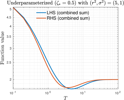
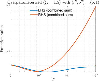
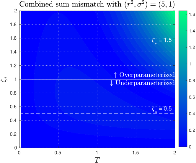
S.11.1.2 High signal-to-noise ratio

Figure S.14: Comparison of the LHS and RHS in (E.8) (combined sum) for the underparameterized (left) and overparameterized (right) regimes with high $\mathop{\mathrm{SNR}}=50$.

Figure S.15: Contour plot of the absolute value of the difference between LHS and RHS of (E.8) with $\mathop{\mathrm{SNR}}=50$. It is visually apparent that the mismatch gets worse with increasing signal energy, per our calculations in Section S.3.6.1.

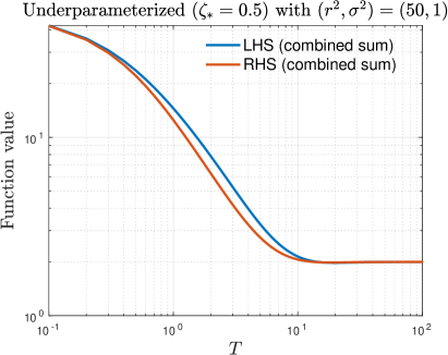
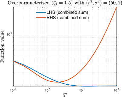
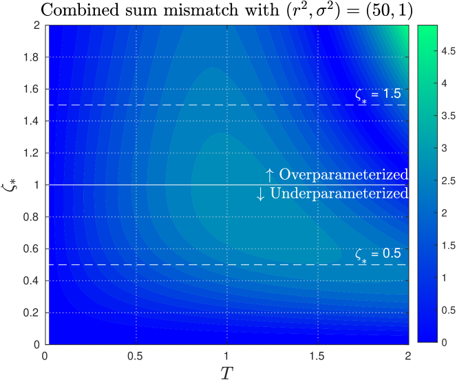
S.11.1.3 Low signal-to-noise ratio

Figure S.16: Comparison of the LHS and RHS in (E.8) (combined sum) for the underparameterized (left) and overparameterized (right) regimes with low $\mathop{\mathrm{SNR}}=0.2$.

Figure S.17: Contour plot of the absolute value of the difference between LHS and RHS of (E.8) with $\mathop{\mathrm{SNR}}=0.2$. We observe that the mismatch becomes worse with increasing noise energy. While the contours may look visually very similar, note that the range of values is higher in the right panel. The illustration is in line with our calculations in Section S.3.6.1.

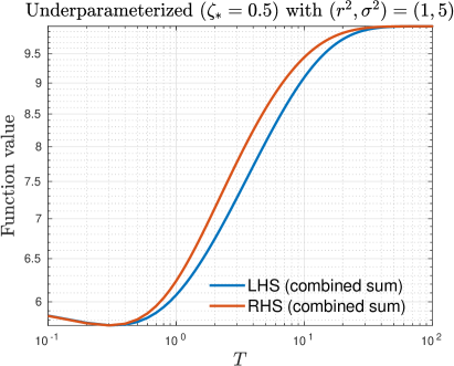
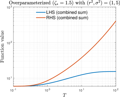
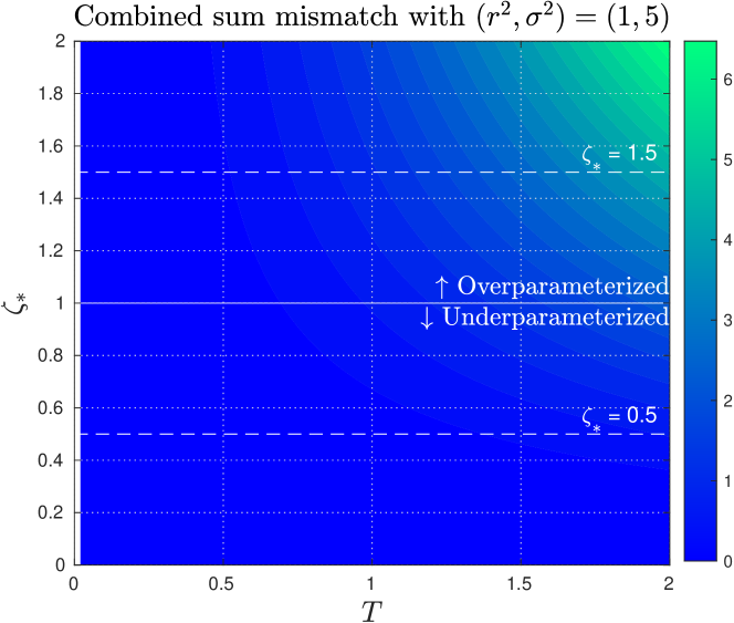
S.11.1.4 Very low signal-to-noise ratio

Figure S.18: Comparison of the LHS and RHS in (E.8) (combined sum) for the underparameterized (left) and overparameterized (right) regimes with very low $\mathop{\mathrm{SNR}}=0.02$.

Figure S.19: Contour plot of the absolute value of the difference between LHS and RHS of (E.8) with $\mathop{\mathrm{SNR}}=0.02$. We observe that the mismatch becomes worse with increasing noise energy. Although the contours may look visually very similar, note that the range of values is higher in the right panel. The illustration agrees with the calculations in Section S.3.6.1.

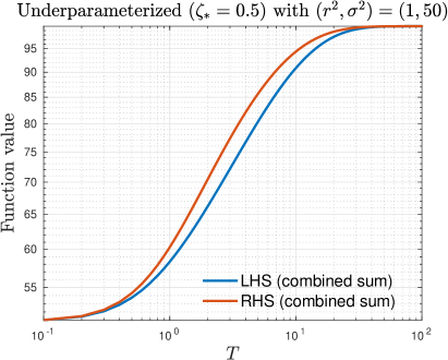
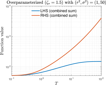
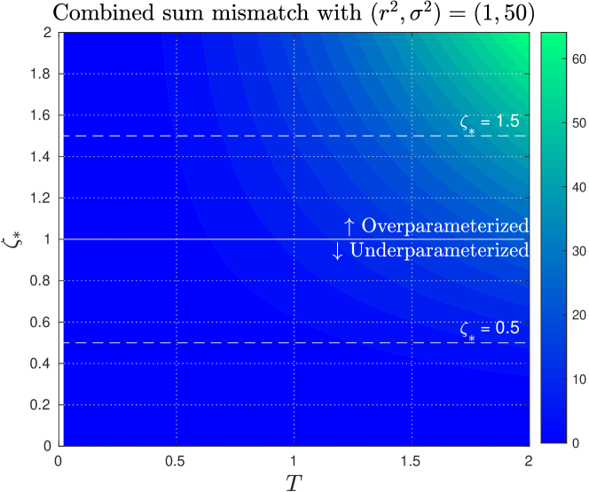
S.11.2 Additional setup details

S.11.2.1 Setup details for Figure 1

• Feature model: The feature vector $x_{i}\in\mathbb{R}^{p}$ is generated according to $x_{i}\sim\mathcal{N}(0,{I}_{p})$.

• Response model: Given feature vector $x_{i}$ for $i\in[n]$, the response variable $y_{i}\in\mathbb{R}$ is generated according to $y_{i}=x_{i}^{\top}\beta_{0}+\varepsilon_{i}$. where $\varepsilon_{i}\sim\mathcal{N}(0,\sigma^{2})$ with $\sigma^{2}=1$.

• Signal model: The signal vector is generated according to $\beta_{0}\sim\mathcal{N}(0,r^{2}p^{-1}I_{p})$ with $r^{2}=5$.

S.11.2.2 Setup details for Figure 3

• Feature model: The feature $x_{i}\in\mathbb{R}^{p}$ is generated according to

  $$\addcontentsline{lla}{section}{\numberline{\string\crtrefnumber{eq:feature_model}}{e}q:feature_{m}odel}x_{i}=\Sigma^{1/2}z_{i},$$ (E.65)

  where $z_{i}\in\mathbb{R}^{p}$ contains independently sampled entries from a common distribution, and $\Sigma\in\mathbb{R}^{p\times p}$ is a positive semidefinite feature covariance matrix. We use an autoregressive covariance structure such that $\Sigma_{ij}=\rho^{|i-j|}$ for all $i,j$ with parameter $\rho=0.25$.

• Response model: Given $x_{i}$, the response $y_{i}\in\mathbb{R}$ is generated according to

  $$\addcontentsline{lla}{section}{\numberline{\string\crtrefnumber{eq:response_model}}{e}q:response_{m}odel}y_{i}=\beta_{0}^{\top}x_{i}+\bigl{(}x_{i}^{\top}Ax_{i}-\operatorname{tr}[A\Sigma]\bigr{)}/p+\varepsilon_{i},$$ (E.66)

  where $\beta_{0}\in\mathbb{R}^{p}$ is a fixed signal vector, $A\in\mathbb{R}^{p\times p}$ is a fixed matrix, and $\varepsilon_{i}\in\mathbb{R}$ is a random noise variable. Note that we have subtracted the mean from the squared nonlinear component and scaled it to keep the variance of the nonlinear component at the same order as the noise variance (see Mei and Montanari (2022) for more details, for example). We again use Student’s $t$ distribution for the random noise component, which is again standardized so that the mean is zero and the variance is one.

• Signal model: We align the signal $\beta_{0}$ with the top eigenvector (corresponding to the largest eigenvalue) of the covariance matrix $\Sigma$. More precisely, suppose that $\Sigma=WRW^{\top}$ denotes the eigenvalue decomposition of the covariance matrix $\Sigma$, where $W\in\mathbb{R}^{p\times p}$ is an orthogonal matrix whose columns $w_{1},\dots,w_{p}$ are eigenvectors of $\Sigma$ and $R\in\mathbb{R}^{p\times p}$ is a diagonal matrix whose entries $r_{1}\geq\dots\geq r_{p}$ are eigenvalues of $\Sigma$ in descending order. We then let $\beta_{0}=cw_{1}$, where $c$ controls the effective signal energy. We refer to the value of $\beta_{0}^{\top}\Sigma\beta_{0}$ as the effective signal energy, which is set at $50$. It is worth noting that even though the regression function above does not satisfy the assumptions of Assumption C, it is easy to see that the function is approximately Lipschitz.

S.11.3 Additional illustration for predictive intervals based on LOOCV

See Figure S.20 for an additional illustration of the prediction intervals based on LOOCV where the optimal stopping occurs at an intermediate iteration. This is in contrast to Figure 3 where optimal stopping occurs at a far enough iteration, due to the “latent signal” structure. For Figure S.20, we use an isotropic setup under a linear model, similar to that of Figure 1.

For the sake of completeness, the details are described below:

• Feature model: The feature vector $x_{i}\in\mathbb{R}^{p}$ is generated according to $x_{i}\sim\mathcal{N}(0,{I}_{p})$.

• Response model: Given feature vector $x_{i}$ for $i\in[n]$, the response variable $y_{i}\in\mathbb{R}$ is generated according to $y_{i}=x_{i}^{\top}\beta_{0}+\varepsilon_{i}$, where $\varepsilon_{i}\sim\mathcal{N}(0,\sigma^{2})$ with $\sigma^{2}=1$.

• Signal model: The signal vector is generated according to $\beta_{0}\sim\mathcal{N}(0,r^{2}p^{-1}I_{p})$ with $r^{2}=5$.

Figure S.20: LOOCV provides prediction intervals with near-consistent coverage in finite samples across different nominal coverage levels. We consider an overparameterized regime, where the number of observations is $n=2500$ and the number of features is $p=5000$ (overparameterized). The non-intercept features are Gaussian with a $\rho$-autoregressive covariance $\Sigma$ (such that $\Sigma_{ij}=\rho^{|i-j|}$ for all $i,j$) with $\rho=0.25$. The response is generated from a linear model with a nonrandom signal vector $\beta_{0}$ that has unit Euclidean norm. We initialize the GD process randomly and employ a universal step size $\delta=0.01$. In the left panel, we plot the empirical coverage rates with various levels, and in the right panel, we plot the length of the prediction intervals. All simulation outcomes are based on one realization of $(X,y)$.

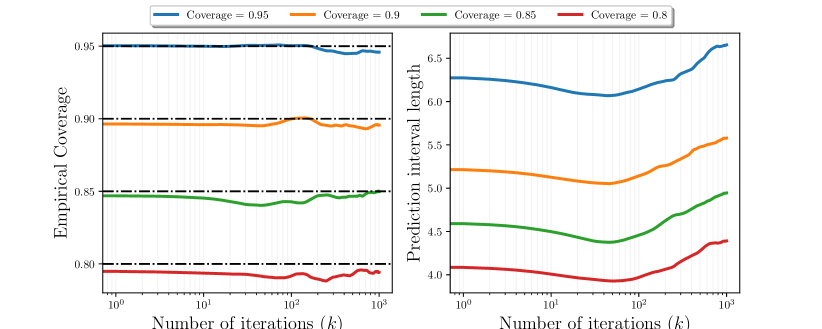
S.11.4 Additional illustrations for Section 4.2

S.11.4.1 Squared and absolute risk and LOOCV plug-in functionals

Figure S.21: LOOCV plug-in functionals are consistent for both squared and absolute error functionals. We use the same setup as shown in Figure 3 to demonstrate the consistency for the squared error and absolute error functionals.

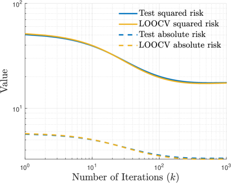
S.11.4.2 Ridgeline plot of test error and LOOCV error distributions

Figure S.22: Empirical distribution of LOOCV errors tracks the true test error distribution along the entire gradient descent path. We use the same setup as in Figure 3, but now visualize the evolution of the associated distribution in a single iteration-distribution ridgeline plot.

References

- Adlam and Pennington (2020) Ben Adlam and Jeffrey Pennington. Understanding double descent requires a fine-grained bias-variance decomposition. In Advances in Neural Information Processing Systems, 2020.
- Ali et al. (2019) Alnur Ali, J. Zico Kolter, and Ryan J. Tibshirani. A continuous-time view of early stopping for least squares regression. In International Conference on Artificial Intelligence and Statistics, 2019.
- Ali et al. (2020) Alnur Ali, Edgar Dobriban, and Ryan J. Tibshirani. The implicit regularization of stochastic gradient flow for least squares. In International Conference on Machine Learning, 2020.
- Allen (1974) David M. Allen. The relationship between variable selection and data augmentation and a method for prediction. Technometrics, 16(1):125–127, 1974.
- Arlot and Celisse (2010) Sylvain Arlot and Alain Celisse. A survey of cross-validation procedures for model selection. Statistics Surveys, 4:40–79, 2010.
- Auddy et al. (2023) Arnab Auddy, Haolin Zou, Kamiar Rahnama Rad, and Arian Maleki. Approximate leave-one-out cross validation for regression with regularizers. arXiv preprint arXiv:2310.17629, 2023.
- Austern and Zhou (2020) Morgane Austern and Wenda Zhou. Asymptotics of cross-validation. arXiv preprint arXiv:2001.11111, 2020.
- Avelin and Viitasaari (2022) Benny Avelin and Lauri Viitasaari. Concentration inequalities for leave-one-out cross validation. arXiv preprint arXiv:2211.02478, 2022.
- Bai and Silverstein (2010) Zhidong Bai and Jack W. Silverstein. Spectral Analysis of Large Dimensional Random Matrices. Springer, 2010.
- Bartlett et al. (2021) Peter L. Bartlett, Andrea Montanari, and Alexander Rakhlin. Deep learning: A statistical viewpoint. Acta Numerica, 30:87–201, 2021.
- Bauer et al. (2007) Frank Bauer, Sergei Pereverzev, and Lorenzo Rosasco. On regularization algorithms in learning theory. Journal of Complexity, 23(1):52–72, 2007.
- Bayati and Montanari (2011) Mohsen Bayati and Andrea Montanari. The dynamics of message passing on dense graphs, with applications to compressed sensing. IEEE Transactions on Information Theory, 57(2):764–785, 2011.
- Bayati et al. (2013) Mohsen Bayati, Murat A. Erdogdu, and Andrea Montanari. Estimating lasso risk and noise level. In Advances in Neural Information Processing Systems, 2013.
- Bayle et al. (2020) Pierre Bayle, Alexandre Bayle, Lucas Janson, and Lester Mackey. Cross-validation confidence intervals for test error. arXiv preprint arXiv:2007.12671, 2020.
- Belkin (2021) Misha Belkin. Fit without fear: Remarkable mathematical phenomena of deep learning through the prism of interpolation. Acta Numerica, 30:203–248, 2021.
- Bellec (2023) Pierre C. Bellec. Out-of-sample error estimate for robust M-estimators with convex penalty. Information and Inference, 12(4):2782–2817, 2023.
- Bellec and Shen (2022) Pierre C. Bellec and Yiwei Shen. Derivatives and residual distribution of regularized M-estimators with application to adaptive tuning. In Conference on Learning Theory, 2022.
- Berthier et al. (2023) Raphaël Berthier, Andrea Montanari, and Kangjie Zhou. Learning time-scales in two-layers neural networks. arXiv preprint arXiv:2303.00055, 2023.
- Bühlmann and Yu (2003) Peter Bühlmann and Bin Yu. Boosting with the loss: Regression and classification. Journal of the American Statistical Association, 98(462):324–339, 2003.
- Celentano et al. (2021) Michael Celentano, Chen Cheng, and Andrea Montanari. The high-dimensional asymptotics of first order methods with random data. arXiv preprint arXiv:2112.07572, 2021.
- Celisse and Guedj (2016) Alain Celisse and Benjamin Guedj. Stability revisited: New generalisation bounds for the leave-one-out. arXiv preprint arXiv:1608.06412, 2016.
- Chen et al. (2021) Hong-Bin Chen, Sinho Chewi, and Jonathan Niles-Weed. Dimension-free log-Sobolev inequalities for mixture distributions. Journal of Functional Analysis, 281(11):109236, 2021.
- Craven and Wahba (1979) Peter Craven and Grace Wahba. Estimating the correct degree of smoothing by the method of generalized cross-validation. Numerische Mathematik, 31:377–403, 1979.
- Dobriban and Wager (2018) Edgar Dobriban and Stefan Wager. High-dimensional asymptotics of prediction: Ridge regression and classification. Annals of Statistics, 46(1):247–279, 2018.
- Du et al. (2023) Jin-Hong Du, Pratik Patil, and Arun Kumar Kuchibhotla. Subsample ridge ensembles: Equivalences and generalized cross-validation. In International Conference on Machine Learning, 2023.
- Erdos and Yau (2017) László Erdos and Horng-Tzer Yau. A Dynamical Approach to Random Matrix Theory. Courant Lecture Notes in Mathematics, 2017.
- Geisser (1975) Seymour Geisser. The predictive sample reuse method with applications. Journal of the American Statistical Association, 70(350):320–328, 1975.
- Golub et al. (1979) Gene H. Golub, Michael Heath, and Grace Wahba. Generalized cross-validation as a method for choosing a good ridge parameter. Technometrics, 21(2):215–223, 1979.
- Gozlan (2009) Nathael Gozlan. A characterization of dimension free concentration in terms of transportation inequalities. Annals of Probability, 37(6):2480–2498, 2009.
- Gunasekar et al. (2018a) Suriya Gunasekar, Jason Lee, Daniel Soudry, and Nathan Srebro. Characterizing implicit bias in terms of optimization geometry. In International Conference on Machine Learning, 2018a.
- Gunasekar et al. (2018b) Suriya Gunasekar, Jason D. Lee, Daniel Soudry, and Nati Srebro. Implicit bias of gradient descent on linear convolutional networks. In Advances in Neural Information Processing Systems, 2018b.
- Han and Xu (2023) Qiyang Han and Xiaocong Xu. The distribution of ridgeless least squares interpolators. arXiv preprint arXiv:2307.02044, 2023.
- Hastie (2020) Trevor Hastie. Ridge regularization: An essential concept in data science. Technometrics, 62(4):426–433, 2020.
- Hastie et al. (2009) Trevor Hastie, Robert Tibshirani, and Jerome H. Friedman. The Elements of Statistical Learning: Data Mining, Inference, and Prediction. Springer, 2009. Second edition.
- Hastie et al. (2022) Trevor Hastie, Andrea Montanari, Saharon Rosset, and Ryan J. Tibshirani. Surprises in high-dimensional ridgeless least squares interpolation. Annals of Statistics, 50(2):949–986, 2022.
- Jansen et al. (1997) Maarten Jansen, Maurits Malfait, and Adhemar Bultheel. Generalized cross validation for wavelet thresholding. Signal Processing, 56(1):33–44, 1997.
- Ji and Telgarsky (2019) Ziwei Ji and Matus Telgarsky. The implicit bias of gradient descent on nonseparable data. In Conference on Learning Theory, 2019.
- Kale et al. (2011) Satyen Kale, Ravi Kumar, and Sergei Vassilvitskii. Cross-validation and mean-square stability. In Proceedings of the Second Symposium on Innovations in Computer Science, 2011.
- Kobak et al. (2020) Dmitry Kobak, Jonathan Lomond, and Benoit Sanchez. The optimal ridge penalty for real-world high-dimensional data can be zero or negative due to the implicit ridge regularization. Journal of Machine Learning Research, 21(169):1–16, 2020.
- Koepf (1998) Wolfram Koepf. Hypergeometric summation. Vieweg, Braunschweig/Wiesbaden, 5(6), 1998.
- Krantz and Parks (2002) Steven G. Krantz and Harold R. Parks. A Primer of Real Analytic Functions. Springer, 2002.
- Kumar et al. (2013) Ravi Kumar, Daniel Lokshtanov, Sergei Vassilvitskii, and Andrea Vattani. Near-optimal bounds for cross-validation via loss stability. In International Conference on Machine Learning, 2013.
- Landweber (1951) Louis Landweber. An iteration formula for Fredholm integral equations of the first kind. American Journal of Mathematics, 73(3):615–624, 1951.
- Lei (2020) Jing Lei. Cross-validation with confidence. Journal of the American Statistical Association, 115(532):1978–1997, 2020.
- Li (1985) Ker-Chau Li. From Stein’s unbiased risk estimates to the method of generalized cross validation. Annals of Statistics, 13(4):1352–1377, 1985.
- Li (1986) Ker-Chau Li. Asymptotic optimality of and generalized cross-validation in ridge regression with application to spline smoothing. Annals of Statistics, 14(3):1101–1112, 1986.
- Li (1987) Ker-Chau Li. Asymptotic optimality for , , cross-validation and generalized cross-validation: Discrete index set. Annals of Statistics, 15(3):958–975, 1987.
- Luo et al. (2023) Yuetian Luo, Zhimei Ren, and Rina Foygel Barber. Iterative approximate cross-validation. arXiv preprint arXiv:2303.02732, 2023.
- Mei and Montanari (2022) Song Mei and Andrea Montanari. The generalization error of random features regression: Precise asymptotics and the double descent curve. Communications on Pure and Applied Mathematics, 75(4):667–766, 2022.
- Miolane and Montanari (2021) Léo Miolane and Andrea Montanari. The distribution of the lasso: Uniform control over sparse balls and adaptive parameter tuning. Annals of Statistics, 49(4):2313–2335, 2021.
- Morgan and Bourlard (1989) Nelson Morgan and Hervé Bourlard. Generalization and parameter estimation in feedforward nets: Some experiments. In Advances in Neural Information Processing Systems, 1989.
- Nacson et al. (2019) Mor Shpigel Nacson, Nathan Srebro, and Daniel Soudry. Stochastic gradient descent on separable data: Exact convergence with a fixed learning rate. In International Conference on Artificial Intelligence and Statistics, 2019.
- Neu and Rosasco (2018) Gergely Neu and Lorenzo Rosasco. Iterate averaging as regularization for stochastic gradient descent. In Conference On Learning Theory, 2018.
- Patil and LeJeune (2024) Pratik Patil and Daniel LeJeune. Asymptotically free sketched ridge ensembles: Risks, cross-validation, and tuning. In International Conference on Learning Representations, 2024.
- Patil et al. (2021) Pratik Patil, Yuting Wei, Alessandro Rinaldo, and Ryan J. Tibshirani. Uniform consistency of cross-validation estimators for high-dimensional ridge regression. In International Conference on Artificial Intelligence and Statistics, 2021.
- Patil et al. (2022a) Pratik Patil, Arun Kumar Kuchibhotla, Yuting Wei, and Alessandro Rinaldo. Mitigating multiple descents: A model-agnostic framework for risk monotonization. arXiv preprint arXiv:2205.12937, 2022a.
- Patil et al. (2022b) Pratik Patil, Alessandro Rinaldo, and Ryan J. Tibshirani. Estimating functionals of the out-of-sample error distribution in high-dimensional ridge regression. In International Conference on Artificial Intelligence and Statistics, 2022b.
- Rad and Maleki (2020) Kamiar Rahnama Rad and Arian Maleki. A scalable estimate of the out-of-sample prediction error via approximate leave-one-out cross-validation. Journal of the Royal Statistical Society: Series B, 82(4):965–996, 2020.
- Rad et al. (2020) Kamiar Rahnama Rad, Wenda Zhou, and Arian Maleki. Error bounds in estimating the out-of-sample prediction error using leave-one-out cross validation in high-dimensions. In International Conference on Artificial Intelligence and Statistics, 2020.
- Raskutti et al. (2014) Garvesh Raskutti, Martin J. Wainwright, and Bin Yu. Early stopping and non-parametric regression: An optimal data-dependent stopping rule. The Journal of Machine Learning Research, 15(1):335–366, 2014.
- Richards et al. (2021) Dominic Richards, Jaouad Mourtada, and Lorenzo Rosasco. Asymptotics of ridge (less) regression under general source condition. In International Conference on Artificial Intelligence and Statistics, 2021.
- Rosset et al. (2004) Saharon Rosset, Ji Zhu, and Trevor Hastie. Boosting as a regularized path to a maximum margin classifier. Journal of Machine Learning Research, 5:941–973, 2004.
- Stephenson and Broderick (2020) William Stephenson and Tamara Broderick. Approximate cross-validation in high dimensions with guarantees. In International Conference on Artificial Intelligence and Statistics, 2020.
- Stone (1974) Mervyn Stone. Cross-validatory choice and assessment of statistical predictions. Journal of the Royal Statistical Society: Series B, 36(2):111–133, 1974.
- Stone (1977) Mervyn Stone. Asymptotics for and against cross-validation. Biometrika, 64(1):29–35, 1977.
- Strand (1974) Otto Neall Strand. Theory and methods related to the singular-function expansion and Landweber’s iteration for integral equations of the first kind. SIAM Journal on Numerical Analysis, 11(4):798–825, 1974.
- Suggala et al. (2018) Arun S. Suggala, Adarsh Prasad, and Pradeep Ravikumar. Connecting optimization and regularization paths. In Advances in Neural Information Processing Systems, 2018.
- Van Handel (2014) Ramon Van Handel. Probability in high dimension. Technical report, Princeton University, 2014.
- Vershynin (2010) Roman Vershynin. Introduction to the non-asymptotic analysis of random matrices. arXiv preprint arXiv:1011.3027, 2010.
- Vershynin (2018) Roman Vershynin. High-Dimensional Probability: An Introduction with Applications in Data Science. Cambridge University Press, 2018.
- Wang et al. (2018) Shuaiwen Wang, Wenda Zhou, Haihao Lu, Arian Maleki, and Vahab Mirrokni. Approximate leave-one-out for fast parameter tuning in high dimensions. In International Conference on Machine Learning, 2018.
- Wei et al. (2022) Alexander Wei, Wei Hu, and Jacob Steinhardt. More than a toy: Random matrix models predict how real-world neural representations generalize. In International Conference on Machine Learning, 2022.
- Wei et al. (2017) Yuting Wei, Fanny Yang, and Martin J. Wainwright. Early stopping for kernel boosting algorithms: A general analysis with localized complexities. In Advances in Neural Information Processing Systems, 2017.
- Wilson et al. (2020) Ashia Wilson, Maximilian Kasy, and Lester Mackey. Approximate cross-validation: Guarantees for model assessment and selection. In International Conference on Artificial Intelligence and Statistics, 2020.
- Wilson et al. (2017) Ashia C. Wilson, Rebecca Roelofs, Mitchell Stern, Nati Srebro, and Benjamin Recht. The marginal value of adaptive gradient methods in machine learning. In Advances in Neural Information Processing Systems, 2017.
- Wu and Xu (2020) Denny Wu and Ji Xu. On the optimal weighted regularization in overparameterized linear regression. In Advances in Neural Information Processing Systems, 2020.
- Yao et al. (2007) Yuan Yao, Lorenzo Rosasco, and Andrea Caponnetto. On early stopping in gradient descent learning. Constructive Approximation, 26(2):289–315, 2007.
- Zhang et al. (2017) Chiyuan Zhang, Samy Bengio, Moritz Hardt, Benjamin Recht, and Oriol Vinyals. Understanding deep learning requires rethinking generalization. In International Conference on Learning Representations, 2017.
- Zhang and Yu (2005) Tong Zhang and Bin Yu. Boosting with early stopping: Convergence and consistency. Annals of Statistics, 33(4):1538–1579, 2005.
- Zhang and Yang (2015) Yongli Zhang and Yuhong Yang. Cross-validation for selecting a model selection procedure. Journal of Econometrics, 187(1):95–112, 2015.