Rate-Optimal Rank Aggregation with Private Pairwise Rankings

Shirong Xu Statistics and Data Science, University of California, Los Angeles. Email: shirongxu56@ucla.edu    Will Wei Sun Daniels School of Business, Purdue University. Email:sun244@purdue.edu    Guang Cheng Statistics and Data Science, University of California, Los Angeles. Email: guangcheng@ucla.edu
Abstract

In various real-world scenarios like recommender systems and political surveys, pairwise rankings are commonly collected and utilized for rank aggregation to obtain an overall ranking of items. However, preference rankings can reveal individuals’ personal preferences, underscoring the need to protect them before releasing for downstream analysis. In this paper, we address the challenge of preserving privacy while ensuring the utility of rank aggregation based on pairwise rankings generated from the Bradley-Terry-Luce (BTL) model. Using the randomized response mechanism to perturb raw pairwise rankings is a common privacy protection strategy used in practice, but a critical challenge arises because the privatized rankings no longer adhere to the BTL model, resulting in significant bias in downstream rank aggregation tasks. Motivated from this, we propose a debiased randomized response mechanism to protect the raw pairwise rankings, ensuring consistent estimation of true preferences and rankings in downstream rank aggregation. Theoretically, we offer insights into the relationship between overall privacy guarantees and estimation errors from private ranking data, and establish minimax rates for estimation errors. This enables the determination of optimal privacy guarantees that balance consistency in rank aggregation with robust privacy protection. We also investigate convergence rates of expected ranking errors for partial and full ranking recovery, quantifying how privacy protection influences the specification of top-K𝐾K item sets and complete rankings. Our findings are validated through extensive simulations and a real application.

Keywords: Bradley-Terry-Luce Model, Differential Privacy, Minimax Optimality, Statistical Learning Theory, Ranking Data

1 Introduction

Ranking data frequently emerges in various scenarios, notably in recommender systems (Karatzoglou et al.,, 2013; Kalloori et al.,, 2018; Oliveira et al.,, 2020), political surveys (Ackerman et al.,, 2013; Nielson,, 2017; McCarthy and Santucci,, 2021), and search engines (Dwork et al.,, 2001; Liu et al.,, 2007). Among ranking data, pairwise ranking stands out as a particular form that finds applications in collecting customer preferences and political investigations. Particularly, Kalloori et al., (2018) developed a mobile app to collect users’ pairwise comparisons in preference for ranking items, while Ackerman et al., (2013) investigated the problem of collecting voters’ pairwise comparisons to determine the committee members. The collected individual noisy rankings can be used for various rank aggregation analyses, such as estimating the true underlying ranking (Negahban et al.,, 2016), specifying top-K𝐾K objects (Chen and Suh,, 2015; Shah and Wainwright,, 2018; Chen et al.,, 2022), and inferring relative ranking of two objects (Liu et al.,, 2023).

In recent years, there has been a growing concern about the privacy of personal data (Dwork,, 2006; Dwork and Roth,, 2014; Bi and Shen,, 2023; Shen et al.,, 2023), prompting numerous countries to respond by enacting specific regulations. One notable example is the General Data Protection Regulation (GDPR)111https://gdpr-info.eu/ in the European Union. The GDPR is designed to empower individuals with control over their personal data and mandates stringent data protection practices for businesses. Additionally, Canada has implemented the Personal Information Protection and Electronic Documents Act (PIPEDA)222https://www.priv.gc.ca/en/privacy-topics/privacy-laws-in-canada/ as a federal law governing the collection, use, and disclosure of personal data within the private sectors. These regulatory measures aim to address the evolving challenges associated with the protection of individuals’ private information. As a distinctive form of data, ranking data also inherently carries sensitivity as it has the potential to reveal personal preferences (Ichihashi,, 2020) or political inclinations (Lee,, 2015). Particularly, political views and voting behavior are considered sensitive personal data according to GDPR. Protecting ranking data not only ensures regulatory compliance but also encourages data sharing without privacy concerns, minimizing potential misreporting due to privacy worries. Effectively protecting ranking data poses a significant challenge as it involves preserving users’ privacy while maintaining the utility of privatized data for downstream rank aggregation analysis.

Consider a scenario wherein a third party aims to collect pairwise rankings via a sequence of pairwise comparison questions through some online platforms such as survey websites (Carlson and Montgomery,, 2017) or mobile apps (Kalloori et al.,, 2018). The objective of the third party is to conduct the rank aggregation that integrates rankings from various users into a unified ranking that accurately reflects the collective preferences of the group. Therefore, the objective of the online platforms is to protect the privacy of the submitted pairwise rankings, while maintaining the utility of ranking data for the downstream rank aggregation task. In this context, a natural challenge for the online platform is understanding the fundamental limit in the privacy-utility tradeoff in rank aggregation and addressing the question of how strong privacy protection can be enforced on individuals’ rankings given a specific number of respondents and items for comparison. See Figure 1 for an illustration.

Refer to caption
Figure 1: Utility-Preserving Private Pairwise Ranking Mechanism.

To model pairwise rankings, a common practice is to employ the Bradley-Terry-Luce (BTL) model (Bradley and Terry,, 1952; Luce,, 2012), which finds diverse applications spanning from sports tournaments (Xia et al.,, 2020; Karlé and Tyagi,, 2023) to human feedback for large language models (Zhu et al.,, 2023). In the BTL model, let 𝜽=(θ1,,θm)superscript𝜽superscriptsubscript𝜃1superscriptsubscript𝜃𝑚\bm{\theta}^{*}=(\theta_{1}^{*},\ldots,\theta_{m}^{*}) denote the preference vector of a set of items Ω={1,,m}Ω1𝑚\Omega=\{1,\ldots,m\}, where θi>θjsuperscriptsubscript𝜃𝑖superscriptsubscript𝜃𝑗\theta_{i}^{*}>\theta_{j}^{*} indicates that item i𝑖i is more preferred than item j𝑗j at the population level. The estimation of 𝜽superscript𝜽\bm{\theta}^{*} based on raw pairwise rankings has received recent attentions (Negahban et al.,, 2016; Chen et al.,, 2019; Liu et al.,, 2023). Nevertheless, protecting privacy of collected rankings in our framework inevitably distorts the raw distributions of rankings, rendering existing methods inapplicable.

In practical scenarios, a widely employed method for protecting ranking data is the randomized response (RR) mechanism (Warner,, 1965), wherein binary comparisons are flipped with a predetermined probability. Nonetheless, merely disclosing the private ranking data using the classic RR mechanism is inadequate. This is due to the fact that the privatized rankings no longer conform to the BTL model, leading to notable biases in subsequent rank aggregation tasks. To address this challenge, in this paper we introduce a debiased randomized response mechanism aimed at achieving both differential privacy (DP; Dwork, 2006) and preserving utility in subsequent rank aggregation tasks. The conceptual framework developed in this paper is visually represented in Figure 1. Initially, individuals’ rankings are collected through a ranking survey. These rankings then undergo permutation using a randomized mechanism and a subsequent debiasing step before being disclosed to a third party. The debiasing step is designed to align privatized rankings with the actual rankings in expectation. Following this, the debiased and private rankings are provided to the third party for preference ranking estimation via a regularized M-estimation procedure. Notably, our approach, which adapts to individuals’ diverse privacy preferences rather than enforcing a uniform standard, proves valuable for managing the widely acknowledged variability in privacy preferences among individuals (Okazaki et al.,, 2009; Costante et al.,, 2013).

Our paper makes the following three methodological and theoretical contributions:

  • 1

    Our first contribution is a debiased RR mechanism that ensures consistent rank aggregation estimation. This new method addresses the distortion in the raw distribution of output rankings caused by the classic RR mechanism, which deviates from the BTL model and leads to inconsistent estimation of 𝜽superscript𝜽\bm{\theta}^{*}. The debiasing step aims to align the expected values of privatized rankings with those of the actual rankings, enabling the direct application of existing estimation methods for the BTL model. Consequently, our privatized rankings ensure privacy protection while maintaining utility.

  • 2

    Secondly, we study the asymptotic behavior of estimation errors measured via 𝜽^𝜽2subscriptnorm^𝜽superscript𝜽2\|\widehat{\bm{\theta}}-\bm{\theta}^{*}\|_{2} and 𝜽^𝜽subscriptnorm^𝜽superscript𝜽\|\widehat{\bm{\theta}}-\bm{\theta}^{*}\|_{\infty} to evaluate the utility of the resulting estimator 𝜽^^𝜽\widehat{\bm{\theta}} based on private pairwise rankings. The main technical challenge in this context lies in precisely assessing how diverse privacy guarantees affect 𝜽^𝜽2subscriptnorm^𝜽superscript𝜽2\|\widehat{\bm{\theta}}-\bm{\theta}^{*}\|_{2} and 𝜽^𝜽subscriptnorm^𝜽superscript𝜽\|\widehat{\bm{\theta}}-\bm{\theta}^{*}\|_{\infty} due to their varying impact on information loss in the raw rankings. We analyze the influence of overall privacy on 𝜽^𝜽2subscriptnorm^𝜽superscript𝜽2\|\widehat{\bm{\theta}}-\bm{\theta}^{*}\|_{2} through a detailed examination of variance amplification in debiased rankings. Subsequently, leveraging the global optimality of 𝜽^^𝜽\widehat{\bm{\theta}}, we derive the convergence rate of 𝜽^𝜽subscriptnorm^𝜽superscript𝜽\|\widehat{\bm{\theta}}-\bm{\theta}^{*}\|_{\infty} based on that of 𝜽^𝜽2subscriptnorm^𝜽superscript𝜽2\|\widehat{\bm{\theta}}-\bm{\theta}^{*}\|_{2}. Moreover, we establish the minimax rate of the estimation errors based on the private rankings, demonstrating that the proposed estimator is minimax-optimal, up to a logarithmic term. Our theoretical results shed light on the fundamental limit of the privacy-utility tradeoff, allowing for the development of an optimal adaptive privacy scheme with respect to m𝑚m and L𝐿L, where m𝑚m and L𝐿L represent the numbers of items and users, respectively.

  • 3

    Another key issue in rank aggregation involves determining the minimum sample size necessary to accurately recover the true ranking of items. To address this issue, we establish the convergence rates of expected ranking errors in both top-K𝐾K recovery and full ranking recovery scenarios. Our theoretical findings unveil the sample complexity required to ensure consistent ranking recovery under diverse personalized privacy guarantees. Additionally, we validate our theoretical results through comprehensive simulations and analysis of a real-life dataset.

1.1 Related Work

There are two closely related lines of work, including the application of differential privacy on ranking data and the privacy-utility tradeoff in statistical estimation problems. Next we provide an overview of relevant studies and discuss their distinctions from our own work.

Differential Privacy on Ranking Data. Shang et al., (2014) proposed to utilize the Gaussian noise to contaminate the histogram of collected rankings for rank aggregation, while Hay et al., (2017); Alabi et al., (2022) employed the Laplace and Gaussian mechanisms to perturb pairwise comparisons. Yan et al., (2020) considered the rank aggregation based on rankings privatized via the randomized response mechanism or the Laplace mechanism. Jeong et al., (2022) studied the probability of recovering the individual ranking based on the privatized data and the level of privacy guarantee under different noise-additive mechanisms. The existing literature primarily focuses on rank aggregation within a non-parametric framework, leaving the fundamental limit in the privacy-utility tradeoff of rank aggregation tasks under the BTL model with privacy constraints unexplored. In our problem, while the classic RR mechanism has been shown to be more effective than noise-additive mechanisms, it inherently causes a shift in the underlying distribution of pairwise comparisons, resulting in significant biases in subsequent rank aggregation tasks. Moreover, the incorporation of user-level privacy in differentially private rank aggregation tasks has been neglected. To bridge these gaps, we approach the rank aggregation task through statistical estimation under the BTL model, aiming to offer an optimal solution for online platforms to reconcile the utility of ranking data for third parties with the diverse privacy preferences of users.

Fundamental Privacy-Utility Tradeoff. Another relevant line of research delves into understanding the privacy-utility tradeoff in estimation based on privatized data. Duchi et al., (2018) derived minimax bounds for several canonical families of problems under privacy constraints, including mean estimation, median estimation, generalized linear models, and non-parametric density estimation. Their theoretical results shed light on the statistical cost of privacy and characterize the fundamental limit in the statistical utility that a privacy-preserving mechanism can achieve. Wang and Xu, (2019) studied the sparse linear regression problem under the privacy protection of responses and established the convergence rate and minimax lower bound of estimation. Cai et al., (2021) established minimax lower bounds for private mean estimation and linear regression problems. Xu et al., (2023) considered the binary classification where responses are locally protected via the RR mechanism, quantifying the impact of privacy guarantees on the estimation of the optimal classifier. Chhor and Sentenac, (2023) quantified the impact of differential privacy on the estimation of a discrete distribution. In contrast to previous studies, our focus is on the fundamental limit of statistical estimation within the rank aggregation problem, providing both an upper bound and a minimax lower bound to accurately assess the impact of privacy within the pairwise ranking data framework. Additionally, we consider the privatization of ranking data based on users’ privacy preferences, aiming to quantify the overall impact of privacy guarantees on the rank aggregation task and provide insights into achievable privacy levels.

1.2 Paper Organization

After introducing necessary notations in Section 1.3, we introduce the background information on ranking data and the BTL model in Section 2. In Section 3, we explore the privacy protection aspects of the randomized response mechanism, highlighting the impracticality of the classic RR mechanism. We then introduce a debiased RR mechanism to address this limitation. Section 4 develops a regularized M-estimator for estimating the true preference parameter of the BTL model, demonstrating the statistical consistency of the resulting estimator in terms of parameter estimation, top-K𝐾K ranking recovery, and full ranking recovery. To support our theoretical findings, Section 5 includes comprehensive simulations and a real-data application. All proofs are deferred to the supplementary file.

1.3 Notation

For a positive integer n𝑛n, denote [n]={1,,n}delimited-[]𝑛1𝑛[n]=\{1,...,n\} to be the n𝑛n-set. Given two numbers a𝑎a and b𝑏b, we use ab=max{a,b}𝑎𝑏𝑎𝑏a\vee b=\max\{a,b\} and ab=min{a,b}𝑎𝑏𝑎𝑏a\wedge b=\min\{a,b\}. For a set S𝑆S, we let |S|𝑆|S| denote its cardinality. For two positive sequences {fn}n=1superscriptsubscriptsubscript𝑓𝑛𝑛1\{f_{n}\}_{n=1}^{\infty} and {gn}n=1superscriptsubscriptsubscript𝑔𝑛𝑛1\{g_{n}\}_{n=1}^{\infty}, we denote that fn=O(gn)subscript𝑓𝑛𝑂subscript𝑔𝑛f_{n}=O(g_{n}) or fngnless-than-or-similar-tosubscript𝑓𝑛subscript𝑔𝑛f_{n}\lesssim g_{n} if lim supn|fn|/gn<+subscriptlimit-supremum𝑛subscript𝑓𝑛subscript𝑔𝑛\limsup_{n\rightarrow\infty}|f_{n}|/g_{n}<+\infty. We let fngnasymptotically-equalssubscript𝑓𝑛subscript𝑔𝑛f_{n}\asymp g_{n} if fn=O(gn)subscript𝑓𝑛𝑂subscript𝑔𝑛f_{n}=O(g_{n}) and gn=O(fn)subscript𝑔𝑛𝑂subscript𝑓𝑛g_{n}=O(f_{n}). For a random variable Xnsubscript𝑋𝑛X_{n} and a sequence {an}n=1superscriptsubscriptsubscript𝑎𝑛𝑛1\{a_{n}\}_{n=1}^{\infty}, we denote that Xn=op(an)subscript𝑋𝑛subscript𝑜𝑝subscript𝑎𝑛X_{n}=o_{p}(a_{n}) is Xn/ansubscript𝑋𝑛subscript𝑎𝑛X_{n}/a_{n} converges to zero in probability and Xn=Op(an)subscript𝑋𝑛subscript𝑂𝑝subscript𝑎𝑛X_{n}=O_{p}(a_{n}) if Xn/ansubscript𝑋𝑛subscript𝑎𝑛X_{n}/a_{n} is stochastically bounded. Let I()𝐼I(\cdot) be the indicator function and I(A)=1𝐼𝐴1I(A)=1 if A𝐴A holds true and 0 otherwise. For a vector 𝒙𝒙\bm{x}, we let 𝒙2subscriptnorm𝒙2\|\bm{x}\|_{2} denote its l2subscript𝑙2l_{2}-norm and 𝒙subscriptnorm𝒙\|\bm{x}\|_{\infty} denote its lsubscript𝑙l_{\infty}-norm.

2 Preliminaries on BTL Model

In the realm of ranking data, users engage in comparing a set of items based on users’ relative preferences. In practical scenarios, ranking data typically manifests in two forms, contingent on the method of data collection. Primarily, rankings can be derived through pairwise comparisons between items (Kalloori et al.,, 2018), or by assigning ordinal ranks to the items (Hajek et al.,, 2014; Szörényi et al.,, 2015). This paper predominantly delves into the context of pairwise rankings, a scenario frequently encountered in political investigations (Ackerman et al.,, 2013), recommender systems (Kalloori et al.,, 2018), and the collection of human feedback for large language models (Zhu et al.,, 2023).

Let Ω={1,,m}Ω1𝑚\Omega=\{1,\ldots,m\} denote a set of m𝑚m items. In ranking data, a true preference vector exists, denoted as 𝜽=(θ1,,θm)Tsuperscript𝜽superscriptsuperscriptsubscript𝜃1superscriptsubscript𝜃𝑚𝑇\bm{\theta}^{*}=(\theta_{1}^{*},\ldots,\theta_{m}^{*})^{T}. Here θi>θjsuperscriptsubscript𝜃𝑖superscriptsubscript𝜃𝑗\theta_{i}^{*}>\theta_{j}^{*} signifies that item i𝑖i is ranked higher (preferred) than item j𝑗j in terms of the ground truth. Pairwise rankings among ΩΩ\Omega can be represented as a set of pairwise comparisons denoted by {𝒚(l)}l=1Lsuperscriptsubscriptsuperscript𝒚𝑙𝑙1𝐿\{\bm{y}^{(l)}\}_{l=1}^{L}, where 𝒚(l)superscript𝒚𝑙\bm{y}^{(l)} represents the set of pairwise comparisons by l𝑙l-th user and can be represented by m(m1)/2𝑚𝑚12m(m-1)/2 binary values:

𝒚(l)=(yij(l))i<j{0,1}m(m1)/2,superscript𝒚𝑙subscriptsuperscriptsubscript𝑦𝑖𝑗𝑙𝑖𝑗superscript01𝑚𝑚12\displaystyle\bm{y}^{(l)}=\left(y_{ij}^{(l)}\right)_{i<j}\in\{0,1\}^{m(m-1)/2},

where yij(l)=1superscriptsubscript𝑦𝑖𝑗𝑙1y_{ij}^{(l)}=1 indicates that item i𝑖i is observed to be preferred over item j𝑗j by the l𝑙l-th user.

In practice, 𝜽superscript𝜽\bm{\theta}^{*} is not observable, but instead noisy pairwise rankings can be collected from users. To model pairwise rankings, it is a common practice to employ BTL model (Bradley and Terry,, 1952; Luce,, 2012), which is one of the most widely used parametric models for pairwise rankings (Chen and Suh,, 2015; Chen et al.,, 2019, 2022). Specifically, it assumes that

yij(l)={1 with probability eθieθi+eθj,0 otherwise, for l=1,,L.formulae-sequencesuperscriptsubscript𝑦𝑖𝑗𝑙cases1 with probability superscript𝑒superscriptsubscript𝜃𝑖superscript𝑒superscriptsubscript𝜃𝑖superscript𝑒superscriptsubscript𝜃𝑗otherwise0 otherwiseotherwise for 𝑙1𝐿\displaystyle y_{ij}^{(l)}=\begin{cases}1\mbox{ with probability }\frac{e^{\theta_{i}^{*}}}{e^{\theta_{i}^{*}}+e^{\theta_{j}^{*}}},\\ 0\mbox{ otherwise},\end{cases}\mbox{ for }l=1,\ldots,L.

In BTL model, yij(l)superscriptsubscript𝑦𝑖𝑗𝑙y_{ij}^{(l)}’s are independent for all i<j𝑖𝑗i<j and l[L]𝑙delimited-[]𝐿l\in[L] given 𝜽superscript𝜽\bm{\theta}^{*} (Chen et al.,, 2019; Liu et al.,, 2023). It is worth noting that BTL model is invariant to adding 𝜽superscript𝜽\bm{\theta}^{*} by a constant c𝑐c. In other words, 𝜽superscript𝜽\bm{\theta}^{*} and 𝜽+c𝟏msuperscript𝜽𝑐subscript1𝑚\bm{\theta}^{*}+c\bm{1}_{m} are equivalent for any constant c𝑐c. Therefore, to tackle the issue of identifiability of 𝜽superscript𝜽\bm{\theta}^{*}, it is standard to impose an additional constraint on 𝜽superscript𝜽\bm{\theta}^{*} as l=1mθl=0superscriptsubscript𝑙1𝑚superscriptsubscript𝜃𝑙0\sum_{l=1}^{m}\theta_{l}^{*}=0 as in Gao et al., (2023) and Liu et al., (2023).

3 Differentially Private Pairwise Rankings

In this section, we first discuss a classic randomized response mechanism for protecting privacy in pairwise ranking data. We elucidate why this conventional approach proves impractical for our problem. Then, we present our debiased randomized response mechanism.

3.1 Infeasibility of Classic RR Mechanism

To ensure the privacy of these pairwise comparisons, a common method used in practice is the randomized response mechanism (Warner,, 1965; Arachchige et al.,, 2019; Li et al.,, 2023), which flips a binary value with a predetermined probability. In particular, we denote the randomized response (RR) mechanism with a flipping probability of p𝑝p as 𝒜psubscript𝒜𝑝\mathcal{A}_{p}. For a pairwise comparison yij(l)superscriptsubscript𝑦𝑖𝑗𝑙y_{ij}^{(l)}, a privacy-preserving ranking y~ij(l)superscriptsubscript~𝑦𝑖𝑗𝑙\widetilde{y}_{ij}^{(l)} is generated as

y~ij(l)=𝒜p(yij(l))={yij(l), with probability 1p,1yij(l), with probability p,superscriptsubscript~𝑦𝑖𝑗𝑙subscript𝒜𝑝superscriptsubscript𝑦𝑖𝑗𝑙casessuperscriptsubscript𝑦𝑖𝑗𝑙 with probability 1𝑝1superscriptsubscript𝑦𝑖𝑗𝑙 with probability 𝑝\displaystyle\widetilde{y}_{ij}^{(l)}=\mathcal{A}_{p}\left(y_{ij}^{(l)}\right)=\begin{cases}y_{ij}^{(l)},&\mbox{ with probability }1-p,\\ 1-y_{ij}^{(l)},&\mbox{ with probability }p,\end{cases}

where p𝑝p is the probability of flipping the observed value. The randomized response outputs the true value with probability 1p1𝑝1-p and the opposite value with probability p𝑝p.

The privacy guarantee of the RR mechanism can be characterized under the local differential privacy (LDP; Wang et al., 2017), which becomes popular in privacy protection and has now been applied in various real scenarios, including Google Chrome browser (Erlingsson et al.,, 2014) and macOS (Tang et al.,, 2017). The primary advantage of LDP lies in its capability to enable privacy protection mechanisms to be implemented at the users’ end, accommodating diverse privacy preferences. For instance, in the recommender system discussed in Kalloori et al., (2018), pairwise preferences can be protected based on individual users’ privacy preferences before being transmitted to a central server for learning purposes. The formal definition of ϵitalic-ϵ\epsilon-LDP is given as follows.

Definition 1.

(ϵitalic-ϵ\epsilon-local differential privacy) For any ϵ>0italic-ϵ0\epsilon>0, a randomized mechanism 𝒜𝒜\mathcal{A} is ϵitalic-ϵ\epsilon-local differentially private if for any different input y𝑦y and ysuperscript𝑦y^{\prime}

maxy~log|(𝒜(y)=y~)(𝒜(y)=y~)|ϵ,subscript~𝑦𝒜𝑦~𝑦𝒜superscript𝑦~𝑦italic-ϵ\displaystyle\max_{\widetilde{y}}\log\Big{|}\frac{\mathbb{P}(\mathcal{A}(y)=\widetilde{y})}{\mathbb{P}(\mathcal{A}(y^{\prime})=\widetilde{y})}\Big{|}\leq\epsilon,

where the probability is taken with respect to the randomness of 𝒜𝒜\mathcal{A}.

As discussed in Wasserman and Zhou, (2010), local differential privacy can be conceptually understood in terms of disclosure risk associated with the true values of individual data points. Considering an observed value denoted as y~~𝑦\widetilde{y}, the goal is to make it challenging to distinguish two hypotheses regarding the actual value: ysuperscript𝑦y^{\prime} versus y𝑦y. The difficulty of achieving this distinction is controlled by the privacy parameter ϵitalic-ϵ\epsilon.

The RR mechanism 𝒜psubscript𝒜𝑝\mathcal{A}_{p} satisfies ϵitalic-ϵ\epsilon-LDP when p=1/(1+exp(ϵ))𝑝11italic-ϵp=1/(1+\exp(\epsilon)) (Yang et al.,, 2020). Denote that pϵ=1/(1+exp(ϵ))subscript𝑝italic-ϵ11italic-ϵp_{\epsilon}=1/(1+\exp(\epsilon)), then 𝒜pϵsubscript𝒜subscript𝑝italic-ϵ\mathcal{A}_{p_{\epsilon}} ensures ϵitalic-ϵ\epsilon-LDP for an observed pairwise comparison. It is worth noting that pϵ<1/2subscript𝑝italic-ϵ12p_{\epsilon}<1/2 for any ϵ>0italic-ϵ0\epsilon>0, indicating that the flipping probability of pairwise comparisons is always smaller than 1/2121/2. The privacy protection of pairwise rankings through the RR mechanism can be characterized by the disclosure risk. Suppose that yij(l)=1subscriptsuperscript𝑦𝑙𝑖𝑗1y^{(l)}_{ij}=1, and then the probabilities of observing y~ij(l)=1superscriptsubscript~𝑦𝑖𝑗𝑙1\widetilde{y}_{ij}^{(l)}=1 and y~ij(l)=0superscriptsubscript~𝑦𝑖𝑗𝑙0\widetilde{y}_{ij}^{(l)}=0 are eϵ/(1+eϵ)superscript𝑒italic-ϵ1superscript𝑒italic-ϵe^{\epsilon}/(1+e^{\epsilon}) and 1/(1+eϵ)11superscript𝑒italic-ϵ1/(1+e^{\epsilon}), respectively. This implies that the third party can have the knowledge of user l𝑙l preferring item i𝑖i over item j𝑗j with probability eϵ/(1+eϵ)superscript𝑒italic-ϵ1superscript𝑒italic-ϵe^{\epsilon}/(1+e^{\epsilon}).

As shown in Figure 1, once pairwise rankings undergo privatization, the privatized rankings are released to a third party for downstream ranking aggregation analysis. Hence it is important to maintain the utility of the downstream analysis while protecting the raw ranking data. However, while it provides privacy protection, the classic RR mechanism alters the distribution of raw pairwise rankings as shown in the following lemma.

Lemma 1.

Suppose Yijsubscript𝑌𝑖𝑗Y_{ij} follows the BTL model with parameters θisuperscriptsubscript𝜃𝑖\theta_{i}^{*} and θjsuperscriptsubscript𝜃𝑗\theta_{j}^{*}. For any ϵ>0italic-ϵ0\epsilon>0, Y~ijsubscript~𝑌𝑖𝑗\widetilde{Y}_{ij} based on the RR mechanism 𝒜pϵsubscript𝒜subscript𝑝italic-ϵ\mathcal{A}_{p_{\epsilon}} follows the distribution as

Y~ij={1 with probability 12+eθieθjeθi+eθj(12pϵ),0 otherwise.subscript~𝑌𝑖𝑗cases1 with probability 12superscript𝑒superscriptsubscript𝜃𝑖superscript𝑒superscriptsubscript𝜃𝑗superscript𝑒superscriptsubscript𝜃𝑖superscript𝑒superscriptsubscript𝜃𝑗12subscript𝑝italic-ϵotherwise0 otherwiseotherwise\displaystyle\widetilde{Y}_{ij}=\begin{cases}1\mbox{ with probability }\frac{1}{2}+\frac{e^{\theta_{i}^{*}}-e^{\theta_{j}^{*}}}{e^{\theta_{i}^{*}}+e^{\theta_{j}^{*}}}(\frac{1}{2}-p_{\epsilon}),\\ 0\mbox{ otherwise}.\end{cases}

Hence Y~ijsubscript~𝑌𝑖𝑗\widetilde{Y}_{ij} no longer follows the BTL model.

Lemma 1 demonstrates that Y~ijsubscript~𝑌𝑖𝑗\widetilde{Y}_{ij} follows the Bernoulli distribution with a parameter of 12+eθieθjeθi+eθj(12pϵ)12superscript𝑒superscriptsubscript𝜃𝑖superscript𝑒superscriptsubscript𝜃𝑗superscript𝑒superscriptsubscript𝜃𝑖superscript𝑒superscriptsubscript𝜃𝑗12subscript𝑝italic-ϵ\frac{1}{2}+\frac{e^{\theta_{i}^{*}}-e^{\theta_{j}^{*}}}{e^{\theta_{i}^{*}}+e^{\theta_{j}^{*}}}(\frac{1}{2}-p_{\epsilon}). As stronger privacy guarantee is imposed on Yijsubscript𝑌𝑖𝑗Y_{ij} (i.e., as ϵ0italic-ϵ0\epsilon\rightarrow 0), the resulting pairwise comparison Y~ijsubscript~𝑌𝑖𝑗\widetilde{Y}_{ij} becomes less informative. This is because the RR mechanism implicitly injects noise into pairwise comparisons, shrinking the probability of Y~ij=1subscript~𝑌𝑖𝑗1\widetilde{Y}_{ij}=1 towards 1/2121/2. Since Y~ijsubscript~𝑌𝑖𝑗\widetilde{Y}_{ij} no longer follows BTL model, existing methods used for estimation in BTL model may fail in accurately estimating the true parameters based on privatized rankings. Therefore, as an online platform, releasing Y~ijsubscript~𝑌𝑖𝑗\widetilde{Y}_{ij} directly to the third party will lead to inaccurate estimation of the true preference vector 𝜽superscript𝜽\bm{\theta}^{*}. To highlight this point, we provide an example in the following.

Example 1.

Consider 𝛉=(θ1,θ2,θ3)superscript𝛉superscriptsubscript𝜃1superscriptsubscript𝜃2superscriptsubscript𝜃3\bm{\theta}^{*}=(\theta_{1}^{*},\theta_{2}^{*},\theta_{3}^{*}) satisfying θ2θ1=θ3θ2=log(2)superscriptsubscript𝜃2superscriptsubscript𝜃1superscriptsubscript𝜃3superscriptsubscript𝜃22\theta_{2}^{*}-\theta_{1}^{*}=\theta_{3}^{*}-\theta_{2}^{*}=\log(2) and pϵ=1/3subscript𝑝italic-ϵ13p_{\epsilon}=1/3. It can be verified that Y~12subscript~𝑌12\widetilde{Y}_{12} and Y~23subscript~𝑌23\widetilde{Y}_{23} follow the same Bernoulli distribution with parameter 5/9595/9, while Y~13subscript~𝑌13\widetilde{Y}_{13} follows the Bernoulli distribution with parameter 3/5353/5. If Y~ijsubscript~𝑌𝑖𝑗\widetilde{Y}_{ij}’s can be modeled under the BTL model, there should exists 𝛉3superscript𝛉superscript3\bm{\theta}^{\prime}\in\mathbb{R}^{3} such that 5/9=A1/(A1+1)59subscript𝐴1subscript𝐴115/9=A_{1}/(A_{1}+1) and 3/5=A2/(A2+1)35subscript𝐴2subscript𝐴213/5=A_{2}/(A_{2}+1), where A1=eθ1θ2subscript𝐴1superscript𝑒superscriptsubscript𝜃1superscriptsubscript𝜃2A_{1}=e^{\theta_{1}^{\prime}-\theta_{2}^{\prime}} and A2=eθ1θ3subscript𝐴2superscript𝑒superscriptsubscript𝜃1superscriptsubscript𝜃3A_{2}=e^{\theta_{1}^{\prime}-\theta_{3}^{\prime}}. However, there is no solution satisfying both equations.

Example 1 demonstrates the impracticality of sharing privatized pairwise rankings with a third party, who may misinterpret them as being generated from the BTL model. This highlights that classic RR-based privatized rankings cannot be faithfully represented by the BTL model. Hence, simply releasing the privatized ranking set from RR mechanism could lead to significant errors in downstream rank aggregation analysis.

3.2 Debiased RR Mechanism

To address the issues in the classic RR mechanism, we propose a debiased RR mechanism to protect the pairwise ranking data while preserving the utility of downstream rank aggregation. Specifically, after obtaining the privacy-preserving pairwise rankings {𝒚~(l)}l=1Lsuperscriptsubscriptsuperscript~𝒚𝑙𝑙1𝐿\{\widetilde{\bm{y}}^{(l)}\}_{l=1}^{L} output by the classic RR mechanism, given by y~ij(l)=𝒜pϵl(yij(l))superscriptsubscript~𝑦𝑖𝑗𝑙subscript𝒜subscript𝑝subscriptitalic-ϵ𝑙superscriptsubscript𝑦𝑖𝑗𝑙\widetilde{y}_{ij}^{(l)}=\mathcal{A}_{p_{\epsilon_{l}}}(y_{ij}^{(l)}), where ϵlsubscriptitalic-ϵ𝑙\epsilon_{l} denotes the privacy preference of user l𝑙l, in the second stage, we introduce an additional debiasing procedure:

zij(l)=(eϵl+1)y~ij(l)1eϵl1 for i<j and l[L].superscriptsubscript𝑧𝑖𝑗𝑙superscript𝑒subscriptitalic-ϵ𝑙1superscriptsubscript~𝑦𝑖𝑗𝑙1superscript𝑒subscriptitalic-ϵ𝑙1 for 𝑖𝑗 and 𝑙delimited-[]𝐿\displaystyle z_{ij}^{(l)}=\frac{(e^{\epsilon_{l}}+1)\widetilde{y}_{ij}^{(l)}-1}{e^{\epsilon_{l}}-1}\mbox{ for }i<j\mbox{ and }l\in[L]. (1)

The debiasing procedure in (1) enables us to derive an unbiased estimator for 𝔼(yij(l))𝔼superscriptsubscript𝑦𝑖𝑗𝑙\mathbb{E}(y_{ij}^{(l)}). Note that zij(l)superscriptsubscript𝑧𝑖𝑗𝑙z_{ij}^{(l)} is subject to two sources of randomness: the RR mechanism and Yijsubscript𝑌𝑖𝑗Y_{ij}.

Lemma 2.

For any ij𝑖𝑗i\neq j and l[L]𝑙delimited-[]𝐿l\in[L], the expectation and variance of zij(l)superscriptsubscript𝑧𝑖𝑗𝑙z_{ij}^{(l)} are given as

𝔼(zij(l))=eθieθi+eθj and Var(zij(l))=(eϵl+1eϵl1)2(14(1/2pϵl)2(eθieθjeθi+eθj)2).𝔼superscriptsubscript𝑧𝑖𝑗𝑙superscript𝑒superscriptsubscript𝜃𝑖superscript𝑒superscriptsubscript𝜃𝑖superscript𝑒superscriptsubscript𝜃𝑗 and Varsuperscriptsubscript𝑧𝑖𝑗𝑙superscriptsuperscript𝑒subscriptitalic-ϵ𝑙1superscript𝑒subscriptitalic-ϵ𝑙1214superscript12subscript𝑝subscriptitalic-ϵ𝑙2superscriptsuperscript𝑒superscriptsubscript𝜃𝑖superscript𝑒superscriptsubscript𝜃𝑗superscript𝑒superscriptsubscript𝜃𝑖superscript𝑒superscriptsubscript𝜃𝑗2\displaystyle\mathbb{E}\left(z_{ij}^{(l)}\right)=\frac{e^{\theta_{i}^{*}}}{e^{\theta_{i}^{*}}+e^{\theta_{j}^{*}}}\mbox{ and }\mathrm{Var}\left(z_{ij}^{(l)}\right)=\left(\frac{e^{\epsilon_{l}}+1}{e^{\epsilon_{l}}-1}\right)^{2}\left(\frac{1}{4}-(1/2-p_{\epsilon_{l}})^{2}\Big{(}\frac{e^{\theta_{i}^{*}}-e^{\theta_{j}^{*}}}{e^{\theta_{i}^{*}}+e^{\theta_{j}^{*}}}\Big{)}^{2}\right).

Lemma 2 explicates the mean and variance of zij(l)superscriptsubscript𝑧𝑖𝑗𝑙z_{ij}^{(l)} for any ij𝑖𝑗i\neq j and l[L]𝑙delimited-[]𝐿l\in[L]. Notably, it is important to highlight that zij(l)superscriptsubscript𝑧𝑖𝑗𝑙z_{ij}^{(l)} and yij(l)superscriptsubscript𝑦𝑖𝑗𝑙y_{ij}^{(l)} share the same mean but differ in their variance. Specifically, the variance of zij(l)superscriptsubscript𝑧𝑖𝑗𝑙z_{ij}^{(l)} is amplified by the privacy guarantee ϵlsubscriptitalic-ϵ𝑙\epsilon_{l}. Consequently, as the privacy parameter ϵlsubscriptitalic-ϵ𝑙\epsilon_{l} tends towards zero (stronger privacy protection), the variance of zij(l)superscriptsubscript𝑧𝑖𝑗𝑙z_{ij}^{(l)} also increases to infinity at the order O(ϵl2)𝑂superscriptsubscriptitalic-ϵ𝑙2O(\epsilon_{l}^{-2}), which can be directly observed using the fact that ex1xsuperscript𝑒𝑥1𝑥e^{x}-1\approx x when x𝑥x is small. This result is of particular significance as it helps quantify the impact of ϵitalic-ϵ\epsilon on the estimation of 𝜽superscript𝜽\bm{\theta}^{*}.

Through the debiasing procedure, privatized rankings 𝒁(l)=(zij(l))i<jsuperscript𝒁𝑙subscriptsuperscriptsubscript𝑧𝑖𝑗𝑙𝑖𝑗\bm{Z}^{(l)}=(z_{ij}^{(l)})_{i<j} can be directly released to the third party for the estimation of 𝜽superscript𝜽\bm{\theta}^{*} and other ranking aggregation analysis.

4 Differentially Private Rank Aggregation

In this section, we develop theoretical results regarding the consistency in rank aggregation based on the debiased private pairwise rankings. In Section 4.1, we develop a differentially private estimator based on {𝒁(l)}l=1Lsuperscriptsubscriptsuperscript𝒁𝑙𝑙1𝐿\{\bm{Z}^{(l)}\}_{l=1}^{L} and evaluate the overall influence of varying personalized privacy preferences on the convergence rates of the estimation errors, measured in terms of both the l2subscript𝑙2l_{2}-norm and the lsubscript𝑙l_{\infty}-norm. Furthermore, we establish the minimax rates for the estimation errors, enabling us to derive the optimal privacy guarantee while maintaining the consistency of the rank aggregation task. We then proceed to analyze the convergence rates of the expected top-K𝐾K ranking error and the full ranking error between the resultant ranking derived by the proposed estimator and the true ranking in Sections 4.2 and 4.3, respectively, where we also quantify the impact of privacy on the convergence rates of these metrics.

4.1 Parameter Estimation

We first present theoretical results pertaining to the estimation of the true preference vector 𝜽superscript𝜽\bm{\theta}^{*} based on private pairwise rankings. In the literature on the BTL model, when there is no privacy guarantee (ϵ=)italic-ϵ(\epsilon=\infty), the estimation of 𝜽superscript𝜽\bm{\theta}^{*} is commonly implemented through regularized maximum likelihood estimation (MLE) (Chen et al.,, 2019) that minimizes

~λ(𝜽)=subscript~𝜆𝜽absent\displaystyle\widetilde{\mathcal{L}}_{\lambda}(\bm{\theta})= i<j{y¯ijlogeθieθi+eθj+(1y¯ij)logeθjeθi+eθj}+λ𝜽22,subscript𝑖𝑗subscript¯𝑦𝑖𝑗superscript𝑒subscript𝜃𝑖superscript𝑒subscript𝜃𝑖superscript𝑒subscript𝜃𝑗1subscript¯𝑦𝑖𝑗superscript𝑒subscript𝜃𝑗superscript𝑒subscript𝜃𝑖superscript𝑒subscript𝜃𝑗𝜆superscriptsubscriptnorm𝜽22\displaystyle-\sum_{i<j}\Big{\{}\overline{y}_{ij}\log\frac{e^{\theta_{i}}}{e^{\theta_{i}}+e^{\theta_{j}}}+(1-\overline{y}_{ij})\log\frac{e^{\theta_{j}}}{e^{\theta_{i}}+e^{\theta_{j}}}\Big{\}}+\lambda\|\bm{\theta}\|_{2}^{2}, (2)

where y¯ij=l=1Lyij(l)/Lsubscript¯𝑦𝑖𝑗superscriptsubscript𝑙1𝐿superscriptsubscript𝑦𝑖𝑗𝑙𝐿\overline{y}_{ij}=\sum_{l=1}^{L}y_{ij}^{(l)}/L. In our framework, the released debiased privatized rankings {𝒁(l)}l=1Lsuperscriptsubscriptsuperscript𝒁𝑙𝑙1𝐿\{\bm{Z}^{(l)}\}_{l=1}^{L} are used as surrogates for {𝒚(l)}l=1Lsuperscriptsubscriptsuperscript𝒚𝑙𝑙1𝐿\{\bm{y}^{(l)}\}_{l=1}^{L} by the third-party, then the optimization task becomes

λ(𝜽)=subscript𝜆𝜽absent\displaystyle\mathcal{L}_{\lambda}(\bm{\theta})= i<j{z¯ijlogeθieθi+eθj+(1z¯ij)logeθjeθi+eθj}+λ𝜽22subscript𝑖𝑗subscript¯𝑧𝑖𝑗superscript𝑒subscript𝜃𝑖superscript𝑒subscript𝜃𝑖superscript𝑒subscript𝜃𝑗1subscript¯𝑧𝑖𝑗superscript𝑒subscript𝜃𝑗superscript𝑒subscript𝜃𝑖superscript𝑒subscript𝜃𝑗𝜆superscriptsubscriptnorm𝜽22\displaystyle-\sum_{i<j}\Big{\{}\overline{z}_{ij}\log\frac{e^{\theta_{i}}}{e^{\theta_{i}}+e^{\theta_{j}}}+(1-\overline{z}_{ij})\log\frac{e^{\theta_{j}}}{e^{\theta_{i}}+e^{\theta_{j}}}\Big{\}}+\lambda\|\bm{\theta}\|_{2}^{2}
=\displaystyle= i<j{z¯ij(θjθi)+log(1+eθiθj)}+λ𝜽22,subscript𝑖𝑗subscript¯𝑧𝑖𝑗subscript𝜃𝑗subscript𝜃𝑖1superscript𝑒subscript𝜃𝑖subscript𝜃𝑗𝜆superscriptsubscriptnorm𝜽22\displaystyle\sum_{i<j}\Big{\{}\overline{z}_{ij}(\theta_{j}-\theta_{i})+\log(1+e^{\theta_{i}-\theta_{j}})\Big{\}}+\lambda\|\bm{\theta}\|_{2}^{2}, (3)

where z¯ij=l=1Lzij(l)/Lsubscript¯𝑧𝑖𝑗superscriptsubscript𝑙1𝐿superscriptsubscript𝑧𝑖𝑗𝑙𝐿\overline{z}_{ij}=\sum_{l=1}^{L}z_{ij}^{(l)}/L and λ>0𝜆0\lambda>0 is regularization parameter. As previously mentioned, the true preference parameter vector 𝜽superscript𝜽\bm{\theta}^{*} is non-unique, primarily because of its invariant optimality to constant shift. Here the regularization is used to ensure the uniqueness of the solution from minimizing λ(𝜽)subscript𝜆𝜽\mathcal{L}_{\lambda}(\bm{\theta}) (Chen et al.,, 2019; Liu et al.,, 2023). Here (4.1) is a convex optimization task, and hence the stationary point of applying gradient descent will give the optimal minimizer 𝜽^^𝜽\widehat{\bm{\theta}}.

Lemma 3.

For any λ>0𝜆0\lambda>0, 𝛉^^𝛉\widehat{\bm{\theta}} satisfies that 𝟏T𝛉^=0superscript1𝑇^𝛉0\bm{1}^{T}\widehat{\bm{\theta}}=0.

Lemma 3 demonstrates that the regularization term plays a vital role in ensuring the uniqueness of the solution to 𝓛𝝀(𝜽)subscript𝓛𝝀𝜽\bm{\mathcal{L}_{\lambda}(\bm{\theta})}, thereby ensuring alignment with the true preference parameter within the same constraint 𝟏T𝜽^=0superscript1𝑇^𝜽0\bm{1}^{T}\widehat{\bm{\theta}}=0.

We proceed to investigate a range of theoretical properties of 𝜽^^𝜽\widehat{\bm{\theta}} in order to understand the tradeoff between utility and privacy guarantees. Let κ=maxieθiminieθi𝜅subscript𝑖superscript𝑒superscriptsubscript𝜃𝑖subscript𝑖superscript𝑒superscriptsubscript𝜃𝑖\kappa=\frac{\max_{i}e^{\theta_{i}^{*}}}{\min_{i}e^{\theta_{i}^{*}}} be the condition number. Thus, |θiθj|logκsuperscriptsubscript𝜃𝑖superscriptsubscript𝜃𝑗𝜅|\theta_{i}^{*}-\theta_{j}^{*}|\leq\log\kappa for any i,j𝑖𝑗i,j, which further leads to that 𝜽<logκsubscriptnormsuperscript𝜽𝜅\|\bm{\theta}^{*}\|_{\infty}<\log\kappa and 𝜽2<mlogκsubscriptnormsuperscript𝜽2𝑚𝜅\|\bm{\theta}^{*}\|_{2}<\sqrt{m}\log\kappa. To establish the convergence of 𝜽^^𝜽\widehat{\bm{\theta}} to 𝜽superscript𝜽\bm{\theta}^{*}, we begin by examining the following quantity defined as:

eL(𝜽^,𝜽)=1m2Li<j,l𝔼(ij(𝜽^,𝒁(l))ij(𝜽,𝒁(l))),subscript𝑒𝐿^𝜽superscript𝜽1superscript𝑚2𝐿subscript𝑖𝑗𝑙𝔼subscript𝑖𝑗^𝜽superscript𝒁𝑙subscript𝑖𝑗superscript𝜽superscript𝒁𝑙\displaystyle e_{L}(\widehat{\bm{\theta}},\bm{\theta}^{*})=\frac{1}{m^{2}L}\sum_{i<j,l}\mathbb{E}\big{(}\mathcal{L}_{ij}(\widehat{\bm{\theta}},\bm{Z}^{(l)})-\mathcal{L}_{ij}(\bm{\theta}^{*},\bm{Z}^{(l)})\big{)}, (4)

where ij(𝜽,𝒁(l))=zij(l)(θjθi)+log(1+eθiθj)subscript𝑖𝑗𝜽superscript𝒁𝑙superscriptsubscript𝑧𝑖𝑗𝑙subscript𝜃𝑗subscript𝜃𝑖1superscript𝑒subscript𝜃𝑖subscript𝜃𝑗\mathcal{L}_{ij}(\bm{\theta},\bm{Z}^{(l)})=z_{ij}^{(l)}(\theta_{j}-\theta_{i})+\log(1+e^{\theta_{i}-\theta_{j}}), and 𝒁(l)=(zij(l))i<jsuperscript𝒁𝑙subscriptsuperscriptsubscript𝑧𝑖𝑗𝑙𝑖𝑗\bm{Z}^{(l)}=(z_{ij}^{(l)})_{i<j}. Here (4) quantifies the dissimilarity between 𝜽^^𝜽\widehat{\bm{\theta}} and 𝜽superscript𝜽\bm{\theta}^{*} in terms of the excess risk, which can be considered as the population-level analog of (4.1) with λ=0𝜆0\lambda=0. Subsequently, we present the following results concerning the convergence of eL(𝜽^,𝜽)subscript𝑒𝐿^𝜽superscript𝜽e_{L}(\widehat{\bm{\theta}},\bm{\theta}^{*}).

Theorem 1.

Let G(ϵ)=L1l=1L(eϵl+1eϵl1)2𝐺bold-ϵsuperscript𝐿1superscriptsubscript𝑙1𝐿superscriptsuperscript𝑒subscriptitalic-ϵ𝑙1superscript𝑒subscriptitalic-ϵ𝑙12G(\bm{\epsilon})=L^{-1}\sum_{l=1}^{L}\left(\frac{e^{\epsilon_{l}}+1}{e^{\epsilon_{l}}-1}\right)^{2} and H(ϵ)=maxl[L]eϵl+1eϵl1𝐻bold-ϵsubscript𝑙delimited-[]𝐿superscript𝑒subscriptitalic-ϵ𝑙1superscript𝑒subscriptitalic-ϵ𝑙1H(\bm{\epsilon})=\max_{l\in[L]}\frac{e^{\epsilon_{l}}+1}{e^{\epsilon_{l}}-1}. Choosing λmG(ϵ)log(mL)L𝛉22less-than-or-similar-to𝜆𝑚𝐺bold-ϵ𝑚𝐿𝐿superscriptsubscriptnormsuperscript𝛉22\lambda\lesssim\frac{mG(\bm{\epsilon})\log(mL)}{L\|\bm{\theta}^{*}\|_{2}^{2}} yields that for any δm,LκG(ϵ)log(mL)mLgreater-than-or-equivalent-tosubscript𝛿𝑚𝐿𝜅𝐺bold-ϵ𝑚𝐿𝑚𝐿\delta_{m,L}\gtrsim\kappa G(\bm{\epsilon})\frac{\log(mL)}{mL}, the following holds

(eL(𝜽^,𝜽)δm,L)exp(Cm2L(ρ(ϵ,κ))1δm,L),less-than-or-similar-tosubscript𝑒𝐿^𝜽superscript𝜽subscript𝛿𝑚𝐿𝐶superscript𝑚2𝐿superscript𝜌bold-italic-ϵ𝜅1subscript𝛿𝑚𝐿\displaystyle\mathbb{P}\left(e_{L}(\widehat{\bm{\theta}},\bm{\theta}^{*})\geq\delta_{m,L}\right)\lesssim\exp\left(-Cm^{2}L(\rho(\bm{\epsilon},\kappa))^{-1}\delta_{m,L}\right), (5)

for some positive constant C𝐶C, where ρ(ϵ,κ)=(1+κ)max{H(ϵ),G(ϵ)}𝜌bold-ϵ𝜅1𝜅𝐻bold-ϵ𝐺bold-ϵ\rho(\bm{\epsilon},\kappa)=(1+\kappa)\max\{H(\bm{\epsilon}),G(\bm{\epsilon})\}.

Theorem 1 establishes the convergence of 𝜽^^𝜽\widehat{\bm{\theta}} towards 𝜽superscript𝜽\bm{\theta}^{*} in terms of the excess risk, indicating that eL(𝜽^,𝜽)subscript𝑒𝐿^𝜽superscript𝜽e_{L}(\widehat{\bm{\theta}},\bm{\theta}^{*}) approaches zero at any order δm,Lsubscript𝛿𝑚𝐿\delta_{m,L} satisfying δm,L(1+κ)2G(ϵ)log(mL)mLgreater-than-or-equivalent-tosubscript𝛿𝑚𝐿superscript1𝜅2𝐺bold-italic-ϵ𝑚𝐿𝑚𝐿\delta_{m,L}\gtrsim(1+\kappa)^{2}G(\bm{\epsilon})\frac{\log(mL)}{mL}. Unlike existing results regarding consistent estimation of 𝜽superscript𝜽\bm{\theta}^{*} based on i.i.d. pairwise rankings by different users, a key difference of our estimator 𝜽^^𝜽\widehat{\bm{\theta}} is that the private and debiased pairwise rankings of users are not identically distributed due to varying privacy preferences. Therefore, it is necessary to quantify the impact of overall privacy on the debiased rankings, which is characterized by G(ϵ)𝐺bold-italic-ϵG(\bm{\epsilon}) in Theorem 1. Here G(ϵ)𝐺bold-italic-ϵG(\bm{\epsilon}) can be interpreted as the averaged privacy guarantee on rankings based on user preferences. The significance of Theorem 1 is two-fold. Firstly, it reveals that a more stringent privacy constraint imposed on rankings (i.e., a larger value of G(ϵ)𝐺bold-italic-ϵG(\bm{\epsilon})) results in a slower convergence of eL(𝜽^,𝜽)subscript𝑒𝐿^𝜽superscript𝜽e_{L}(\widehat{\bm{\theta}},\bm{\theta}^{*}). Secondly, Theorem 1 provides a foundation for quantifying the entrywise error of 𝜽^^𝜽\widehat{\bm{\theta}}, which paves the way for establishing the ranking errors in Sections 4.2 and 4.3.

Theorem 2.

Under the conditions of Theorem 1, we have the following two results concerning the convergence of 𝛉^^𝛉\widehat{\bm{\theta}} to 𝛉superscript𝛉\bm{\theta}^{*}:

  • (1)

    With probability at least 12exp(Cmlog(mL)min{G(ϵ)/H(ϵ),1})12𝐶𝑚𝑚𝐿𝐺bold-italic-ϵ𝐻bold-italic-ϵ11-2\exp\big{(}-Cm\log(mL)\min\{G(\bm{\epsilon})/H(\bm{\epsilon}),1\}\big{)},

    1m𝜽^𝜽2κG(ϵ)log(mL)mL.less-than-or-similar-to1𝑚subscriptnorm^𝜽superscript𝜽2𝜅𝐺bold-italic-ϵ𝑚𝐿𝑚𝐿\displaystyle\frac{1}{\sqrt{m}}\|\widehat{\bm{\theta}}-\bm{\theta}^{*}\|_{2}\lesssim\kappa\sqrt{\frac{G(\bm{\epsilon})\log(mL)}{mL}}. (6)
  • (2)

    With probability at least 12mL22exp(Cmlog(mL)min{G(ϵ)/H(ϵ),1})12𝑚superscript𝐿22𝐶𝑚𝑚𝐿𝐺bold-italic-ϵ𝐻bold-italic-ϵ11-\frac{2}{mL^{2}}-2\exp(-Cm\log(mL)\min\{G(\bm{\epsilon})/H(\bm{\epsilon}),1\}),

    𝜽^𝜽κ2G(ϵ)log(mL)mL.less-than-or-similar-tosubscriptnorm^𝜽superscript𝜽superscript𝜅2𝐺bold-italic-ϵ𝑚𝐿𝑚𝐿\displaystyle\|\widehat{\bm{\theta}}-\bm{\theta}^{*}\|_{\infty}\lesssim\kappa^{2}\sqrt{\frac{G(\bm{\epsilon})\log(mL)}{mL}}. (7)

The establishment of Theorem 2 is on top of Theorem 1. Specifically, we first establish the quantitative relation between eL(𝜽^,𝜽)subscript𝑒𝐿^𝜽superscript𝜽e_{L}(\widehat{\bm{\theta}},\bm{\theta}^{*}) and 𝜽^𝜽2subscriptnorm^𝜽superscript𝜽2\|\widehat{\bm{\theta}}-\bm{\theta}^{*}\|_{2}, which allows us to establish the convergence rate for 𝜽^𝜽2subscriptnorm^𝜽superscript𝜽2\|\widehat{\bm{\theta}}-\bm{\theta}^{*}\|_{2} as in (6). Furthermore, we establish an upper bound for the entry-wise error of 𝜽^^𝜽\widehat{\bm{\theta}} using 𝜽^𝜽2subscriptnorm^𝜽superscript𝜽2\|\widehat{\bm{\theta}}-\bm{\theta}^{*}\|_{2} and δm,Lsubscript𝛿𝑚𝐿\delta_{m,L} defined in Theorem 1, which then leads to the convergence rate of 𝜽^𝜽subscriptnorm^𝜽superscript𝜽\|\widehat{\bm{\theta}}-\bm{\theta}^{*}\|_{\infty} in (7). Theorem 2 provides theoretical results regarding the asymptotic behavior of the estimation errors of 𝜽^^𝜽\widehat{\bm{\theta}} concerning its convergence toward 𝜽superscript𝜽\bm{\theta}^{*}. This convergence is measured using the l2subscript𝑙2l_{2}-norm and lsubscript𝑙l_{\infty}-norm. It is clear that increasing the number of rankings (L𝐿L) or items (m𝑚m) results in a more accurate estimation of the true preference parameter vector 𝜽superscript𝜽\bm{\theta}^{*} for any fixed ϵbold-italic-ϵ\bm{\epsilon}. However, when privacy constraints are imposed on pairwise comparisons, the convergence rate of 𝜽^^𝜽\widehat{\bm{\theta}} is notably slowed by a multiplicative constant of G(ϵ)𝐺bold-italic-ϵ\sqrt{G(\bm{\epsilon})}. Here it is worth noting that G(ϵ)>H(ϵ)𝐺bold-italic-ϵ𝐻bold-italic-ϵG(\bm{\epsilon})>H(\bm{\epsilon}) when privacy concern of users are homogeneous, i.e., ϵl=ϵsubscriptitalic-ϵ𝑙italic-ϵ\epsilon_{l}=\epsilon for each l[L]𝑙delimited-[]𝐿l\in[L].

A particular theoretical insight from Theorems 1 and 2 offers a quantification of how the average privacy protection of users impacts the convergence of 𝜽^^𝜽\widehat{\bm{\theta}}. This result holds particular significance in understanding the fundamental limit of privacy protection that can be achieved while maintaining consistency of 𝜽^^𝜽\widehat{\bm{\theta}} in estimating 𝜽superscript𝜽\bm{\theta}^{*}. Notably, in the absence of privacy constraints (as ϵlsubscriptitalic-ϵ𝑙\epsilon_{l} approaches infinity), our results reduce to the existing non-private one, up to a logarithmic term (Chen and Suh,, 2015; Chen et al.,, 2019).

Corollary 1.

Suppose all users have identical privacy preferences, i.e., ϵl=ϵsubscriptitalic-ϵ𝑙italic-ϵ\epsilon_{l}=\epsilon for l[L]𝑙delimited-[]𝐿l\in[L]. Given that ϵlog(mL)mLgreater-than-or-equivalent-toitalic-ϵ𝑚𝐿𝑚𝐿\epsilon\gtrsim\frac{\log(mL)}{\sqrt{mL}}, we have 𝔼𝒟~(m12𝛉^𝛉2)=o(1)subscript𝔼~𝒟superscript𝑚12subscriptnorm^𝛉superscript𝛉2𝑜1\mathbb{E}_{\widetilde{\mathcal{D}}}\big{(}m^{-\frac{1}{2}}\|\widehat{\bm{\theta}}-\bm{\theta}^{*}\|_{2}\big{)}=o(1) and 𝔼𝒟~(𝛉^𝛉)=o(1)subscript𝔼~𝒟subscriptnorm^𝛉superscript𝛉𝑜1\mathbb{E}_{\widetilde{\mathcal{D}}}\big{(}\|\widehat{\bm{\theta}}-\bm{\theta}^{*}\|_{\infty}\big{)}=o(1).

Corollary 1 naturally follows from Theorem 1 by employing an adaptive approach for setting ϵitalic-ϵ\epsilon based on the values of L𝐿L and m𝑚m. This adaptive scheme signifies that as either the number of rankings or items increases, a higher level of privacy protection (smaller ϵitalic-ϵ\epsilon) can be achieved for each pairwise comparison, while maintaining the consistency in estimating 𝜽superscript𝜽\bm{\theta}^{*}.

To gain deeper insights into the limit of privacy protection, we establish the minimax rates of the estimation errors based on privatized pairwise rankings in Theorem 3.

Theorem 3 (Minimax Rate).

Let 𝒟~={𝐲~(l)}l=1L~𝒟superscriptsubscriptsuperscript~𝐲𝑙𝑙1𝐿\widetilde{\mathcal{D}}=\{\widetilde{\bm{y}}^{(l)}\}_{l=1}^{L} denote a set of privatized pairwise rankings. For any estimator 𝛉^^𝛉\widehat{\bm{\theta}} based on 𝒟~~𝒟\widetilde{\mathcal{D}}, we have

inf𝜽^sup𝜽Θ𝔼𝒟~[𝜽^𝜽]inf𝜽^sup𝜽Θ𝔼𝒟~[m12𝜽^𝜽2]1κml=1L(eϵl1eϵl+1)2subscriptinfimum^𝜽subscriptsupremumsuperscript𝜽Θsubscript𝔼~𝒟delimited-[]subscriptnorm^𝜽superscript𝜽subscriptinfimum^𝜽subscriptsupremumsuperscript𝜽Θsubscript𝔼~𝒟delimited-[]superscript𝑚12subscriptnorm^𝜽superscript𝜽2greater-than-or-equivalent-to1𝜅𝑚superscriptsubscript𝑙1𝐿superscriptsuperscript𝑒subscriptitalic-ϵ𝑙1superscript𝑒subscriptitalic-ϵ𝑙12\displaystyle\inf_{\widehat{\bm{\theta}}}\sup_{\bm{\theta}^{*}\in\Theta}\mathbb{E}_{\widetilde{\mathcal{D}}}\left[\|\widehat{\bm{\theta}}-\bm{\theta}^{*}\|_{\infty}\right]\geq\inf_{\widehat{\bm{\theta}}}\sup_{\bm{\theta}^{*}\in\Theta}\mathbb{E}_{\widetilde{\mathcal{D}}}\left[m^{-\frac{1}{2}}\|\widehat{\bm{\theta}}-\bm{\theta}^{*}\|_{2}\right]\gtrsim\frac{1}{\sqrt{\kappa m\sum_{l=1}^{L}\left(\frac{e^{\epsilon_{l}}-1}{e^{\epsilon_{l}}+1}\right)^{2}}} (8)

where the expectation is taken with respect to the randomness of raw rankings and the privacy mechanism.

Theorem 3 introduces the minimax rates of the estimation errors. It’s noteworthy that when ϵisubscriptitalic-ϵ𝑖\epsilon_{i} values are uniformly set to ϵitalic-ϵ\epsilon, the minimax rate simplifies to eϵ+1κmL(eϵ1)superscript𝑒italic-ϵ1𝜅𝑚𝐿superscript𝑒italic-ϵ1\frac{e^{\epsilon}+1}{\sqrt{\kappa mL}(e^{\epsilon}-1)}. This rate aligns with the upper bound on the convergence rate of 𝜽^^𝜽\widehat{\bm{\theta}} up to a logarithmic term, showing that the estimator 𝜽^^𝜽\widehat{\bm{\theta}} derived from the proposed debiased M-estimator is minimax optimal, achieving the best possible performance while allowing for a logarithmic term. This result showcases the efficiency and effectiveness of the proposed estimator 𝜽^^𝜽\widehat{\bm{\theta}} under privacy protection constraints. Additionally, a main characteristic of our minimax rate is considering varying privacy concerns among users, which remains largely unexplored in the current literature regarding estimation based on differentially private data.

Corollary 2.

Suppose that ϵi1mLasymptotically-equalssubscriptitalic-ϵ𝑖1𝑚𝐿\epsilon_{i}\asymp\frac{1}{\sqrt{mL}} for i[L]𝑖delimited-[]𝐿i\in[L], then it holds true that 𝔼𝒟~(m12𝛉^𝛉2)>csubscript𝔼~𝒟superscript𝑚12subscriptnorm^𝛉superscript𝛉2𝑐\mathbb{E}_{\widetilde{\mathcal{D}}}\big{(}m^{-\frac{1}{2}}\|\widehat{\bm{\theta}}-\bm{\theta}^{*}\|_{2}\big{)}>c and 𝔼𝒟~(𝛉^𝛉)>csubscript𝔼~𝒟subscriptnorm^𝛉superscript𝛉𝑐\mathbb{E}_{\widetilde{\mathcal{D}}}\big{(}\|\widehat{\bm{\theta}}-\bm{\theta}^{*}\|_{\infty}\big{)}>c for some positive constant c𝑐c.

Corollary 2 can be derived from Theorem 3 by selecting ϵlsubscriptitalic-ϵ𝑙\epsilon_{l} to be of the order 1mL1𝑚𝐿\frac{1}{\sqrt{mL}} for each user l𝑙l. Under this adaptive approach, achieving consistency in the estimation of 𝜽superscript𝜽\bm{\theta}^{*} is clearly unattainable. By merging Corollary 1 and 2, we observe that the order 1mL1𝑚𝐿\frac{1}{\sqrt{mL}} is a critical threshold influencing the convergence of 𝜽^^𝜽\widehat{\bm{\theta}}. This underscores that, under the adaptive privacy scheme for each pairwise ranking, the strongest privacy protection should be weaker than ϵ1mLasymptotically-equalsitalic-ϵ1𝑚𝐿\epsilon\asymp\frac{1}{\sqrt{mL}} in order to ensure the utility of rank aggregation task.

Table 1: The behavior of estimation errors under different schemes of adaptive privacy guarantee as m𝑚m or L𝐿L increases given that ϵl=ϵsubscriptitalic-ϵ𝑙italic-ϵ\epsilon_{l}=\epsilon.
ϵitalic-ϵ\epsilon 𝔼𝒟~(m12𝜽^𝜽2)subscript𝔼~𝒟superscript𝑚12subscriptnorm^𝜽superscript𝜽2\mathbb{E}_{\widetilde{\mathcal{D}}}\left(m^{-\frac{1}{2}}\|\widehat{\bm{\theta}}-\bm{\theta}^{*}\|_{2}\right) 𝔼𝒟~(𝜽^𝜽)subscript𝔼~𝒟subscriptnorm^𝜽superscript𝜽\mathbb{E}_{\widetilde{\mathcal{D}}}\left(\|\widehat{\bm{\theta}}-\bm{\theta}^{*}\|_{\infty}\right)
ϵ1log(mL)mLasymptotically-equalsitalic-ϵ1𝑚𝐿𝑚𝐿\epsilon\asymp\frac{1}{\log(mL)\sqrt{mL}} Increase Increase
ϵ1mLasymptotically-equalsitalic-ϵ1𝑚𝐿\epsilon\asymp\frac{1}{\sqrt{mL}} Remain Stable Remain Stable
ϵlog(mL)mLasymptotically-equalsitalic-ϵ𝑚𝐿𝑚𝐿\epsilon\asymp\frac{\log(mL)}{\sqrt{mL}} Decrease Decrease

4.2 Top-K𝐾K Ranking Recovery

In addition to the parameter estimation, another challenge in the domain of ranking is obtaining the list of top-K𝐾K items (Chen and Suh,, 2015; Suh et al.,, 2017). For example, in recommender systems, only products placed in the first few positions are readily accessible to customer, and hence recommender systems usually care about whether they place the K𝐾K most preferred items for each customer. This endeavor inherently revolves around distinguishing between the K𝐾K-th and (K+1)𝐾1(K+1)-th most preferred items. In this section, our focus is on establishing the convergence rate of the ranking error associated with 𝜽^^𝜽\widehat{\bm{\theta}} when selecting the top-K𝐾K items. In comparison to parameter estimation, achieving an accurate ranking order is a more manageable task, as obtaining the correct ordering of items does not necessarily imply consistency in parameter estimation.

Specifically, let θ(k)superscriptsubscript𝜃𝑘\theta_{(k)}^{*} represent the preference parameter of the k𝑘k-th largest preferred item. The difficulty of this challenge inherently hinges on the degree of separation between θ(k)superscriptsubscript𝜃𝑘\theta_{(k)}^{*} and θ(k+1)superscriptsubscript𝜃𝑘1\theta_{(k+1)}^{*}. In other words, when θ(k)θ(k+1)much-greater-thansuperscriptsubscript𝜃𝑘superscriptsubscript𝜃𝑘1\theta_{(k)}^{*}\gg\theta_{(k+1)}^{*}, the task of identifying the top-K𝐾K items becomes considerably easy. In the following Theorem, we shed light on the sample complexity required for recovering the exact top-K𝐾K identification.

Theorem 4 (Top-K𝐾K identification).

Using 𝛉^^𝛉\widehat{\bm{\theta}} obtained from the debiased regularized M-estimation under the conditions of Theorem 1, the set of top-K𝐾K items can be recovered exactly with probability at least 12mL2exp(Cmlog(mL)min{G(ϵ)/H(ϵ),1})12𝑚superscript𝐿2𝐶𝑚𝑚𝐿𝐺bold-ϵ𝐻bold-ϵ11-\frac{2}{mL^{2}}-\exp\left(-Cm\log(mL)\min\{G(\bm{\epsilon})/H(\bm{\epsilon}),1\}\right) if

m2L2G(ϵ)κ4mlog(mL)ΔK2,greater-than-or-equivalent-tosuperscript𝑚2𝐿2𝐺bold-italic-ϵsuperscript𝜅4𝑚𝑚𝐿superscriptsubscriptΔ𝐾2\displaystyle\frac{m^{2}L}{2}\gtrsim G(\bm{\epsilon})\frac{\kappa^{4}m\log(mL)}{\Delta_{K}^{2}},

where K=θ(K)θ(K+1)\bigtriangleup_{K}=\theta_{(K)}^{*}-\theta_{(K+1)}^{*} denotes the gap between the K𝐾K-th and the (K+1)𝐾1(K+1)-th largest preference parameters.

As demonstrated in Theorem 4, it is evident that the total number of pairwise comparisons m2L/2superscript𝑚2𝐿2m^{2}L/2 must exceed c1κ4G(ϵ)mlog(mL)K2subscript𝑐1superscript𝜅4𝐺bold-italic-ϵ𝑚𝑚𝐿superscriptsubscript𝐾2c_{1}\kappa^{4}G(\bm{\epsilon})\frac{m\log(mL)}{\bigtriangleup_{K}^{2}} to ensure the recovery of the top-K𝐾K list of items, where c1subscript𝑐1c_{1} is a sufficiently large constant. Here it is worth noting that the sample complexity is directly influenced by the privacy protection measured by G(ϵ)𝐺bold-italic-ϵG(\bm{\epsilon}). Consequently, stronger privacy necessitates a larger sample size to ensure the exact recovery of the top-K𝐾K item list.

Next, we aim to analyze the asymptotic behavior of the error about selecting the top-K𝐾K items. To this end, we define the function σ(𝜽)=(σ(θi))i[m]𝜎𝜽subscript𝜎subscript𝜃𝑖𝑖delimited-[]𝑚\sigma(\bm{\theta})=(\sigma(\theta_{i}))_{i\in[m]}, where σ(θi)𝜎subscript𝜃𝑖\sigma(\theta_{i}) represents the rank of θisubscript𝜃𝑖\theta_{i} within the values of 𝜽𝜽\bm{\theta}. To illustrate, if σ(θi)=k𝜎subscript𝜃𝑖𝑘\sigma(\theta_{i})=k, it signifies that item i𝑖i is the k𝑘k-th highest value among θisubscript𝜃𝑖\theta_{i}’s. Then we consider the normalized Hamming distance between 𝜽^^𝜽\widehat{\bm{\theta}} and 𝜽superscript𝜽\bm{\theta}^{*} (Shah and Wainwright,, 2018; Chen et al.,, 2022), which is defined as

HK(𝜽^,𝜽)=12K(i=1mI(σ(θ^i)>K,σ(θi)K)+i=1mI(σ(θ^i)K,σ(θi)>K)).subscript𝐻𝐾^𝜽superscript𝜽12𝐾superscriptsubscript𝑖1𝑚𝐼formulae-sequence𝜎subscript^𝜃𝑖𝐾𝜎superscriptsubscript𝜃𝑖𝐾superscriptsubscript𝑖1𝑚𝐼formulae-sequence𝜎subscript^𝜃𝑖𝐾𝜎superscriptsubscript𝜃𝑖𝐾\displaystyle H_{K}(\widehat{\bm{\theta}},\bm{\theta}^{*})=\frac{1}{2K}\left(\sum_{i=1}^{m}I\left(\sigma(\widehat{\theta}_{i})>K,\sigma(\theta_{i}^{*})\leq K\right)+\sum_{i=1}^{m}I\left(\sigma(\widehat{\theta}_{i})\leq K,\sigma(\theta_{i}^{*})>K\right)\right).

Here HK(𝜽^,𝜽)subscript𝐻𝐾^𝜽superscript𝜽H_{K}(\widehat{\bm{\theta}},\bm{\theta}^{*}) takes values in {0,1K,2K,,1}01𝐾2𝐾1\{0,\frac{1}{K},\frac{2}{K},\ldots,1\} and HK(𝜽^,𝜽)=0subscript𝐻𝐾^𝜽superscript𝜽0H_{K}(\widehat{\bm{\theta}},\bm{\theta}^{*})=0 only when {i[m]:σ(θ^i)K}={i[m]:σ(θi)K}conditional-set𝑖delimited-[]𝑚𝜎subscript^𝜃𝑖𝐾conditional-set𝑖delimited-[]𝑚𝜎superscriptsubscript𝜃𝑖𝐾\{i\in[m]:\sigma(\widehat{\theta}_{i})\leq K\}=\{i\in[m]:\sigma(\theta_{i}^{*})\leq K\}. It is worth noting that achieving a top-K𝐾K ranking error of zero does not necessitate the consistency of 𝜽^^𝜽\widehat{\bm{\theta}} but merely entails alignment between 𝜽^^𝜽\widehat{\bm{\theta}} and 𝜽superscript𝜽\bm{\theta}^{*} in ranking items. In the following lemma, we establish an upper bound for 𝔼(HK(𝜽^,𝜽))𝔼subscript𝐻𝐾^𝜽superscript𝜽\mathbb{E}\left(H_{K}(\widehat{\bm{\theta}},\bm{\theta}^{*})\right), building upon the probabilistic behavior of 𝜽^^𝜽\widehat{\bm{\theta}}.

Lemma 4.

For any 𝛉superscript𝛉\bm{\theta}^{*}, the following inequality holds for any estimator 𝛉^^𝛉\widehat{\bm{\theta}} and any K[m1]𝐾delimited-[]𝑚1K\in[m-1]:

𝔼(HK(𝜽^,𝜽))1K[i:σ(θi)K(θ^iθ(K)+θ(K+1)2)+i:σ(θi)>K(θ^iθ(K)+θ(K+1)2)].𝔼subscript𝐻𝐾^𝜽superscript𝜽1𝐾delimited-[]subscript:𝑖𝜎superscriptsubscript𝜃𝑖𝐾subscript^𝜃𝑖superscriptsubscript𝜃𝐾superscriptsubscript𝜃𝐾12subscript:𝑖𝜎superscriptsubscript𝜃𝑖𝐾subscript^𝜃𝑖superscriptsubscript𝜃𝐾superscriptsubscript𝜃𝐾12\displaystyle\mathbb{E}\big{(}H_{K}(\widehat{\bm{\theta}},\bm{\theta}^{*})\big{)}\leq\frac{1}{K}\left[\sum_{i:\sigma(\theta_{i}^{*})\leq K}\mathbb{P}\left(\widehat{\theta}_{i}\leq\frac{\theta_{(K)}^{*}+\theta_{(K+1)}^{*}}{2}\right)+\sum_{i:\sigma(\theta_{i}^{*})>K}\mathbb{P}\left(\widehat{\theta}_{i}\geq\frac{\theta_{(K)}^{*}+\theta_{(K+1)}^{*}}{2}\right)\right].

Lemma 4 offers a way to quantify the error associated with utilizing 𝜽^^𝜽\widehat{\bm{\theta}} for identifying the top-K𝐾K item set.

Theorem 5.

Assume that H(ϵ)mG(ϵ)less-than-or-similar-to𝐻bold-ϵ𝑚𝐺bold-ϵH(\bm{\epsilon})\lesssim mG(\bm{\epsilon}). Under the assumptions of Theorem 1 and Theorem 2, the top-K𝐾K ranking error of 𝛉^^𝛉\widehat{\bm{\theta}} satisfies

𝔼(HK(𝜽^,𝜽))exp(C0mLΔK2G(ϵ)κ4),less-than-or-similar-to𝔼subscript𝐻𝐾^𝜽superscript𝜽subscript𝐶0𝑚𝐿superscriptsubscriptΔ𝐾2𝐺bold-italic-ϵsuperscript𝜅4\displaystyle\mathbb{E}\left(H_{K}(\widehat{\bm{\theta}},\bm{\theta}^{*})\right)\lesssim\exp\left(-\frac{C_{0}mL\Delta_{K}^{2}}{G(\bm{\epsilon})\kappa^{4}}\right),

for some positive constants C0subscript𝐶0C_{0}.

Theorem 5 reveals that the expected ranking error exhibits exponential convergence under privacy constraints. Notably, an increase in the number of rankings or items augments the precision of identifying the top-K𝐾K item set for any fixed value of ϵbold-italic-ϵ\bm{\epsilon}. Furthermore, Theorem 5 delivers a similar insight into the influence of privacy guarantees. So long as G(ϵ)=O(mL/log(mL))𝐺bold-italic-ϵ𝑂𝑚𝐿𝑚𝐿G(\bm{\epsilon})=O(mL/\log(mL)), 𝔼(HK(𝜽^,𝜽))𝔼subscript𝐻𝐾^𝜽superscript𝜽\mathbb{E}\big{(}H_{K}(\widehat{\bm{\theta}},\bm{\theta}^{*})\big{)} will approach zero as either L𝐿L or m𝑚m grows.

4.3 Full Ranking Recovery

Acquiring a full ranking of items constitutes a fundamental challenge within the domains of ranking and preference modeling. Obtaining the full ranking of items based on user preferences is instrumental in enhancing the efficiency of a recommender system, enabling the system to place items according to the established preference order, thereby optimizing the user experience and enhancing business efficiency. Compared with the top-K𝐾K ranking recovery problem, the difficulty of obtaining the accurate full ranking hinges on the differences between θ(i)superscriptsubscript𝜃𝑖\theta_{(i)}^{*} and θ(i+1)superscriptsubscript𝜃𝑖1\theta_{(i+1)}^{*} for all i[m]𝑖delimited-[]𝑚i\in[m]. In this section, we delve into the theoretical aspects of the asymptotic behavior of full ranking error, with the aim of quantifying the impact of privacy guarantee on the error of recovering the full ranking. To this end, we consider the Kendall’s tau distance, as defined by

K(𝜽^,𝜽)=2m(m1)1i<jmI((σ(θ^i)σ(θ^j))(σ(θi)σ(θj))<0).𝐾^𝜽superscript𝜽2𝑚𝑚1subscript1𝑖𝑗𝑚𝐼𝜎subscript^𝜃𝑖𝜎subscript^𝜃𝑗𝜎superscriptsubscript𝜃𝑖𝜎superscriptsubscript𝜃𝑗0\displaystyle K(\widehat{\bm{\theta}},\bm{\theta}^{*})=\frac{2}{m(m-1)}\sum_{1\leq i<j\leq m}I\left(\big{(}\sigma(\widehat{\theta}_{i})-\sigma(\widehat{\theta}_{j})\big{)}\big{(}\sigma(\theta_{i}^{*})-\sigma(\theta_{j}^{*})\big{)}<0\right).

Here K(𝜽^,𝜽)𝐾^𝜽superscript𝜽K(\widehat{\bm{\theta}},\bm{\theta}^{*}) measures the percentage of pairs of items that are ranked inaccurately between the rankings induced from 𝜽^^𝜽\widehat{\bm{\theta}} and 𝜽superscript𝜽\bm{\theta}^{*}. Taking the expectation of K(𝜽^,𝜽)𝐾^𝜽superscript𝜽K(\widehat{\bm{\theta}},\bm{\theta}^{*}), we get

𝔼(K(𝜽^,𝜽))=2m(m1)(i,j):σ(θi)>σ(θj)(θ^i<θ^j).𝔼𝐾^𝜽superscript𝜽2𝑚𝑚1subscript:𝑖𝑗𝜎superscriptsubscript𝜃𝑖𝜎superscriptsubscript𝜃𝑗subscript^𝜃𝑖subscript^𝜃𝑗\displaystyle\mathbb{E}\left(K(\widehat{\bm{\theta}},\bm{\theta}^{*})\right)=\frac{2}{m(m-1)}\sum_{(i,j):\sigma(\theta_{i}^{*})>\sigma(\theta_{j}^{*})}\mathbb{P}\left(\widehat{\theta}_{i}<\widehat{\theta}_{j}\right). (9)

The relationship described in (9) reveals that the average full ranking error can be expressed equivalently as the average probability of incorrectly ranking two items. Consequently, it is adequate to focus on the right-hand side of (9) in order to establish the asymptotic behavior of 𝔼(K(𝜽^,𝜽))𝔼𝐾^𝜽superscript𝜽\mathbb{E}\left(K(\widehat{\bm{\theta}},\bm{\theta}^{*})\right).

Theorem 6.

Assume that H(ϵ)mG(ϵ)less-than-or-similar-to𝐻bold-ϵ𝑚𝐺bold-ϵH(\bm{\epsilon})\lesssim mG(\bm{\epsilon}). Under the assumptions of Theorem 1 and Theorem 2, the full ranking error of 𝛉^^𝛉\widehat{\bm{\theta}} satisfies

𝔼(K(𝜽^,𝜽))2m1i=1m1exp(C0mLΔi2G(ϵ)κ4),less-than-or-similar-to𝔼𝐾^𝜽superscript𝜽2𝑚1superscriptsubscript𝑖1𝑚1subscript𝐶0𝑚𝐿superscriptsubscriptΔ𝑖2𝐺bold-italic-ϵsuperscript𝜅4\displaystyle\mathbb{E}\left(K(\widehat{\bm{\theta}},\bm{\theta}^{*})\right)\lesssim\frac{2}{m-1}\sum_{i=1}^{m-1}\exp\left(-\frac{C_{0}mL\Delta_{i}^{2}}{G(\bm{\epsilon})\kappa^{4}}\right), (10)

where Δi=θ(i)θ(i+1)subscriptΔ𝑖superscriptsubscript𝜃𝑖superscriptsubscript𝜃𝑖1\Delta_{i}=\theta_{(i)}^{*}-\theta_{(i+1)}^{*} and C0subscript𝐶0C_{0} is as defined in Theorem 5.

Theorem 6 presents the convergence rate of the expected full ranking error, demonstrating that, similar to the top-K𝐾K ranking error, the full ranking error decreases exponentially as the number of rankings (L)𝐿(L) and items (m)𝑚(m) increases. A noteworthy distinction lies in the influence of all adjacent true parameters, specifically θ(i)θ(i+1)superscriptsubscript𝜃𝑖superscriptsubscript𝜃𝑖1\theta_{(i)}^{*}-\theta_{(i+1)}^{*} for i[m1]𝑖delimited-[]𝑚1i\in[m-1], on the rate presented in (10). This intriguing phenomenon can be explained by the fact that achieving a precise ranking of all items is inherently equivalent to identifying all top-K𝐾K item sets.

5 Experiments

In this section, we conduct a series of numerical experiments using simulated and the MovieLens 100K datasets to support our theoretical conclusions. Our simulation is divided into three parts: parameter estimation, ranking recovery, and efficiency of the debiased RR mechanism. In all segments, our objective is to confirm the validity of our theoretical findings, specifically regarding the consistency of the resulting estimator 𝜽^^𝜽\widehat{\bm{\theta}}, as well as the attainability of ranking recovery as either L𝐿L or m𝑚m increases. Additionally, we aim to explore the most rigorous privacy guarantee that can be imposed on pairwise rankings, all while ensuring the consistency of parameter estimation and ranking recovery. Moreover, similar results are also verified in the real application.

5.1 Parameter Estimation

In this section, we intend to demonstrate that as the number of users or items increases while the privacy guarantee ϵitalic-ϵ\epsilon remains constant, the estimation accuracy of the true preference parameter improves. This observation corresponds closely with the outcomes outlined in Theorems 1 and 3 from our theoretical framework. Furthermore, when we consider an adaptive privacy guarantee scheme in which ϵitalic-ϵ\epsilon decreases in response to increases in the number of users or items, we find that achieving consistent estimation of the true preference parameter remains feasible. Specifically, we illustrate that ϵ1/mLasymptotically-equalsitalic-ϵ1𝑚𝐿\epsilon\asymp 1/\sqrt{mL} serves as a critical threshold, delineating the boundary for ensuring the consistency of estimating 𝜽superscript𝜽\bm{\theta}^{*}.

The simulated datasets are created via the following procedure. Firstly, we generate the true preference parameter vector 𝜽=(θ1,,θm)superscript𝜽superscriptsubscript𝜃1superscriptsubscript𝜃𝑚\bm{\theta}^{*}=(\theta_{1}^{*},\ldots,\theta_{m}^{*}) from a uniform distribution, specifically, θiUniform(2,2)similar-tosuperscriptsubscript𝜃𝑖Uniform22\theta_{i}^{*}\sim\text{Uniform}(-2,2). Secondly, we generate pairwise comparisons denoted as yij(l)Bernoulli(pij)similar-tosuperscriptsubscript𝑦𝑖𝑗𝑙Bernoullisuperscriptsubscript𝑝𝑖𝑗y_{ij}^{(l)}\sim\text{Bernoulli}(p_{ij}^{*}), where pij=eθiθj1+eθiθjsuperscriptsubscript𝑝𝑖𝑗superscript𝑒superscriptsubscript𝜃𝑖superscriptsubscript𝜃𝑗1superscript𝑒superscriptsubscript𝜃𝑖superscriptsubscript𝜃𝑗p_{ij}^{*}=\frac{e^{\theta_{i}^{*}-\theta_{j}^{*}}}{1+e^{\theta_{i}^{*}-\theta_{j}^{*}}} for ij𝑖𝑗i\neq j. We then repeat this second step L𝐿L times to generate L𝐿L individual rankings.

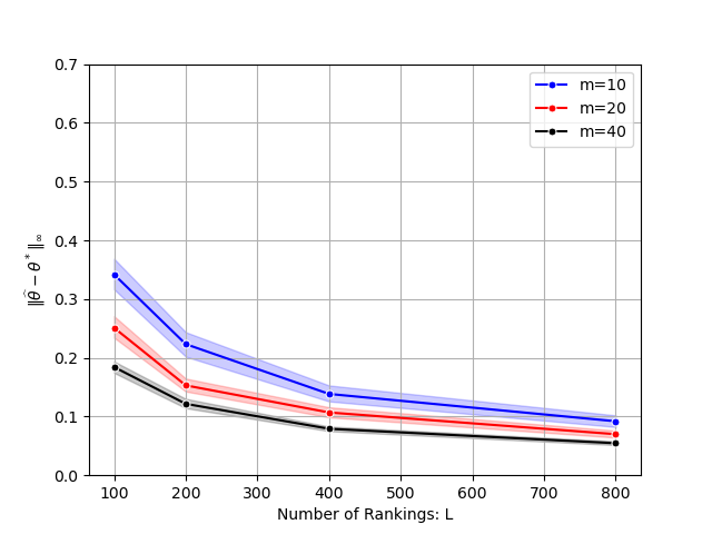
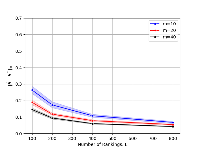
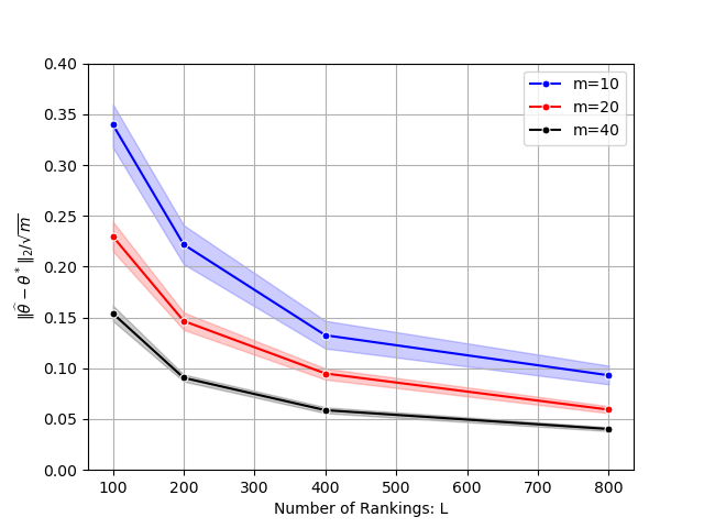
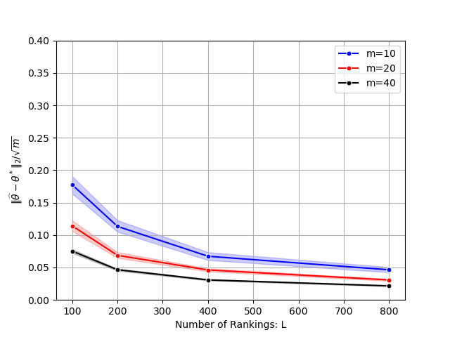
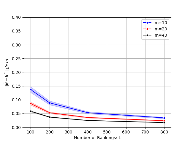
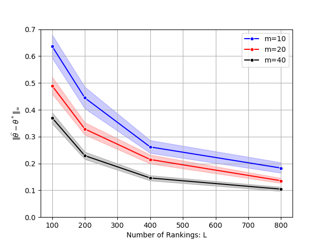
Scenario I. In the first scenario, we aim to provide empirical validations of the convergence of 𝜽^^𝜽\widehat{\bm{\theta}} to 𝜽superscript𝜽\bm{\theta}^{*} under constant privacy guarantee when m𝑚m or L𝐿L diverges. To this end, we consider cases (L,m){100,200,400,800}×{10,20,40}𝐿𝑚100200400800102040(L,m)\in\{100,200,400,800\}\times\{10,20,40\} with ϵ=1,2,3italic-ϵ123\epsilon=1,2,3. The regularization parameter is set as λL1(eϵ+1)2/(eϵ1)asymptotically-equals𝜆superscript𝐿1superscriptsuperscript𝑒italic-ϵ12superscript𝑒italic-ϵ1\lambda\asymp L^{-1}(e^{\epsilon}+1)^{2}/(e^{\epsilon}-1) as demonstrated in Theorem 1. In Figure 2, the averaged estimation errors, measured as 𝜽^𝜽subscriptnorm^𝜽superscript𝜽\|\widehat{\bm{\theta}}-\bm{\theta}^{*}\|_{\infty} and 𝜽^𝜽2/msubscriptnorm^𝜽superscript𝜽2𝑚\|\widehat{\bm{\theta}}-\bm{\theta}^{*}\|_{2}/\sqrt{m}, are reported, with each case being replicated 50 times. As depicted in Figure 2, when ϵitalic-ϵ\epsilon is set as a constant, the estimator 𝜽^^𝜽\widehat{\bm{\theta}} converges to 𝜽superscript𝜽\bm{\theta}^{*} as either L𝐿L or m𝑚m increases. This observation highlights that the estimator derived from the proposed debiased regularized M-estimator is a consistent estimator of 𝜽superscript𝜽\bm{\theta}^{*}, which aligns with our theoretical findings outlined in Theorem 1.
Refer to caption
(a) ϵitalic-ϵ\epsilon=1
Refer to caption
(b) ϵitalic-ϵ\epsilon=2
Refer to caption
(c) ϵitalic-ϵ\epsilon=3
Refer to caption
(d) ϵitalic-ϵ\epsilon=1
Refer to caption
(e) ϵitalic-ϵ\epsilon=2
Refer to caption
(f) ϵitalic-ϵ\epsilon=3
Figure 2: The averaged estimation errors of all cases in Scenario I, measured using 𝜽^𝜽subscriptnorm^𝜽superscript𝜽\|\widehat{\bm{\theta}}-\bm{\theta}^{*}\|_{\infty} and 𝜽^𝜽2/msubscriptnorm^𝜽superscript𝜽2𝑚\|\widehat{\bm{\theta}}-\bm{\theta}^{*}\|_{2}/\sqrt{m} and their corresponding 95% confidence intervals.

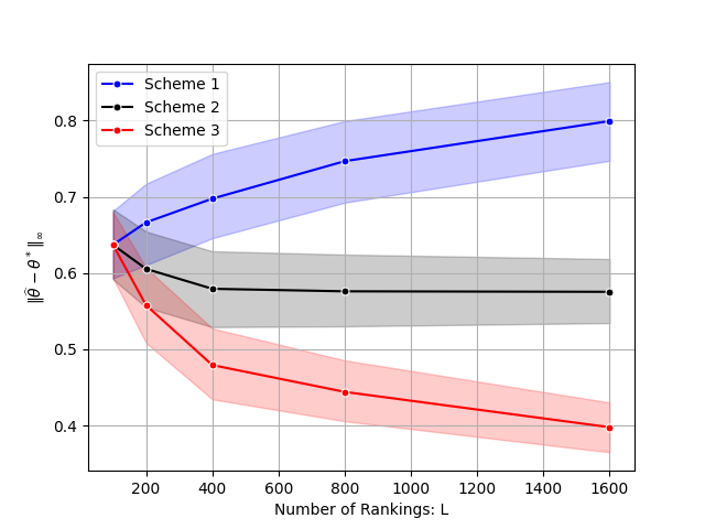
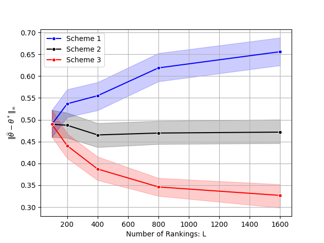
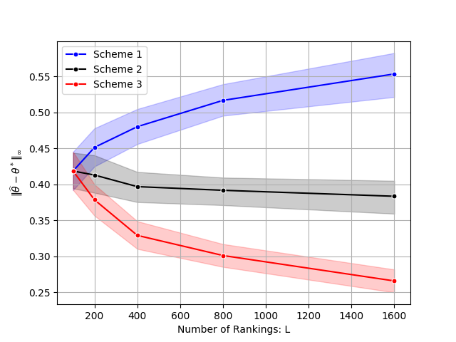
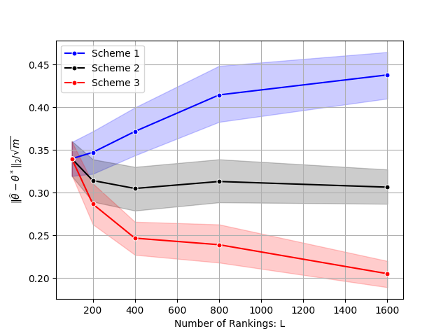
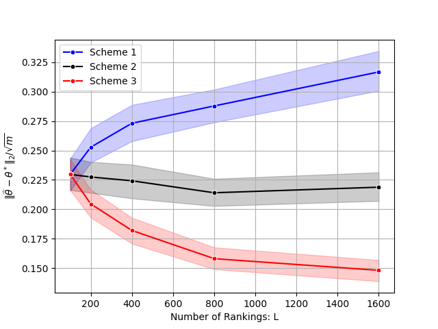
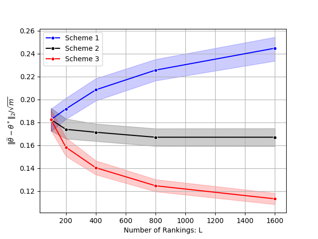
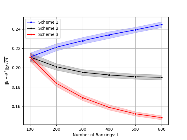
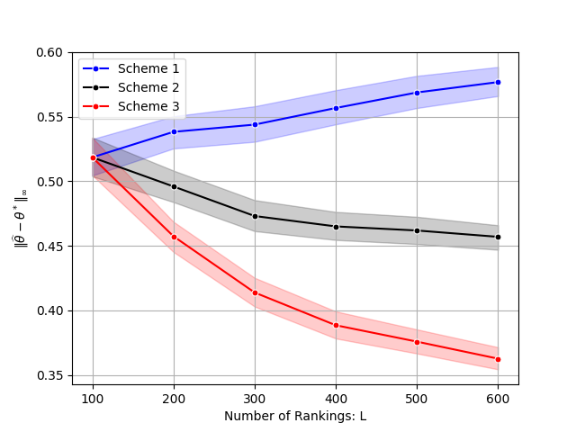
Scenario II. In the second scenario, we aim to verify our theoretical results that there exists an dividing line for the order of ϵitalic-ϵ\epsilon determining the convergence of 𝜽^^𝜽\widehat{\bm{\theta}} to 𝜽superscript𝜽\bm{\theta}^{*} when ϵitalic-ϵ\epsilon decreases with m𝑚m and L𝐿L. To this end, we consider cases (L,m){100,200,400,800,1600}×{10,20,30}𝐿𝑚1002004008001600102030(L,m)\in\{100,200,400,800,1600\}\times\{10,20,30\} under three data-dependent privacy schemes:

Scheme 1:ϵ1(m,L)log(mL)mL,:Scheme 1similar-tosubscriptitalic-ϵ1𝑚𝐿𝑚𝐿𝑚𝐿\displaystyle\mbox{Scheme 1}:\epsilon_{1}(m,L)\sim\frac{\log(mL)}{\sqrt{mL}},
Scheme 2:ϵ2(m,L)1mL,:Scheme 2similar-tosubscriptitalic-ϵ2𝑚𝐿1𝑚𝐿\displaystyle\mbox{Scheme 2}:\epsilon_{2}(m,L)\sim\frac{1}{\sqrt{mL}},
Scheme 3:ϵ3(m,L)1mLlog(mL),:Scheme 3similar-tosubscriptitalic-ϵ3𝑚𝐿1𝑚𝐿𝑚𝐿\displaystyle\mbox{Scheme 3}:\epsilon_{3}(m,L)\sim\frac{1}{\sqrt{mL}\log(mL)},

where the constants of three adaptive schemes are chosen such that ϵ1(m,100)=ϵ2(m,100)=ϵ3(m,100)=1subscriptitalic-ϵ1𝑚100subscriptitalic-ϵ2𝑚100subscriptitalic-ϵ3𝑚1001\epsilon_{1}(m,100)=\epsilon_{2}(m,100)=\epsilon_{3}(m,100)=1 for a given m𝑚m.

The estimation error of 𝜽^^𝜽\widehat{\bm{\theta}} is expected to display distinct patterns as L𝐿L or m𝑚m increases under three different schemes. Notably, the convergence of 𝜽^^𝜽\widehat{\bm{\theta}} towards the true parameter vector 𝜽superscript𝜽\bm{\theta}^{*} is not assured under Schemes 1 and 2, which becomes evident when we substitute ϵ1(m,L)subscriptitalic-ϵ1𝑚𝐿\epsilon_{1}(m,L) and ϵ2(m,L)subscriptitalic-ϵ2𝑚𝐿\epsilon_{2}(m,L) into the minimax lower bound as established in Theorem 3. Under Scheme 3, we can guarantee the convergence of 𝜽^^𝜽\widehat{\bm{\theta}}, which is supported by the upper bound presented in Theorem 1. Consequently, these schemes exhibit varying behaviors in terms of the estimation error of 𝜽^^𝜽\widehat{\bm{\theta}} as the values of L𝐿L or m𝑚m increase.

Refer to caption
(a) m=10𝑚10m=10
Refer to caption
(b) m=20𝑚20m=20
Refer to caption
(c) m=30𝑚30m=30
Refer to caption
(d) m=10𝑚10m=10
Refer to caption
(e) m=20𝑚20m=20
Refer to caption
(f) m=30𝑚30m=30
Figure 3: The averaged estimation errors of three privacy adaptive schemes in Scenario II, measured using 𝜽^𝜽subscriptnorm^𝜽superscript𝜽\|\widehat{\bm{\theta}}-\bm{\theta}^{*}\|_{\infty} in Figures (a) - (c) and 𝜽^𝜽2/msubscriptnorm^𝜽superscript𝜽2𝑚\|\widehat{\bm{\theta}}-\bm{\theta}^{*}\|_{2}/\sqrt{m} in Figures (d) - (f) and their corresponding 95% confidence intervals.

As depicted in Figure 3, the curve representing Scheme 2 remains unaltered as L𝐿L increases. This phenomenon arises from the delicate balance between the increase in information gain resulting from a higher number of rankings and the information loss due to enhanced privacy guarantee. Notably, the introduction of an additional logarithmic term exerts a substantial impact on the original curve pattern. More specifically, for Scheme 1, the estimation errors of 𝜽^^𝜽\widehat{\bm{\theta}} worsen considerably as L𝐿L increases, while in the case of Scheme 3, there is a significant improvement. Thus, it becomes evident that Scheme 2 appears as the threshold that determines whether the estimation error of 𝜽^^𝜽\widehat{\bm{\theta}} converges, aligning perfectly with our theoretical findings. This result matches with existing results regarding the parameter estimation under local differential privacy (Xu et al.,, 2023).

5.2 Ranking Recovery

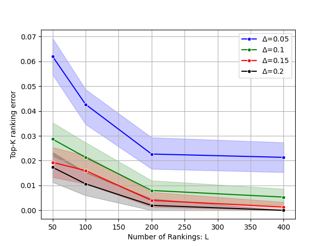
In this section, our primary objective is to assess the effectiveness of employing 𝜽^^𝜽\widehat{\bm{\theta}} for ranking recovery within the context of both fixed privacy guarantees and adaptive privacy schemes. Additionally, we aim to investigate how the disparity between the true preference parameters impacts the performance of ranking recovery. We assume that the true preference parameters are evenly spaced, denoted as 𝜽=(θ1,,θm)superscript𝜽superscriptsubscript𝜃1superscriptsubscript𝜃𝑚\bm{\theta}^{*}=(\theta_{1}^{*},\ldots,\theta_{m}^{*}), with a fixed interval, i.e., θ(i)θ(i1)=Δsuperscriptsubscript𝜃𝑖superscriptsubscript𝜃𝑖1Δ\theta_{(i)}^{*}-\theta_{(i-1)}^{*}=\Delta. The generation of pairwise rankings follows the same procedure as in the previous section.

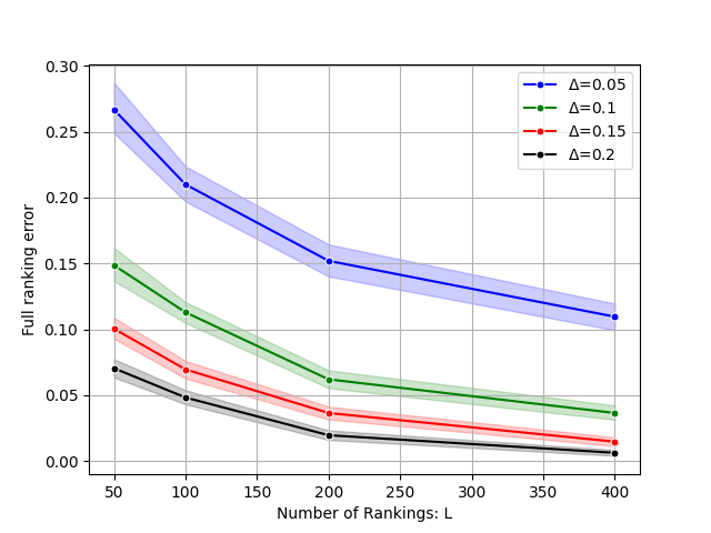
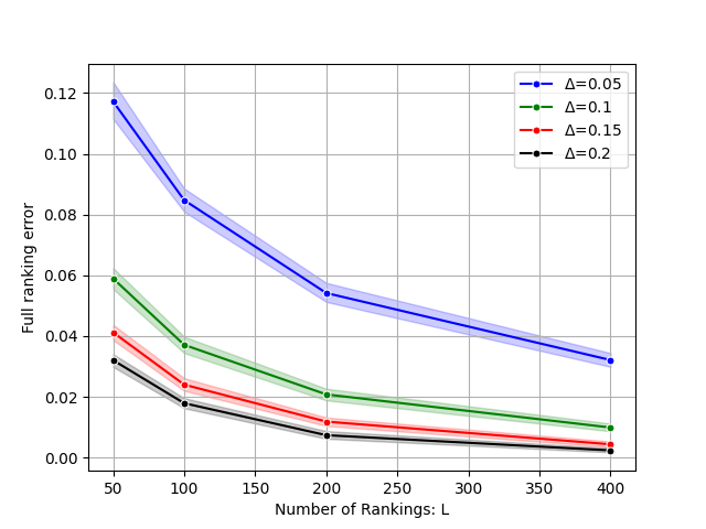
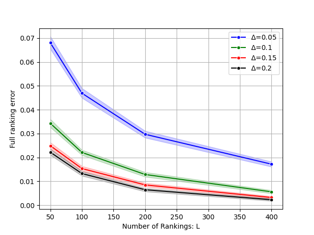
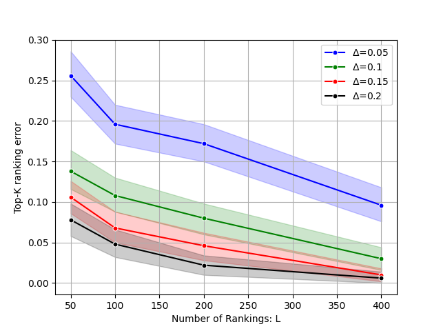
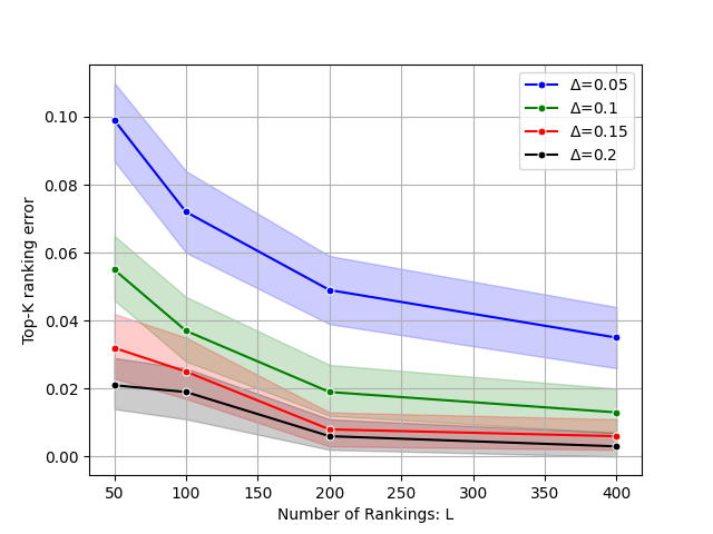
Scenario III. In this scenario, we aim to verify that ranking recovery is more attainable when either L𝐿L, m𝑚m, or ΔΔ\Delta goes to infinity. To this end, we consider cases (L,m,Δ){50,100,200,400}×{10,20,30}×{0.05,0.1,0.15,0.2}𝐿𝑚Δ501002004001020300.050.10.150.2(L,m,\Delta)\in\{50,100,200,400\}\times\{10,20,30\}\times\{0.05,0.1,0.15,0.2\} with ϵ=1italic-ϵ1\epsilon=1.

In Figure 4, we present the averaged top-K𝐾K ranking errors and full ranking errors across all cases. We set K𝐾K to be m/2𝑚2m/2 and replicate each case 100 times for constructing its 95% confidence interval. As depicted in Figure 4, we observe a clear trend of diminishing ranking errors as L𝐿L, m𝑚m, or ΔΔ\Delta increases. Comparing this trend to parameter estimation, it becomes evident that achieving a low ranking error is more attainable. Notably, when (n,m,Δ)=(400,30,0.2)𝑛𝑚Δ400300.2(n,m,\Delta)=(400,30,0.2), the full ranking error approaches almost zero, demonstrating a faster convergence rate compared with parameter estimation. This outcome is consistent with our theoretical findings outlined in Theorems 5 and 6.
Refer to caption
(a) m=10𝑚10m=10
Refer to caption
(b) m=20𝑚20m=20
Refer to caption
(c) m=30𝑚30m=30
Refer to caption
(d) m=10𝑚10m=10
Refer to caption
(e) m=20𝑚20m=20
Refer to caption
(f) m=30𝑚30m=30
Figure 4: The averaged top-K𝐾K ranking errors HK(𝜽^,𝜽)subscript𝐻𝐾^𝜽superscript𝜽H_{K}(\widehat{\bm{\theta}},\bm{\theta}^{*}) and full ranking errors K(𝜽^,𝜽)𝐾^𝜽superscript𝜽K(\widehat{\bm{\theta}},\bm{\theta}^{*}) of all cases in Scenario III and their corresponding 95% confidence intervals.

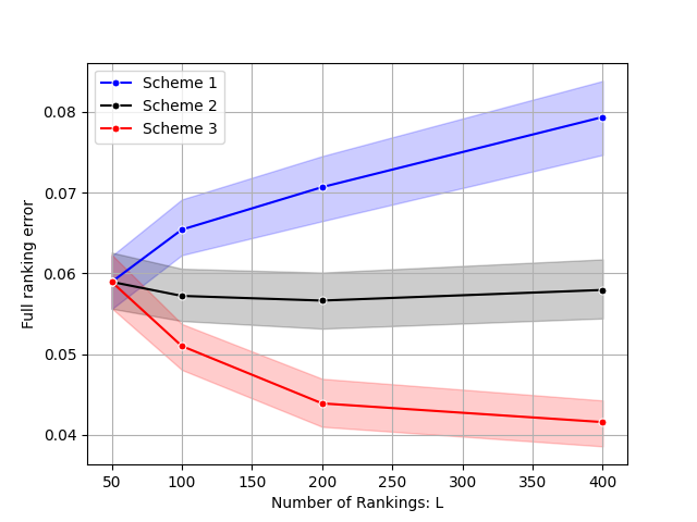
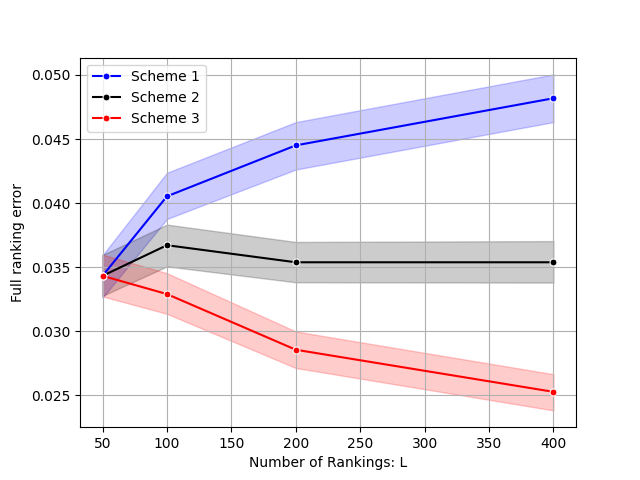
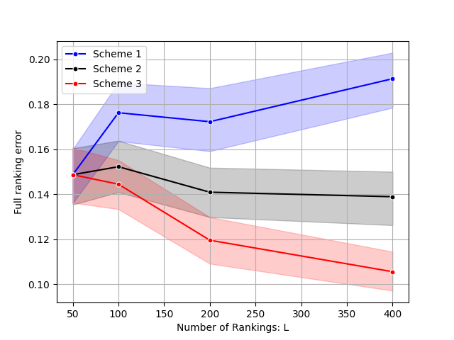
Scenario IV. In this scenario, we aim to verify that similar results as in Scenario II is observable for full ranking error that there exists a dividing line for the order of ϵitalic-ϵ\epsilon determining the convergence of the full ranking error when ϵitalic-ϵ\epsilon decreases with L𝐿L and m𝑚m. To this end, we consider cases (L,m){50,100,200,400}×{10,20,30}𝐿𝑚50100200400102030(L,m)\in\{50,100,200,400\}\times\{10,20,30\} under three data-dependent privacy schemes considered in Scenario II.
Refer to caption
(a) m=10𝑚10m=10
Refer to caption
(b) m=20𝑚20m=20
Refer to caption
(c) m=30𝑚30m=30
Figure 5: The averaged full ranking errors of three privacy adaptive schemes in Scenario IV and their corresponding 95% confidence intervals.

As illustrated in Figure 5, we observe a similar phenomenon for the full ranking error as in Figure 3. Again ϵ1mLasymptotically-equalsitalic-ϵ1𝑚𝐿\epsilon\asymp\frac{1}{\sqrt{mL}} appears as the dividing line that determines whether the full ranking error converges.

5.3 Efficiency of Debiased RR Mechanism

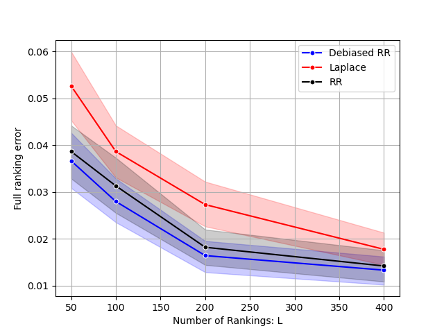
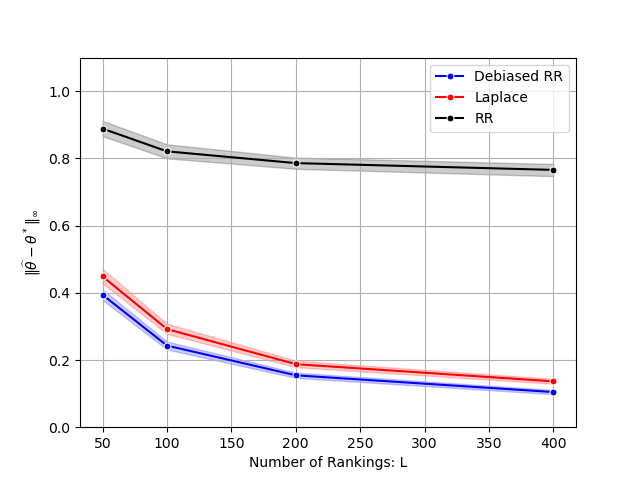
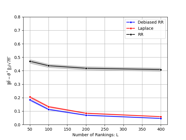
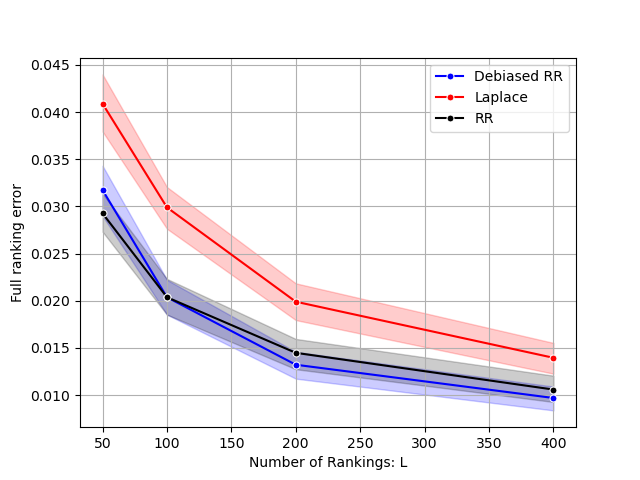
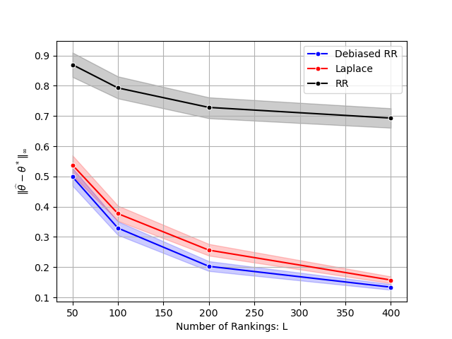
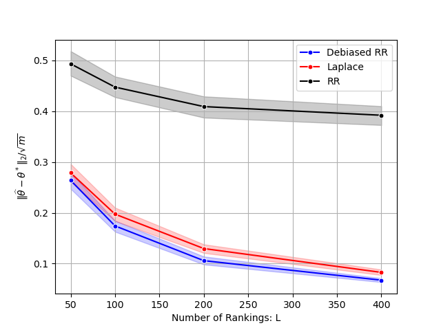
Scenario V. In this scenario, we undertake a comparison among the classic RR, debiased RR, and the Laplace mechanisms with the objective of demonstrating that privatized rankings achieved through the debiased RR mechanism maintain greater utility while ensuring the same level of privacy. This superiority stems from the precise alignment of the ϵitalic-ϵ\epsilon parameter in the RR mechanism with the disclosure risk, as highlighted in previous studies (Wasserman and Zhou,, 2010; Dong et al.,, 2022). Consequently, the debiased RR mechanism emerges as the optimal choice for protecting pairwise rankings. To this end, we consider cases (L,m){50,100,200,400}×{10,20}𝐿𝑚501002004001020(L,m)\in\{50,100,200,400\}\times\{10,20\} with ϵ=2italic-ϵ2\epsilon=2 and report the averaged full ranking error and estimation errors over 100 replications in Figure 6. The findings indicate that employing privatized rankings generated by the debiased RR mechanism enhances the performance of the rank aggregation task compared to those using the Laplace mechanism and the classic RR mechanism. Moreover, when implementing rank aggregation based on output rankings by the classic RR mechanism, achieving consistent estimation of 𝜽superscript𝜽\bm{\theta}^{*} becomes unattainable as anticipated. This stems from the fact that output rankings generated by the RR mechanism deviate from the underlying BTL model. Furthermore, the debiasing step not only rectifies this deviation but also enhances the utility in ranking items.
Refer to caption
(a) m=10,𝜽^𝜽𝑚10subscriptnorm^𝜽superscript𝜽m=10,\|\widehat{\bm{\theta}}-\bm{\theta}^{*}\|_{\infty}
Refer to caption
(b) m=10,m12𝜽^𝜽2𝑚10superscript𝑚12subscriptnorm^𝜽superscript𝜽2m=10,m^{-\frac{1}{2}}\|\widehat{\bm{\theta}}-\bm{\theta}^{*}\|_{2}
Refer to caption
(c) m=10,K(𝜽^,𝜽)𝑚10𝐾^𝜽superscript𝜽m=10,K(\widehat{\bm{\theta}},\bm{\theta}^{*})
Refer to caption
(d) m=20,𝜽^𝜽𝑚20subscriptnorm^𝜽superscript𝜽m=20,\|\widehat{\bm{\theta}}-\bm{\theta}^{*}\|_{\infty}
Refer to caption
(e) m=20,m12𝜽^𝜽2𝑚20superscript𝑚12subscriptnorm^𝜽superscript𝜽2m=20,m^{-\frac{1}{2}}\|\widehat{\bm{\theta}}-\bm{\theta}^{*}\|_{2}
Refer to caption
(f) m=20,K(𝜽^,𝜽)𝑚20𝐾^𝜽superscript𝜽m=20,K(\widehat{\bm{\theta}},\bm{\theta}^{*})
Figure 6: The comparison between the RR and Laplace mechanism using the full ranking error and estimation errors.

5.4 Real Experiment

In this section, we validate our theoretical results using the MovieLens 100K dataset. The MovieLens dataset we consider is collected by Harper and Konstan, (2015), containing 100,836 ratings from 610 users for 9,742 movies. The primary motivation behind this application is the concern that user interactions with items could potentially result in the exposure of personal information, including individual preferences and personal identity (McSherry and Mironov,, 2009; Gao et al.,, 2020). For illustration purposes, we only consider the 40 most-rated movies of this dataset, and our objective is to corroborate results similar to those obtained in Scenarios II and IV.

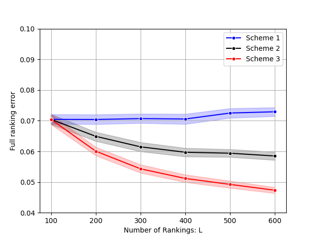
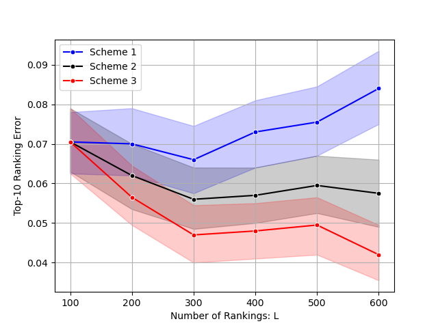
In the MovieLens dataset, item comparisons are generated by comparing ratings, and random comparisons are generated for two same ratings. Furthermore, items without ratings are considered less preferred. Since the true preference parameter vector for this dataset is unavailable, we fit the BTL model using the whole dataset and treat the resulting preference estimate as 𝜽superscript𝜽\bm{\theta}^{*}. We explore various sample sizes and consider three adaptive privacy schemes, as defined in Scenario II. The full ranking error, top-10 ranking error, and estimation errors over 200 replications are reported in (a)-(d) of Figure 7, respectively.
Refer to caption
(a) K(𝜽^,𝜽)𝐾bold-^𝜽superscript𝜽K(\bm{\widehat{\theta}},\bm{\theta}^{*})
Refer to caption
(b) H10(𝜽^,𝜽)subscript𝐻10bold-^𝜽superscript𝜽H_{10}(\bm{\widehat{\theta}},\bm{\theta}^{*})
Refer to caption
(c) m12𝜽^𝜽2superscript𝑚12subscriptnormbold-^𝜽superscript𝜽2m^{-\frac{1}{2}}\|\bm{\widehat{\theta}}-\bm{\theta}^{*}\|_{2}
Refer to caption
(d) 𝜽^𝜽subscriptnormbold-^𝜽superscript𝜽\|\bm{\widehat{\theta}}-\bm{\theta}^{*}\|_{\infty}
Figure 7: The averaged errors under three adaptive privacy schemes and various sizes of data and the starting point denotes the case ϵ=1italic-ϵ1\epsilon=1 for three schemes.

As illustrated in Figure 7, we note a similar phenomenon to that observed in the simulations. Specifically, there is a significant rise in ranking errors and estimation errors in Scheme 1, while conversely, a decreasing trend is evident under Scheme 3. This bolsters our conclusion regarding the presence of a clear boundary that dictates the convergence of utility within the rank aggregation task context. This distinct boundary implies the optimal tradeoff between privacy and utility in our rank aggregation framework.

References

  • Ackerman et al., (2013) Ackerman, M., Choi, S.-Y., Coughlin, P., Gottlieb, E., and Wood, J. (2013). Elections with partially ordered preferences. Public Choice, 157:145–168.
  • Alabi et al., (2022) Alabi, D., Ghazi, B., Kumar, R., and Manurangsi, P. (2022). Private rank aggregation in central and local models. In Proceedings of the AAAI Conference on Artificial Intelligence, volume 36, pages 5984–5991.
  • Arachchige et al., (2019) Arachchige, P. C. M., Bertok, P., Khalil, I., Liu, D., Camtepe, S., and Atiquzzaman, M. (2019). Local differential privacy for deep learning. IEEE Internet of Things Journal, 7(7):5827–5842.
  • Bi and Shen, (2023) Bi, X. and Shen, X. (2023). Distribution-invariant differential privacy. Journal of econometrics, 235(2):444–453.
  • Bradley and Terry, (1952) Bradley, R. A. and Terry, M. E. (1952). Rank analysis of incomplete block designs: I. the method of paired comparisons. Biometrika, 39(3/4):324–345.
  • Cai et al., (2021) Cai, T. T., Wang, Y., and Zhang, L. (2021). The cost of privacy: Optimal rates of convergence for parameter estimation with differential privacy. The Annals of Statistics, 49(5):2825–2850.
  • Carlson and Montgomery, (2017) Carlson, D. and Montgomery, J. M. (2017). A pairwise comparison framework for fast, flexible, and reliable human coding of political texts. American Political Science Review, 111(4):835–843.
  • Chen et al., (2022) Chen, P., Gao, C., and Zhang, A. Y. (2022). Partial recovery for top-k𝑘k ranking: optimality of MLE, and suboptimality of the spectral method. The Annals of Statistics, 50(3):1618–1652.
  • Chen et al., (2019) Chen, Y., Fan, J., Ma, C., and Wang, K. (2019). Spectral method and regularized mle are both optimal for top-k ranking. Annals of statistics, 47(4):2204.
  • Chen and Suh, (2015) Chen, Y. and Suh, C. (2015). Spectral mle: Top-k rank aggregation from pairwise comparisons. In International Conference on Machine Learning, pages 371–380. PMLR.
  • Chhor and Sentenac, (2023) Chhor, J. and Sentenac, F. (2023). Robust estimation of discrete distributions under local differential privacy. In International Conference on Algorithmic Learning Theory, pages 411–446. PMLR.
  • Costante et al., (2013) Costante, E., Paci, F., and Zannone, N. (2013). Privacy-aware web service composition and ranking. In 2013 IEEE 20th International Conference on Web Services, pages 131–138. IEEE.
  • Dong et al., (2022) Dong, J., Roth, A., and Su, W. J. (2022). Gaussian differential privacy. Journal of the Royal Statistical Society Series B, 84(1):3–37.
  • Duchi et al., (2018) Duchi, J. C., Jordan, M. I., and Wainwright, M. J. (2018). Minimax optimal procedures for locally private estimation. Journal of the American Statistical Association, 113(521):182–201.
  • Dwork, (2006) Dwork, C. (2006). Differential privacy. In International Colloquium on Automata, Languages, and Programming, pages 1–12. Springer.
  • Dwork et al., (2001) Dwork, C., Kumar, R., Naor, M., and Sivakumar, D. (2001). Rank aggregation methods for the web. In Proceedings of the 10th International Conference on World Wide Web, pages 613–622.
  • Dwork and Roth, (2014) Dwork, C. and Roth, A. (2014). The algorithmic foundations of differential privacy. Foundations and Trends® in Theoretical Computer Science, 9(3–4):211–407.
  • Erlingsson et al., (2014) Erlingsson, Ú., Pihur, V., and Korolova, A. (2014). Rappor: Randomized aggregatable privacy-preserving ordinal response. In Proceedings of the 2014 ACM SIGSAC Conference on Computer and Communications Security, pages 1054–1067.
  • Gao et al., (2020) Gao, C., Huang, C., Lin, D., Jin, D., and Li, Y. (2020). Dplcf: differentially private local collaborative filtering. In Proceedings of the 43rd International ACM SIGIR Conference on Research and Development in Information Retrieval, pages 961–970.
  • Gao et al., (2023) Gao, C., Shen, Y., and Zhang, A. Y. (2023). Uncertainty quantification in the bradley–terry–luce model. Information and Inference: A Journal of the IMA, 12(2):1073–1140.
  • Hajek et al., (2014) Hajek, B., Oh, S., and Xu, J. (2014). Minimax-optimal inference from partial rankings. Advances in Neural Information Processing Systems, 27.
  • Harper and Konstan, (2015) Harper, F. M. and Konstan, J. A. (2015). The movielens datasets: History and context. Acm transactions on interactive intelligent systems (tiis), 5(4):1–19.
  • Hay et al., (2017) Hay, M., Elagina, L., and Miklau, G. (2017). Differentially private rank aggregation. In Proceedings of the 2017 SIAM International Conference on Data Mining, pages 669–677. SIAM.
  • Ichihashi, (2020) Ichihashi, S. (2020). Online privacy and information disclosure by consumers. American Economic Review, 110(2):569–595.
  • Jeong et al., (2022) Jeong, M., Dytso, A., and Cardone, M. (2022). Ranking recovery under privacy considerations. Transactions on Machine Learning Research.
  • Kalloori et al., (2018) Kalloori, S., Ricci, F., and Gennari, R. (2018). Eliciting pairwise preferences in recommender systems. In Proceedings of the 12th ACM Conference on Recommender Systems, pages 329–337.
  • Karatzoglou et al., (2013) Karatzoglou, A., Baltrunas, L., and Shi, Y. (2013). Learning to rank for recommender systems. In Proceedings of the 7th ACM Conference on Recommender Systems, pages 493–494.
  • Karlé and Tyagi, (2023) Karlé, E. and Tyagi, H. (2023). Dynamic ranking with the btl model: a nearest neighbor based rank centrality method. Journal of Machine Learning Research, 24(269):1–57.
  • Klein and Rio, (2005) Klein, T. and Rio, E. (2005). Concentration around the mean for maxima of empirical processes. The Annals of Probability, 33(3):1060–1077.
  • Koltchinskii, (2011) Koltchinskii, V. (2011). Oracle inequalities in empirical risk minimization and sparse recovery problems: École D’Été de Probabilités de Saint-Flour XXXVIII-2008, volume 2033. Springer Science & Business Media.
  • Lee, (2015) Lee, D. T. (2015). Efficient, private, and eps-strategyproof elicitation of tournament voting rules. In Twenty-Fourth International Joint Conference on Artificial Intelligence.
  • Li et al., (2023) Li, Z., Liu, A., Xia, L., Cao, Y., and Wang, H. (2023). Differentially private condorcet voting. In Proceedings of the AAAI Conference on Artificial Intelligence, volume 37, pages 5755–5763.
  • Liu et al., (2023) Liu, Y., Fang, E. X., and Lu, J. (2023). Lagrangian inference for ranking problems. Operations Research, 71(1):202–223.
  • Liu et al., (2007) Liu, Y.-T., Liu, T.-Y., Qin, T., Ma, Z.-M., and Li, H. (2007). Supervised rank aggregation. In Proceedings of the 16th International Conference on World Wide Web, pages 481–490.
  • Luce, (2012) Luce, R. D. (2012). Individual choice behavior: A theoretical analysis. Courier Corporation.
  • McCarthy and Santucci, (2021) McCarthy, D. and Santucci, J. (2021). Ranked choice voting as a generational issue in modern american politics. Politics & Policy, 49(1):33–60.
  • McSherry and Mironov, (2009) McSherry, F. and Mironov, I. (2009). Differentially private recommender systems: Building privacy into the netflix prize contenders. In Proceedings of the 15th ACM SIGKDD international conference on Knowledge discovery and data mining, pages 627–636.
  • Negahban et al., (2016) Negahban, S., Oh, S., and Shah, D. (2016). Rank centrality: Ranking from pairwise com-parisons. Operations Research, 65(1):266–287.
  • Nielson, (2017) Nielson, L. (2017). Ranked choice voting and attitudes toward democracy in the united states: Results from a survey experiment. Politics & Policy, 45(4):535–570.
  • Okazaki et al., (2009) Okazaki, S., Li, H., and Hirose, M. (2009). Consumer privacy concerns and preference for degree of regulatory control. Journal of Advertising, 38(4):63–77.
  • Oliveira et al., (2020) Oliveira, S. E., Diniz, V., Lacerda, A., Merschmanm, L., and Pappa, G. L. (2020). Is rank aggregation effective in recommender systems? an experimental analysis. ACM Transactions on Intelligent Systems and Technology (TIST), 11(2):1–26.
  • Shah and Wainwright, (2018) Shah, N. B. and Wainwright, M. J. (2018). Simple, robust and optimal ranking from pairwise comparisons. Journal of Machine Learning Research, 18(199):1–38.
  • Shang et al., (2014) Shang, S., Wang, T., Cuff, P., and Kulkarni, S. (2014). The application of differential privacy for rank aggregation: Privacy and accuracy. In 17th International Conference on Information Fusion (FUSION), pages 1–7. IEEE.
  • Shen et al., (2023) Shen, X., Liu, Y., and Shen, R. (2023). Boosting data analytics with synthetic volume expansion. arXiv preprint arXiv:2310.17848.
  • Suh et al., (2017) Suh, C., Tan, V. Y., and Zhao, R. (2017). Adversarial top-k𝑘k ranking. IEEE Transactions on Information Theory, 63(4):2201–2225.
  • Szörényi et al., (2015) Szörényi, B., Busa-Fekete, R., Paul, A., and Hüllermeier, E. (2015). Online rank elicitation for plackett-luce: A dueling bandits approach. Advances in Neural Information Processing Systems, 28.
  • Tang et al., (2017) Tang, J., Korolova, A., Bai, X., Wang, X., and Wang, X. (2017). Privacy loss in apple’s implementation of differential privacy on macos 10.12. arXiv preprint arXiv:1709.02753.
  • Van Erven and Harremos, (2014) Van Erven, T. and Harremos, P. (2014). Rényi divergence and kullback-leibler divergence. IEEE Transactions on Information Theory, 60(7):3797–3820.
  • Wang and Xu, (2019) Wang, D. and Xu, J. (2019). On sparse linear regression in the local differential privacy model. In International Conference on Machine Learning, pages 6628–6637. PMLR.
  • Wang et al., (2017) Wang, T., Blocki, J., Li, N., and Jha, S. (2017). Locally differentially private protocols for frequency estimation. In 26th USENIX Security Symposium (USENIX Security 17), pages 729–745.
  • Warner, (1965) Warner, S. L. (1965). Randomized response: A survey technique for eliminating evasive answer bias. Journal of the American Statistical Association, 60(309):63–69.
  • Wasserman and Zhou, (2010) Wasserman, L. and Zhou, S. (2010). A statistical framework for differential privacy. Journal of the American Statistical Association, 105(489):375–389.
  • Xia et al., (2020) Xia, R., Tan, V. Y., Filstroff, L., and Févotte, C. (2020). A ranking model motivated by nonnegative matrix factorization with applications to tennis tournaments. In Machine Learning and Knowledge Discovery in Databases: European Conference, ECML PKDD 2019, Würzburg, Germany, September 16–20, 2019, Proceedings, Part III, pages 187–203. Springer.
  • Xu et al., (2023) Xu, S., Wang, C., Sun, W. W., and Cheng, G. (2023). Binary classification under local label differential privacy using randomized response mechanisms. Transactions on Machine Learning Research.
  • Yan et al., (2020) Yan, Z., Li, G., and Liu, J. (2020). Private rank aggregation under local differential privacy. International Journal of Intelligent Systems, 35(10):1492–1519.
  • Yang et al., (2020) Yang, M., Lyu, L., Zhao, J., Zhu, T., and Lam, K.-Y. (2020). Local differential privacy and its applications: A comprehensive survey. arXiv preprint arXiv:2008.03686.
  • Zhu et al., (2023) Zhu, B., Jiao, J., and Jordan, M. I. (2023). Principled reinforcement learning with human feedback from pairwise or k𝑘k-wise comparisons. arXiv preprint arXiv:2301.11270.

Supplementary Materials

“Rate-Optimal Rank Aggregation with Private Pairwise Rankings ”


In this supplementary file, we provide detailed proofs for all lemmas in Section S.1, all theorems in Section S.2, all corollaries in Section S.3.

S.1 Proof of Lemmas

Proof of Lemma 1: By the definition of Yijsubscript𝑌𝑖𝑗Y_{ij}, we have

(Y~ij=1)=subscript~𝑌𝑖𝑗1absent\displaystyle\mathbb{P}\big{(}\widetilde{Y}_{ij}=1\big{)}= (Yij=1)(1pϵ)+(Yij=0)pϵsubscript𝑌𝑖𝑗11subscript𝑝italic-ϵsubscript𝑌𝑖𝑗0subscript𝑝italic-ϵ\displaystyle\mathbb{P}\left(Y_{ij}=1\right)(1-p_{\epsilon})+\mathbb{P}\left(Y_{ij}=0\right)p_{\epsilon}
=\displaystyle= eθieθi+eθj(1pϵ)+eθjeθi+eθjpϵsuperscript𝑒superscriptsubscript𝜃𝑖superscript𝑒superscriptsubscript𝜃𝑖superscript𝑒superscriptsubscript𝜃𝑗1subscript𝑝italic-ϵsuperscript𝑒superscriptsubscript𝜃𝑗superscript𝑒superscriptsubscript𝜃𝑖superscript𝑒superscriptsubscript𝜃𝑗subscript𝑝italic-ϵ\displaystyle\frac{e^{\theta_{i}^{*}}}{e^{\theta_{i}^{*}}+e^{\theta_{j}^{*}}}(1-p_{\epsilon})+\frac{e^{\theta_{j}^{*}}}{e^{\theta_{i}^{*}}+e^{\theta_{j}^{*}}}p_{\epsilon}
=\displaystyle= 12+eθieθjeθi+eθj(1/2pϵ).12superscript𝑒superscriptsubscript𝜃𝑖superscript𝑒superscriptsubscript𝜃𝑗superscript𝑒superscriptsubscript𝜃𝑖superscript𝑒superscriptsubscript𝜃𝑗12subscript𝑝italic-ϵ\displaystyle\frac{1}{2}+\frac{e^{\theta_{i}^{*}}-e^{\theta_{j}^{*}}}{e^{\theta_{i}^{*}}+e^{\theta_{j}^{*}}}(1/2-p_{\epsilon}).

This completes the proof. ∎

Proof of Lemma 2: For each l[L]𝑙delimited-[]𝐿l\in[L] and ij𝑖𝑗i\neq j, we have

𝔼((eϵl+1)y~ij(l)1eϵl1)=𝔼superscript𝑒subscriptitalic-ϵ𝑙1superscriptsubscript~𝑦𝑖𝑗𝑙1superscript𝑒subscriptitalic-ϵ𝑙1absent\displaystyle\mathbb{E}\left(\frac{(e^{\epsilon_{l}}+1)\widetilde{y}_{ij}^{(l)}-1}{e^{\epsilon_{l}}-1}\right)= eϵl+1eϵl1(12+12eθieθjeθi+eθj(eϵl1eϵl+1))1eϵl1superscript𝑒subscriptitalic-ϵ𝑙1superscript𝑒subscriptitalic-ϵ𝑙11212superscript𝑒superscriptsubscript𝜃𝑖superscript𝑒superscriptsubscript𝜃𝑗superscript𝑒superscriptsubscript𝜃𝑖superscript𝑒superscriptsubscript𝜃𝑗superscript𝑒subscriptitalic-ϵ𝑙1superscript𝑒subscriptitalic-ϵ𝑙11superscript𝑒subscriptitalic-ϵ𝑙1\displaystyle\frac{e^{\epsilon_{l}}+1}{e^{\epsilon_{l}}-1}\left(\frac{1}{2}+\frac{1}{2}\frac{e^{\theta_{i}^{*}}-e^{\theta_{j}^{*}}}{e^{\theta_{i}^{*}}+e^{\theta_{j}^{*}}}\left(\frac{e^{\epsilon_{l}}-1}{e^{\epsilon_{l}}+1}\right)\right)-\frac{1}{e^{\epsilon_{l}}-1}
=\displaystyle= 12+12eθieθjeθi+eθj=eθieθi+eθj.1212superscript𝑒superscriptsubscript𝜃𝑖superscript𝑒superscriptsubscript𝜃𝑗superscript𝑒superscriptsubscript𝜃𝑖superscript𝑒superscriptsubscript𝜃𝑗superscript𝑒superscriptsubscript𝜃𝑖superscript𝑒superscriptsubscript𝜃𝑖superscript𝑒superscriptsubscript𝜃𝑗\displaystyle\frac{1}{2}+\frac{1}{2}\frac{e^{\theta_{i}^{*}}-e^{\theta_{j}^{*}}}{e^{\theta_{i}^{*}}+e^{\theta_{j}^{*}}}=\frac{e^{\theta_{i}^{*}}}{e^{\theta_{i}^{*}}+e^{\theta_{j}^{*}}}.

As for the variance,

Var(zij(l))=(eϵl+1eϵl1)2Var(y~ij(l))=(eϵl+1eϵl1)2(1414(eϵ1eϵ+1eθieθjeθi+eθj)2).Varsuperscriptsubscript𝑧𝑖𝑗𝑙superscriptsuperscript𝑒subscriptitalic-ϵ𝑙1superscript𝑒subscriptitalic-ϵ𝑙12Varsuperscriptsubscript~𝑦𝑖𝑗𝑙superscriptsuperscript𝑒subscriptitalic-ϵ𝑙1superscript𝑒subscriptitalic-ϵ𝑙121414superscriptsuperscript𝑒italic-ϵ1superscript𝑒italic-ϵ1superscript𝑒superscriptsubscript𝜃𝑖superscript𝑒superscriptsubscript𝜃𝑗superscript𝑒superscriptsubscript𝜃𝑖superscript𝑒superscriptsubscript𝜃𝑗2\displaystyle\text{Var}\left(z_{ij}^{(l)}\right)=\left(\frac{e^{\epsilon_{l}}+1}{e^{\epsilon_{l}}-1}\right)^{2}\text{Var}\left(\widetilde{y}_{ij}^{(l)}\right)=\left(\frac{e^{\epsilon_{l}}+1}{e^{\epsilon_{l}}-1}\right)^{2}\left(\frac{1}{4}-\frac{1}{4}\left(\frac{e^{\epsilon}-1}{e^{\epsilon}+1}\frac{e^{\theta_{i}^{*}}-e^{\theta_{j}^{*}}}{e^{\theta_{i}^{*}}+e^{\theta_{j}^{*}}}\right)^{2}\right).

This completes the proof. ∎

Proof of Lemma 3: We first note that λ(𝜽)=0(𝜽)+λ𝜽22subscript𝜆𝜽subscript0𝜽𝜆superscriptsubscriptnorm𝜽22\mathcal{L}_{\lambda}(\bm{\theta})=\mathcal{L}_{0}(\bm{\theta})+\lambda\|\bm{\theta}\|_{2}^{2}. Let 𝒈=(g1,,gm1)m1𝒈subscript𝑔1subscript𝑔𝑚1superscript𝑚1\bm{g}=(g_{1},\ldots,g_{m-1})\in\mathbb{R}^{m-1}, then we define

𝚯(𝒈)={𝜽m:θiθi+1=gi, for i[m1]}.𝚯𝒈conditional-set𝜽superscript𝑚formulae-sequencesubscript𝜃𝑖subscript𝜃𝑖1subscript𝑔𝑖 for 𝑖delimited-[]𝑚1\displaystyle\bm{\Theta}(\bm{g})=\big{\{}\bm{\theta}\in\mathbb{R}^{m}:\theta_{i}-\theta_{i+1}=g_{i},\text{ for }i\in[m-1]\big{\}}.

Notice that 0(𝜽)subscript0𝜽\mathcal{L}_{0}(\bm{\theta}) stays invariant to translation for any fixed 𝜽𝜽\bm{\theta}. In other words, 0(𝜽)=0(𝜽+C𝟏)subscript0𝜽subscript0𝜽𝐶1\mathcal{L}_{0}(\bm{\theta})=\mathcal{L}_{0}(\bm{\theta}+C\bm{1}) for any constant C𝐶C. Therefore, for any 𝜽1,𝜽2𝚯(𝒈)subscript𝜽1subscript𝜽2𝚯𝒈\bm{\theta}_{1},\bm{\theta}_{2}\in\bm{\Theta}(\bm{g}), we have 0(𝜽1)=0(𝜽2)subscript0subscript𝜽1subscript0subscript𝜽2\mathcal{L}_{0}(\bm{\theta}_{1})=\mathcal{L}_{0}(\bm{\theta}_{2}). With this, for any 𝜽+C𝟏𝚯(𝒈)𝜽𝐶1𝚯𝒈\bm{\theta}+C\bm{1}\in\bm{\Theta}(\bm{g}),

𝜽+C𝟏22=𝜽22+2Ci=1mθi+mC2.superscriptsubscriptnorm𝜽𝐶122superscriptsubscriptnorm𝜽222𝐶superscriptsubscript𝑖1𝑚subscript𝜃𝑖𝑚superscript𝐶2\displaystyle\|\bm{\theta}+C\bm{1}\|_{2}^{2}=\|\bm{\theta}\|_{2}^{2}+2C\sum_{i=1}^{m}\theta_{i}+mC^{2}. (S1)

Clearly, (S1) is minimized when C=1mi=1mθi𝐶1𝑚superscriptsubscript𝑖1𝑚subscript𝜃𝑖C=-\frac{1}{m}\sum_{i=1}^{m}\theta_{i}. Therefore, for any 𝒈m1𝒈superscript𝑚1\bm{g}\in\mathbb{R}^{m-1}, we have

𝜽0θ0¯𝟏=argmin𝜽𝚯(𝒈){0(𝜽)+λ𝜽22},subscript𝜽0¯subscript𝜃01subscriptargmin𝜽𝚯𝒈conditional-setsubscript0𝜽𝜆evaluated-at𝜽22\displaystyle\bm{\theta}_{0}-\overline{\theta_{0}}\bm{1}=\mathop{\mathrm{argmin}}_{\bm{\theta}\in\bm{\Theta}(\bm{g})}\left\{\mathcal{L}_{0}(\bm{\theta})+\lambda\|\bm{\theta}\|_{2}^{2}\right\},

where 𝜽0subscript𝜽0\bm{\theta}_{0} is any vector in 𝚯(𝒈)𝚯𝒈\bm{\Theta}(\bm{g}) and θ¯0=1mi=1mθ0isubscript¯𝜃01𝑚superscriptsubscript𝑖1𝑚subscript𝜃0𝑖\overline{\theta}_{0}=\frac{1}{m}\sum_{i=1}^{m}\theta_{0i}. It then follows that 𝟏T𝜽^=0superscript1𝑇^𝜽0\bm{1}^{T}\widehat{\bm{\theta}}=0, which completes the proof. ∎

Proof of Lemma 4: The proof of Lemma 4 is a direct application of Lemma 3.1 of Chen et al., (2022). Using Lemma 3.1 of Chen et al., (2022), we have

HK(𝜽^,𝜽)1Kmint[i:σ(θi)KI(θ^it)+i:σ(θi)>KI(θ^it)].subscript𝐻𝐾^𝜽superscript𝜽1𝐾subscript𝑡subscript:𝑖𝜎superscriptsubscript𝜃𝑖𝐾𝐼subscript^𝜃𝑖𝑡subscript:𝑖𝜎superscriptsubscript𝜃𝑖𝐾𝐼subscript^𝜃𝑖𝑡\displaystyle H_{K}(\widehat{\bm{\theta}},\bm{\theta}^{*})\leq\frac{1}{K}\min_{t\in\mathbb{R}}\left[\sum_{i:\sigma(\theta_{i}^{*})\leq K}I\left(\widehat{\theta}_{i}\leq t\right)+\sum_{i:\sigma(\theta_{i}^{*})>K}I\left(\widehat{\theta}_{i}\geq t\right)\right].

Taking the expectation of both sides, we get

𝔼(HK(𝜽^,𝜽))1Kmint[i:σ(θi)KI(θ^it)+i:σ(θi)>KI(θ^it)].𝔼subscript𝐻𝐾^𝜽superscript𝜽1𝐾subscript𝑡subscript:𝑖𝜎superscriptsubscript𝜃𝑖𝐾𝐼subscript^𝜃𝑖𝑡subscript:𝑖𝜎superscriptsubscript𝜃𝑖𝐾𝐼subscript^𝜃𝑖𝑡\displaystyle\mathbb{E}\left(H_{K}(\widehat{\bm{\theta}},\bm{\theta}^{*})\right)\leq\frac{1}{K}\min_{t\in\mathbb{R}}\left[\sum_{i:\sigma(\theta_{i}^{*})\leq K}I\left(\widehat{\theta}_{i}\leq t\right)+\sum_{i:\sigma(\theta_{i}^{*})>K}I\left(\widehat{\theta}_{i}\geq t\right)\right].

The desired result immediately follows by taking t=θ(K)+θ(K+1)2𝑡superscriptsubscript𝜃𝐾superscriptsubscript𝜃𝐾12t=\frac{\theta_{(K)}^{*}+\theta_{(K+1)}^{*}}{2}. ∎

Lemma S5 (Strong convexity of λ(𝜽)subscript𝜆𝜽\mathcal{L}_{\lambda}(\bm{\theta})).

The Hessian matrix of 𝓛𝛌(𝛉)subscript𝓛𝛌𝛉\bm{\mathcal{L}_{\lambda}(\bm{\theta})} is given as

2λ(𝜽)=i<jeθieθj(eθi+eθj)2(𝒆i𝒆j)(𝒆i𝒆j)T+2λ𝑰m.superscript2subscript𝜆𝜽subscript𝑖𝑗superscript𝑒subscript𝜃𝑖superscript𝑒subscript𝜃𝑗superscriptsuperscript𝑒subscript𝜃𝑖superscript𝑒subscript𝜃𝑗2subscript𝒆𝑖subscript𝒆𝑗superscriptsubscript𝒆𝑖subscript𝒆𝑗𝑇2𝜆subscript𝑰𝑚\displaystyle\nabla^{2}\mathcal{L}_{\lambda}(\bm{\theta})=\sum_{i<j}\frac{e^{\theta_{i}}e^{\theta_{j}}}{(e^{\theta_{i}}+e^{\theta_{j}})^{2}}(\bm{e}_{i}-\bm{e}_{j})(\bm{e}_{i}-\bm{e}_{j})^{T}+2\lambda\bm{I}_{m}.

Let Λl(2(𝛉))subscriptΛ𝑙superscript2𝛉\Lambda_{l}(\nabla^{2}\mathcal{L}(\bm{\theta})) denote the l𝑙l-th largest eigenvalue of 2(𝛉)superscript2𝛉\nabla^{2}\mathcal{L}(\bm{\theta}). For any 𝛉p𝛉superscript𝑝\bm{\theta}\in\mathbb{R}^{p}, it holds that

2λΛl(2λ(𝜽))2(λ+maxi[m]jieθieθj(eθi+eθj)2),2𝜆subscriptΛ𝑙superscript2subscript𝜆𝜽2𝜆subscript𝑖delimited-[]𝑚subscript𝑗𝑖superscript𝑒subscript𝜃𝑖superscript𝑒subscript𝜃𝑗superscriptsuperscript𝑒subscript𝜃𝑖superscript𝑒subscript𝜃𝑗2\displaystyle 2\lambda\leq\Lambda_{l}(\nabla^{2}\mathcal{L}_{\lambda}(\bm{\theta}))\leq 2\Big{(}\lambda+\max_{i\in[m]}\sum_{j\neq i}\frac{e^{\theta_{i}}e^{\theta_{j}}}{(e^{\theta_{i}}+e^{\theta_{j}})^{2}}\Big{)},

for any l=1,,m𝑙1𝑚l=1,\ldots,m.

Proof of Lemma S5: The proof presented here is similar to that of Lemma 6.3 in (Chen et al.,, 2019). We first denote that

0(𝜽)=i<j{z¯ijlogeθieθi+eθj+(1z¯ij)logeθjeθi+eθj}.subscript0𝜽subscript𝑖𝑗subscript¯𝑧𝑖𝑗superscript𝑒subscript𝜃𝑖superscript𝑒subscript𝜃𝑖superscript𝑒subscript𝜃𝑗1subscript¯𝑧𝑖𝑗superscript𝑒subscript𝜃𝑗superscript𝑒subscript𝜃𝑖superscript𝑒subscript𝜃𝑗\displaystyle\mathcal{L}_{0}(\bm{\theta})=-\sum_{i<j}\Big{\{}\overline{z}_{ij}\log\frac{e^{\theta_{i}}}{e^{\theta_{i}}+e^{\theta_{j}}}+(1-\overline{z}_{ij})\log\frac{e^{\theta_{j}}}{e^{\theta_{i}}+e^{\theta_{j}}}\Big{\}}.

The Hessian of 0(𝜽)subscript0𝜽\mathcal{L}_{0}(\bm{\theta}) are given as

20(𝜽)=i<jeθieθj(eθi+eθj)2(𝒆i𝒆j)(𝒆i𝒆j)T,superscript2subscript0𝜽subscript𝑖𝑗superscript𝑒subscript𝜃𝑖superscript𝑒subscript𝜃𝑗superscriptsuperscript𝑒subscript𝜃𝑖superscript𝑒subscript𝜃𝑗2subscript𝒆𝑖subscript𝒆𝑗superscriptsubscript𝒆𝑖subscript𝒆𝑗𝑇\displaystyle\nabla^{2}\mathcal{L}_{0}(\bm{\theta})=\sum_{i<j}\frac{e^{\theta_{i}}e^{\theta_{j}}}{(e^{\theta_{i}}+e^{\theta_{j}})^{2}}(\bm{e}_{i}-\bm{e}_{j})(\bm{e}_{i}-\bm{e}_{j})^{T},

where 𝒆isubscript𝒆𝑖\bm{e}_{i} is a zero vector with only the i𝑖i-th element being 1. The Hessian of λ(𝜽)subscript𝜆𝜽\mathcal{L}_{\lambda}(\bm{\theta}) is then given as

2λ(𝜽)=i<jeθieθj(eθi+eθj)2(𝒆i𝒆j)(𝒆i𝒆j)T+2λ𝑰m,superscript2subscript𝜆𝜽subscript𝑖𝑗superscript𝑒subscript𝜃𝑖superscript𝑒subscript𝜃𝑗superscriptsuperscript𝑒subscript𝜃𝑖superscript𝑒subscript𝜃𝑗2subscript𝒆𝑖subscript𝒆𝑗superscriptsubscript𝒆𝑖subscript𝒆𝑗𝑇2𝜆subscript𝑰𝑚\displaystyle\nabla^{2}\mathcal{L}_{\lambda}(\bm{\theta})=\sum_{i<j}\frac{e^{\theta_{i}}e^{\theta_{j}}}{(e^{\theta_{i}}+e^{\theta_{j}})^{2}}(\bm{e}_{i}-\bm{e}_{j})(\bm{e}_{i}-\bm{e}_{j})^{T}+2\lambda\bm{I}_{m},

where 𝑰msubscript𝑰𝑚\bm{I}_{m} is a m×m𝑚𝑚m\times m identity matrix. Denote that 𝑳=i<j(𝒆i𝒆j)(𝒆i𝒆j)T𝑳subscript𝑖𝑗subscript𝒆𝑖subscript𝒆𝑗superscriptsubscript𝒆𝑖subscript𝒆𝑗𝑇\bm{L}=\sum_{i<j}(\bm{e}_{i}-\bm{e}_{j})(\bm{e}_{i}-\bm{e}_{j})^{T}. It can be proved that 𝑳𝑳\bm{L} is a Laplacian matrix with diagonal values being m1𝑚1m-1 and non-diagonal values being 11-1.

By the Gershgorin circle theorem, for l=1,,m𝑙1𝑚l=1,\ldots,m,

|Λl(2(𝜽))jieθieθj(eθi+eθj)22λ|jieθieθj(eθi+eθj)2,subscriptΛ𝑙superscript2𝜽subscript𝑗𝑖superscript𝑒subscript𝜃𝑖superscript𝑒subscript𝜃𝑗superscriptsuperscript𝑒subscript𝜃𝑖superscript𝑒subscript𝜃𝑗22𝜆subscript𝑗𝑖superscript𝑒subscript𝜃𝑖superscript𝑒subscript𝜃𝑗superscriptsuperscript𝑒subscript𝜃𝑖superscript𝑒subscript𝜃𝑗2\displaystyle\left|\Lambda_{l}(\nabla^{2}\mathcal{L}(\bm{\theta}))-\sum_{j\neq i}\frac{e^{\theta_{i}}e^{\theta_{j}}}{(e^{\theta_{i}}+e^{\theta_{j}})^{2}}-2\lambda\right|\leq\sum_{j\neq i}\frac{e^{\theta_{i}}e^{\theta_{j}}}{(e^{\theta_{i}}+e^{\theta_{j}})^{2}},

for i=1,,m𝑖1𝑚i=1,\ldots,m. This further implies that

2λΛl(2λ(𝜽))2(λ+maxi[m]jieθieθj(eθi+eθj)2), for l=1,,m.formulae-sequence2𝜆subscriptΛ𝑙superscript2subscript𝜆𝜽2𝜆subscript𝑖delimited-[]𝑚subscript𝑗𝑖superscript𝑒subscript𝜃𝑖superscript𝑒subscript𝜃𝑗superscriptsuperscript𝑒subscript𝜃𝑖superscript𝑒subscript𝜃𝑗2 for 𝑙1𝑚\displaystyle 2\lambda\leq\Lambda_{l}(\nabla^{2}\mathcal{L}_{\lambda}(\bm{\theta}))\leq 2\Big{(}\lambda+\max_{i\in[m]}\sum_{j\neq i}\frac{e^{\theta_{i}}e^{\theta_{j}}}{(e^{\theta_{i}}+e^{\theta_{j}})^{2}}\Big{)},\mbox{ for }l=1,\ldots,m.

This completes the proof. ∎

Lemma S6.

For each i<j𝑖𝑗i<j and l[L]𝑙delimited-[]𝐿l\in[L], it holds true that

Var(ij(𝜽,𝒁(l))ij(𝜽,𝒁(l)))8(1+κ)(eϵl+1eϵl1)2𝔼(ij(𝜽,𝒁(l))ij(𝜽,𝒁(l))).Varsubscript𝑖𝑗𝜽superscript𝒁𝑙subscript𝑖𝑗superscript𝜽superscript𝒁𝑙81𝜅superscriptsuperscript𝑒subscriptitalic-ϵ𝑙1superscript𝑒subscriptitalic-ϵ𝑙12𝔼subscript𝑖𝑗𝜽superscript𝒁𝑙subscript𝑖𝑗superscript𝜽superscript𝒁𝑙\displaystyle\text{Var}\big{(}\mathcal{L}_{ij}(\bm{\theta},\bm{Z}^{(l)})-\mathcal{L}_{ij}(\bm{\theta}^{*},\bm{Z}^{(l)})\big{)}\leq 8(1+\kappa)\left(\frac{e^{\epsilon_{l}}+1}{e^{\epsilon_{l}}-1}\right)^{2}\mathbb{E}\big{(}\mathcal{L}_{ij}(\bm{\theta},\bm{Z}^{(l)})-\mathcal{L}_{ij}(\bm{\theta}^{*},\bm{Z}^{(l)})\big{)}.

Proof of Lemma S6. Note that

𝔼(ij(𝜽,𝒁(l))ij(𝜽,𝒁(l)))=2𝔼log(1/2(yij(l);𝜽)1/2(yij(l);𝜽))2𝔼(1/2(yij(l);𝜽)1/2(yij(l);𝜽)1)𝔼subscript𝑖𝑗𝜽superscript𝒁𝑙subscript𝑖𝑗superscript𝜽superscript𝒁𝑙2𝔼superscript12superscriptsubscript𝑦𝑖𝑗𝑙𝜽superscript12superscriptsubscript𝑦𝑖𝑗𝑙superscript𝜽2𝔼superscript12superscriptsubscript𝑦𝑖𝑗𝑙𝜽superscript12superscriptsubscript𝑦𝑖𝑗𝑙superscript𝜽1\displaystyle\ \mathbb{E}\big{(}\mathcal{L}_{ij}(\bm{\theta},\bm{Z}^{(l)})-\mathcal{L}_{ij}(\bm{\theta}^{*},\bm{Z}^{(l)})\big{)}=-2\mathbb{E}\log\left(\frac{\mathbb{P}^{1/2}(y_{ij}^{(l)};\bm{\theta})}{\mathbb{P}^{1/2}(y_{ij}^{(l)};\bm{\theta}^{*})}\right)\geq-2\mathbb{E}\bigg{(}\frac{\mathbb{P}^{1/2}(y_{ij}^{(l)};\bm{\theta})}{\mathbb{P}^{1/2}(y_{ij}^{(l)};\bm{\theta}^{*})}-1\bigg{)}
=\displaystyle= 22(1/2(yij(l)=1;𝜽)1/2(yij(l)=1;𝜽)+1/2(yij(l)=0;𝜽)1/2(yij(l)=0;𝜽))22superscript12superscriptsubscript𝑦𝑖𝑗𝑙1𝜽superscript12superscriptsubscript𝑦𝑖𝑗𝑙1superscript𝜽superscript12superscriptsubscript𝑦𝑖𝑗𝑙0𝜽superscript12superscriptsubscript𝑦𝑖𝑗𝑙0superscript𝜽\displaystyle\ 2-2\big{(}\mathbb{P}^{1/2}(y_{ij}^{(l)}=1;\bm{\theta})\mathbb{P}^{1/2}(y_{ij}^{(l)}=1;\bm{\theta}^{*})+\mathbb{P}^{1/2}(y_{ij}^{(l)}=0;\bm{\theta})\mathbb{P}^{1/2}(y_{ij}^{(l)}=0;\bm{\theta}^{*})\big{)}
=\displaystyle= (pij(l)p~ij(l))2+(1pij(l)1p~ij(l))2,superscriptsuperscriptsubscript𝑝𝑖𝑗𝑙superscriptsubscript~𝑝𝑖𝑗𝑙2superscript1superscriptsubscript𝑝𝑖𝑗𝑙1superscriptsubscript~𝑝𝑖𝑗𝑙2\displaystyle\ \left(\sqrt{p_{ij}^{(l)}}-\sqrt{\widetilde{p}_{ij}^{(l)}}\right)^{2}+\left(\sqrt{1-p_{ij}^{(l)}}-\sqrt{1-\widetilde{p}_{ij}^{(l)}}\right)^{2}, (S2)

where pij(l)=(yij(l)=1;𝜽)superscriptsubscript𝑝𝑖𝑗𝑙superscriptsubscript𝑦𝑖𝑗𝑙1𝜽p_{ij}^{(l)}=\mathbb{P}(y_{ij}^{(l)}=1;\bm{\theta}) and p~ij(l)=(yij(l)=1;𝜽)superscriptsubscript~𝑝𝑖𝑗𝑙superscriptsubscript𝑦𝑖𝑗𝑙1superscript𝜽\widetilde{p}_{ij}^{(l)}=\mathbb{P}(y_{ij}^{(l)}=1;\bm{\theta}^{*}) and the first inequality follows from the fact that log(x)x1𝑥𝑥1\log(x)\geq x-1 for any x>0𝑥0x>0.

Next, let 𝜸=(γij)i<j𝜸subscriptsubscript𝛾𝑖𝑗𝑖𝑗\bm{\gamma}=(\gamma_{ij})_{i<j} with γij=θiθjsubscript𝛾𝑖𝑗subscript𝜃𝑖subscript𝜃𝑗\gamma_{ij}=\theta_{i}-\theta_{j} for each i<j𝑖𝑗i<j. Then we have ij(𝜽,𝒁(l))γij=pij(l)zij(l)subscript𝑖𝑗𝜽superscript𝒁𝑙subscript𝛾𝑖𝑗superscriptsubscript𝑝𝑖𝑗𝑙superscriptsubscript𝑧𝑖𝑗𝑙\frac{\partial\mathcal{L}_{ij}(\bm{\theta},\bm{Z}^{(l)})}{\partial\gamma_{ij}}=p_{ij}^{(l)}-z_{ij}^{(l)}, and |ij(𝜽,𝒁(l))ij(𝜽,𝒁(l))||qij(l)zij(l)||γijγij|subscript𝑖𝑗𝜽superscript𝒁𝑙subscript𝑖𝑗superscript𝜽superscript𝒁𝑙superscriptsubscript𝑞𝑖𝑗𝑙superscriptsubscript𝑧𝑖𝑗𝑙subscript𝛾𝑖𝑗superscriptsubscript𝛾𝑖𝑗|\mathcal{L}_{ij}(\bm{\theta},\bm{Z}^{(l)})-\mathcal{L}_{ij}(\bm{\theta}^{*},\bm{Z}^{(l)})|\leq|q_{ij}^{(l)}-z_{ij}^{(l)}||\gamma_{ij}-\gamma_{ij}^{*}| by the mean value theorem, where qij(l)=(yij(l)=1;𝜽(0))superscriptsubscript𝑞𝑖𝑗𝑙superscriptsubscript𝑦𝑖𝑗𝑙1superscript𝜽0q_{ij}^{(l)}=\mathbb{P}(y_{ij}^{(l)}=1;\bm{\theta}^{(0)}) for some 𝜽(0)superscript𝜽0\bm{\theta}^{(0)} and γij=θiθjsuperscriptsubscript𝛾𝑖𝑗superscriptsubscript𝜃𝑖superscriptsubscript𝜃𝑗\gamma_{ij}^{*}=\theta_{i}^{*}-\theta_{j}^{*}. Because for each l[L]𝑙delimited-[]𝐿l\in[L],

|qij(l)zij(l)|superscriptsubscript𝑞𝑖𝑗𝑙superscriptsubscript𝑧𝑖𝑗𝑙\displaystyle|q_{ij}^{(l)}-z_{ij}^{(l)}| =|qij(l)eϵleϵl1|I(y~ij(l)=1)+|qij(l)+1eϵl1|I(y~ij(l)=0)eϵl+1eϵl1,absentsuperscriptsubscript𝑞𝑖𝑗𝑙superscript𝑒subscriptitalic-ϵ𝑙superscript𝑒subscriptitalic-ϵ𝑙1𝐼superscriptsubscript~𝑦𝑖𝑗𝑙1superscriptsubscript𝑞𝑖𝑗𝑙1superscript𝑒subscriptitalic-ϵ𝑙1𝐼superscriptsubscript~𝑦𝑖𝑗𝑙0superscript𝑒subscriptitalic-ϵ𝑙1superscript𝑒subscriptitalic-ϵ𝑙1\displaystyle=\left|q_{ij}^{(l)}-\frac{e^{\epsilon_{l}}}{e^{\epsilon_{l}}-1}\right|I(\widetilde{y}_{ij}^{(l)}=1)+\left|q_{ij}^{(l)}+\frac{1}{e^{\epsilon_{l}}-1}\right|I(\widetilde{y}_{ij}^{(l)}=0)\leq\frac{e^{\epsilon_{l}}+1}{e^{\epsilon_{l}}-1}, (S3)

then we have 𝔼(ij(𝜽,𝒁(l))ij(𝜽,𝒁(l)))2(eϵl+1eϵl1)2(γijγij)2𝔼superscriptsubscript𝑖𝑗𝜽superscript𝒁𝑙subscript𝑖𝑗superscript𝜽superscript𝒁𝑙2superscriptsuperscript𝑒subscriptitalic-ϵ𝑙1superscript𝑒subscriptitalic-ϵ𝑙12superscriptsubscript𝛾𝑖𝑗superscriptsubscript𝛾𝑖𝑗2\mathbb{E}\big{(}\mathcal{L}_{ij}(\bm{\theta},\bm{Z}^{(l)})-\mathcal{L}_{ij}(\bm{\theta}^{*},\bm{Z}^{(l)})\big{)}^{2}\leq(\frac{e^{\epsilon_{l}}+1}{e^{\epsilon_{l}}-1})^{2}(\gamma_{ij}-\gamma_{ij}^{*})^{2}. Further, it holds true that for each l[m]𝑙delimited-[]𝑚l\in[m]

|γijγij|subscript𝛾𝑖𝑗superscriptsubscript𝛾𝑖𝑗\displaystyle\big{|}\gamma_{ij}-\gamma_{ij}^{*}\big{|} =|(g(pij(l))g(p~ij(l)))(g(1pij(l))g(1p~ij(l)))|absent𝑔superscriptsubscript𝑝𝑖𝑗𝑙𝑔superscriptsubscript~𝑝𝑖𝑗𝑙𝑔1superscriptsubscript𝑝𝑖𝑗𝑙𝑔1superscriptsubscript~𝑝𝑖𝑗𝑙\displaystyle=\big{|}\big{(}g(p_{ij}^{(l)})-g(\widetilde{p}_{ij}^{(l)})\big{)}-\big{(}g(1-p_{ij}^{(l)})-g(1-\widetilde{p}_{ij}^{(l)})\big{)}\big{|}
2|g(pij(l))g(p~ij(l))|+2|g(1pij(l))g(1p~ij(l))|absent2𝑔superscriptsubscript𝑝𝑖𝑗𝑙𝑔superscriptsubscript~𝑝𝑖𝑗𝑙2𝑔1superscriptsubscript𝑝𝑖𝑗𝑙𝑔1superscriptsubscript~𝑝𝑖𝑗𝑙\displaystyle\leq 2\big{|}g(\sqrt{p_{ij}^{(l)}})-g\big{(}\sqrt{\widetilde{p}_{ij}^{(l)}}\big{)}\big{|}+2\big{|}g\big{(}\sqrt{1-p_{ij}^{(l)}}\big{)}-g\big{(}\sqrt{1-\widetilde{p}_{ij}^{(l)}}\big{)}\big{|}
21+κ(|pij(l)p~ij(l)|+|1pij(l)1p~ij(l)|),absent21𝜅superscriptsubscript𝑝𝑖𝑗𝑙superscriptsubscript~𝑝𝑖𝑗𝑙1superscriptsubscript𝑝𝑖𝑗𝑙1superscriptsubscript~𝑝𝑖𝑗𝑙\displaystyle\leq 2\sqrt{1+\kappa}\left(\big{|}\sqrt{p_{ij}^{(l)}}-\sqrt{\widetilde{p}_{ij}^{(l)}}\big{|}+\big{|}\sqrt{1-p_{ij}^{(l)}}-\sqrt{1-\widetilde{p}_{ij}^{(l)}}\big{|}\right), (S4)

where g(x)=log(x)𝑔𝑥𝑥g(x)=\log(x) and the last inequality follows from any 11+κpij(l)κ1+κ11𝜅superscriptsubscript𝑝𝑖𝑗𝑙𝜅1𝜅\frac{1}{1+\kappa}\leq p_{ij}^{(l)}\leq\frac{\kappa}{1+\kappa}. It follows that

Var(ij(𝜽,𝒁(l))ij(𝜽,𝒁(l)))𝔼(ij(𝜽,𝒁(l))ij(𝜽,𝒁(l)))2Varsubscript𝑖𝑗𝜽superscript𝒁𝑙subscript𝑖𝑗superscript𝜽superscript𝒁𝑙𝔼superscriptsubscript𝑖𝑗𝜽superscript𝒁𝑙subscript𝑖𝑗superscript𝜽superscript𝒁𝑙2\displaystyle\text{Var}\big{(}\mathcal{L}_{ij}(\bm{\theta},\bm{Z}^{(l)})-\mathcal{L}_{ij}(\bm{\theta}^{*},\bm{Z}^{(l)})\big{)}\leq\mathbb{E}\big{(}\mathcal{L}_{ij}(\bm{\theta},\bm{Z}^{(l)})-\mathcal{L}_{ij}(\bm{\theta}^{*},\bm{Z}^{(l)})\big{)}^{2}
\displaystyle\leq 8(1+κ)(eϵl+1eϵl1)2[(pij(l)p~ij(l))2+(1pij(l)1p~ij(l))2]81𝜅superscriptsuperscript𝑒subscriptitalic-ϵ𝑙1superscript𝑒subscriptitalic-ϵ𝑙12delimited-[]superscriptsuperscriptsubscript𝑝𝑖𝑗𝑙superscriptsubscript~𝑝𝑖𝑗𝑙2superscript1superscriptsubscript𝑝𝑖𝑗𝑙1superscriptsubscript~𝑝𝑖𝑗𝑙2\displaystyle 8(1+\kappa)\left(\frac{e^{\epsilon_{l}}+1}{e^{\epsilon_{l}}-1}\right)^{2}\left[\left(\sqrt{p_{ij}^{(l)}}-\sqrt{\widetilde{p}_{ij}^{(l)}}\right)^{2}+\left(\sqrt{1-p_{ij}^{(l)}}-\sqrt{1-\widetilde{p}_{ij}^{(l)}}\right)^{2}\right]
\displaystyle\leq 8(1+κ)(eϵl+1eϵl1)2𝔼(ij(𝜽,𝒁(l))ij(𝜽,𝒁(l))),81𝜅superscriptsuperscript𝑒subscriptitalic-ϵ𝑙1superscript𝑒subscriptitalic-ϵ𝑙12𝔼subscript𝑖𝑗𝜽superscript𝒁𝑙subscript𝑖𝑗superscript𝜽superscript𝒁𝑙\displaystyle 8(1+\kappa)\left(\frac{e^{\epsilon_{l}}+1}{e^{\epsilon_{l}}-1}\right)^{2}\mathbb{E}\big{(}\mathcal{L}_{ij}(\bm{\theta},\bm{Z}^{(l)})-\mathcal{L}_{ij}(\bm{\theta}^{*},\bm{Z}^{(l)})\big{)}, (S5)

where the second inequality follows from (S.1) and the last inequality follows from (S.1). The desired result follows immediately. ∎

Lemma S7.

Define ν(𝛉,𝐙)=(m2L)1i<j,l(fij(𝛉,𝐙(l))𝔼(fij(𝛉,𝐙(l)))\nu(\bm{\theta},\bm{Z})=(m^{2}L)^{-1}\sum_{i<j,l}\big{(}f_{ij}(\bm{\theta},\bm{Z}^{(l)})-\mathbb{E}(f_{ij}(\bm{\theta},\bm{Z}^{(l)})\big{)} with fij(𝛉,𝐙(l))=ij(𝛉,𝐙(l))ij(𝛉,𝐙(l))subscript𝑓𝑖𝑗𝛉superscript𝐙𝑙subscript𝑖𝑗superscript𝛉superscript𝐙𝑙subscript𝑖𝑗𝛉superscript𝐙𝑙f_{ij}(\bm{\theta},\bm{Z}^{(l)})=\mathcal{L}_{ij}(\bm{\theta}^{*},\bm{Z}^{(l)})-\mathcal{L}_{ij}(\bm{\theta},\bm{Z}^{(l)}). Under the assumptions of Theorem 1, it holds true that

𝔼(supSuν(𝜽,𝒁))Mu2,𝔼subscriptsupremumsubscript𝑆𝑢𝜈𝜽𝒁subscript𝑀𝑢2\mathbb{E}\left(\sup_{S_{u}}\nu(\bm{\theta},\bm{Z})\right)\leq\frac{M_{u}}{2},

for any u1𝑢1u\geq 1.

Proof of Lemma S7. Let 𝒁~(l)superscript~𝒁𝑙\widetilde{\bm{Z}}^{(l)} be an independent copy of 𝒁(l)superscript𝒁𝑙\bm{Z}^{(l)} and (τij)i<jsubscriptsubscript𝜏𝑖𝑗𝑖𝑗(\tau_{ij})_{i<j} be independent Rademacher random variables. Then we have

𝔼(supSuν(𝜽,𝒁))𝔼subscriptsupremumsubscript𝑆𝑢𝜈𝜽𝒁\displaystyle\mathbb{E}\left(\sup_{S_{u}}\nu(\bm{\theta},\bm{Z})\right) =1m2L𝔼(supSu𝔼(i<j,l(fij(𝜽,𝒁(l))fij(𝜽,𝒁~(l)))|𝒁(l)))absent1superscript𝑚2𝐿𝔼subscriptsupremumsubscript𝑆𝑢𝔼conditionalsubscript𝑖𝑗𝑙subscript𝑓𝑖𝑗𝜽superscript𝒁𝑙subscript𝑓𝑖𝑗𝜽superscript~𝒁𝑙superscript𝒁𝑙\displaystyle=\frac{1}{m^{2}L}\mathbb{E}\bigg{(}\sup_{S_{u}}\mathbb{E}\Big{(}\sum_{i<j,l}\big{(}f_{ij}(\bm{\theta},\bm{Z}^{(l)})-f_{ij}(\bm{\theta},\widetilde{\bm{Z}}^{(l)})\big{)}\Big{|}\bm{Z}^{(l)}\Big{)}\bigg{)}
1m2L𝔼(supSui<j,l(fij(𝜽,𝒁(l))fij(𝜽,𝒁~(l))))absent1superscript𝑚2𝐿𝔼subscriptsupremumsubscript𝑆𝑢subscript𝑖𝑗𝑙subscript𝑓𝑖𝑗𝜽superscript𝒁𝑙subscript𝑓𝑖𝑗𝜽superscript~𝒁𝑙\displaystyle\leq\frac{1}{m^{2}L}\mathbb{E}\Big{(}\sup_{S_{u}}\sum_{i<j,l}\big{(}f_{ij}(\bm{\theta},\bm{Z}^{(l)})-f_{ij}(\bm{\theta},\widetilde{\bm{Z}}^{(l)})\big{)}\Big{)}
=1m2L𝔼(supSui<j,lτij(fij(𝜽,𝒁(l))fij(𝜽0,𝒁(l))+fij(𝜽0,𝒁~(l))fij(𝜽,𝒁~(l))))absent1superscript𝑚2𝐿𝔼subscriptsupremumsubscript𝑆𝑢subscript𝑖𝑗𝑙subscript𝜏𝑖𝑗subscript𝑓𝑖𝑗𝜽superscript𝒁𝑙subscript𝑓𝑖𝑗subscript𝜽0superscript𝒁𝑙subscript𝑓𝑖𝑗subscript𝜽0superscript~𝒁𝑙subscript𝑓𝑖𝑗𝜽superscript~𝒁𝑙\displaystyle=\frac{1}{m^{2}L}\mathbb{E}\Big{(}\sup_{S_{u}}\sum_{i<j,l}\tau_{ij}\big{(}f_{ij}(\bm{\theta},\bm{Z}^{(l)})-f_{ij}(\bm{\theta}_{0},\bm{Z}^{(l)})+f_{ij}(\bm{\theta}_{0},\widetilde{\bm{Z}}^{(l)})-f_{ij}(\bm{\theta},\widetilde{\bm{Z}}^{(l)})\big{)}\Big{)}
2m2L𝔼(supSu|i<j,lτij(fij(𝜽,𝒁(l))fij(𝜽0,𝒁(l)))|),absent2superscript𝑚2𝐿𝔼subscriptsupremumsubscript𝑆𝑢subscript𝑖𝑗𝑙subscript𝜏𝑖𝑗subscript𝑓𝑖𝑗𝜽superscript𝒁𝑙subscript𝑓𝑖𝑗subscript𝜽0superscript𝒁𝑙\displaystyle\leq\frac{2}{m^{2}L}\mathbb{E}\Big{(}\sup_{S_{u}}\Big{|}\sum_{i<j,l}\tau_{ij}\big{(}f_{ij}(\bm{\theta},\bm{Z}^{(l)})-f_{ij}(\bm{\theta}_{0},\bm{Z}^{(l)})\big{)}\Big{|}\Big{)},

where 𝜽0Susubscript𝜽0subscript𝑆𝑢\bm{\theta}_{0}\in S_{u}, the second equality follows from the standard symmetrization argument.

Note that conditional on 𝒁(l)superscript𝒁𝑙\bm{Z}^{(l)}, 1mLi<j,lτijfij(𝜽,𝒁(l))1𝑚𝐿subscript𝑖𝑗𝑙subscript𝜏𝑖𝑗subscript𝑓𝑖𝑗𝜽superscript𝒁𝑙\frac{1}{m\sqrt{L}}\sum_{i<j,l}\tau_{ij}f_{ij}(\bm{\theta},\bm{Z}^{(l)}) is a sub-Gaussian process with respect to d𝑑d, where

d2(𝜽(1),𝜽(2))=1m2Li<j,l(fij(𝜽(1),𝒁(l))fij(𝜽(2),𝒁(l)))2,superscript𝑑2superscript𝜽1superscript𝜽21superscript𝑚2𝐿subscript𝑖𝑗𝑙superscriptsubscript𝑓𝑖𝑗superscript𝜽1superscript𝒁𝑙subscript𝑓𝑖𝑗superscript𝜽2superscript𝒁𝑙2\displaystyle d^{2}\big{(}\bm{\theta}^{(1)},\bm{\theta}^{(2)}\big{)}=\frac{1}{m^{2}L}\sum_{i<j,l}\big{(}f_{ij}(\bm{\theta}^{(1)},\bm{Z}^{(l)})-f_{ij}(\bm{\theta}^{(2)},\bm{Z}^{(l)})\big{)}^{2},

for any 𝜽(1),𝜽(2)Susuperscript𝜽1superscript𝜽2subscript𝑆𝑢\bm{\theta}^{(1)},\bm{\theta}^{(2)}\in S_{u}. It then follows from Theorem 3.1 of Koltchinskii, (2011) that

1mL𝔼(supSu|i<j,lτijfij((𝜽,𝒁(l))fij(𝜽0,𝒁(l)))|)𝔼(0D(Su)H1/2(Su,d,η)𝑑η),less-than-or-similar-to1𝑚𝐿𝔼subscriptsupremumsubscript𝑆𝑢subscript𝑖𝑗𝑙subscript𝜏𝑖𝑗subscript𝑓𝑖𝑗𝜽superscript𝒁𝑙subscript𝑓𝑖𝑗subscript𝜽0superscript𝒁𝑙𝔼superscriptsubscript0𝐷subscript𝑆𝑢superscript𝐻12subscript𝑆𝑢𝑑𝜂differential-d𝜂\displaystyle\frac{1}{m\sqrt{L}}\mathbb{E}\Big{(}\sup_{S_{u}}\Big{|}\sum_{i<j,l}\tau_{ij}f_{ij}\big{(}(\bm{\theta},\bm{Z}^{(l)})-f_{ij}(\bm{\theta}_{0},\bm{Z}^{(l)})\big{)}\Big{|}\Big{)}\lesssim\mathbb{E}\Big{(}\int_{0}^{D(S_{u})}H^{1/2}\big{(}S_{u},d,\eta\big{)}d\eta\Big{)},

where D(Su)𝐷subscript𝑆𝑢D(S_{u}) is the diameter of Susubscript𝑆𝑢S_{u} with respect to d𝑑d, and H(Su,d,η)𝐻subscript𝑆𝑢𝑑𝜂H(S_{u},d,\eta) is the η𝜂\eta-entropy of (Su,d)subscript𝑆𝑢𝑑(S_{u},d). For any 𝜽(1),𝜽(2)Susuperscript𝜽1superscript𝜽2subscript𝑆𝑢\bm{\theta}^{(1)},\bm{\theta}^{(2)}\in S_{u}, it follows from (S.1) that

𝔼d2(𝜽(1),𝜽(2))𝔼superscript𝑑2superscript𝜽1superscript𝜽2\displaystyle\mathbb{E}d^{2}\big{(}\bm{\theta}^{(1)},\bm{\theta}^{(2)}\big{)} 2m2Li<j,l(𝔼(ij(𝜽(1),𝒁(l))ij(𝜽,𝒁(l)))2+E(ij(𝜽(2),𝒁(l))ij(𝜽,𝒁(l)))2)absent2superscript𝑚2𝐿subscript𝑖𝑗𝑙𝔼superscriptsubscript𝑖𝑗superscript𝜽1superscript𝒁𝑙subscript𝑖𝑗superscript𝜽superscript𝒁𝑙2𝐸superscriptsubscript𝑖𝑗superscript𝜽2superscript𝒁𝑙subscript𝑖𝑗superscript𝜽superscript𝒁𝑙2\displaystyle\leq\frac{2}{m^{2}L}\sum_{i<j,l}\Big{(}\mathbb{E}\big{(}\mathcal{L}_{ij}(\bm{\theta}^{(1)},\bm{Z}^{(l)})-\mathcal{L}_{ij}(\bm{\theta}^{*},\bm{Z}^{(l)})\big{)}^{2}+E\big{(}\mathcal{L}_{ij}(\bm{\theta}^{(2)},\bm{Z}^{(l)})-\mathcal{L}_{ij}(\bm{\theta}^{*},\bm{Z}^{(l)})\big{)}^{2}\Big{)}
25(1+κ)m2LsupSul=1L(eϵl+1eϵl1)2i<j𝔼(ij(𝜽,𝒁(l))ij(𝜽,𝒁(l)))absentsuperscript251𝜅superscript𝑚2𝐿subscriptsupremumsubscript𝑆𝑢superscriptsubscript𝑙1𝐿superscriptsuperscript𝑒subscriptitalic-ϵ𝑙1superscript𝑒subscriptitalic-ϵ𝑙12subscript𝑖𝑗𝔼subscript𝑖𝑗𝜽superscript𝒁𝑙subscript𝑖𝑗superscript𝜽superscript𝒁𝑙\displaystyle\leq\frac{2^{5}(1+\kappa)}{m^{2}L}\sup_{S_{u}}\sum_{l=1}^{L}\left(\frac{e^{\epsilon_{l}}+1}{e^{\epsilon_{l}}-1}\right)^{2}\sum_{i<j}\mathbb{E}\big{(}\mathcal{L}_{ij}(\bm{\theta},\bm{Z}^{(l)})-\mathcal{L}_{ij}(\bm{\theta}^{*},\bm{Z}^{(l)})\big{)}
25(1+κ)1Ll=1L(eϵl+1eϵl1)22uδm,L,absentsuperscript251𝜅1𝐿superscriptsubscript𝑙1𝐿superscriptsuperscript𝑒subscriptitalic-ϵ𝑙1superscript𝑒subscriptitalic-ϵ𝑙12superscript2𝑢subscript𝛿𝑚𝐿\displaystyle\leq 2^{5}(1+\kappa)\frac{1}{L}\sum_{l=1}^{L}\left(\frac{e^{\epsilon_{l}}+1}{e^{\epsilon_{l}}-1}\right)^{2}2^{u}\delta_{m,L},

where the last inequality follows from the fact that 𝔼(ij(𝜽,𝒁(l))ij(𝜽,𝒁(l)))𝔼subscript𝑖𝑗𝜽superscript𝒁𝑙subscript𝑖𝑗superscript𝜽superscript𝒁𝑙\mathbb{E}\big{(}\mathcal{L}_{ij}(\bm{\theta},\bm{Z}^{(l)})-\mathcal{L}_{ij}(\bm{\theta}^{*},\bm{Z}^{(l)})\big{)} stays invariant to l𝑙l due to the debiasing procedure. For ease of notation, we let C(ϵ,κ)=(1+κ)1Ll=1L(eϵl+1eϵl1)2𝐶bold-italic-ϵ𝜅1𝜅1𝐿superscriptsubscript𝑙1𝐿superscriptsuperscript𝑒subscriptitalic-ϵ𝑙1superscript𝑒subscriptitalic-ϵ𝑙12C(\bm{\epsilon},\kappa)=(1+\kappa)\frac{1}{L}\sum_{l=1}^{L}\left(\frac{e^{\epsilon_{l}}+1}{e^{\epsilon_{l}}-1}\right)^{2}. Therefore, we get

𝔼D(Su)2u+5C(ϵ,κ)δm,L.𝔼𝐷subscript𝑆𝑢superscript2𝑢5𝐶bold-italic-ϵ𝜅subscript𝛿𝑚𝐿\displaystyle\mathbb{E}D(S_{u})\leq\sqrt{2^{u+5}C(\bm{\epsilon},\kappa)\delta_{m,L}}. (S6)

Moreover, we have from (S3) that

d2(𝜽(1),𝜽(2))superscript𝑑2superscript𝜽1superscript𝜽2\displaystyle d^{2}\big{(}\bm{\theta}^{(1)},\bm{\theta}^{(2)}\big{)} =1m2Li<j,l(ij(𝜽(2),𝒁(l))ij(𝜽(1),𝒁(l)))2absent1superscript𝑚2𝐿subscript𝑖𝑗𝑙superscriptsubscript𝑖𝑗superscript𝜽2superscript𝒁𝑙subscript𝑖𝑗superscript𝜽1superscript𝒁𝑙2\displaystyle=\frac{1}{m^{2}L}\sum_{i<j,l}\big{(}\mathcal{L}_{ij}(\bm{\theta}^{(2)},\bm{Z}^{(l)})-\mathcal{L}_{ij}(\bm{\theta}^{(1)},\bm{Z}^{(l)})\big{)}^{2}
1m2Li<jl=1L(eϵl+1eϵl1)2((θi(2)θj(2))(θi(1)θj(1)))2absent1superscript𝑚2𝐿subscript𝑖𝑗superscriptsubscript𝑙1𝐿superscriptsuperscript𝑒subscriptitalic-ϵ𝑙1superscript𝑒subscriptitalic-ϵ𝑙12superscriptsuperscriptsubscript𝜃𝑖2superscriptsubscript𝜃𝑗2superscriptsubscript𝜃𝑖1superscriptsubscript𝜃𝑗12\displaystyle\leq\frac{1}{m^{2}L}\sum_{i<j}\sum_{l=1}^{L}\left(\frac{e^{\epsilon_{l}}+1}{e^{\epsilon_{l}}-1}\right)^{2}\big{(}(\theta_{i}^{(2)}-\theta_{j}^{(2)})-(\theta_{i}^{(1)}-\theta_{j}^{(1)})\big{)}^{2}
2m1Ll=1L(eϵl+1eϵl1)2𝜽(1)𝜽(2)22.absent2𝑚1𝐿superscriptsubscript𝑙1𝐿superscriptsuperscript𝑒subscriptitalic-ϵ𝑙1superscript𝑒subscriptitalic-ϵ𝑙12superscriptsubscriptnormsuperscript𝜽1superscript𝜽222\displaystyle\leq\frac{2}{m}\frac{1}{L}\sum_{l=1}^{L}\left(\frac{e^{\epsilon_{l}}+1}{e^{\epsilon_{l}}-1}\right)^{2}\|\bm{\theta}^{(1)}-\bm{\theta}^{(2)}\|_{2}^{2}.

Thus, d2(𝜽(1),𝜽(2))η2superscript𝑑2superscript𝜽1superscript𝜽2superscript𝜂2d^{2}\big{(}\bm{\theta}^{(1)},\bm{\theta}^{(2)}\big{)}\leq\eta^{2} if 𝜽(1)𝜽(2)22mη22G(ϵ)superscriptsubscriptnormsuperscript𝜽1superscript𝜽222𝑚superscript𝜂22𝐺bold-italic-ϵ\|\bm{\theta}^{(1)}-\bm{\theta}^{(2)}\|_{2}^{2}\leq\frac{m\eta^{2}}{2G(\bm{\epsilon})}, where G(ϵ)=1Ll=1L(eϵl+1eϵl1)2𝐺bold-italic-ϵ1𝐿superscriptsubscript𝑙1𝐿superscriptsuperscript𝑒subscriptitalic-ϵ𝑙1superscript𝑒subscriptitalic-ϵ𝑙12G(\bm{\epsilon})=\frac{1}{L}\sum_{l=1}^{L}\left(\frac{e^{\epsilon_{l}}+1}{e^{\epsilon_{l}}-1}\right)^{2} with ϵ=(ϵ1,,ϵL)bold-italic-ϵsubscriptitalic-ϵ1subscriptitalic-ϵ𝐿\bm{\epsilon}=(\epsilon_{1},\ldots,\epsilon_{L}). Note that for any 𝜽𝚯𝜽𝚯\bm{\theta}\in\bm{\Theta}, we have 𝜽22m(logκ)2superscriptsubscriptnorm𝜽22𝑚superscript𝜅2\|\bm{\theta}\|_{2}^{2}\leq m(\log\kappa)^{2}. This further leads to

H(Su,d,η)H(B2(m),2,η2G(ϵ)logκ)mlog(32G(ϵ)logκη),\displaystyle H(S_{u},d,\eta)\leq H\left(B_{2}(m),\|\cdot\|_{2},\frac{\eta}{\sqrt{2G(\bm{\epsilon})}\log\kappa}\right)\leq m\log\left(\frac{3\sqrt{2G(\bm{\epsilon})}\log\kappa}{\eta}\right),

where B2(m)subscript𝐵2𝑚B_{2}(m) is the unit l2subscript𝑙2l_{2}-ball in msuperscript𝑚\mathbb{R}^{m}. Then, applying the Dudley’s integral entropy bound (Koltchinskii,, 2011), we have

𝔼(supSuν(𝜽;𝒁(l)))𝔼subscriptsupremumsubscript𝑆𝑢𝜈𝜽superscript𝒁𝑙\displaystyle\mathbb{E}\left(\sup_{S_{u}}\nu(\bm{\theta};\bm{Z}^{(l)})\right) 1mL𝔼(0D(Su)H1/2(Su,d,η)𝑑η)less-than-or-similar-toabsent1𝑚𝐿𝔼superscriptsubscript0𝐷subscript𝑆𝑢superscript𝐻12subscript𝑆𝑢𝑑𝜂differential-d𝜂\displaystyle\lesssim\frac{1}{m\sqrt{L}}\mathbb{E}\left(\int_{0}^{D(S_{u})}H^{1/2}\big{(}S_{u},d,\eta\big{)}d\eta\right)
1mL𝔼(0D(Su)2G(ϵ)logκmlog(32G(ϵ)logκη)𝑑η)absent1𝑚𝐿𝔼superscriptsubscript0𝐷subscript𝑆𝑢2𝐺bold-italic-ϵ𝜅𝑚32𝐺bold-italic-ϵ𝜅𝜂differential-d𝜂\displaystyle\leq\frac{1}{m\sqrt{L}}\mathbb{E}\left(\int_{0}^{D(S_{u})\wedge\sqrt{2G(\bm{\epsilon})}\log\kappa}\sqrt{m\log\left(\frac{3\sqrt{2G(\bm{\epsilon})}\log\kappa}{\eta}\right)}d\eta\right)
1mL0𝔼[D(Su)]2G(ϵ)logκmlog(32G(ϵ)logκη)𝑑ηabsent1𝑚𝐿superscriptsubscript0𝔼delimited-[]𝐷subscript𝑆𝑢2𝐺bold-italic-ϵ𝜅𝑚32𝐺bold-italic-ϵ𝜅𝜂differential-d𝜂\displaystyle\leq\frac{1}{m\sqrt{L}}\int_{0}^{\mathbb{E}[D(S_{u})]\wedge\sqrt{2G(\bm{\epsilon})}\log\kappa}\sqrt{m\log\left(\frac{3\sqrt{2G(\bm{\epsilon})}\log\kappa}{\eta}\right)}d\eta
1mL02u+5C(ϵ,κ)δm,L2G(ϵ)logκmlog(32G(ϵ)logκη)𝑑ηabsent1𝑚𝐿superscriptsubscript0superscript2𝑢5𝐶bold-italic-ϵ𝜅subscript𝛿𝑚𝐿2𝐺bold-italic-ϵ𝜅𝑚32𝐺bold-italic-ϵ𝜅𝜂differential-d𝜂\displaystyle\leq\frac{1}{m\sqrt{L}}\int_{0}^{\sqrt{2^{u+5}C(\bm{\epsilon},\kappa)\delta_{m,L}}\wedge\sqrt{2G(\bm{\epsilon})}\log\kappa}\sqrt{m\log\left(\frac{3\sqrt{2G(\bm{\epsilon})}\log\kappa}{\eta}\right)}d\eta
=32G(ϵ)logκmL02u+4(1+κ)δm,L3logκ1/3log(1/t)𝑑t,absent32𝐺bold-italic-ϵ𝜅𝑚𝐿superscriptsubscript0superscript2𝑢41𝜅subscript𝛿𝑚𝐿3𝜅131𝑡differential-d𝑡\displaystyle=\frac{3\sqrt{2G(\bm{\epsilon})}\log\kappa}{\sqrt{mL}}\int_{0}^{\frac{\sqrt{2^{u+4}(1+\kappa)\delta_{m,L}}}{3\log\kappa}\wedge 1/3}\sqrt{\log(1/t)}dt, (S7)

where xy=min{x,y}𝑥𝑦𝑥𝑦x\wedge y=\min\{x,y\} for any x,y𝑥𝑦x,y\in\mathbb{R}, the third inequality follows from Jensen’s inequality and the fact that 0x(log(1η))1/2𝑑ηsuperscriptsubscript0𝑥superscript1𝜂12differential-d𝜂\int_{0}^{x}(\log(\frac{1}{\eta}))^{1/2}d\eta is concave with respect to x𝑥x, and the fourth inequality follows from (S6).

Next, we proceed to provide an upper bound for (S.1). For ease of notation, we denote that C1=32G(ϵ)logκmLsubscript𝐶132𝐺bold-italic-ϵ𝜅𝑚𝐿C_{1}=\frac{3\sqrt{2G(\bm{\epsilon})}\log\kappa}{\sqrt{mL}} and C2=2u+4(1+κ)δm,L3logκsubscript𝐶2superscript2𝑢41𝜅subscript𝛿𝑚𝐿3𝜅C_{2}=\frac{\sqrt{2^{u+4}(1+\kappa)\delta_{m,L}}}{3\log\kappa}. Then (S.1) becomes

C10C21/3log(1/t)𝑑t=C1C213log(s)s2𝑑sC1log(C213)C213log(s)s2𝑑s.subscript𝐶1superscriptsubscript0subscript𝐶2131𝑡differential-d𝑡subscript𝐶1superscriptsubscriptsuperscriptsubscript𝐶213𝑠superscript𝑠2differential-d𝑠subscript𝐶1superscriptsubscript𝐶213superscriptsubscriptsuperscriptsubscript𝐶213𝑠superscript𝑠2differential-d𝑠\displaystyle C_{1}\int_{0}^{C_{2}\wedge 1/3}\sqrt{\log(1/t)}dt=C_{1}\int_{C_{2}^{-1}\vee 3}^{\infty}\frac{\sqrt{\log(s)}}{s^{2}}ds\leq\frac{C_{1}}{\sqrt{\log(C_{2}^{-1}\vee 3)}}\int_{C_{2}^{-1}\vee 3}^{\infty}\frac{\log(s)}{s^{2}}ds.

By the fact that alog(x)/x2𝑑x=(log(a)+1)/asuperscriptsubscript𝑎𝑥superscript𝑥2differential-d𝑥𝑎1𝑎\int_{a}^{\infty}\log(x)/x^{2}dx=(\log(a)+1)/a, we further have

C1log(C213)C211log(s)s2𝑑s=C1C213log(C213)+1log(C213)C1log(C213)C213,subscript𝐶1superscriptsubscript𝐶213superscriptsubscriptsuperscriptsubscript𝐶211𝑠superscript𝑠2differential-d𝑠subscript𝐶1superscriptsubscript𝐶213superscriptsubscript𝐶2131superscriptsubscript𝐶213subscript𝐶1superscriptsubscript𝐶213superscriptsubscript𝐶213\displaystyle\frac{C_{1}}{\sqrt{\log(C_{2}^{-1}\vee 3)}}\int_{C_{2}^{-1}\vee 1}^{\infty}\frac{\log(s)}{s^{2}}ds=\frac{C_{1}}{C_{2}^{-1}\vee 3}\frac{\log(C_{2}^{-1}\vee 3)+1}{\sqrt{\log(C_{2}^{-1}\vee 3)}}\leq\frac{C_{1}\sqrt{\log(C_{2}^{-1}\vee 3)}}{C_{2}^{-1}\vee 3}, (S8)

where the last inequality follows from the fact that 1/x+x2x1𝑥𝑥2𝑥1/x+x\leq 2x for x1𝑥1x\geq 1. Substituting C1subscript𝐶1C_{1} and C2subscript𝐶2C_{2} into (S8) yields that

C1C213C1C2=2u+5C(ϵ,κ)δm,LmL.subscript𝐶1superscriptsubscript𝐶213subscript𝐶1subscript𝐶2superscript2𝑢5𝐶bold-italic-ϵ𝜅subscript𝛿𝑚𝐿𝑚𝐿\displaystyle\frac{C_{1}}{C_{2}^{-1}\vee 3}\leq C_{1}C_{2}=\sqrt{\frac{2^{u+5}C(\bm{\epsilon},\kappa)\delta_{m,L}}{mL}}.

Given that δm,L=o(1)subscript𝛿𝑚𝐿𝑜1\delta_{m,L}=o(1), it holds true that C2=o(1)subscript𝐶2𝑜1C_{2}=o(1). Therefore, (S.1) is upper bounded as

(S.1)2u+5C(ϵ,κ)δm,LmLlog(δm,L1).less-than-or-similar-toS.1superscript2𝑢5𝐶bold-italic-ϵ𝜅subscript𝛿𝑚𝐿𝑚𝐿superscriptsubscript𝛿𝑚𝐿1\displaystyle(\ref{Last})\lesssim\sqrt{\frac{2^{u+5}C(\bm{\epsilon},\kappa)\delta_{m,L}}{mL}\log\left(\delta_{m,L}^{-1}\right)}. (S9)

By setting δm,LC(ϵ,κ)log(mL)/(mL)greater-than-or-equivalent-tosubscript𝛿𝑚𝐿𝐶bold-italic-ϵ𝜅𝑚𝐿𝑚𝐿\delta_{m,L}\gtrsim C(\bm{\epsilon},\kappa)\log(mL)/(mL), we have

2u+5C(ϵ,κ)δm,LmLlog(δm,L1)2u3δm,L.less-than-or-similar-tosuperscript2𝑢5𝐶bold-italic-ϵ𝜅subscript𝛿𝑚𝐿𝑚𝐿superscriptsubscript𝛿𝑚𝐿1superscript2𝑢3subscript𝛿𝑚𝐿\displaystyle\sqrt{\frac{2^{u+5}C(\bm{\epsilon},\kappa)\delta_{m,L}}{mL}\log\left(\delta_{m,L}^{-1}\right)}\lesssim 2^{u-3}\delta_{m,L}.

The desired upper bound follows immediately. ∎

Lemma S8.

Let 𝛉^^𝛉\widehat{\bm{\theta}} be the minimizer of λ(𝛉)subscript𝜆𝛉\mathcal{L}_{\lambda}(\bm{\theta}). For any t>0𝑡0t>0 and any δm,Lsubscript𝛿𝑚𝐿\delta_{m,L} and λ𝜆\lambda satisfying conditions of Theorem 1, it holds true that for any i[m]𝑖delimited-[]𝑚i\in[m],

|θ^iθi|2(1+κ)2κ(14m𝜽^𝜽2+tm+m|θi|𝜽22δm,L),subscript^𝜃𝑖superscriptsubscript𝜃𝑖2superscript1𝜅2𝜅14𝑚subscriptnorm^𝜽superscript𝜽2𝑡𝑚𝑚superscriptsubscript𝜃𝑖superscriptsubscriptnormsuperscript𝜽22subscript𝛿𝑚𝐿\displaystyle|\widehat{\theta}_{i}-\theta_{i}^{*}|\leq\frac{2(1+\kappa)^{2}}{\kappa}\left(\frac{1}{4\sqrt{m}}\|\widehat{\bm{\theta}}-\bm{\theta}^{*}\|_{2}+\frac{t}{m}+m\frac{|\theta_{i}^{*}|}{\|\bm{\theta}^{*}\|_{2}^{2}}\delta_{m,L}\right),

with probability at least 12mexp(2Lt2/(mG(ϵ)))12𝑚2𝐿superscript𝑡2𝑚𝐺bold-ϵ1-2m\exp(-2Lt^{2}/(mG(\bm{\epsilon}))).

Proof of Lemma S8: Note that for any ζ>0𝜁0\zeta>0, we have

𝜽^𝜽^𝜽superscript𝜽\displaystyle\widehat{\bm{\theta}}-\bm{\theta}^{*} =𝜽^𝜽ζ(𝜽^)+ζ(𝜽)ζ(𝜽)absent^𝜽superscript𝜽𝜁^𝜽𝜁superscript𝜽𝜁superscript𝜽\displaystyle=\widehat{\bm{\theta}}-\bm{\theta}^{*}-\zeta\nabla\mathcal{L}(\widehat{\bm{\theta}})+\zeta\nabla\mathcal{L}(\bm{\theta}^{*})-\zeta\nabla\mathcal{L}(\bm{\theta}^{*})
=𝜽^𝜽ζ2(𝜽0)(𝜽^𝜽)ζ(𝜽),absent^𝜽superscript𝜽𝜁superscript2subscript𝜽0^𝜽superscript𝜽𝜁superscript𝜽\displaystyle=\widehat{\bm{\theta}}-\bm{\theta}^{*}-\zeta\nabla^{2}\mathcal{L}(\bm{\theta}_{0})(\widehat{\bm{\theta}}-\bm{\theta}^{*})-\zeta\nabla\mathcal{L}(\bm{\theta}^{*}),

for some 𝜽0subscript𝜽0\bm{\theta}_{0}. Let 2(𝜽0)=𝑫+𝑨superscript2subscript𝜽0𝑫𝑨\nabla^{2}\mathcal{L}(\bm{\theta}_{0})=\bm{D}+\bm{A}, where 𝑫𝑫\bm{D} and 𝑨𝑨\bm{A} denote the diagonal and off-diagonal parts of 2(𝜽0)superscript2subscript𝜽0\nabla^{2}\mathcal{L}(\bm{\theta}_{0}), respectively. Then, Dii=j:jieθ0,i+θ0,j(eθ0,i+eθ0,j)2+2λsubscript𝐷𝑖𝑖subscript:𝑗𝑗𝑖superscript𝑒subscript𝜃0𝑖subscript𝜃0𝑗superscriptsuperscript𝑒subscript𝜃0𝑖superscript𝑒subscript𝜃0𝑗22𝜆D_{ii}=\sum_{j:j\neq i}\frac{e^{\theta_{0,i}+\theta_{0,j}}}{(e^{\theta_{0,i}}+e^{\theta_{0,j}})^{2}}+2\lambda for each i[n]𝑖delimited-[]𝑛i\in[n], and Aij=eθ0,i+θ0,j(eθ0,i+eθ0,j)2subscript𝐴𝑖𝑗superscript𝑒subscript𝜃0𝑖subscript𝜃0𝑗superscriptsuperscript𝑒subscript𝜃0𝑖superscript𝑒subscript𝜃0𝑗2A_{ij}=-\frac{e^{\theta_{0,i}+\theta_{0,j}}}{(e^{\theta_{0,i}}+e^{\theta_{0,j}})^{2}} for any ij𝑖𝑗i\neq j. Moreover, let 𝝃=(𝜽)𝝃superscript𝜽\bm{\xi}=\nabla\mathcal{L}(\bm{\theta}^{*}), then for each i[m]𝑖delimited-[]𝑚i\in[m],

ξisubscript𝜉𝑖\displaystyle\xi_{i} =j:i<j(z¯ij+eθieθi+eθj)+j:j<i(z¯jieθjeθi+eθj)+2λθiabsentsubscript:𝑗𝑖𝑗subscript¯𝑧𝑖𝑗superscript𝑒superscriptsubscript𝜃𝑖superscript𝑒superscriptsubscript𝜃𝑖superscript𝑒superscriptsubscript𝜃𝑗subscript:𝑗𝑗𝑖subscript¯𝑧𝑗𝑖superscript𝑒superscriptsubscript𝜃𝑗superscript𝑒superscriptsubscript𝜃𝑖superscript𝑒superscriptsubscript𝜃𝑗2𝜆superscriptsubscript𝜃𝑖\displaystyle=\sum_{j:i<j}\left(-\bar{z}_{ij}+\frac{e^{\theta_{i}^{*}}}{e^{\theta_{i}^{*}}+e^{\theta_{j}^{*}}}\right)+\sum_{j:j<i}\left(\bar{z}_{ji}-\frac{e^{\theta_{j}^{*}}}{e^{\theta_{i}^{*}}+e^{\theta_{j}^{*}}}\right)+2\lambda\theta_{i}^{*}
=1Lj:i<j,l(zij(l)+eθieθi+eθj)+1Lj:j<i,l(zji(l)eθjeθi+eθj)+2λθi.absent1𝐿subscript:𝑗𝑖𝑗𝑙superscriptsubscript𝑧𝑖𝑗𝑙superscript𝑒superscriptsubscript𝜃𝑖superscript𝑒superscriptsubscript𝜃𝑖superscript𝑒superscriptsubscript𝜃𝑗1𝐿subscript:𝑗𝑗𝑖𝑙superscriptsubscript𝑧𝑗𝑖𝑙superscript𝑒superscriptsubscript𝜃𝑗superscript𝑒superscriptsubscript𝜃𝑖superscript𝑒superscriptsubscript𝜃𝑗2𝜆superscriptsubscript𝜃𝑖\displaystyle=\frac{1}{L}\sum_{j:i<j,l}\left(-z_{ij}^{(l)}+\frac{e^{\theta_{i}^{*}}}{e^{\theta_{i}^{*}}+e^{\theta_{j}^{*}}}\right)+\frac{1}{L}\sum_{j:j<i,l}\left(z_{ji}^{(l)}-\frac{e^{\theta_{j}^{*}}}{e^{\theta_{i}^{*}}+e^{\theta_{j}^{*}}}\right)+2\lambda\theta_{i}^{*}.

Furthermore, we also have

θ^iθi=(1ζDii)(θ^iθi)j:jiζAij(θ^jθj)ζξi.subscript^𝜃𝑖superscriptsubscript𝜃𝑖1𝜁subscript𝐷𝑖𝑖subscript^𝜃𝑖superscriptsubscript𝜃𝑖subscript:𝑗𝑗𝑖𝜁subscript𝐴𝑖𝑗subscript^𝜃𝑗superscriptsubscript𝜃𝑗𝜁subscript𝜉𝑖\displaystyle\widehat{\theta}_{i}-\theta_{i}^{*}=(1-\zeta D_{ii})(\widehat{\theta}_{i}-\theta_{i}^{*})-\sum_{j:j\neq i}\zeta A_{ij}(\widehat{\theta}_{j}-\theta_{j}^{*})-\zeta\xi_{i}. (S10)

To provide an upper bound for θ^iθisubscript^𝜃𝑖superscriptsubscript𝜃𝑖\widehat{\theta}_{i}-\theta_{i}^{*}, it suffices to bound all terms of the right-hand side of (S10)S10(\ref{Key_Step}) separately. First, we move (1ζDii)(θ^iθi)1𝜁subscript𝐷𝑖𝑖subscript^𝜃𝑖superscriptsubscript𝜃𝑖(1-\zeta D_{ii})(\widehat{\theta}_{i}-\theta_{i}^{*}) to the left-hand side and get

κ(m1)(1+κ)2|θ^iθi|Dii|θ^iθi|=|j:jiAij(θ^jθj)|+|ξi|,𝜅𝑚1superscript1𝜅2subscript^𝜃𝑖superscriptsubscript𝜃𝑖subscript𝐷𝑖𝑖subscript^𝜃𝑖superscriptsubscript𝜃𝑖subscript:𝑗𝑗𝑖subscript𝐴𝑖𝑗subscript^𝜃𝑗superscriptsubscript𝜃𝑗subscript𝜉𝑖\displaystyle\frac{\kappa(m-1)}{(1+\kappa)^{2}}\left|\widehat{\theta}_{i}-\theta_{i}^{*}\right|\leq D_{ii}\left|\widehat{\theta}_{i}-\theta_{i}^{*}\right|=\left|\sum_{j:j\neq i}A_{ij}(\widehat{\theta}_{j}-\theta_{j}^{*})\right|+\left|\xi_{i}\right|,

where the first inequality follows from the fact that Diij:jieθ0,iθ0,j(1+eθ0,iθ0,j)2κ(m1)(1+κ)2subscript𝐷𝑖𝑖subscript:𝑗𝑗𝑖superscript𝑒subscript𝜃0𝑖subscript𝜃0𝑗superscript1superscript𝑒subscript𝜃0𝑖subscript𝜃0𝑗2𝜅𝑚1superscript1𝜅2D_{ii}\geq\sum_{j:j\neq i}\frac{e^{\theta_{0,i}-\theta_{0,j}}}{(1+e^{\theta_{0,i}-\theta_{0,j}})^{2}}\geq\frac{\kappa(m-1)}{(1+\kappa)^{2}}. For each Aijsubscript𝐴𝑖𝑗A_{ij} with ij𝑖𝑗i\neq j, we have |Aij|=eθ0,iθ0,j(1+eθ0,iθ0,j)214subscript𝐴𝑖𝑗superscript𝑒subscript𝜃0𝑖subscript𝜃0𝑗superscript1superscript𝑒subscript𝜃0𝑖subscript𝜃0𝑗214|A_{ij}|=\frac{e^{\theta_{0,i}-\theta_{0,j}}}{(1+e^{\theta_{0,i}-\theta_{0,j}})^{2}}\leq\frac{1}{4}. Therefore, we get

κ(m1)(1+κ)2|θ^iθi|14j:ji|θ^jθj|+|ξi|m4𝜽^𝜽2+|ξi|.𝜅𝑚1superscript1𝜅2subscript^𝜃𝑖superscriptsubscript𝜃𝑖14subscript:𝑗𝑗𝑖subscript^𝜃𝑗superscriptsubscript𝜃𝑗subscript𝜉𝑖𝑚4subscriptnorm^𝜽superscript𝜽2subscript𝜉𝑖\displaystyle\frac{\kappa(m-1)}{(1+\kappa)^{2}}\left|\widehat{\theta}_{i}-\theta_{i}^{*}\right|\leq\frac{1}{4}\sum_{j:j\neq i}\left|\widehat{\theta}_{j}-\theta_{j}^{*}\right|+\left|\xi_{i}\right|\leq\frac{\sqrt{m}}{4}\|\widehat{\bm{\theta}}-\bm{\theta}^{*}\|_{2}+\left|\xi_{i}\right|.

Next, we proceed to prove ξisubscript𝜉𝑖\xi_{i}’s are bounded with a large probability. For each ξisubscript𝜉𝑖\xi_{i}, note that 1eϵl1zij(l)eϵleϵl11superscript𝑒subscriptitalic-ϵ𝑙1superscriptsubscript𝑧𝑖𝑗𝑙superscript𝑒subscriptitalic-ϵ𝑙superscript𝑒subscriptitalic-ϵ𝑙1\frac{-1}{e^{\epsilon_{l}}-1}\leq z_{ij}^{(l)}\leq\frac{e^{\epsilon_{l}}}{e^{\epsilon_{l}}-1}, it then follows from Hoeffding’s inequality that

(|ξi2λθi|t)subscript𝜉𝑖2𝜆superscriptsubscript𝜃𝑖𝑡\displaystyle\mathbb{P}(|\xi_{i}-2\lambda\theta_{i}^{*}|\geq t) 2exp(2L2t2ml=1L(eϵl+1eϵl1)2)=2exp(2Lt2mG(ϵ))absent22superscript𝐿2superscript𝑡2𝑚superscriptsubscript𝑙1𝐿superscriptsuperscript𝑒subscriptitalic-ϵ𝑙1superscript𝑒subscriptitalic-ϵ𝑙1222𝐿superscript𝑡2𝑚𝐺bold-italic-ϵ\displaystyle\leq 2\exp\left(-\frac{2L^{2}t^{2}}{m\sum_{l=1}^{L}\left(\frac{e^{\epsilon_{l}}+1}{e^{\epsilon_{l}}-1}\right)^{2}}\right)=2\exp\left(-\frac{2Lt^{2}}{mG(\bm{\epsilon})}\right) (S11)

for any t>0𝑡0t>0. With this, we can derive an union bound as

(i=1m{|ξi2λθi|t})2mexp(2Lt2mG(ϵ)).superscriptsubscript𝑖1𝑚subscript𝜉𝑖2𝜆superscriptsubscript𝜃𝑖𝑡2𝑚2𝐿superscript𝑡2𝑚𝐺bold-italic-ϵ\displaystyle\mathbb{P}(\cup_{i=1}^{m}\{|\xi_{i}-2\lambda\theta_{i}^{*}|\geq t\})\leq 2m\exp\left(-\frac{2Lt^{2}}{mG(\bm{\epsilon})}\right).

Next, for each i[m]𝑖delimited-[]𝑚i\in[m], we have

|θ^iθi|subscript^𝜃𝑖superscriptsubscript𝜃𝑖absent\displaystyle|\widehat{\theta}_{i}-\theta_{i}^{*}|\leq 2(1+κ)2κm(m4𝜽^𝜽2+|ξi|)2(1+κ)2κm(m4𝜽^𝜽2+t+2λθi)2superscript1𝜅2𝜅𝑚𝑚4subscriptnorm^𝜽superscript𝜽2subscript𝜉𝑖2superscript1𝜅2𝜅𝑚𝑚4subscriptnorm^𝜽superscript𝜽2𝑡2𝜆superscriptsubscript𝜃𝑖\displaystyle\frac{2(1+\kappa)^{2}}{\kappa m}\left(\frac{\sqrt{m}}{4}\|\widehat{\bm{\theta}}-\bm{\theta}^{*}\|_{2}+|\xi_{i}|\right)\leq\frac{2(1+\kappa)^{2}}{\kappa m}\left(\frac{\sqrt{m}}{4}\|\widehat{\bm{\theta}}-\bm{\theta}^{*}\|_{2}+t+2\lambda\theta_{i}^{*}\right)
\displaystyle\leq 2(1+κ)2κ(14m𝜽^𝜽2+tm+m|θi|𝜽22δm,L),2superscript1𝜅2𝜅14𝑚subscriptnorm^𝜽superscript𝜽2𝑡𝑚𝑚superscriptsubscript𝜃𝑖superscriptsubscriptnormsuperscript𝜽22subscript𝛿𝑚𝐿\displaystyle\frac{2(1+\kappa)^{2}}{\kappa}\left(\frac{1}{4\sqrt{m}}\|\widehat{\bm{\theta}}-\bm{\theta}^{*}\|_{2}+\frac{t}{m}+m\frac{|\theta_{i}^{*}|}{\|\bm{\theta}^{*}\|_{2}^{2}}\delta_{m,L}\right),

with probability at least 12mexp(2Lt2mG(ϵ))12𝑚2𝐿superscript𝑡2𝑚𝐺bold-italic-ϵ1-2m\exp\left(-\frac{2Lt^{2}}{mG(\bm{\epsilon})}\right), where the third inequality follows form the assumption that λm2δm,L/(2𝜽22)𝜆superscript𝑚2subscript𝛿𝑚𝐿2superscriptsubscriptnormsuperscript𝜽22\lambda\leq m^{2}\delta_{m,L}/(2\|\bm{\theta}^{*}\|_{2}^{2}). This completes the proof. ∎

S.2 Proof of Theorems

Proof of Theorem 1. Note that 𝔼(zij(l))=𝔼(yij(l))𝔼superscriptsubscript𝑧𝑖𝑗𝑙𝔼superscriptsubscript𝑦𝑖𝑗𝑙\mathbb{E}(z_{ij}^{(l)})=\mathbb{E}(y_{ij}^{(l)}), then it holds true that

𝔼(ij(𝜽,𝒁(l))ij(𝜽,𝒁(l)))=𝔼(log(yij(l);𝜽)(yij(l);𝜽))log𝔼((yij(l);𝜽)(yij(l);𝜽))=0,𝔼subscript𝑖𝑗𝜽superscript𝒁𝑙subscript𝑖𝑗superscript𝜽superscript𝒁𝑙𝔼superscriptsubscript𝑦𝑖𝑗𝑙𝜽superscriptsubscript𝑦𝑖𝑗𝑙superscript𝜽𝔼superscriptsubscript𝑦𝑖𝑗𝑙𝜽superscriptsubscript𝑦𝑖𝑗𝑙superscript𝜽0\mathbb{E}\big{(}\mathcal{L}_{ij}(\bm{\theta},\bm{Z}^{(l)})-\mathcal{L}_{ij}(\bm{\theta}^{*},\bm{Z}^{(l)})\big{)}=-\mathbb{E}\left(\log\frac{\mathbb{P}(y_{ij}^{(l)};\bm{\theta})}{\mathbb{P}(y_{ij}^{(l)};\bm{\theta}^{*})}\right)\geq-\log\mathbb{E}\left(\frac{\mathbb{P}(y_{ij}^{(l)};\bm{\theta})}{\mathbb{P}(y_{ij}^{(l)};\bm{\theta}^{*})}\right)=0,

where (yij(l);𝜽)=eyij(l)(θiθj)1+eθiθjsuperscriptsubscript𝑦𝑖𝑗𝑙𝜽superscript𝑒superscriptsubscript𝑦𝑖𝑗𝑙subscript𝜃𝑖subscript𝜃𝑗1superscript𝑒subscript𝜃𝑖subscript𝜃𝑗\mathbb{P}(y_{ij}^{(l)};\bm{\theta})=\frac{e^{y_{ij}^{(l)}(\theta_{i}-\theta_{j})}}{1+e^{\theta_{i}-\theta_{j}}} and the inequality follows from Jensen’s inequality. Moreover, we have 𝔼(ij(𝜽,𝒁(l))ij(𝜽,𝒁(l)))=0𝔼subscript𝑖𝑗𝜽superscript𝒁𝑙subscript𝑖𝑗superscript𝜽superscript𝒁𝑙0\mathbb{E}\big{(}\mathcal{L}_{ij}(\bm{\theta},\bm{Z}^{(l)})-\mathcal{L}_{ij}(\bm{\theta}^{*},\bm{Z}^{(l)})\big{)}=0 if and only if θiθj=θiθjsubscript𝜃𝑖subscript𝜃𝑗superscriptsubscript𝜃𝑖superscriptsubscript𝜃𝑗\theta_{i}-\theta_{j}=\theta_{i}^{*}-\theta_{j}^{*}. It can be verified that eL(𝜽,𝜽)0subscript𝑒𝐿𝜽superscript𝜽0e_{L}(\bm{\theta},\bm{\theta}^{*})\geq 0 and the inequality holds if and only if 𝜽=𝜽𝜽superscript𝜽\bm{\theta}=\bm{\theta}^{*} due to the identifiability condition that 𝟏T𝜽=0superscript1𝑇superscript𝜽0\bm{1}^{T}\bm{\theta}^{*}=0. Additionally, with the regularization term, we can ensure 𝜽^=argmin𝜽mλ(𝜽)=argmin𝜽𝚯λ(𝜽)^𝜽subscriptargmin𝜽superscript𝑚subscript𝜆𝜽subscriptargmin𝜽𝚯subscript𝜆𝜽\widehat{\bm{\theta}}=\mathop{\mathrm{argmin}}_{\bm{\theta}\in\mathbb{R}^{m}}\mathcal{L}_{\lambda}(\bm{\theta})=\mathop{\mathrm{argmin}}_{\bm{\theta}\in\bm{\Theta}}\mathcal{L}_{\lambda}(\bm{\theta}), where 𝚯={𝜽m:𝟏T𝜽=0,𝜽M(λ)}𝚯conditional-set𝜽superscript𝑚formulae-sequencesuperscript1𝑇𝜽0subscriptnorm𝜽𝑀𝜆\bm{\Theta}=\{\bm{\theta}\in\mathbb{R}^{m}:\bm{1}^{T}\bm{\theta}=0,\|\bm{\theta}\|_{\infty}\leq M(\lambda)\} and M(λ)𝑀𝜆M(\lambda) is a constant depending on λ𝜆\lambda. For a small λ𝜆\lambda, we can guarantee that 𝜽2mlogκsubscriptnorm𝜽2𝑚𝜅\|\bm{\theta}\|_{2}\leq\sqrt{m}\log\kappa for any 𝜽𝚯𝜽𝚯\bm{\theta}\in\bm{\Theta} and 𝜽𝚯superscript𝜽𝚯\bm{\theta}^{*}\in\bm{\Theta}.

To establish the large deviation inequality for eL(𝜽^,𝜽)subscript𝑒𝐿^𝜽superscript𝜽e_{L}(\widehat{\bm{\theta}},\bm{\theta}^{*}), we first observe

{eL(𝜽^,𝜽)δm,L}{sup{𝜽𝚯:eL(𝜽,𝜽)δm,L}((𝜽)(𝜽))0}.subscript𝑒𝐿^𝜽superscript𝜽subscript𝛿𝑚𝐿subscriptsupremumconditional-set𝜽𝚯subscript𝑒𝐿𝜽superscript𝜽subscript𝛿𝑚𝐿superscript𝜽𝜽0\displaystyle\Big{\{}e_{L}(\widehat{\bm{\theta}},\bm{\theta}^{*})\geq\delta_{m,L}\Big{\}}\subset\Big{\{}\sup_{\{\bm{\theta}\in\bm{\Theta}:\ e_{L}(\bm{\theta},\bm{\theta}^{*})\geq\delta_{m,L}\}}\big{(}\mathcal{L}(\bm{\theta}^{*})-\mathcal{L}(\bm{\theta})\big{)}\geq 0\Big{\}}.

This implies that

(eL(𝜽^,𝜽)δm,L)(sup{𝜽𝚯:eL(𝜽,𝜽)δm,L}((𝜽)(𝜽))0).subscript𝑒𝐿^𝜽superscript𝜽subscript𝛿𝑚𝐿subscriptsupremumconditional-set𝜽𝚯subscript𝑒𝐿𝜽superscript𝜽subscript𝛿𝑚𝐿superscript𝜽𝜽0\displaystyle\mathbb{P}\left(e_{L}(\widehat{\bm{\theta}},\bm{\theta}^{*})\geq\delta_{m,L}\right)\leq\mathbb{P}\left(\sup_{\{\bm{\theta}\in\bm{\Theta}:\ e_{L}(\bm{\theta},\bm{\theta}^{*})\geq\delta_{m,L}\}}\big{(}\mathcal{L}(\bm{\theta}^{*})-\mathcal{L}(\bm{\theta})\big{)}\geq 0\right).

For each u1𝑢1u\geq 1, let Su={𝜽𝚯: 2u1δm,LeL(𝜽,𝜽)2uδm,L}subscript𝑆𝑢conditional-set𝜽𝚯superscript2𝑢1subscript𝛿𝑚𝐿subscript𝑒𝐿𝜽superscript𝜽superscript2𝑢subscript𝛿𝑚𝐿S_{u}=\{\bm{\theta}\in\bm{\Theta}:\ 2^{u-1}\delta_{m,L}\leq e_{L}(\bm{\theta},\bm{\theta}^{*})\leq 2^{u}\delta_{m,L}\}, then we have {𝜽𝚯:eL(𝜽,𝜽)δm,L}=u=1Suconditional-set𝜽𝚯subscript𝑒𝐿𝜽superscript𝜽subscript𝛿𝑚𝐿superscriptsubscript𝑢1subscript𝑆𝑢\{\bm{\theta}\in\bm{\Theta}:\ e_{L}(\bm{\theta},\bm{\theta}^{*})\geq\delta_{m,L}\}=\bigcup_{u=1}^{\infty}S_{u}. Therefore,

(sup{𝜽𝚯:eL(𝜽,𝜽)δm,L}((𝜽)(𝜽))0)subscriptsupremumconditional-set𝜽𝚯subscript𝑒𝐿𝜽superscript𝜽subscript𝛿𝑚𝐿superscript𝜽𝜽0\displaystyle\ \mathbb{P}\left(\sup_{\{\bm{\theta}\in\bm{\Theta}:\ e_{L}(\bm{\theta},\bm{\theta}^{*})\geq\delta_{m,L}\}}\big{(}\mathcal{L}(\bm{\theta}^{*})-\mathcal{L}(\bm{\theta})\big{)}\geq 0\right)
=\displaystyle= (sup{𝜽𝚯:eL(𝜽,𝜽)δm,L}1m2Li<j,l(ij(𝜽,𝒁(l))ij(𝜽,𝒁(l)))+λm2(J(𝜽)J(𝜽))0)subscriptsupremumconditional-set𝜽𝚯subscript𝑒𝐿𝜽superscript𝜽subscript𝛿𝑚𝐿1superscript𝑚2𝐿subscript𝑖𝑗𝑙subscript𝑖𝑗superscript𝜽superscript𝒁𝑙subscript𝑖𝑗𝜽superscript𝒁𝑙𝜆superscript𝑚2𝐽superscript𝜽𝐽𝜽0\displaystyle\ \mathbb{P}\left(\sup_{\{\bm{\theta}\in\bm{\Theta}:\ e_{L}(\bm{\theta},\bm{\theta}^{*})\geq\delta_{m,L}\}}\frac{1}{m^{2}L}\sum_{i<j,l}\big{(}\mathcal{L}_{ij}(\bm{\theta}^{*},\bm{Z}^{(l)})-\mathcal{L}_{ij}(\bm{\theta},\bm{Z}^{(l)})\big{)}+\frac{\lambda}{m^{2}}\big{(}J(\bm{\theta}^{*})-J(\bm{\theta})\big{)}\geq 0\right)
\displaystyle\leq u=1(supSu1m2Li<j,l(ij(𝜽,𝒁(l))ij(𝜽,𝒁(l)))+λm2(J(𝜽)J(𝜽))0)u=1Iu.superscriptsubscript𝑢1subscriptsupremumsubscript𝑆𝑢1superscript𝑚2𝐿subscript𝑖𝑗𝑙subscript𝑖𝑗superscript𝜽superscript𝒁𝑙subscript𝑖𝑗𝜽superscript𝒁𝑙𝜆superscript𝑚2𝐽superscript𝜽𝐽𝜽0superscriptsubscript𝑢1subscript𝐼𝑢\displaystyle\ \sum_{u=1}^{\infty}\mathbb{P}\left(\sup_{S_{u}}\frac{1}{m^{2}L}\sum_{i<j,l}\big{(}\mathcal{L}_{ij}(\bm{\theta}^{*},\bm{Z}^{(l)})-\mathcal{L}_{ij}(\bm{\theta},\bm{Z}^{(l)})\big{)}+\frac{\lambda}{m^{2}}\big{(}J(\bm{\theta}^{*})-J(\bm{\theta})\big{)}\geq 0\right)\triangleq\sum_{u=1}^{\infty}I_{u}.

Then, we can bound each Iusubscript𝐼𝑢I_{u} separately. Let ν(𝜽,𝒁)=1m2Li<j,l(ij(𝜽,𝒁(l))ij(𝜽,𝒁(l)))𝔼(ij(𝜽,𝒁(l))ij(𝜽,𝒁(l)))𝜈𝜽𝒁1superscript𝑚2𝐿subscript𝑖𝑗𝑙subscript𝑖𝑗superscript𝜽superscript𝒁𝑙subscript𝑖𝑗𝜽superscript𝒁𝑙𝔼subscript𝑖𝑗superscript𝜽superscript𝒁𝑙subscript𝑖𝑗𝜽superscript𝒁𝑙\nu(\bm{\theta},\bm{Z})=\frac{1}{m^{2}L}\sum_{i<j,l}\big{(}\mathcal{L}_{ij}(\bm{\theta}^{*},\bm{Z}^{(l)})-\mathcal{L}_{ij}(\bm{\theta},\bm{Z}^{(l)})\big{)}-\mathbb{E}\big{(}\mathcal{L}_{ij}(\bm{\theta}^{*},\bm{Z}^{(l)})-\mathcal{L}_{ij}(\bm{\theta},\bm{Z}^{(l)})\big{)}. Then we have

Iusubscript𝐼𝑢\displaystyle I_{u} =(supSu1m2Li<j,l(ij(𝜽,𝒁(l))ij(𝜽,𝒁(l)))+λm2(J(𝜽)J(𝜽))0)absentsubscriptsupremumsubscript𝑆𝑢1superscript𝑚2𝐿subscript𝑖𝑗𝑙subscript𝑖𝑗superscript𝜽superscript𝒁𝑙subscript𝑖𝑗𝜽superscript𝒁𝑙𝜆superscript𝑚2𝐽superscript𝜽𝐽𝜽0\displaystyle=\mathbb{P}\left(\sup_{S_{u}}\frac{1}{m^{2}L}\sum_{i<j,l}\big{(}\mathcal{L}_{ij}(\bm{\theta}^{*},\bm{Z}^{(l)})-\mathcal{L}_{ij}(\bm{\theta},\bm{Z}^{(l)})\big{)}+\frac{\lambda}{m^{2}}\big{(}J(\bm{\theta}^{*})-J(\bm{\theta})\big{)}\geq 0\right)
(supSuν(𝜽,𝒁)infSu(eL(𝜽,𝜽)+λm2J(𝜽)λm2J(𝜽))).absentsubscriptsupremumsubscript𝑆𝑢𝜈𝜽𝒁subscriptinfimumsubscript𝑆𝑢subscript𝑒𝐿𝜽superscript𝜽𝜆superscript𝑚2𝐽𝜽𝜆superscript𝑚2𝐽superscript𝜽\displaystyle\leq\mathbb{P}\left(\sup_{S_{u}}\nu(\bm{\theta},\bm{Z})\geq\inf_{S_{u}}\big{(}e_{L}(\bm{\theta},\bm{\theta}^{*})+\frac{\lambda}{m^{2}}J(\bm{\theta})-\frac{\lambda}{m^{2}}J(\bm{\theta}^{*})\big{)}\right).

Following from the definition of Susubscript𝑆𝑢S_{u}, we have

infSu(eL(𝜽,𝜽)+λm2J(𝜽)λm2J(𝜽))2u1δm,L12δm,L2u2δm,LMu,subscriptinfimumsubscript𝑆𝑢subscript𝑒𝐿𝜽superscript𝜽𝜆superscript𝑚2𝐽𝜽𝜆superscript𝑚2𝐽superscript𝜽superscript2𝑢1subscript𝛿𝑚𝐿12subscript𝛿𝑚𝐿superscript2𝑢2subscript𝛿𝑚𝐿subscript𝑀𝑢\inf_{S_{u}}\left(e_{L}(\bm{\theta},\bm{\theta}^{*})+\frac{\lambda}{m^{2}}J(\bm{\theta})-\frac{\lambda}{m^{2}}J(\bm{\theta}^{*})\right)\geq 2^{u-1}\delta_{m,L}-\frac{1}{2}\delta_{m,L}\geq 2^{u-2}\delta_{m,L}\triangleq M_{u},

where the inequality holds by setting λ/m2J(𝜽)12δm,L𝜆superscript𝑚2𝐽superscript𝜽12subscript𝛿𝑚𝐿\lambda/m^{2}J(\bm{\theta}^{*})\leq\frac{1}{2}\delta_{m,L}. Moreover, it follows from the following Lemma S7 that 𝔼(supSuν(𝜽;𝒁))Mu2𝔼subscriptsupremumsubscript𝑆𝑢𝜈𝜽𝒁subscript𝑀𝑢2\mathbb{E}\big{(}\sup_{S_{u}}\nu(\bm{\theta};\bm{Z})\big{)}\leq\frac{M_{u}}{2}. Thus,

Iu(supSuν(𝜽,𝒁)Mu)(supSuν(𝜽,𝒁)𝔼(supSuν(𝜽,𝒁))+Mu2).subscript𝐼𝑢subscriptsupremumsubscript𝑆𝑢𝜈𝜽𝒁subscript𝑀𝑢subscriptsupremumsubscript𝑆𝑢𝜈𝜽𝒁𝔼subscriptsupremumsubscript𝑆𝑢𝜈𝜽𝒁subscript𝑀𝑢2\displaystyle I_{u}\leq\mathbb{P}\left(\sup_{S_{u}}\nu(\bm{\theta},\bm{Z})\geq M_{u}\right)\leq\mathbb{P}\left(\sup_{S_{u}}\nu(\bm{\theta},\bm{Z})\geq\mathbb{E}\Big{(}\sup_{S_{u}}\nu(\bm{\theta},\bm{Z})\Big{)}+\frac{M_{u}}{2}\right).

Note that for each l[L]𝑙delimited-[]𝐿l\in[L], it follows from (S3) that

|ij(𝜽,𝒁(l))ij(𝜽,𝒁(l))|eϵl+1eϵl1(|θiθj|+|θiθj|)2(eϵl+1)logκeϵl1,subscript𝑖𝑗superscript𝜽superscript𝒁𝑙subscript𝑖𝑗𝜽superscript𝒁𝑙superscript𝑒subscriptitalic-ϵ𝑙1superscript𝑒subscriptitalic-ϵ𝑙1subscript𝜃𝑖subscript𝜃𝑗superscriptsubscript𝜃𝑖superscriptsubscript𝜃𝑗2superscript𝑒subscriptitalic-ϵ𝑙1𝜅superscript𝑒subscriptitalic-ϵ𝑙1\big{|}\mathcal{L}_{ij}(\bm{\theta}^{*},\bm{Z}^{(l)})-\mathcal{L}_{ij}(\bm{\theta},\bm{Z}^{(l)})\big{|}\leq\frac{e^{\epsilon_{l}}+1}{e^{\epsilon_{l}}-1}\big{(}|\theta_{i}-\theta_{j}|+|\theta_{i}^{*}-\theta_{j}^{*}|\big{)}\leq\frac{2(e^{\epsilon_{l}}+1)\log\kappa}{e^{\epsilon_{l}}-1},

and from Lemma S6 that

supSui<j,lVar(ij(𝜽,𝒁(l))ij(𝜽,𝒁(l)))subscriptsupremumsubscript𝑆𝑢subscript𝑖𝑗𝑙Varsubscript𝑖𝑗superscript𝜽superscript𝒁𝑙subscript𝑖𝑗𝜽superscript𝒁𝑙\displaystyle\sup_{S_{u}}\sum_{i<j,l}\text{Var}\left(\mathcal{L}_{ij}(\bm{\theta}^{*},\bm{Z}^{(l)})-\mathcal{L}_{ij}(\bm{\theta},\bm{Z}^{(l)})\right)
\displaystyle\leq 8C(ϵ,κ)supSui<j,l𝔼(ij(𝜽,𝒁(l))ij(𝜽,𝒁(l)))8𝐶bold-italic-ϵ𝜅subscriptsupremumsubscript𝑆𝑢subscript𝑖𝑗𝑙𝔼subscript𝑖𝑗𝜽superscript𝒁𝑙subscript𝑖𝑗superscript𝜽superscript𝒁𝑙\displaystyle 8C(\bm{\epsilon},\kappa)\sup_{S_{u}}\sum_{i<j,l}\mathbb{E}\left(\mathcal{L}_{ij}(\bm{\theta},\bm{Z}^{(l)})-\mathcal{L}_{ij}(\bm{\theta}^{*},\bm{Z}^{(l)})\right)
\displaystyle\leq 4C(ϵ,κ)Lm22uδm,L=16C(ϵ,κ)Lm2Mu.4𝐶bold-italic-ϵ𝜅𝐿superscript𝑚2superscript2𝑢subscript𝛿𝑚𝐿16𝐶bold-italic-ϵ𝜅𝐿superscript𝑚2subscript𝑀𝑢\displaystyle 4C(\bm{\epsilon},\kappa)Lm^{2}2^{u}\delta_{m,L}=16C(\bm{\epsilon},\kappa)Lm^{2}M_{u}.

Next, we intend to use the concentration inequality in Theorem 1.1 of Klein and Rio, (2005) to prove the convergence Iusubscript𝐼𝑢I_{u}. We first note that, for each pair of i<j𝑖𝑗i<j,

|(ij(𝜽,𝒁(l))ij(𝜽,𝒁(l)))𝔼(ij(𝜽,𝒁(l))ij(𝜽,𝒁(l)))|subscript𝑖𝑗superscript𝜽superscript𝒁𝑙subscript𝑖𝑗𝜽superscript𝒁𝑙𝔼subscript𝑖𝑗superscript𝜽superscript𝒁𝑙subscript𝑖𝑗𝜽superscript𝒁𝑙\displaystyle\left|\big{(}\mathcal{L}_{ij}(\bm{\theta}^{*},\bm{Z}^{(l)})-\mathcal{L}_{ij}(\bm{\theta},\bm{Z}^{(l)})\big{)}-\mathbb{E}\big{(}\mathcal{L}_{ij}(\bm{\theta}^{*},\bm{Z}^{(l)})-\mathcal{L}_{ij}(\bm{\theta},\bm{Z}^{(l)})\big{)}\right|
\displaystyle\leq maxl[L]2(eϵl+1)logκeϵl1=τ(ϵ,κ).subscript𝑙delimited-[]𝐿2superscript𝑒subscriptitalic-ϵ𝑙1𝜅superscript𝑒subscriptitalic-ϵ𝑙1𝜏bold-italic-ϵ𝜅\displaystyle\max_{l\in[L]}\frac{2(e^{\epsilon_{l}}+1)\log\kappa}{e^{\epsilon_{l}}-1}=\tau(\bm{\epsilon},\kappa).

We define C3=m2L/τ(ϵ,κ)subscript𝐶3superscript𝑚2𝐿𝜏bold-italic-ϵ𝜅C_{3}=m^{2}L/\tau(\bm{\epsilon},\kappa), which serves as a scaling parameter for the application of Theorem 1.1 of Klein and Rio, (2005).

(supSuν(𝜽,𝒁)𝔼(supSuν(𝜽,𝒁))+Mu/2)subscriptsupremumsubscript𝑆𝑢𝜈𝜽𝒁𝔼subscriptsupremumsubscript𝑆𝑢𝜈𝜽𝒁subscript𝑀𝑢2\displaystyle\mathbb{P}\left(\sup_{S_{u}}\nu(\bm{\theta},\bm{Z})\geq\mathbb{E}\big{(}\sup_{S_{u}}\nu(\bm{\theta},\bm{Z})\big{)}+M_{u}/2\right)
=\displaystyle= (supSuC3ν(𝜽,𝒁)C3𝔼(supSuν(𝜽,𝒁))+C3Mu/2)subscriptsupremumsubscript𝑆𝑢subscript𝐶3𝜈𝜽𝒁subscript𝐶3𝔼subscriptsupremumsubscript𝑆𝑢𝜈𝜽𝒁subscript𝐶3subscript𝑀𝑢2\displaystyle\mathbb{P}\left(\sup_{S_{u}}C_{3}\nu(\bm{\theta},\bm{Z})\geq C_{3}\mathbb{E}\big{(}\sup_{S_{u}}\nu(\bm{\theta},\bm{Z})\big{)}+C_{3}M_{u}/2\right)
\displaystyle\leq exp((C3Mu/2)24C3𝔼(supSuν(𝜽,𝒁))+(τ(ϵ,κ))216C(ϵ,κ)Lm2Mu+3C3Mu/2)superscriptsubscript𝐶3subscript𝑀𝑢224subscript𝐶3𝔼subscriptsupremumsubscript𝑆𝑢𝜈𝜽𝒁superscript𝜏bold-italic-ϵ𝜅216𝐶bold-italic-ϵ𝜅𝐿superscript𝑚2subscript𝑀𝑢3subscript𝐶3subscript𝑀𝑢2\displaystyle\exp\left(-\frac{\big{(}C_{3}M_{u}/2\big{)}^{2}}{4C_{3}\mathbb{E}(\sup_{S_{u}}\nu(\bm{\theta},\bm{Z}))+(\tau(\bm{\epsilon},\kappa))^{-2}16C(\bm{\epsilon},\kappa)Lm^{2}M_{u}+3C_{3}M_{u}/2}\right)
\displaystyle\leq exp(m2LMu14τ(ϵ,κ)+64C(ϵ,κ))exp(m2L(ρ(ϵ,κ))1Mu80),less-than-or-similar-tosuperscript𝑚2𝐿subscript𝑀𝑢14𝜏bold-italic-ϵ𝜅64𝐶bold-italic-ϵ𝜅superscript𝑚2𝐿superscript𝜌bold-italic-ϵ𝜅1subscript𝑀𝑢80\displaystyle\exp\left(-\frac{m^{2}LM_{u}}{14\tau(\bm{\epsilon},\kappa)+64C(\bm{\epsilon},\kappa)}\right)\lesssim\exp\left(-\frac{m^{2}L(\rho(\bm{\epsilon},\kappa))^{-1}M_{u}}{80}\right),

where ρ(ϵ,κ)=(1+κ)max{maxl[L]eϵl+1eϵl1,G(ϵ)}𝜌bold-italic-ϵ𝜅1𝜅subscript𝑙delimited-[]𝐿superscript𝑒subscriptitalic-ϵ𝑙1superscript𝑒subscriptitalic-ϵ𝑙1𝐺bold-italic-ϵ\rho(\bm{\epsilon},\kappa)=(1+\kappa)\max\{\max_{l\in[L]}\frac{e^{\epsilon_{l}}+1}{e^{\epsilon_{l}}-1},G(\bm{\epsilon})\} and the last inequality follows from the fact that 2logκ1+κ2𝜅1𝜅2\log\kappa\leq 1+\kappa for any κ>0𝜅0\kappa>0. Thus, it holds true that

(eL(𝜽^,𝜽)δm,L)subscript𝑒𝐿^𝜽superscript𝜽subscript𝛿𝑚𝐿absent\displaystyle\mathbb{P}\left(e_{L}(\widehat{\bm{\theta}},\bm{\theta}^{*})\geq\delta_{m,L}\right)\leq (sup{𝜽𝚯,eL(𝜽,𝜽)δm,L}((𝜽)(𝜽))0)subscriptsupremumformulae-sequence𝜽𝚯subscript𝑒𝐿𝜽superscript𝜽subscript𝛿𝑚𝐿superscript𝜽𝜽0\displaystyle\mathbb{P}\left(\sup_{\{\bm{\theta}\in\bm{\Theta},e_{L}(\bm{\theta},\bm{\theta}^{*})\geq\delta_{m,L}\}}\big{(}\mathcal{L}(\bm{\theta}^{*})-\mathcal{L}(\bm{\theta})\big{)}\geq 0\right)
\displaystyle\leq u=1exp(m2L(ρ(ϵ,κ))12u1δm,L80)superscriptsubscript𝑢1superscript𝑚2𝐿superscript𝜌bold-italic-ϵ𝜅1superscript2𝑢1subscript𝛿𝑚𝐿80\displaystyle\sum_{u=1}^{\infty}\exp\left(-\frac{m^{2}L(\rho(\bm{\epsilon},\kappa))^{-1}2^{u-1}\delta_{m,L}}{80}\right)
\displaystyle\leq u=1exp(m2L(ρ(ϵ,κ))1uδm,L80)=exp(m2L(ρ(ϵ,κ))1δm,L80)1exp(m2L(ρ(ϵ,κ))1δm,L80)superscriptsubscript𝑢1superscript𝑚2𝐿superscript𝜌bold-italic-ϵ𝜅1𝑢subscript𝛿𝑚𝐿80superscript𝑚2𝐿superscript𝜌bold-italic-ϵ𝜅1subscript𝛿𝑚𝐿801superscript𝑚2𝐿superscript𝜌bold-italic-ϵ𝜅1subscript𝛿𝑚𝐿80\displaystyle\ \sum_{u=1}^{\infty}\exp\left(-\frac{m^{2}L(\rho(\bm{\epsilon},\kappa))^{-1}u\delta_{m,L}}{80}\right)=\frac{\exp\left(-\frac{m^{2}L(\rho(\bm{\epsilon},\kappa))^{-1}\delta_{m,L}}{80}\right)}{1-\exp\left(-\frac{m^{2}L(\rho(\bm{\epsilon},\kappa))^{-1}\delta_{m,L}}{80}\right)}
\displaystyle\leq 2exp(m2L(ρ(ϵ,κ))1δm,L80),2superscript𝑚2𝐿superscript𝜌bold-italic-ϵ𝜅1subscript𝛿𝑚𝐿80\displaystyle\ 2\exp\left(-\frac{m^{2}L(\rho(\bm{\epsilon},\kappa))^{-1}\delta_{m,L}}{80}\right),

where the last inequality follows from the condition that m2L(ρ(ϵ,κ))1δm,Lsuperscript𝑚2𝐿superscript𝜌bold-italic-ϵ𝜅1subscript𝛿𝑚𝐿m^{2}L(\rho(\bm{\epsilon},\kappa))^{-1}\delta_{m,L}\rightarrow\infty. ∎

Proof of Theorem 2 : We first prove the convergence of 𝜽^𝜽22superscriptsubscriptnorm^𝜽superscript𝜽22\|\widehat{\bm{\theta}}-\bm{\theta}^{*}\|_{2}^{2}. By applying a similar step as in the proof of Lemma S6, we get

((θ^iθ^j)(θiθj))28(1+κ)𝔼(ij(𝜽^,𝒁(l))ij(𝜽,𝒁(l))),superscriptsubscript^𝜃𝑖subscript^𝜃𝑗superscriptsubscript𝜃𝑖superscriptsubscript𝜃𝑗281𝜅𝔼subscript𝑖𝑗^𝜽superscript𝒁𝑙subscript𝑖𝑗superscript𝜽superscript𝒁𝑙\big{(}(\widehat{\theta}_{i}-\widehat{\theta}_{j})-(\theta_{i}^{*}-\theta_{j}^{*})\big{)}^{2}\leq 8(1+\kappa)\mathbb{E}\big{(}\mathcal{L}_{ij}(\widehat{\bm{\theta}},\bm{Z}^{(l)})-\mathcal{L}_{ij}(\bm{\theta}^{*},\bm{Z}^{(l)})\big{)},

for each i<j𝑖𝑗i<j and l[L]𝑙delimited-[]𝐿l\in[L]. Thus,

8(1+κ)eL(𝜽^,𝜽)81𝜅subscript𝑒𝐿^𝜽superscript𝜽absent\displaystyle 8(1+\kappa)e_{L}(\widehat{\bm{\theta}},\bm{\theta}^{*})\geq 1m2i<j((θ^iθ^j)(θiθj))2=12m2i,j[m]((θ^iθi)(θ^jθj))21superscript𝑚2subscript𝑖𝑗superscriptsubscript^𝜃𝑖subscript^𝜃𝑗superscriptsubscript𝜃𝑖superscriptsubscript𝜃𝑗212superscript𝑚2subscript𝑖𝑗delimited-[]𝑚superscriptsubscript^𝜃𝑖superscriptsubscript𝜃𝑖subscript^𝜃𝑗superscriptsubscript𝜃𝑗2\displaystyle\frac{1}{m^{2}}\sum_{i<j}\big{(}(\widehat{\theta}_{i}-\widehat{\theta}_{j})-(\theta_{i}^{*}-\theta_{j}^{*})\big{)}^{2}=\frac{1}{2m^{2}}\sum_{i,j\in[m]}\big{(}(\widehat{\theta}_{i}-\theta_{i}^{*})-(\widehat{\theta}_{j}-\theta_{j}^{*})\big{)}^{2}
=\displaystyle= 12m2i,j[m]((θ^iθi)2+(θ^jθj)22(θ^iθi)(θ^jθj))=1m𝜽^𝜽22,12superscript𝑚2subscript𝑖𝑗delimited-[]𝑚superscriptsubscript^𝜃𝑖superscriptsubscript𝜃𝑖2superscriptsubscript^𝜃𝑗superscriptsubscript𝜃𝑗22subscript^𝜃𝑖superscriptsubscript𝜃𝑖subscript^𝜃𝑗superscriptsubscript𝜃𝑗1𝑚superscriptsubscriptnorm^𝜽superscript𝜽22\displaystyle\frac{1}{2m^{2}}\sum_{i,j\in[m]}\big{(}(\widehat{\theta}_{i}-\theta_{i}^{*})^{2}+(\widehat{\theta}_{j}-\theta_{j}^{*})^{2}-2(\widehat{\theta}_{i}-\theta_{i}^{*})(\widehat{\theta}_{j}-\theta_{j}^{*})\big{)}=\frac{1}{m}\|\widehat{\bm{\theta}}-\bm{\theta}^{*}\|_{2}^{2},

where the last equality follows from 𝟏nT𝜽^1=𝟏nT𝜽=0superscriptsubscript1𝑛𝑇subscript^𝜽1superscriptsubscript1𝑛𝑇superscript𝜽0\bm{1}_{n}^{T}\widehat{\bm{\theta}}_{1}=\bm{1}_{n}^{T}\bm{\theta}^{*}=0. Then we can conclude that

(1m𝜽^𝜽24κδm,L)(eL(𝜽^1,𝜽)δm,L)1𝑚subscriptnorm^𝜽superscript𝜽24𝜅subscript𝛿𝑚𝐿subscript𝑒𝐿subscript^𝜽1superscript𝜽subscript𝛿𝑚𝐿\displaystyle\ \mathbb{P}\left(\frac{1}{\sqrt{m}}\|\widehat{\bm{\theta}}-\bm{\theta}^{*}\|_{2}\geq 4\sqrt{\kappa\delta_{m,L}}\right)\leq\mathbb{P}\left(e_{L}(\widehat{\bm{\theta}}_{1},\bm{\theta}^{*})\geq\delta_{m,L}\right)
\displaystyle\leq (sup{𝜽𝚯:eL(𝜽,𝜽)δm,L}((𝜽)(𝜽))0)exp(Cm2L(ρ(ϵ,κ))1δm,L),less-than-or-similar-tosubscriptsupremumconditional-set𝜽𝚯subscript𝑒𝐿𝜽superscript𝜽subscript𝛿𝑚𝐿superscript𝜽𝜽0𝐶superscript𝑚2𝐿superscript𝜌bold-italic-ϵ𝜅1subscript𝛿𝑚𝐿\displaystyle\ \mathbb{P}\left(\sup_{\{\bm{\theta}\in\bm{\Theta}:\ e_{L}(\bm{\theta},\bm{\theta}^{*})\geq\delta_{m,L}\}}\big{(}\mathcal{L}(\bm{\theta}^{*})-\mathcal{L}(\bm{\theta})\big{)}\geq 0\right)\lesssim\exp\left(-Cm^{2}L(\rho(\bm{\epsilon},\kappa))^{-1}\delta_{m,L}\right),

where C𝐶C is as defined in Theorem 1. The first desired result follows immediately by setting δm,L=2κG(ϵ)log(mL)/mLsubscript𝛿𝑚𝐿2𝜅𝐺bold-italic-ϵ𝑚𝐿𝑚𝐿\delta_{m,L}=2\kappa G(\bm{\epsilon})\log(mL)/mL, which gives

(1m𝜽^𝜽24κG(ϵ)log(mL)mL)exp(Cmlog(mL)min{G(ϵ)/H(ϵ),1}).less-than-or-similar-to1𝑚subscriptnorm^𝜽superscript𝜽24𝜅𝐺bold-italic-ϵ𝑚𝐿𝑚𝐿𝐶𝑚𝑚𝐿𝐺bold-italic-ϵ𝐻bold-italic-ϵ1\displaystyle\mathbb{P}\left(\frac{1}{\sqrt{m}}\|\widehat{\bm{\theta}}-\bm{\theta}^{*}\|_{2}\geq 4\kappa\sqrt{G(\bm{\epsilon})\frac{\log(mL)}{mL}}\right)\lesssim\exp\left(-Cm\log(mL)\min\{G(\bm{\epsilon})/H(\bm{\epsilon}),1\}\right).

It then follows that

1m𝜽^𝜽2κG(ϵ)log(mL)mL,less-than-or-similar-to1𝑚subscriptnorm^𝜽superscript𝜽2𝜅𝐺bold-italic-ϵ𝑚𝐿𝑚𝐿\displaystyle\frac{1}{\sqrt{m}}\|\widehat{\bm{\theta}}-\bm{\theta}^{*}\|_{2}\lesssim\kappa\sqrt{G(\bm{\epsilon})\frac{\log(mL)}{mL}},

with probability at least 12exp(Cmlog(mL)min{G(ϵ)/H(ϵ),1})12𝐶𝑚𝑚𝐿𝐺bold-italic-ϵ𝐻bold-italic-ϵ11-2\exp\left(-Cm\log(mL)\min\{G(\bm{\epsilon})/H(\bm{\epsilon}),1\}\right). This completes the proof of the first result.

Next, we proceed to prove the second result. By Lemma S8, for all i[m],𝑖delimited-[]𝑚i\in[m],

|θ^iθi|2(1+κ)2κ(14m𝜽^𝜽2+tm+m|θi|𝜽22δm,L),subscript^𝜃𝑖superscriptsubscript𝜃𝑖2superscript1𝜅2𝜅14𝑚subscriptnorm^𝜽superscript𝜽2𝑡𝑚𝑚superscriptsubscript𝜃𝑖superscriptsubscriptnormsuperscript𝜽22subscript𝛿𝑚𝐿\displaystyle|\widehat{\theta}_{i}-\theta_{i}^{*}|\leq\frac{2(1+\kappa)^{2}}{\kappa}\left(\frac{1}{4\sqrt{m}}\|\widehat{\bm{\theta}}-\bm{\theta}^{*}\|_{2}+\frac{t}{m}+m\frac{|\theta_{i}^{*}|}{\|\bm{\theta}^{*}\|_{2}^{2}}\delta_{m,L}\right),

with probability at least 12mexp(2Lt2/(mG(ϵ)))12𝑚2𝐿superscript𝑡2𝑚𝐺bold-italic-ϵ1-2m\exp(-2Lt^{2}/(mG(\bm{\epsilon}))). Therefore, taking t=mL1G(ϵ)log(mL)𝑡𝑚superscript𝐿1𝐺bold-italic-ϵ𝑚𝐿t=\sqrt{mL^{-1}G(\bm{\epsilon})\log(mL)} yields that

|θ^iθi|2(1+κ)2κ(14m𝜽^𝜽2+G(ϵ)log(mL)mL+m|θi|𝜽22δm,L),subscript^𝜃𝑖superscriptsubscript𝜃𝑖2superscript1𝜅2𝜅14𝑚subscriptnorm^𝜽𝜽2𝐺bold-italic-ϵ𝑚𝐿𝑚𝐿𝑚superscriptsubscript𝜃𝑖superscriptsubscriptnormsuperscript𝜽22subscript𝛿𝑚𝐿\displaystyle|\widehat{\theta}_{i}-\theta_{i}^{*}|\leq\frac{2(1+\kappa)^{2}}{\kappa}\left(\frac{1}{4\sqrt{m}}\|\widehat{\bm{\theta}}-\bm{\theta}\|_{2}+\sqrt{\frac{G(\bm{\epsilon})\log(mL)}{mL}}+m\frac{|\theta_{i}^{*}|}{\|\bm{\theta}^{*}\|_{2}^{2}}\delta_{m,L}\right),

where probability at least 12/(mL2)12𝑚superscript𝐿21-2/(mL^{2}). Setting δm,LκG(ϵ)log(mL)mLasymptotically-equalssubscript𝛿𝑚𝐿𝜅𝐺bold-italic-ϵ𝑚𝐿𝑚𝐿\delta_{m,L}\asymp\kappa G(\bm{\epsilon})\frac{\log(mL)}{mL} further yields that for all i[m]𝑖delimited-[]𝑚i\in[m]

|θ^iθi|2(1+κ)3κ(G(ϵ)log(mL)mL+|θi|𝜽22G(ϵ)log(mL)L),less-than-or-similar-tosubscript^𝜃𝑖superscriptsubscript𝜃𝑖2superscript1𝜅3𝜅𝐺bold-italic-ϵ𝑚𝐿𝑚𝐿superscriptsubscript𝜃𝑖superscriptsubscriptnormsuperscript𝜽22𝐺bold-italic-ϵ𝑚𝐿𝐿\displaystyle|\widehat{\theta}_{i}-\theta_{i}^{*}|\lesssim\frac{2(1+\kappa)^{3}}{\kappa}\left(\sqrt{\frac{G(\bm{\epsilon})\log(mL)}{mL}}+\frac{|\theta_{i}^{*}|}{\|\bm{\theta}^{*}\|_{2}^{2}}\frac{G(\bm{\epsilon})\log(mL)}{L}\right), (S12)

with probability at least 12/(mL2)2exp(Cmlog(mL))12𝑚superscript𝐿22𝐶𝑚𝑚𝐿1-2/(mL^{2})-2\exp(-Cm\log(mL)). Following from the assumption that θisuperscriptsubscript𝜃𝑖\theta_{i}^{*}’s are bounded away from 0, we have |θi|𝜽22m1/2Lless-than-or-similar-tosuperscriptsubscript𝜃𝑖superscriptsubscriptnormsuperscript𝜽22superscript𝑚12𝐿\frac{|\theta_{i}^{*}|}{\|\bm{\theta}^{*}\|_{2}^{2}}\lesssim m^{-1/2}\sqrt{L}. This combined with (S12) yields that

𝜽^𝜽κ2G(ϵ)log(mL)mL,less-than-or-similar-tosubscriptnorm^𝜽superscript𝜽superscript𝜅2𝐺bold-italic-ϵ𝑚𝐿𝑚𝐿\displaystyle\|\widehat{\bm{\theta}}-\bm{\theta}^{*}\|_{\infty}\lesssim\kappa^{2}\sqrt{G(\bm{\epsilon})\frac{\log(mL)}{mL}},

with probability at least 12mL22exp(Cmlog(mL)min{G(ϵ)/H(ϵ),1})12𝑚superscript𝐿22𝐶𝑚𝑚𝐿𝐺bold-italic-ϵ𝐻bold-italic-ϵ11-\frac{2}{mL^{2}}-2\exp(-Cm\log(mL)\min\{G(\bm{\epsilon})/H(\bm{\epsilon}),1\}). This completes the proof of Theorem 2. ∎

Proof of Theorem 3: As proved in Lemma 1, Y~ij(l)superscriptsubscript~𝑌𝑖𝑗𝑙\widetilde{Y}_{ij}^{(l)} follows the distribution (Lemma 1) as

Y~ij(l)={1 with probability 12+eθieθjeθi+eθj(12pϵl),0 otherwise.superscriptsubscript~𝑌𝑖𝑗𝑙cases1 with probability 12superscript𝑒superscriptsubscript𝜃𝑖superscript𝑒superscriptsubscript𝜃𝑗superscript𝑒superscriptsubscript𝜃𝑖superscript𝑒superscriptsubscript𝜃𝑗12subscript𝑝subscriptitalic-ϵ𝑙otherwise0 otherwiseotherwise\displaystyle\widetilde{Y}_{ij}^{(l)}=\begin{cases}1\mbox{ with probability }\frac{1}{2}+\frac{e^{\theta_{i}^{*}}-e^{\theta_{j}^{*}}}{e^{\theta_{i}^{*}}+e^{\theta_{j}^{*}}}(\frac{1}{2}-p_{\epsilon_{l}}),\\ 0\mbox{ otherwise}.\end{cases}

Let 𝜽1superscriptsubscript𝜽1\bm{\theta}_{1}^{*} and 𝜽2superscriptsubscript𝜽2\bm{\theta}_{2}^{*} be two elements in 𝚯𝚯\bm{\Theta} such that 𝜽1𝜽222δsubscriptnormsuperscriptsubscript𝜽1superscriptsubscript𝜽222𝛿\|\bm{\theta}_{1}^{*}-\bm{\theta}_{2}^{*}\|_{2}\geq 2\delta for δ>0𝛿0\delta>0. Let Qij(l)(𝜽1)superscriptsubscript𝑄𝑖𝑗𝑙superscriptsubscript𝜽1Q_{ij}^{(l)}(\bm{\theta}_{1}^{*}) and Qij(l)(𝜽2)superscriptsubscript𝑄𝑖𝑗𝑙superscriptsubscript𝜽2Q_{ij}^{(l)}(\bm{\theta}_{2}^{*}) denote the distributions of Y~ij(l)superscriptsubscript~𝑌𝑖𝑗𝑙\widetilde{Y}_{ij}^{(l)} under the true parameters 𝜽1superscriptsubscript𝜽1\bm{\theta}_{1}^{*} and 𝜽2superscriptsubscript𝜽2\bm{\theta}_{2}^{*}, respectively. We turn to bound the KL divergence between Qij(𝜽1)subscript𝑄𝑖𝑗superscriptsubscript𝜽1Q_{ij}(\bm{\theta}_{1}^{*}) and Qij(𝜽2)subscript𝑄𝑖𝑗superscriptsubscript𝜽2Q_{ij}(\bm{\theta}_{2}^{*}).

By the relation between KL divergence and χ2superscript𝜒2\chi^{2} divergence (Van Erven and Harremos,, 2014), ons has

KL(Qij(l)(𝜽1)Qij(l)(𝜽2))χ2(Qij(l)(𝜽1)Qij(l)(𝜽2))=(p~ij(l)q~ij(l))2q~ij(l)(1q~ij(l)),KLconditionalsuperscriptsubscript𝑄𝑖𝑗𝑙superscriptsubscript𝜽1superscriptsubscript𝑄𝑖𝑗𝑙superscriptsubscript𝜽2superscript𝜒2conditionalsuperscriptsubscript𝑄𝑖𝑗𝑙superscriptsubscript𝜽1superscriptsubscript𝑄𝑖𝑗𝑙superscriptsubscript𝜽2superscriptsuperscriptsubscript~𝑝𝑖𝑗𝑙superscriptsubscript~𝑞𝑖𝑗𝑙2superscriptsubscript~𝑞𝑖𝑗𝑙1superscriptsubscript~𝑞𝑖𝑗𝑙\displaystyle\text{KL}\left(Q_{ij}^{(l)}(\bm{\theta}_{1}^{*})\|Q_{ij}^{(l)}(\bm{\theta}_{2}^{*})\right)\leq\chi^{2}\left(Q_{ij}^{(l)}(\bm{\theta}_{1}^{*})\|Q_{ij}^{(l)}(\bm{\theta}_{2}^{*})\right)=\frac{(\widetilde{p}_{ij}^{(l)}-\widetilde{q}_{ij}^{(l)})^{2}}{\widetilde{q}_{ij}^{(l)}(1-\widetilde{q}_{ij}^{(l)})}, (S13)

where p~ij(l)=(Y~ij(l)=1|𝜽1)superscriptsubscript~𝑝𝑖𝑗𝑙subscriptsuperscript~𝑌𝑙𝑖𝑗conditional1superscriptsubscript𝜽1\widetilde{p}_{ij}^{(l)}=\mathbb{P}(\widetilde{Y}^{(l)}_{ij}=1|\bm{\theta}_{1}^{*}) and q~ij(l)=(Y~ij(l)=1|𝜽2)superscriptsubscript~𝑞𝑖𝑗𝑙subscriptsuperscript~𝑌𝑙𝑖𝑗conditional1superscriptsubscript𝜽2\widetilde{q}_{ij}^{(l)}=\mathbb{P}(\widetilde{Y}^{(l)}_{ij}=1|\bm{\theta}_{2}^{*}). Their difference is given as

p~ij(l)q~ij(l)=14(eϵl1eϵl+1)(eθ1,ieθ1,jeθ1,i+eθ1,jeθ2,ieθ2,jeθ2,i+eθ2,j)(q~ij(l)(1q~ij(l)))1.superscriptsubscript~𝑝𝑖𝑗𝑙superscriptsubscript~𝑞𝑖𝑗𝑙14superscript𝑒subscriptitalic-ϵ𝑙1superscript𝑒subscriptitalic-ϵ𝑙1superscript𝑒superscriptsubscript𝜃1𝑖superscript𝑒superscriptsubscript𝜃1𝑗superscript𝑒superscriptsubscript𝜃1𝑖superscript𝑒superscriptsubscript𝜃1𝑗superscript𝑒superscriptsubscript𝜃2𝑖superscript𝑒superscriptsubscript𝜃2𝑗superscript𝑒superscriptsubscript𝜃2𝑖superscript𝑒superscriptsubscript𝜃2𝑗superscriptsuperscriptsubscript~𝑞𝑖𝑗𝑙1subscriptsuperscript~𝑞𝑙𝑖𝑗1\displaystyle\widetilde{p}_{ij}^{(l)}-\widetilde{q}_{ij}^{(l)}=\frac{1}{4}\left(\frac{e^{\epsilon_{l}}-1}{e^{\epsilon_{l}}+1}\right)\left(\frac{e^{\theta_{1,i}^{*}}-e^{\theta_{1,j}^{*}}}{e^{\theta_{1,i}^{*}}+e^{\theta_{1,j}^{*}}}-\frac{e^{\theta_{2,i}^{*}}-e^{\theta_{2,j}^{*}}}{e^{\theta_{2,i}^{*}}+e^{\theta_{2,j}^{*}}}\right)\left(\widetilde{q}_{ij}^{(l)}(1-\widetilde{q}^{(l)}_{ij})\right)^{-1}.

Notice that

|eθ1,ieθ1,jeθ1,i+eθ1,jeθ2,ieθ2,jeθ2,i+eθ2,j|12|θ1,iθ1,j+θ2,jθ2,i|.superscript𝑒superscriptsubscript𝜃1𝑖superscript𝑒superscriptsubscript𝜃1𝑗superscript𝑒superscriptsubscript𝜃1𝑖superscript𝑒superscriptsubscript𝜃1𝑗superscript𝑒superscriptsubscript𝜃2𝑖superscript𝑒superscriptsubscript𝜃2𝑗superscript𝑒superscriptsubscript𝜃2𝑖superscript𝑒superscriptsubscript𝜃2𝑗12superscriptsubscript𝜃1𝑖superscriptsubscript𝜃1𝑗superscriptsubscript𝜃2𝑗superscriptsubscript𝜃2𝑖\displaystyle\Big{|}\frac{e^{\theta_{1,i}^{*}}-e^{\theta_{1,j}^{*}}}{e^{\theta_{1,i}^{*}}+e^{\theta_{1,j}^{*}}}-\frac{e^{\theta_{2,i}^{*}}-e^{\theta_{2,j}^{*}}}{e^{\theta_{2,i}^{*}}+e^{\theta_{2,j}^{*}}}\Big{|}\leq\frac{1}{2}|\theta_{1,i}^{*}-\theta_{1,j}^{*}+\theta_{2,j}^{*}-\theta_{2,i}^{*}|.

Then we have

(p~ij(l)q~ij(l))218(eϵl1eϵl+1)2[(θ1,iθ2,i)2+(θ1,jθ2,j)2].superscriptsuperscriptsubscript~𝑝𝑖𝑗𝑙superscriptsubscript~𝑞𝑖𝑗𝑙218superscriptsuperscript𝑒subscriptitalic-ϵ𝑙1superscript𝑒subscriptitalic-ϵ𝑙12delimited-[]superscriptsuperscriptsubscript𝜃1𝑖superscriptsubscript𝜃2𝑖2superscriptsuperscriptsubscript𝜃1𝑗superscriptsubscript𝜃2𝑗2\displaystyle(\widetilde{p}_{ij}^{(l)}-\widetilde{q}_{ij}^{(l)})^{2}\leq\frac{1}{8}\left(\frac{e^{\epsilon_{l}}-1}{e^{\epsilon_{l}}+1}\right)^{2}\left[(\theta_{1,i}^{*}-\theta_{2,i}^{*})^{2}+(\theta_{1,j}^{*}-\theta_{2,j}^{*})^{2}\right].

Next, we proceed to bound (q~ij(1q~ij))1superscriptsubscript~𝑞𝑖𝑗1subscript~𝑞𝑖𝑗1\left(\widetilde{q}_{ij}(1-\widetilde{q}_{ij})\right)^{-1}. By the definition of q~ijsubscript~𝑞𝑖𝑗\widetilde{q}_{ij}, one has

|q~ij(l)1/2|=|eϵleϵl+1eθ2,ieθ2,jeθ2,i+eθ2,j||eθ2,ieθ2,jeθ2,i+eθ2,j|=|qij1/2|,superscriptsubscript~𝑞𝑖𝑗𝑙12superscript𝑒subscriptitalic-ϵ𝑙superscript𝑒subscriptitalic-ϵ𝑙1superscript𝑒superscriptsubscript𝜃2𝑖superscript𝑒superscriptsubscript𝜃2𝑗superscript𝑒superscriptsubscript𝜃2𝑖superscript𝑒superscriptsubscript𝜃2𝑗superscript𝑒superscriptsubscript𝜃2𝑖superscript𝑒superscriptsubscript𝜃2𝑗superscript𝑒superscriptsubscript𝜃2𝑖superscript𝑒superscriptsubscript𝜃2𝑗subscript𝑞𝑖𝑗12\displaystyle\left|\widetilde{q}_{ij}^{(l)}-1/2\right|=\left|\frac{e^{\epsilon_{l}}}{e^{\epsilon_{l}}+1}\frac{e^{\theta_{2,i}^{*}}-e^{\theta_{2,j}^{*}}}{e^{\theta_{2,i}^{*}}+e^{\theta_{2,j}^{*}}}\right|\leq\left|\frac{e^{\theta_{2,i}^{*}}-e^{\theta_{2,j}^{*}}}{e^{\theta_{2,i}^{*}}+e^{\theta_{2,j}^{*}}}\right|=\left|q_{ij}-1/2\right|,

which indicates that q~ijsubscript~𝑞𝑖𝑗\widetilde{q}_{ij} is closer to 1/2121/2 than qijsubscript𝑞𝑖𝑗q_{ij}. Therefore, we have

q~ij(l)(1q~ij(l))qij(1qij)=eθ2,ieθ2,j(eθ2,i+eθ2,j)214κ1.superscriptsubscript~𝑞𝑖𝑗𝑙1superscriptsubscript~𝑞𝑖𝑗𝑙subscript𝑞𝑖𝑗1subscript𝑞𝑖𝑗superscript𝑒superscriptsubscript𝜃2𝑖superscript𝑒superscriptsubscript𝜃2𝑗superscriptsuperscript𝑒superscriptsubscript𝜃2𝑖superscript𝑒superscriptsubscript𝜃2𝑗214superscript𝜅1\displaystyle\widetilde{q}_{ij}^{(l)}(1-\widetilde{q}_{ij}^{(l)})\geq q_{ij}(1-q_{ij})=\frac{e^{\theta_{2,i}^{*}}e^{\theta_{2,j}^{*}}}{(e^{\theta_{2,i}^{*}}+e^{\theta_{2,j}^{*}})^{2}}\geq\frac{1}{4}\kappa^{-1}. (S14)

Plugging (S14) into (S13) gives

KL(Qij(l)(𝜽1)Qij(l)(𝜽2))κ2(eϵl1eϵl+1)2[(θ1,iθ2,i)2+(θ1,jθ2,j)2].KLconditionalsuperscriptsubscript𝑄𝑖𝑗𝑙superscriptsubscript𝜽1superscriptsubscript𝑄𝑖𝑗𝑙superscriptsubscript𝜽2𝜅2superscriptsuperscript𝑒subscriptitalic-ϵ𝑙1superscript𝑒subscriptitalic-ϵ𝑙12delimited-[]superscriptsuperscriptsubscript𝜃1𝑖superscriptsubscript𝜃2𝑖2superscriptsuperscriptsubscript𝜃1𝑗superscriptsubscript𝜃2𝑗2\displaystyle\text{KL}\left(Q_{ij}^{(l)}(\bm{\theta}_{1}^{*})\|Q_{ij}^{(l)}(\bm{\theta}_{2}^{*})\right)\leq\frac{\kappa}{2}\left(\frac{e^{\epsilon_{l}}-1}{e^{\epsilon_{l}}+1}\right)^{2}\left[(\theta_{1,i}^{*}-\theta_{2,i}^{*})^{2}+(\theta_{1,j}^{*}-\theta_{2,j}^{*})^{2}\right].

Let Q(l)(𝜽1)superscript𝑄𝑙superscriptsubscript𝜽1Q^{(l)}(\bm{\theta}_{1}^{*}) be the joint distribution of m(m1)/2𝑚𝑚12m(m-1)/2 pairwise comparisons of the l𝑙l-th user. By the independence assumption, it holds that

KL(Q(l)(𝜽1)Q(l)(𝜽2))i<jKL(Qij(l)(𝜽1)Qij(l)(𝜽2))κ(m1)2(eϵl1eϵl+1)2𝜽1𝜽222.KLconditionalsuperscript𝑄𝑙superscriptsubscript𝜽1superscript𝑄𝑙superscriptsubscript𝜽2subscript𝑖𝑗KLconditionalsuperscriptsubscript𝑄𝑖𝑗𝑙superscriptsubscript𝜽1superscriptsubscript𝑄𝑖𝑗𝑙superscriptsubscript𝜽2𝜅𝑚12superscriptsuperscript𝑒subscriptitalic-ϵ𝑙1superscript𝑒subscriptitalic-ϵ𝑙12superscriptsubscriptnormsuperscriptsubscript𝜽1superscriptsubscript𝜽222\displaystyle\text{KL}\left(Q^{(l)}(\bm{\theta}_{1}^{*})\|Q^{(l)}(\bm{\theta}_{2}^{*})\right)\leq\sum_{i<j}\text{KL}\left(Q_{ij}^{(l)}(\bm{\theta}_{1}^{*})\|Q_{ij}^{(l)}(\bm{\theta}_{2}^{*})\right)\leq\frac{\kappa(m-1)}{2}\left(\frac{e^{\epsilon_{l}}-1}{e^{\epsilon_{l}}+1}\right)^{2}\|\bm{\theta}_{1}^{*}-\bm{\theta}_{2}^{*}\|_{2}^{2}.

Next, we apply the Fano’s inequality to derive the minimax lower bound. Let 𝒮2δsubscript𝒮2𝛿\mathcal{S}_{2\delta} be the maximal 2δ2𝛿2\delta-separated set in the l2subscript𝑙2l_{2}-norm metric, that is for any 𝜽i,𝜽j𝒮2δsuperscriptsubscript𝜽𝑖superscriptsubscript𝜽𝑗subscript𝒮2𝛿\bm{\theta}_{i}^{*},\bm{\theta}_{j}^{*}\in\mathcal{S}_{2\delta}, 𝜽i𝜽j22δsubscriptnormsuperscriptsubscript𝜽𝑖superscriptsubscript𝜽𝑗22𝛿\|\bm{\theta}_{i}^{*}-\bm{\theta}_{j}^{*}\|_{2}\geq 2\delta. By the relation between covering set and packing set, we can S2δsubscript𝑆2𝛿S_{2\delta} is also an 2δ2𝛿2\delta-covering set of S2δsubscript𝑆2𝛿S_{2\delta}, that is for any 𝜽Θsuperscript𝜽Θ\bm{\theta}^{*}\in\Theta, there exists an 𝜽0𝒮2δsubscript𝜽0subscript𝒮2𝛿\bm{\theta}_{0}\in\mathcal{S}_{2\delta} such that 𝜽𝜽022δsubscriptnormsuperscript𝜽subscript𝜽022𝛿\|\bm{\theta}^{*}-\bm{\theta}_{0}\|_{2}\leq 2\delta. Applying the Fano’s inequality, one has

inf𝜽^sup𝜽Θ𝔼𝒟~[𝜽^𝜽22]δ2(11|𝒮2δ|2l=1L𝜽i,𝜽j𝒮2δKL(Q(l)(𝜽i)Q(l)(𝜽j))+log2log|𝒮2δ|),subscriptinfimum^𝜽subscriptsupremumsuperscript𝜽Θsubscript𝔼~𝒟delimited-[]superscriptsubscriptnorm^𝜽superscript𝜽22superscript𝛿211superscriptsubscript𝒮2𝛿2superscriptsubscript𝑙1𝐿subscriptsuperscriptsubscript𝜽𝑖superscriptsubscript𝜽𝑗subscript𝒮2𝛿KLconditionalsuperscript𝑄𝑙superscriptsubscript𝜽𝑖superscript𝑄𝑙superscriptsubscript𝜽𝑗2subscript𝒮2𝛿\displaystyle\inf_{\widehat{\bm{\theta}}}\sup_{\bm{\theta}^{*}\in\Theta}\mathbb{E}_{\widetilde{\mathcal{D}}}\left[\|\widehat{\bm{\theta}}-\bm{\theta}^{*}\|_{2}^{2}\right]\geq\delta^{2}\left(1-\frac{\frac{1}{|\mathcal{S}_{2\delta}|^{2}}\sum_{l=1}^{L}\sum_{\bm{\theta}_{i}^{*},\bm{\theta}_{j}^{*}\in\mathcal{S}_{2\delta}}\text{KL}\left(Q^{(l)}(\bm{\theta}_{i}^{*})\|Q^{(l)}(\bm{\theta}_{j}^{*})\right)+\log 2}{\log|\mathcal{S}_{2\delta}|}\right), (S15)

where |𝒮2δ|subscript𝒮2𝛿|\mathcal{S}_{2\delta}| denotes the cardinality of 𝒮2δsubscript𝒮2𝛿\mathcal{S}_{2\delta}. By the definition of packing, we have |𝒮2δ|(logκ/δ)masymptotically-equalssubscript𝒮2𝛿superscript𝜅𝛿𝑚|\mathcal{S}_{2\delta}|\asymp(\log\kappa/\delta)^{m}. With this, (S15) becomes

inf𝜽^sup𝜽Θ𝔼𝒟~[𝜽^𝜽22]δ2(11|𝒮2δ|2l=1L𝜽i,𝜽j𝒮2δKL(Q(l)(𝜽i)Q(l)(𝜽j))+log2mlog(κ/δ)).greater-than-or-equivalent-tosubscriptinfimum^𝜽subscriptsupremumsuperscript𝜽Θsubscript𝔼~𝒟delimited-[]superscriptsubscriptnorm^𝜽superscript𝜽22superscript𝛿211superscriptsubscript𝒮2𝛿2superscriptsubscript𝑙1𝐿subscriptsuperscriptsubscript𝜽𝑖superscriptsubscript𝜽𝑗subscript𝒮2𝛿KLconditionalsuperscript𝑄𝑙superscriptsubscript𝜽𝑖superscript𝑄𝑙superscriptsubscript𝜽𝑗2𝑚𝜅𝛿\displaystyle\inf_{\widehat{\bm{\theta}}}\sup_{\bm{\theta}^{*}\in\Theta}\mathbb{E}_{\widetilde{\mathcal{D}}}\left[\|\widehat{\bm{\theta}}-\bm{\theta}^{*}\|_{2}^{2}\right]\gtrsim\delta^{2}\left(1-\frac{\frac{1}{|\mathcal{S}_{2\delta}|^{2}}\sum_{l=1}^{L}\sum_{\bm{\theta}_{i}^{*},\bm{\theta}_{j}^{*}\in\mathcal{S}_{2\delta}}\text{KL}\left(Q^{(l)}(\bm{\theta}_{i}^{*})\|Q^{(l)}(\bm{\theta}_{j}^{*})\right)+\log 2}{m\log(\kappa/\delta)}\right).

Furthermore, with the fact that

1|𝒮2δ|2l=1L𝜽i,𝜽j𝒮2δKL(Q(l)(𝜽i)Q(l)(𝜽j))κ(m1)l=1L(eϵl1eϵl+1)2δ2.less-than-or-similar-to1superscriptsubscript𝒮2𝛿2superscriptsubscript𝑙1𝐿subscriptsuperscriptsubscript𝜽𝑖superscriptsubscript𝜽𝑗subscript𝒮2𝛿KLconditionalsuperscript𝑄𝑙superscriptsubscript𝜽𝑖superscript𝑄𝑙superscriptsubscript𝜽𝑗𝜅𝑚1superscriptsubscript𝑙1𝐿superscriptsuperscript𝑒subscriptitalic-ϵ𝑙1superscript𝑒subscriptitalic-ϵ𝑙12superscript𝛿2\frac{1}{|\mathcal{S}_{2\delta}|^{2}}\sum_{l=1}^{L}\sum_{\bm{\theta}_{i}^{*},\bm{\theta}_{j}^{*}\in\mathcal{S}_{2\delta}}\text{KL}\left(Q^{(l)}(\bm{\theta}_{i}^{*})\|Q^{(l)}(\bm{\theta}_{j}^{*})\right)\lesssim\kappa(m-1)\sum_{l=1}^{L}\left(\frac{e^{\epsilon_{l}}-1}{e^{\epsilon_{l}}+1}\right)^{2}\delta^{2}.

For ease of notation, we let K(ϵ)=1Ll=1L(eϵl1eϵl+1)2𝐾bold-italic-ϵ1𝐿superscriptsubscript𝑙1𝐿superscriptsuperscript𝑒subscriptitalic-ϵ𝑙1superscript𝑒subscriptitalic-ϵ𝑙12K(\bm{\epsilon})=\frac{1}{L}\sum_{l=1}^{L}\left(\frac{e^{\epsilon_{l}}-1}{e^{\epsilon_{l}}+1}\right)^{2}. Then we have

inf𝜽^sup𝜽Θ𝔼𝒟~[𝜽^𝜽22]δ2(1LκmK(ϵ)δ2+log2mlog(κ/δ)).greater-than-or-equivalent-tosubscriptinfimum^𝜽subscriptsupremumsuperscript𝜽Θsubscript𝔼~𝒟delimited-[]superscriptsubscriptnorm^𝜽superscript𝜽22superscript𝛿21𝐿𝜅𝑚𝐾bold-italic-ϵsuperscript𝛿22𝑚𝜅𝛿\displaystyle\inf_{\widehat{\bm{\theta}}}\sup_{\bm{\theta}^{*}\in\Theta}\mathbb{E}_{\widetilde{\mathcal{D}}}\left[\|\widehat{\bm{\theta}}-\bm{\theta}^{*}\|_{2}^{2}\right]\gtrsim\delta^{2}\left(1-\frac{L\kappa mK(\bm{\epsilon})\delta^{2}+\log 2}{m\log(\kappa/\delta)}\right).

Then we choose δ𝛿\delta such that LκmG(ϵ)δ2+log212mlog(κ/δ)𝐿𝜅𝑚𝐺bold-italic-ϵsuperscript𝛿2212𝑚𝜅𝛿L\kappa mG(\bm{\epsilon})\delta^{2}+\log 2\leq\frac{1}{2}m\log(\kappa/\delta), which gives

δ2(LκK(ϵ))1.asymptotically-equalssuperscript𝛿2superscript𝐿𝜅𝐾bold-italic-ϵ1\displaystyle\delta^{2}\asymp(L\kappa K(\bm{\epsilon}))^{-1}.

With this, it then follows that

inf𝜽^sup𝜽Θ𝔼𝒟~[1m𝜽^𝜽2]1κml=1L(eϵl1eϵl+1)2.greater-than-or-equivalent-tosubscriptinfimum^𝜽subscriptsupremumsuperscript𝜽Θsubscript𝔼~𝒟delimited-[]1𝑚subscriptnorm^𝜽superscript𝜽21𝜅𝑚superscriptsubscript𝑙1𝐿superscriptsuperscript𝑒subscriptitalic-ϵ𝑙1superscript𝑒subscriptitalic-ϵ𝑙12\displaystyle\inf_{\widehat{\bm{\theta}}}\sup_{\bm{\theta}^{*}\in\Theta}\mathbb{E}_{\widetilde{\mathcal{D}}}\left[\frac{1}{\sqrt{m}}\|\widehat{\bm{\theta}}-\bm{\theta}^{*}\|_{2}\right]\gtrsim\frac{1}{\sqrt{\kappa m\sum_{l=1}^{L}\left(\frac{e^{\epsilon_{l}}-1}{e^{\epsilon_{l}}+1}\right)^{2}}}.

This completes the proof. ∎

Proof of Theorem 4: By the result (2) of Theorem 2, we have

𝜽^𝜽κ2G(ϵ)log(mL)mL,less-than-or-similar-tosubscriptnorm^𝜽superscript𝜽superscript𝜅2𝐺bold-italic-ϵ𝑚𝐿𝑚𝐿\displaystyle\|\widehat{\bm{\theta}}-\bm{\theta}^{*}\|_{\infty}\lesssim\kappa^{2}\sqrt{\frac{G(\bm{\epsilon})\log(mL)}{mL}},

with probability at least 12mL22exp(Cmlog(mL)min{G(ϵ)/H(ϵ),1})12𝑚superscript𝐿22𝐶𝑚𝑚𝐿𝐺bold-italic-ϵ𝐻bold-italic-ϵ11-\frac{2}{mL^{2}}-2\exp(-Cm\log(mL)\min\{G(\bm{\epsilon})/H(\bm{\epsilon}),1\}). Note that 𝜽^𝜽<(θ(K)θ(K+1))/2subscriptnorm^𝜽superscript𝜽superscriptsubscript𝜃𝐾superscriptsubscript𝜃𝐾12\|\widehat{\bm{\theta}}-\bm{\theta}^{*}\|_{\infty}<(\theta_{(K)}^{*}-\theta_{(K+1)}^{*})/2 implies |θ^iθi|<θ(K)θ(K+1)2subscript^𝜃𝑖superscriptsubscript𝜃𝑖superscriptsubscript𝜃𝐾superscriptsubscript𝜃𝐾12|\widehat{\theta}_{i}-\theta_{i}^{*}|<\frac{\theta_{(K)}^{*}-\theta_{(K+1)}^{*}}{2} for each i[m]𝑖delimited-[]𝑚i\in[m]. Next, we define 𝒜K={i: item i is among the top-K preferred item}subscript𝒜𝐾conditional-set𝑖 item 𝑖 is among the top-K preferred item\mathcal{A}_{K}=\{i:\mbox{ item }i\mbox{ is among the top-$K$ preferred item}\} and let 𝒜Kcsuperscriptsubscript𝒜𝐾𝑐\mathcal{A}_{K}^{c} denote its complete. By definition, we have θiθ(K)superscriptsubscript𝜃𝑖superscriptsubscript𝜃𝐾\theta_{i}^{*}\geq\theta_{(K)}^{*} for each i𝒜𝑖𝒜i\in\mathcal{A} and θjθ(K+1)superscriptsubscript𝜃𝑗superscriptsubscript𝜃𝐾1\theta_{j}^{*}\leq\theta_{(K+1)}^{*} for each j𝒜Kc𝑗superscriptsubscript𝒜𝐾𝑐j\in\mathcal{A}_{K}^{c}. Therefore, for each i𝒜K𝑖subscript𝒜𝐾i\in\mathcal{A}_{K} and each j𝒜Kc𝑗superscriptsubscript𝒜𝐾𝑐j\in\mathcal{A}_{K}^{c}, we have

θ^iθ^j=subscript^𝜃𝑖subscript^𝜃𝑗absent\displaystyle\widehat{\theta}_{i}-\widehat{\theta}_{j}= θ^iθi+θiθj(θ^jθj)θiθj2𝜽^𝜽subscript^𝜃𝑖superscriptsubscript𝜃𝑖superscriptsubscript𝜃𝑖superscriptsubscript𝜃𝑗subscript^𝜃𝑗superscriptsubscript𝜃𝑗superscriptsubscript𝜃𝑖superscriptsubscript𝜃𝑗2subscriptnorm^𝜽superscript𝜽\displaystyle\widehat{\theta}_{i}-\theta_{i}^{*}+\theta_{i}^{*}-\theta_{j}^{*}-(\widehat{\theta}_{j}-\theta_{j}^{*})\geq\theta_{i}^{*}-\theta_{j}^{*}-2\|\widehat{\bm{\theta}}-\bm{\theta}^{*}\|_{\infty}
>\displaystyle> θiθj(θ(K)θ(K+1))>0.superscriptsubscript𝜃𝑖superscriptsubscript𝜃𝑗superscriptsubscript𝜃𝐾superscriptsubscript𝜃𝐾10\displaystyle\theta_{i}^{*}-\theta_{j}^{*}-(\theta_{(K)}^{*}-\theta_{(K+1)}^{*})>0.

This shows that for each i𝒜K𝑖subscript𝒜𝐾i\in\mathcal{A}_{K}, we have θ^i>θ^jsubscript^𝜃𝑖subscript^𝜃𝑗\widehat{\theta}_{i}>\widehat{\theta}_{j} for all j𝒜Kc𝑗superscriptsubscript𝒜𝐾𝑐j\in\mathcal{A}_{K}^{c}, which indicates the correct specification of top-K𝐾K item set. To meet the condition 𝜽^𝜽<(θ(K)θ(K+1))/2subscriptnorm^𝜽superscript𝜽superscriptsubscript𝜃𝐾superscriptsubscript𝜃𝐾12\|\widehat{\bm{\theta}}-\bm{\theta}^{*}\|_{\infty}<(\theta_{(K)}^{*}-\theta_{(K+1)}^{*})/2, a sufficient condition is κ2G(ϵ)log(mL)mLΔK2superscript𝜅2𝐺bold-italic-ϵ𝑚𝐿𝑚𝐿subscriptΔ𝐾2\kappa^{2}\sqrt{\frac{G(\bm{\epsilon})\log(mL)}{mL}}\leq\frac{\Delta_{K}}{2}. Using some algebra will lead to the desired result and this completes the proof of Theorem 4. ∎

Proof of Theorem 5: Following from Lemma 4, we have

𝔼(HK(𝜽^,𝜽))𝔼subscript𝐻𝐾^𝜽superscript𝜽\displaystyle\mathbb{E}\big{(}H_{K}(\widehat{\bm{\theta}},\bm{\theta}^{*})\big{)} 1K[i:σ(θi)K(θ^iθ(K)+θ(K+1)2)+i:σ(θi)>K(θ^iθ(K)+θ(K+1)2)].absent1𝐾delimited-[]subscript:𝑖𝜎superscriptsubscript𝜃𝑖𝐾subscript^𝜃𝑖superscriptsubscript𝜃𝐾superscriptsubscript𝜃𝐾12subscript:𝑖𝜎superscriptsubscript𝜃𝑖𝐾subscript^𝜃𝑖superscriptsubscript𝜃𝐾superscriptsubscript𝜃𝐾12\displaystyle\leq\frac{1}{K}\left[\sum_{i:\sigma(\theta_{i}^{*})\leq K}\mathbb{P}\left(\widehat{\theta}_{i}\leq\frac{\theta_{(K)}^{*}+\theta_{(K+1)}^{*}}{2}\right)+\sum_{i:\sigma(\theta_{i}^{*})>K}\mathbb{P}\left(\widehat{\theta}_{i}\geq\frac{\theta_{(K)}^{*}+\theta_{(K+1)}^{*}}{2}\right)\right].

Thus, it suffices to bound (θ^iθ(K)+θ(K+1)2)subscript^𝜃𝑖superscriptsubscript𝜃𝐾superscriptsubscript𝜃𝐾12\mathbb{P}\left(\widehat{\theta}_{i}\leq\frac{\theta_{(K)}^{*}+\theta_{(K+1)}^{*}}{2}\right) and (θ^iθ(K)+θ(K+1)2)subscript^𝜃𝑖superscriptsubscript𝜃𝐾superscriptsubscript𝜃𝐾12\mathbb{P}\left(\widehat{\theta}_{i}\geq\frac{\theta_{(K)}^{*}+\theta_{(K+1)}^{*}}{2}\right) separately. For each i𝑖i with σ(θi)K𝜎superscriptsubscript𝜃𝑖𝐾\sigma(\theta_{i}^{*})\leq K, we have θiθ(K)superscriptsubscript𝜃𝑖superscriptsubscript𝜃𝐾\theta_{i}^{*}\geq\theta_{(K)}^{*}. Then, it holds true that

(θ^iθ(K)+θ(K+1)2)=(θ^iθiθ(K)+θ(K+1)2θi)subscript^𝜃𝑖superscriptsubscript𝜃𝐾superscriptsubscript𝜃𝐾12subscript^𝜃𝑖superscriptsubscript𝜃𝑖superscriptsubscript𝜃𝐾superscriptsubscript𝜃𝐾12superscriptsubscript𝜃𝑖\displaystyle\mathbb{P}\left(\widehat{\theta}_{i}\leq\frac{\theta_{(K)}^{*}+\theta_{(K+1)}^{*}}{2}\right)=\mathbb{P}\left(\widehat{\theta}_{i}-\theta_{i}^{*}\leq\frac{\theta_{(K)}^{*}+\theta_{(K+1)}^{*}}{2}-\theta_{i}^{*}\right)
\displaystyle\leq (θ^iθiθ(K)+θ(K+1)2θ(K))(|θ^iθi|ΔK2).subscript^𝜃𝑖superscriptsubscript𝜃𝑖superscriptsubscript𝜃𝐾superscriptsubscript𝜃𝐾12superscriptsubscript𝜃𝐾subscript^𝜃𝑖superscriptsubscript𝜃𝑖subscriptΔ𝐾2\displaystyle\mathbb{P}\left(\widehat{\theta}_{i}-\theta_{i}^{*}\leq\frac{\theta_{(K)}^{*}+\theta_{(K+1)}^{*}}{2}-\theta_{(K)}^{*}\right)\leq\mathbb{P}\left(|\widehat{\theta}_{i}-\theta_{i}^{*}|\geq\frac{\Delta_{K}}{2}\right).

Similarly, for each i𝑖i with σ(θi)>K𝜎superscriptsubscript𝜃𝑖𝐾\sigma(\theta_{i}^{*})>K, we have θiθ(K+1)superscriptsubscript𝜃𝑖superscriptsubscript𝜃𝐾1\theta_{i}^{*}\leq\theta_{(K+1)}^{*}. Therefore,

(θ^iθ(K)+θ(K+1)2)=(θ^iθiθ(K)+θ(K+1)2θi)subscript^𝜃𝑖superscriptsubscript𝜃𝐾superscriptsubscript𝜃𝐾12subscript^𝜃𝑖superscriptsubscript𝜃𝑖superscriptsubscript𝜃𝐾superscriptsubscript𝜃𝐾12superscriptsubscript𝜃𝑖\displaystyle\mathbb{P}\left(\widehat{\theta}_{i}\geq\frac{\theta_{(K)}^{*}+\theta_{(K+1)}^{*}}{2}\right)=\mathbb{P}\left(\widehat{\theta}_{i}-\theta_{i}^{*}\geq\frac{\theta_{(K)}^{*}+\theta_{(K+1)}^{*}}{2}-\theta_{i}^{*}\right)
\displaystyle\leq (θ^iθiθ(K)+θ(K+1)2θ(K+1))(|θ^iθi|ΔK2).subscript^𝜃𝑖superscriptsubscript𝜃𝑖superscriptsubscript𝜃𝐾superscriptsubscript𝜃𝐾12superscriptsubscript𝜃𝐾1subscript^𝜃𝑖superscriptsubscript𝜃𝑖subscriptΔ𝐾2\displaystyle\mathbb{P}\left(\widehat{\theta}_{i}-\theta_{i}^{*}\geq\frac{\theta_{(K)}^{*}+\theta_{(K+1)}^{*}}{2}-\theta_{(K+1)}^{*}\right)\leq\mathbb{P}\left(|\widehat{\theta}_{i}-\theta_{i}^{*}|\geq\frac{\Delta_{K}}{2}\right).

To sum up, we get

𝔼(HK(𝜽^,𝜽))𝔼subscript𝐻𝐾^𝜽superscript𝜽absent\displaystyle\mathbb{E}\big{(}H_{K}(\widehat{\bm{\theta}},\bm{\theta}^{*})\big{)}\leq 1Ki=1K(|θ^iθi|ΔK2)(𝜽^𝜽ΔK2)1𝐾superscriptsubscript𝑖1𝐾subscript^𝜃𝑖superscriptsubscript𝜃𝑖subscriptΔ𝐾2subscriptnorm^𝜽superscript𝜽subscriptΔ𝐾2\displaystyle\frac{1}{K}\sum_{i=1}^{K}\mathbb{P}\left(|\widehat{\theta}_{i}-\theta_{i}^{*}|\geq\frac{\Delta_{K}}{2}\right)\leq\mathbb{P}\left(\|\widehat{\bm{\theta}}-\bm{\theta}^{*}\|_{\infty}\geq\frac{\Delta_{K}}{2}\right)
=\displaystyle= 1(𝜽^𝜽<ΔK2)1subscriptnorm^𝜽superscript𝜽subscriptΔ𝐾2\displaystyle 1-\mathbb{P}\left(\|\widehat{\bm{\theta}}-\bm{\theta}^{*}\|_{\infty}<\frac{\Delta_{K}}{2}\right)

Next, we proceed to provide an lower bound for (𝜽^𝜽<ΔK2)subscriptnorm^𝜽superscript𝜽subscriptΔ𝐾2\mathbb{P}\left(\|\widehat{\bm{\theta}}-\bm{\theta}^{*}\|_{\infty}<\frac{\Delta_{K}}{2}\right). Combining Lemma S8 and the fact that κ>1𝜅1\kappa>1, we get

|θ^iθi|κ(1m𝜽^𝜽2+4tm+4m|θi|𝜽22δm,L) for i[m],subscript^𝜃𝑖superscriptsubscript𝜃𝑖𝜅1𝑚subscriptnorm^𝜽superscript𝜽24𝑡𝑚4𝑚superscriptsubscript𝜃𝑖superscriptsubscriptnormsuperscript𝜽22subscript𝛿𝑚𝐿 for for-all𝑖delimited-[]𝑚\displaystyle|\widehat{\theta}_{i}-\theta_{i}^{*}|\leq\kappa\left(\frac{1}{\sqrt{m}}\|\widehat{\bm{\theta}}-\bm{\theta}^{*}\|_{2}+\frac{4t}{m}+4m\frac{|\theta_{i}^{*}|}{\|\bm{\theta}^{*}\|_{2}^{2}}\delta_{m,L}\right)\mbox{ for }\forall i\in[m],

with probability at least 12mexp(2Lt2/(mG(ϵ)))12𝑚2𝐿superscript𝑡2𝑚𝐺bold-italic-ϵ1-2m\exp(-2Lt^{2}/(mG(\bm{\epsilon}))).

By Theorem 2, we have

(1m𝜽^𝜽24κδm,L)exp(m2L(ρ(ϵ,κ))1δm,L).1𝑚subscriptnorm^𝜽superscript𝜽24𝜅subscript𝛿𝑚𝐿superscript𝑚2𝐿superscript𝜌bold-italic-ϵ𝜅1subscript𝛿𝑚𝐿\displaystyle\mathbb{P}\left(\frac{1}{\sqrt{m}}\|\widehat{\bm{\theta}}-\bm{\theta}^{*}\|_{2}\geq 4\sqrt{\kappa\delta_{m,L}}\right)\leq\exp(-m^{2}L(\rho(\bm{\epsilon},\kappa))^{-1}\delta_{m,L}).

Choosing t=41C1ΔKm/κ𝑡superscript41subscript𝐶1subscriptΔ𝐾𝑚𝜅t=4^{-1}C_{1}\Delta_{K}m/\kappa and δm,L=C22ΔK2/(16κ3)subscript𝛿𝑚𝐿superscriptsubscript𝐶22superscriptsubscriptΔ𝐾216superscript𝜅3\delta_{m,L}=C_{2}^{2}\Delta_{K}^{2}/(16\kappa^{3}) with C1subscript𝐶1C_{1} and C2subscript𝐶2C_{2} being some small constants, we have

|θ^iθi|((C1+C2)ΔK+C22m|θi|ΔK216𝜽22) for i[m],subscript^𝜃𝑖superscriptsubscript𝜃𝑖subscript𝐶1subscript𝐶2subscriptΔ𝐾superscriptsubscript𝐶22𝑚superscriptsubscript𝜃𝑖superscriptsubscriptΔ𝐾216superscriptsubscriptnormsuperscript𝜽22 for for-all𝑖delimited-[]𝑚\displaystyle|\widehat{\theta}_{i}-\theta_{i}^{*}|\leq\left((C_{1}+C_{2})\Delta_{K}+C_{2}^{2}m\frac{|\theta_{i}^{*}|\Delta_{K}^{2}}{16\|\bm{\theta}^{*}\|_{2}^{2}}\right)\mbox{ for }\forall i\in[m],

with probability at least 12mexp(C12mLΔK2(16G(ϵ)κ2)1)exp(CC22m2L(16ρ(ϵ,κ)κ3)1ΔK2)12𝑚superscriptsubscript𝐶12𝑚𝐿superscriptsubscriptΔ𝐾2superscript16𝐺bold-italic-ϵsuperscript𝜅21𝐶superscriptsubscript𝐶22superscript𝑚2𝐿superscript16𝜌bold-italic-ϵ𝜅superscript𝜅31superscriptsubscriptΔ𝐾21-2m\exp\left(-C_{1}^{2}mL\Delta_{K}^{2}(16G(\bm{\epsilon}\right)\kappa^{2})^{-1})-\exp\left(-CC_{2}^{2}m^{2}L(16\rho(\bm{\epsilon},\kappa)\kappa^{3})^{-1}\Delta_{K}^{2}\right).

Notice that ΔK=θ(K)θ(K+1)subscriptΔ𝐾superscriptsubscript𝜃𝐾superscriptsubscript𝜃𝐾1\Delta_{K}=\theta_{(K)}^{*}-\theta_{(K+1)}^{*}, we get |θi|ΔK(θi)2/2+(θ(K))2/2m1𝜽22superscriptsubscript𝜃𝑖subscriptΔ𝐾superscriptsuperscriptsubscript𝜃𝑖22superscriptsuperscriptsubscript𝜃𝐾22asymptotically-equalssuperscript𝑚1superscriptsubscriptnormsuperscript𝜽22|\theta_{i}^{*}|\Delta_{K}\leq(\theta_{i}^{*})^{2}/2+(\theta_{(K)}^{*})^{2}/2\asymp m^{-1}\|\bm{\theta}^{*}\|_{2}^{2}. Choosing small constants C1subscript𝐶1C_{1} and C2subscript𝐶2C_{2} such that 𝜽^𝜽<ΔK2subscriptnorm^𝜽superscript𝜽subscriptΔ𝐾2\|\widehat{\bm{\theta}}-\bm{\theta}^{*}\|_{\infty}<\frac{\Delta_{K}}{2}. By the assumption in Theorem 1 that δm,LκG(ϵ)log(mL)mLgreater-than-or-equivalent-tosubscript𝛿𝑚𝐿𝜅𝐺bold-italic-ϵ𝑚𝐿𝑚𝐿\delta_{m,L}\gtrsim\kappa G(\bm{\epsilon})\frac{\log(mL)}{mL}, we have mLΔK2(16G(ϵ)κ2)1log(mL)greater-than-or-equivalent-to𝑚𝐿superscriptsubscriptΔ𝐾2superscript16𝐺bold-italic-ϵsuperscript𝜅21𝑚𝐿mL\Delta_{K}^{2}(16G(\bm{\epsilon})\kappa^{2})^{-1}\gtrsim\log(mL). Furthermore, exp(CC22m2L(16ρ(ϵ,κ)κ3)1ΔK2)𝐶superscriptsubscript𝐶22superscript𝑚2𝐿superscript16𝜌bold-italic-ϵ𝜅superscript𝜅31superscriptsubscriptΔ𝐾2\exp\left(-CC_{2}^{2}m^{2}L(16\rho(\bm{\epsilon},\kappa)\kappa^{3})^{-1}\Delta_{K}^{2}\right) is dominated by 2mexp(C12mLΔK2(16G(ϵ)κ2)1)2𝑚superscriptsubscript𝐶12𝑚𝐿superscriptsubscriptΔ𝐾2superscript16𝐺bold-italic-ϵsuperscript𝜅212m\exp\left(-C_{1}^{2}mL\Delta_{K}^{2}(16G(\bm{\epsilon}\right)\kappa^{2})^{-1}). To conclude, it follows that for some constant C0subscript𝐶0C_{0},

𝔼(HK(𝜽^,𝜽))exp(C0mLΔK2G(ϵ)κ4).less-than-or-similar-to𝔼subscript𝐻𝐾^𝜽superscript𝜽subscript𝐶0𝑚𝐿superscriptsubscriptΔ𝐾2𝐺bold-italic-ϵsuperscript𝜅4\displaystyle\mathbb{E}\left(H_{K}(\widehat{\bm{\theta}},\bm{\theta}^{*})\right)\lesssim\exp\left(-\frac{C_{0}mL\Delta_{K}^{2}}{G(\bm{\epsilon})\kappa^{4}}\right).

This completes the proof. ∎

Proof of Theorem 6: Without loss of generality, we assume that 𝜽superscript𝜽\bm{\theta}^{*} satisfies θi>θjsuperscriptsubscript𝜃𝑖superscriptsubscript𝜃𝑗\theta_{i}^{*}>\theta_{j}^{*} for i<j𝑖𝑗i<j, i.e., σ(θi)=i𝜎superscriptsubscript𝜃𝑖𝑖\sigma(\theta_{i}^{*})=i and θ(i)=θisuperscriptsubscript𝜃𝑖superscriptsubscript𝜃𝑖\theta_{(i)}^{*}=\theta_{i}^{*}. Therefore, (9) can be rewritten as

𝔼(K(𝜽^,𝜽))=2m(m1)1i<jm(θ^i<θ^j).𝔼𝐾^𝜽superscript𝜽2𝑚𝑚1subscript1𝑖𝑗𝑚subscript^𝜃𝑖subscript^𝜃𝑗\displaystyle\mathbb{E}\left(K(\widehat{\bm{\theta}},\bm{\theta}^{*})\right)=\frac{2}{m(m-1)}\sum_{1\leq i<j\leq m}\mathbb{P}\left(\widehat{\theta}_{i}<\widehat{\theta}_{j}\right). (S16)

For any i<j𝑖𝑗i<j, the event {θ^i<θ^j}subscript^𝜃𝑖subscript^𝜃𝑗\{\widehat{\theta}_{i}<\widehat{\theta}_{j}\} implies {θiθ^i>(θiθj)/2}superscriptsubscript𝜃𝑖subscript^𝜃𝑖superscriptsubscript𝜃𝑖superscriptsubscript𝜃𝑗2\{\theta_{i}^{*}-\widehat{\theta}_{i}>(\theta_{i}^{*}-\theta_{j}^{*})/2\} or {θ^jθj>(θiθj)/2}subscript^𝜃𝑗superscriptsubscript𝜃𝑗superscriptsubscript𝜃𝑖superscriptsubscript𝜃𝑗2\{\widehat{\theta}_{j}-\theta_{j}^{*}>(\theta_{i}^{*}-\theta_{j}^{*})/2\}. Therefore, we have

(θ^i<θ^j)subscript^𝜃𝑖subscript^𝜃𝑗absent\displaystyle\mathbb{P}\left(\widehat{\theta}_{i}<\widehat{\theta}_{j}\right)\leq (θiθ^i>θiθj2)+(θ^jθj>θiθj2)superscriptsubscript𝜃𝑖subscript^𝜃𝑖superscriptsubscript𝜃𝑖superscriptsubscript𝜃𝑗2subscript^𝜃𝑗superscriptsubscript𝜃𝑗superscriptsubscript𝜃𝑖superscriptsubscript𝜃𝑗2\displaystyle\mathbb{P}\left(\theta_{i}^{*}-\widehat{\theta}_{i}>\frac{\theta_{i}^{*}-\theta_{j}^{*}}{2}\right)+\mathbb{P}\left(\widehat{\theta}_{j}-\theta_{j}^{*}>\frac{\theta_{i}^{*}-\theta_{j}^{*}}{2}\right)
\displaystyle\leq (|θ^iθi|>θiθj2)+(|θ^jθj|>θiθj2)subscript^𝜃𝑖superscriptsubscript𝜃𝑖superscriptsubscript𝜃𝑖superscriptsubscript𝜃𝑗2subscript^𝜃𝑗superscriptsubscript𝜃𝑗superscriptsubscript𝜃𝑖superscriptsubscript𝜃𝑗2\displaystyle\mathbb{P}\left(\left|\widehat{\theta}_{i}-\theta_{i}^{*}\right|>\frac{\theta_{i}^{*}-\theta_{j}^{*}}{2}\right)+\mathbb{P}\left(\left|\widehat{\theta}_{j}-\theta_{j}^{*}\right|>\frac{\theta_{i}^{*}-\theta_{j}^{*}}{2}\right) (S17)

Plugging (S.2) into the right-hand side of (S16) yields that

𝔼(K(𝜽^,𝜽))𝔼𝐾^𝜽superscript𝜽absent\displaystyle\mathbb{E}\left(K(\widehat{\bm{\theta}},\bm{\theta}^{*})\right)\leq 2m(m1)1i<jm[(|θ^iθi|>θiθj2)+(|θ^jθj|>θiθj2)]2𝑚𝑚1subscript1𝑖𝑗𝑚delimited-[]subscript^𝜃𝑖superscriptsubscript𝜃𝑖superscriptsubscript𝜃𝑖superscriptsubscript𝜃𝑗2subscript^𝜃𝑗superscriptsubscript𝜃𝑗superscriptsubscript𝜃𝑖superscriptsubscript𝜃𝑗2\displaystyle\frac{2}{m(m-1)}\sum_{1\leq i<j\leq m}\left[\mathbb{P}\left(\left|\widehat{\theta}_{i}-\theta_{i}^{*}\right|>\frac{\theta_{i}^{*}-\theta_{j}^{*}}{2}\right)+\mathbb{P}\left(\left|\widehat{\theta}_{j}-\theta_{j}^{*}\right|>\frac{\theta_{i}^{*}-\theta_{j}^{*}}{2}\right)\right]
\displaystyle\leq 2m1i=1m1(𝜽^𝜽>θ(i)θ(i+1)2),2𝑚1superscriptsubscript𝑖1𝑚1subscriptnorm^𝜽superscript𝜽superscriptsubscript𝜃𝑖superscriptsubscript𝜃𝑖12\displaystyle\frac{2}{m-1}\sum_{i=1}^{m-1}\mathbb{P}\left(\|\widehat{\bm{\theta}}-\bm{\theta}^{*}\|_{\infty}>\frac{\theta_{(i)}^{*}-\theta_{(i+1)}^{*}}{2}\right),

where the last inequality follows from the facts that |θ^iθi|𝜽^𝜽subscript^𝜃𝑖superscriptsubscript𝜃𝑖subscriptnorm^𝜽superscript𝜽|\widehat{\theta}_{i}-\theta_{i}^{*}|\leq\|\widehat{\bm{\theta}}-\bm{\theta}^{*}\|_{\infty} for any i[m]𝑖delimited-[]𝑚i\in[m] and that θ(i)θ(i+1)θ(i)θ(j)superscriptsubscript𝜃𝑖superscriptsubscript𝜃𝑖1superscriptsubscript𝜃𝑖superscriptsubscript𝜃𝑗\theta_{(i)}^{*}-\theta_{(i+1)}^{*}\leq\theta_{(i)}^{*}-\theta_{(j)}^{*} for ji+1𝑗𝑖1j\geq i+1.

In what follows, we proceed to bound (𝜽^𝜽>(θ(i)θ(i+1))/2)subscriptnorm^𝜽superscript𝜽superscriptsubscript𝜃𝑖superscriptsubscript𝜃𝑖12\mathbb{P}\big{(}\|\widehat{\bm{\theta}}-\bm{\theta}^{*}\|_{\infty}>(\theta_{(i)}^{*}-\theta_{(i+1)}^{*})/2\big{)}. Applying similar steps as in the proof of Theorem 5, we get

𝔼(K(𝜽^,𝜽))2m1i=1m1exp(CmLΔi2G(ϵ)κ4)2m1i=1m1exp(C0mLΔi2G(ϵ)κ4).𝔼𝐾^𝜽superscript𝜽2𝑚1superscriptsubscript𝑖1𝑚1𝐶𝑚𝐿superscriptsubscriptΔ𝑖2𝐺bold-italic-ϵsuperscript𝜅4less-than-or-similar-to2𝑚1superscriptsubscript𝑖1𝑚1subscript𝐶0𝑚𝐿superscriptsubscriptΔ𝑖2𝐺bold-italic-ϵsuperscript𝜅4\displaystyle\mathbb{E}\left(K(\widehat{\bm{\theta}},\bm{\theta}^{*})\right)\leq\frac{2}{m-1}\sum_{i=1}^{m-1}\exp\left(-\frac{CmL\Delta_{i}^{2}}{G(\bm{\epsilon})\kappa^{4}}\right)\lesssim\frac{2}{m-1}\sum_{i=1}^{m-1}\exp\left(-\frac{C_{0}mL\Delta_{i}^{2}}{G(\bm{\epsilon})\kappa^{4}}\right).

This completes the proof.∎

S.3 Proof of Corollaries

Proof of Corollary 1: Under the assumptions of Theorem 1, we have

1m𝜽^𝜽2κ(eϵ+1eϵ1)2log(mL)mLless-than-or-similar-to1𝑚subscriptnorm^𝜽superscript𝜽2𝜅superscriptsuperscript𝑒italic-ϵ1superscript𝑒italic-ϵ12𝑚𝐿𝑚𝐿\displaystyle\frac{1}{\sqrt{m}}\|\widehat{\bm{\theta}}-\bm{\theta}^{*}\|_{2}\lesssim\kappa\sqrt{\left(\frac{e^{\epsilon}+1}{e^{\epsilon}-1}\right)^{2}\frac{\log(mL)}{mL}}
𝜽^𝜽κ2(eϵ+1eϵ1)2log(mL)mL,less-than-or-similar-tosubscriptnorm^𝜽superscript𝜽superscript𝜅2superscriptsuperscript𝑒italic-ϵ1superscript𝑒italic-ϵ12𝑚𝐿𝑚𝐿\displaystyle\|\widehat{\bm{\theta}}-\bm{\theta}^{*}\|_{\infty}\lesssim\kappa^{2}\sqrt{\left(\frac{e^{\epsilon}+1}{e^{\epsilon}-1}\right)^{2}\frac{\log(mL)}{mL}},

with probability at least 14mexp(mlog(mL))14𝑚𝑚𝑚𝐿1-4m\exp(-m\log(mL)). Notice that (eϵ+1eϵ1)2ϵ2asymptotically-equalssuperscriptsuperscript𝑒italic-ϵ1superscript𝑒italic-ϵ12superscriptitalic-ϵ2\left(\frac{e^{\epsilon}+1}{e^{\epsilon}-1}\right)^{2}\asymp\epsilon^{-2} and H(ϵ)1much-greater-than𝐻bold-italic-ϵ1H(\bm{\epsilon})\gg 1 when ϵ=o(1)italic-ϵ𝑜1\epsilon=o(1). Therefore, setting ϵlog(mL)mLgreater-than-or-equivalent-toitalic-ϵ𝑚𝐿𝑚𝐿\epsilon\gtrsim\frac{\log(mL)}{\sqrt{mL}} yields that

𝔼(1m𝜽^𝜽2)κ1log(mL) and 𝔼(𝜽^𝜽)κ21log(mL).less-than-or-similar-to𝔼1𝑚subscriptnorm^𝜽superscript𝜽2𝜅1𝑚𝐿 and 𝔼subscriptnorm^𝜽superscript𝜽less-than-or-similar-tosuperscript𝜅21𝑚𝐿\displaystyle\mathbb{E}\left(\frac{1}{\sqrt{m}}\|\widehat{\bm{\theta}}-\bm{\theta}^{*}\|_{2}\right)\lesssim\kappa\sqrt{\frac{1}{\log(mL)}}\mbox{ and }\mathbb{E}\left(\|\widehat{\bm{\theta}}-\bm{\theta}^{*}\|_{\infty}\right)\lesssim\kappa^{2}\sqrt{\frac{1}{\log(mL)}}.

The desired results immediately follow by setting m,L𝑚𝐿m,L go to infinity. ∎

Proof of Corollary 2: Given that ϵl1mLasymptotically-equalssubscriptitalic-ϵ𝑙1𝑚𝐿\epsilon_{l}\asymp\sqrt{\frac{1}{mL}}, we have l=1L(eϵl1eϵl+1)21masymptotically-equalssuperscriptsubscript𝑙1𝐿superscriptsuperscript𝑒subscriptitalic-ϵ𝑙1superscript𝑒subscriptitalic-ϵ𝑙121𝑚\sum_{l=1}^{L}\left(\frac{e^{\epsilon_{l}}-1}{e^{\epsilon_{l}}+1}\right)^{2}\asymp\frac{1}{m}. With this, the minimax lower bound becomes

1κml=1L(eϵl1eϵl+1)21κ.asymptotically-equals1𝜅𝑚superscriptsubscript𝑙1𝐿superscriptsuperscript𝑒subscriptitalic-ϵ𝑙1superscript𝑒subscriptitalic-ϵ𝑙121𝜅\displaystyle\frac{1}{\sqrt{\kappa m\sum_{l=1}^{L}\left(\frac{e^{\epsilon_{l}}-1}{e^{\epsilon_{l}}+1}\right)^{2}}}\asymp\frac{1}{\sqrt{\kappa}}.

Therefore, there exists a positive constant c1subscript𝑐1c_{1} such that

inf𝜽^sup𝜽Θ𝔼𝒟~[𝜽^𝜽]inf𝜽^sup𝜽Θ𝔼𝒟~[m12𝜽^𝜽2]c1.subscriptinfimum^𝜽subscriptsupremumsuperscript𝜽Θsubscript𝔼~𝒟delimited-[]subscriptnorm^𝜽superscript𝜽subscriptinfimum^𝜽subscriptsupremumsuperscript𝜽Θsubscript𝔼~𝒟delimited-[]superscript𝑚12subscriptnorm^𝜽superscript𝜽2subscript𝑐1\displaystyle\inf_{\widehat{\bm{\theta}}}\sup_{\bm{\theta}^{*}\in\Theta}\mathbb{E}_{\widetilde{\mathcal{D}}}\left[\|\widehat{\bm{\theta}}-\bm{\theta}^{*}\|_{\infty}\right]\geq\inf_{\widehat{\bm{\theta}}}\sup_{\bm{\theta}^{*}\in\Theta}\mathbb{E}_{\widetilde{\mathcal{D}}}\left[m^{-\frac{1}{2}}\|\widehat{\bm{\theta}}-\bm{\theta}^{*}\|_{2}\right]\geq c_{1}.

This completes the proof.∎