SQT – std -target.
Abstract
Std -target is a conservative, actor-critic, ensemble, -learning-based algorithm, which is based on a single key -formula: -networks standard deviation, which is an ”uncertainty penalty”, and, serves as a minimalistic solution to the problem of overestimation bias. We implement SQT on top of TD3/TD7 code and test it against the state-of-the-art (SOTA) actor-critic algorithms, DDPG, TD3 and TD7 on seven popular MuJoCo and Bullet tasks. Our results demonstrate SQT’s -target formula superiority over TD3’s -target formula as a conservative solution to overestimation bias in RL, while SQT shows a clear performance advantage on a wide margin over DDPG, TD3, and TD7 on all tasks.
1 Introduction
Reinforcement learning (RL) is the problem of finding an optimal policy, , mapping states to actions, by an agent which makes a decision in an environment and learn by trial and error. We model the problem by an MDP (Markov decision process), let be an action chosen at timestep at state , leads to the state in the probability of and resulting in the immediate reward of .
-learning Watkins and Dayan (1992) (5) is a popular tabular model-free algorithm that suffers from the problem of overestimation bias, i.e., its -values w.r.t. a policy are overestimating the real -values w.r.t. the policy because it optimizes -values w.r.t. the ”argmax”-policy, which is a biased estimator w.r.t. the expected behavior. This is problematic because those overestimated -values are propagated further into the whole table through the update process, which finally leads to poor performance.
Double -learning Hasselt (2010) solves this problem by introducing the ”double estimator”, updating by -values with the action of , ensures that is unbiased w.r.t. , turning the problem into an underestimation bias. Weighted double -learning Zhang et al. (2017) aims to balance between them by weight combining the ”single-estimator” with the ”double-estimator” in a single update rule.
In this paper, we introduce a different approach to tackle the problem of overestimation bias with a minimal coding effort, using a -networks disagreement that serves as a penalty for uncertainty.
2 Background
Double -learning Hasselt (2010), a commonly used off-policy algorithm, uses the ”double estimator” of the greedy policy, . SQT uses function approximators parameterized by , which it optimizes by minimizing the loss:
| (1) |
Where:
| (2) |
While is also dependent on , is an ensemble-based -values operator, is a penalty-parameter, and, SQT is a per-batch operator, which is, the mean-batch, std -networks:
| (3) |
While is a sampled batch.

2.1 Overestimation bias
In -learning with discrete actions, the value estimate is updated with a greedy target , however, if the target is susceptible to error, then the maximum over the value along with its error will generally be greater than the true maximum:
As a result, even initially zero-mean error can cause value updates to result in a consistent overestimation bias, which is then propagated through the Bellman equation. This is problematic as errors induced by function approximation are unavoidable.
2.2 Underestimation bias
TD3 Fujimoto et al. (2018) uses a lower bound approximation to the critic. However, relying on this lower bound for exploration is inefficient. By greedily maximizing the lower bound, the policy becomes very concentrated near a maximum. When the critic is inaccurate and the maximum is spurious, this can cause the algorithm to reach suboptimal performance. If the target is susceptible to error, then the minimum over the -networks of the maximum over the value along with its error will generally be smaller than the true minimum over the -networks of the maximum:
| (4) |
3 Std -target
It is easy and straightforward to apply our algorithm, SQT, on any Ensemble-based Actor-Critic algorithm with a clear code, such as TD3 and TD7 Fujimoto et al. (2023), you just need to add a few lines of code into the -target formula, estimating the SQT values and reduce it from the -target values.
Since both DDPG, TD3, and TD7, based on DPG Silver et al. (2014), SQT’s Actor is updated by the mean-batch of the mean -networks, using the formula:
| (5) |
SQT’s contribution is to tackle the problem of overestimation bias, which is common in RL algorithms such as DDPG.
One challenge when using neural networks for RL is that most optimization algorithms assume that the samples are independently and identically distributed. This assumption no longer holds when the samples are generated from exploring sequentially in an environment. Additionally, to efficiently use hardware optimizations, it is essential to learn in minibatches, rather than online. We use a replay buffer to address these issues.
The replay buffer is a finite-sized cache . Transitions were sampled from the environment according to the exploration policy and the tuple was stored in the replay buffer. When the replay buffer was full the oldest samples were discarded. At each timestep, the actor and critic are updated by sampling a minibatch according to the algorithm’s sampling rule.
As in DDPG, directly implementing -learning with neural networks proved unstable in many environments. Since the network being updated is also used in calculating the target value, the -update is prone to divergence. As in TD7, we use a target network, using interval-based target updates. We create a copy of the actor and critic networks, and respectively, that are used for calculating the target values. The weights of these target networks are then updated by having them slowly track the learned networks:
| (6) |
At a specified timesteps interval .
A major challenge of learning in continuous action spaces is exploration. As in DDPG, we constructed an exploration policy by adding noise sampled from a noise process to our actor policy:
| (7) |
can suit the environment.
To summarize, the SQT algorithm can be summarized into a single line: pessimistic -formula reduces a -function disagreement term from the algorithm’s -values.
SQT algorithm can be summarized by the following pseudo-code:
3.1 Algorithm
4 Experiments
We constructed simulated physical environments of varying levels of difficulty to test our algorithm. This included locomotion tasks such as humanoid, walker, ant, cheetah, swimmer, and hopper. In all domains, the actions were torques applied to the actuated joints. These environments were simulated using MuJoCo Todorov et al. (2012) and Bullet Coumans and Bai (2016 2021).
As we thought, the more complex environment including humanoid, walker, ant, cheetah, swimmer, and hopper, demonstrates well the clear advantage of SQT’s approach over TD3 and TD7 by a significant average seeds performance advantage in all of these problems.
We implement SQT on Actor-Critic settings 111SQT’s code: https://drive.google.com/file/d/18k1MEyXinEpRB9nLcC2kH7l5g26g5zka/view?usp=sharing, while the -target formula is TD3/TD7 -target formula, and test it on MuJoCo/Bullet Todorov et al. (2012), Coumans and Bai (2016 2021) benchmark, by the six popular environments, which are:
-
1.
Humanoid: a locomotion-based humanoid with 2 legs and 2-arms with the target of walking forward without falling over.
-
2.
Walker2d: a locomotion-based walker with 2 legs with the target of walking forward without losing stability.
-
3.
Ant: a locomotion-based ant with 4 legs with the target of moving forward without turnover.
-
4.
HalfCheetah: a locomotion-based cheetah with 4 legs with the target of moving forward as fast as possible.
-
5.
Swimmer: a locomotion-based swimmer with 3 segments with the target of moving as fast as possible toward the right.
-
6.
Hopper: a locomotion-based hopper with a 1-legged figure that consists of four main body parts with the goal is to making hops that move in forward.
We also run DDPG, TD3, and TD7 on the same machine with the same compute resources with a total of seeds: , reporting the average rewards of the maximum performance snapshot, comparing SQT to the competitor in percentages and summarizes the total improvement, and plot the mean seeds average rewards.
The following table summarizes the results of SQT vs. TD7 on MuJoCo tasks:
| Environment | TD7 | SQT | Improvement |
|---|---|---|---|
| Humanoid-v2 | 6,783.7 | 8,144.7 | +20.1% |
| Walker2d-v2 | 6,058.9 | 7,121.8 | +17.5% |
| Ant-v2 | 8,300.6 | 8,906.2 | +7.3% |
| +44.9% |
SQT shows a clear performance superiority over TD7 on all the benchmarks, especially on humanoid and walker. We hypothesize that the reason is that humanoid and walker can lose stability or fall over on taking a suboptimal action which can lead to poor performance and finally prevent the algorithm from converging on some seeds on TD7, while on SQT, due to its conservative nature, it converges to optimum on all seeds.
The following table summarizes the results of SQT vs. TD3 on MuJoCo tasks:
| Environment | TD3 | SQT | Improvement |
|---|---|---|---|
| Humanoid-v2 | 5,043.4 | 6,648.3 | +31.8% |
| Walker2d-v2 | 5,459.2 | 5,458.3 | -0.0% |
| Ant-v2 | 6,432.5 | 6,707.2 | +4.3% |
| +36.1% |
SQT shows a clear performance superiority over TD3 on all the benchmarks, especially on humanoid. We hypothesize that the reason is that humanoid can fall over on taking a suboptimal action which can lead to poor performance and finally prevent the algorithm from converging on some seeds on TD3, while on SQT, due to its conservative nature, it converges to optimum on all seeds.
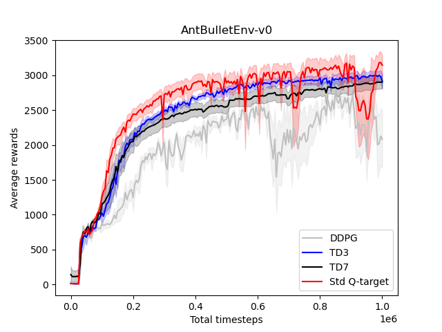
The following plot summarizes the results of SQT when applied on top of TD7 vs. DDPG, TD3, and TD7 on the ant bullet task:

SQT when applied on top of TD7 shows a wide-margin performance advantage over all competitors, especially over TD7 whose performance falls under TD3. We hypothesize that the reason is a scenario when the ant turns over due to a suboptimal action, which finally leads to poor performance on TD7, a scenario which does not occur in SQT, due to its conservative nature.
DDPG exhibits a noticeable performance drawback compared to its counterparts. We posit that this disadvantage is particularly pronounced in risky environments, such as those involving ants that may overturn when the agent undertakes a risky action, resulting in a substantial point loss. This is attributed to DDPG’s inherent problem of overestimation bias, wherein it tends to overvalue suboptimal state-action pairs. Consequently, this overestimation leads to the selection of risky actions, culminating in poor performance. For instance, an ant might overturn or make unfavorable decisions during exploration, adversely affecting overall performance.
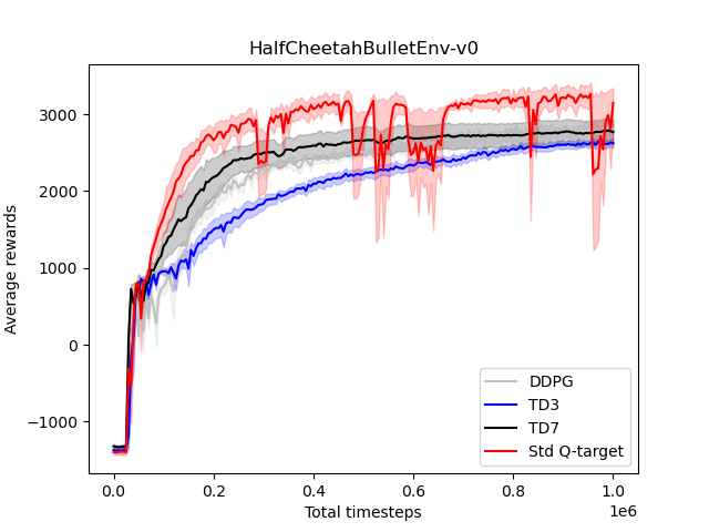
The following plot summarizes the results of SQT when applied on top of TD7 vs. DDPG, TD3, and TD7 on the cheetah bullet task:

SQT when applied on top of TD7 shows a wide-margin performance advantage over all competitors. We hypothesize that the reason is a scenario when the cheetah performs a risky explorative action, i.e. a sharp movement, causing poor data generation and finally a suboptimal performance, a scenario which does not occur in SQT, due to its conservative nature.
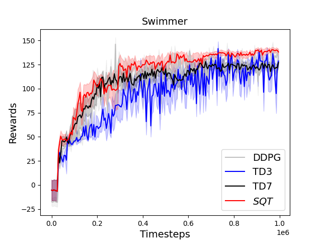
The following plot summarizes the results of SQT when applied on top of TD7 vs. DDPG, TD3, and TD7 on the swimmer task:

SQT when applied on top of TD7 shows a clear performance advantage over all competitors when keeping stable results per-seed. Our hypothesis to SQT’s advantage on the swimmer, is due to the swimmer’s complexity which requires a safe conservative critic’s updates, and punishes for sharp mistaken action, which is a great fit to SQT that uses a conservative critic’s updates. TD3, due to its less conservative updates than SQT’s, can choose poor actions sometimes for exploration, while SQT is more sensitive to poor choices, due to its conservative nature.
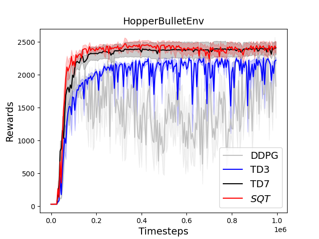
The following plot summarizes the results of SQT when applied on top of TD7 vs. DDPG, TD3, and TD7 on the hopper-bullet task:

SQT when applied on top of TD7 shows a clear performance advantage over all competitors when keeping stable results per-seed. We hypothesize that the reason is a scenario when the hopper performs a risky explorative action, i.e. poor movement, causing the hopper to lose stability and lose performance, a scenario which does not occur in SQT, due to its conservative nature.
TD3 displays a significant level of performance volatility in contrast to SQT. Our conjecture centers around situations where TD3 opts for a risky action, one with a high probability of resulting in poor performance in favor of exploration. This tendency leads to inconsistent results across different seed values, a scenario that does not occur in SQT, as it prioritizes safety over exploration.
In the case of DDPG, there is an evident performance drawback when compared to other models. We theorize that this limitation becomes particularly apparent in environments with instability, such as those involving a hopper that may lose stability when the agent takes a risky action, resulting in a significant loss of points. This is linked to DDPG’s inherent issue of overestimation bias, where it tends to overvalue suboptimal state-action pairs. As a consequence, this tendency to overestimate leads to the selection of risky actions, resulting in subpar performance. For example, a hopper might experience instability or make unfavorable decisions during exploration, negatively impacting overall performance.
5 Related work
-learning’s algorithm can be summarized with the following pseudo-code:
| (8) |
Conservative policy creation (CPI) Kakade and Langford (2002) is an algorithm that finds an approximately optimal policy given access to a restart distribution and an approximate greedy policy chooser using the following conservative policy update rule:
| (9) |
Which precedes a cure for a blow of the overestimation bias problem.
TD3 Fujimoto et al. (2018) is a proven minimalistic solution to DDPG’s Lillicrap et al. (2015) overestimation bias, it just adds another -function, inspired by Double -learning’s ”double estimator” Hasselt (2010), and takes the minimum -network -values as a conservative estimator. Although TD3 has been demonstrated as promising, it solves a problem by introducing another problem which is underestimation bias, resulting in a poor exploration and finally in suboptimal performance.
TD7 Fujimoto et al. (2023) is a simple actor-critic model-free algorithm based on TD3 that can be summarized to one single main component which is SALE (state-action learned-embedding), i.e., TD7 learns an encoding of the transition dynamics of the MDP, , mapping state-action tuple into the state, in the form of state-encoding, , and a state-action encoding, , which uses as an input to the -function, and to the policy , along with the state-action tuple. TD7 demonstrated a clear performance advantage over TD3 when tested on MuJoCo tasks.
Batch-constrained deep -learning (BCQ) Fujimoto et al. (2019) is a conservative RL algorithm that combines the -networks, with the, -networks, resulting in a weighted -target which favors the minimum, as a modest solution to the problem of overestimation bias of DDPG.
BCQ -target formula is:
| (10) |
MaxMin -learning Lan et al. (2020) is an extension of TD3 that introduces a solution to overestimation bias problem on RL algorithms, by accommodating N -functions, allowing flexible control over bias levels—whether it leans toward overestimation or underestimation—determined by the chosen value of .
This contribution holds significant value in two aspects: Firstly, in its generic extension of TD3 to handle -functions (contrasting with TD3’s limitation to two functions). Secondly, it lays out the formal theoretical properties of the MaxMin algorithm, offering a solid theoretical foundation for subsequent algorithms. Specifically, it proves convergence of MaxMin -learning in tabular settings to the optimal -values () and establishes fundamental principles to verify convergence in ensemble RL algorithms, offering a generic framework for broader algorithmic development.
In MaxMin, the -values are estimated using this formula:
Which estimates the -values by selecting the minimum among a set of -networks for the given state-action pair.
Model-based policy optimization (MBPO) Janner et al. (2019) is a simple procedure of using short model-generated rollouts branched from real data, which, surpasses the sample efficiency of prior model-based methods, and matches the asymptotic performance of the best model-free algorithms.
MBPO uses a branched rollout to collect data: starting from the previous policy’s state distribution, , and then taking steps with the new policy, , inspired by Dyna Sutton (1990) (which do a branched rollout with ).
Randomized ensembled double -learning (REDQ) Chen et al. (2021) is a novel deep ensemble RL algorithm, that, formulates a novel -values formula, and, uses an Update-To-Data (UTD) ratio 1.
It is the first model-free algorithm to use a UTD ratio , reaching a competitive sample-complexity performance to MBPO Janner et al. (2019) without a model. REDQ’s -target formula is:
| (11) |
The -pessimistic -learning Gaskett (2003), strikes a balance between the extreme optimism seen in standard -learning and the extreme pessimism of MiniMax -learning Heger (1994) (5). This approach ensures the robustness of safe areas within the state space regarding the chosen action. In this context, the -pessimistic action-values estimate the anticipated value of taking an action, followed by actions that have the highest value with a probability of , or the lowest value with a probability of . When , it mirrors standard -learning, and when , it aligns with the principles of MiniMax -learning Heger (1994).
The -value estimates in -pessimistic -learning are calculated using the following formula:
This equation combines the reward (), discounted future rewards (), and a weighted combination of the maximum and minimum -values, where the weight modifies the variance between the maximum and minimum action values.
- Klima et al. (2019) is a conservative tabular -learning algorithm based on a single -based operator, the robust TD-operator :
Suppose a -learning agent must learn a robust policy against a malicious adversary who could, take over control in the next state, . The value of the next state, , thus depends on who is in control: if the agent is in control, she can choose an optimal action that maximizes expected return; or if the adversary is in control he might aim to minimize the expected return.
MiniMax -learning algorithm is a -learning-based tabular algorithm that optimizes the -function w.r.t. a risk-based criterion of the worst-case discounted average rewards. MiniMax -learning’s Heger (1994) algorithm can be summarized with the following pseudo-code:
6 Conclusion
SQT is a novel -learning-based, model-free, online, on-policy, Actor-Critic, pessimistic algorithm, tackles the problem of overestimation bias of RL algorithms such as DDPG, by using a single, core, simple idea of adding an ”uncertainty penalty” which based on a -networks disagreement, into the -target formula.
We implement SQT on top of TD3/TD7, as an ensemble-based Actor-Critic algorithm, and test it against DDPG, TD3, and TD7, as the state-of-the-art (SOTA) Actor-Critic, model-free, online algorithms, on seven popular MuJoCo and Bullet locomotion tasks, which are: humanoid, walker, ant, swimmer, ant-bullet, cheetah-bullet, and hopper-bullet. Our results show a clear performance advantage to SQT, on a wide margin, in all the tested tasks over DDPG, TD3, and TD7. Demonstrating the superiority of SQT’s conservative -values formula over TD3’s -values formula on those tasks.
In conclusion, our final statement asserts that addressing the issue of overestimation bias in a model-free, online, on-policy, Actor-Critic, ensemble-based algorithm can be achieved by simply diminishing the SQT term in the -target formula. This reduction acts as an ”uncertainty penalty,” yielding a conservative formulation for -values.
References
- Chen et al. [2021] Xinyue Chen, Che Wang, Zijian Zhou, and Keith W. Ross. Randomized ensembled double q-learning: Learning fast without a model. In International Conference on Learning Representations, 2021.
- Coumans and Bai [2016 2021] Erwin Coumans and Yunfei Bai. Pybullet, a python module for physics simulation for games, robotics and machine learning. http://pybullet.org, 2016–2021.
- Fujimoto et al. [2018] Scott Fujimoto, Herke Hoof, and David Meger. Addressing function approximation error in actor-critic methods. In International conference on machine learning, pages 1587–1596. PMLR, 2018.
- Fujimoto et al. [2019] Scott Fujimoto, David Meger, and Doina Precup. Off-policy deep reinforcement learning without exploration. In International conference on machine learning, pages 2052–2062. PMLR, 2019.
- Fujimoto et al. [2023] Scott Fujimoto, Wei-Di Chang, Edward J Smith, Shixiang Shane Gu, Doina Precup, and David Meger. For sale: State-action representation learning for deep reinforcement learning. arXiv preprint arXiv:2306.02451, 2023.
- Gaskett [2003] Chris Gaskett. Reinforcement learning under circumstances beyond its control. 2003.
- Hasselt [2010] Hado Hasselt. Double q-learning. Advances in neural information processing systems, 23, 2010.
- Heger [1994] Matthias Heger. Consideration of risk in reinforcement learning. In Machine Learning Proceedings 1994, pages 105–111. Elsevier, 1994.
- Janner et al. [2019] Michael Janner, Justin Fu, Marvin Zhang, and Sergey Levine. When to trust your model: Model-based policy optimization. Advances in neural information processing systems, 32, 2019.
- Kakade and Langford [2002] Sham Kakade and John Langford. Approximately optimal approximate reinforcement learning. In Proceedings of the Nineteenth International Conference on Machine Learning, pages 267–274, 2002.
- Klima et al. [2019] Richard Klima, Daan Bloembergen, Michael Kaisers, and Karl Tuyls. Robust temporal difference learning for critical domains. arXiv preprint arXiv:1901.08021, 2019.
- Lan et al. [2020] Qingfeng Lan, Yangchen Pan, Alona Fyshe, and Martha White. Maxmin q-learning: Controlling the estimation bias of q-learning. In International Conference on Learning Representations, 2020.
- Lillicrap et al. [2015] Timothy P Lillicrap, Jonathan J Hunt, Alexander Pritzel, Nicolas Heess, Tom Erez, Yuval Tassa, David Silver, and Daan Wierstra. Continuous control with deep reinforcement learning. arXiv preprint arXiv:1509.02971, 2015.
- Silver et al. [2014] David Silver, Guy Lever, Nicolas Heess, Thomas Degris, Daan Wierstra, and Martin Riedmiller. Deterministic policy gradient algorithms. In International conference on machine learning, pages 387–395. Pmlr, 2014.
- Sutton [1990] Richard S Sutton. Integrated architectures for learning, planning, and reacting based on approximating dynamic programming. In Machine learning proceedings 1990, pages 216–224. Elsevier, 1990.
- Todorov et al. [2012] Emanuel Todorov, Tom Erez, and Yuval Tassa. Mujoco: A physics engine for model-based control. In 2012 IEEE/RSJ international conference on intelligent robots and systems, pages 5026–5033. IEEE, 2012.
- Watkins and Dayan [1992] Christopher JCH Watkins and Peter Dayan. Q-learning. Machine learning, 8:279–292, 1992.
- Zhang et al. [2017] Zongzhang Zhang, Zhiyuan Pan, and Mykel J Kochenderfer. Weighted double q-learning. In IJCAI, pages 3455–3461, 2017.