An ADMM-Based Geometric Configuration Optimization in RSSD-Based Source Localization By UAVs with Spread Angle Constraint

Xin Cheng, Weiqiang Zhu, Feng Shu, and Jiangzhou Wang Xin Cheng. Email: xincstar23@163.com. Weiqiang Zhu is with the 8511 Research Institute, China Aerospace Science and Industry Corporation, Nanjing 210007, China. Feng Shu is with the School of Information and Communication Engineering, Hainan University, Haikou, 570228, China and with the School of Electronic and Optical Engineering, Nanjing University of Science and Technology, Nanjing, 210094, China. Jiangzhou Wang is with the School of Engineering, University of Kent, Canterbury CT2 7NT, U.K.
Abstract

Deploying multiple unmanned aerial vehicles (UAVs) to locate a signal-emitting source covers a wide range of military and civilian applications like rescue and target tracking. It is well known that the UAVs-source (sensors-target) geometry, namely geometric configuration, significantly affects the final localization accuracy. This paper focuses on the geometric configuration optimization for received signal strength difference (RSSD)-based passive source localization by drone swarm. Different from prior works, this paper considers a general measuring condition where the spread angle of drone swarm centered on the source is constrained. Subject to this constraint, a geometric configuration optimization problem with the aim of maximizing the determinant of Fisher information matrix (FIM) is formulated. After transforming this problem using matrix theory, an alternating direction method of multipliers (ADMM)-based optimization framework is proposed. To solve the subproblems in this framework, two global optimal solutions based on the Von Neumann matrix trace inequality theorem and majorize-minimize (MM) algorithm are proposed respectively. Finally, the effectiveness as well as the practicality of the proposed ADMM-based optimization algorithm are demonstrated by extensive simulations.

Index Terms:
Source localization, unmanned aerial vehicles, received signal strength difference, geometric configuration optimization, Fisher information matrix, alternating direction method of multipliers, region constraint.

I Introduction

Passive source localization has been applied successfully in many applications including disaster rescue, mobile communication and electronic warfare [1, 2, 3]. Recently, with the fast development of unmanned aerial vehicle (UAV) technology, source localization using UAVs has been popular and widely researched [4, 5, 6, 7]. Compared to traditional sensor carriers like ground vehicles, UAV has the features of small size, fast speed and rapid deployment, thus plays an important role in arduous localization tasks.

Considering the diversity of sensors, there are several types of localization systems, e.g., direction of arrival (DoA) [8], time of arrival (ToA) [9], time difference of arrival (TDoA) [10], received signal strength (RSS) [11] and received signal strength difference (RSSD) [12]. Among these types, the RSS/RSSD-based approach is less sensitive to multi-path interference, thus more suitable for complex localization environment. Moreover, the RSS/RSSD-based approach is cost-effective and easy-operating since it does not require tight synchronization or calibration like others [13]. Although both measure the signal strength, unlike the RSS-based approach, the RSSD-based approach does not require knowing the transmit power of signal-emitting source [14]. Therefore, in some scenarios where the source belongs to a third party or enemy, only the RSSD-based approach is applicable among the two approaches. Due to these advantages, the RSSD-based source localization system by drone swarm is considered in this paper.

A RSSD-based source localization consists of two stages, i.e., measurement and estimation. Extensive researches focus on designing high-precision estimation method. However, as the prerequisite of estimation, measurement also plays an important role in the final localization precision. How to make measurement becomes a worth-exploring problem. It is well known that for any unbiased estimate, the lower bound of its error can be represented by the Cramér-Rao lower bound (CRLB) [15, 16]. And the CRLB is composed of the measurement condition and the geometric configuration. Specifically, the measurement condition includes the wireless propagation environment and the measurement capability of sensor cluster, and the geometric configuration refers to the measuring positional relationship between the sensor cluster and the source. Therefore, in the RSSD-based source localization system by drone swarm, the geometric configuration, namely measuring positions of UAVs, deserves to be optimized [6, 17].

In decades, the geometric configuration optimization of source localization has been researched mainly following three optimization criterions, in which CRLB and Fisher information matrix (FIM) are used as the evaluation standards. These optimization criterions include D-optimality criterion (maximizing the determinant of FIM), A-optimality criterion (minimizing the trace of CRLB) and E-optimality criterion (minimizing the maximum eigenvalue of CRLB). Based on the above criterions, the geometric configuration of RSS-based localization system was optimized in [18, 19, 20]. A closed-form optimal geometric configuration for equal-weight cases where measurement capabilities of different sensor are identical was presented in [18]. Besides, several numerical optimization algorithms were proposed based on frame theory [18], resistive network method [19] and ADMM [20]. Compared to the RSS-based localization, the geometric configuration optimization of RSSD-based localization is more complex due to the unknown transmit power. And it has not been investigated until recent years [21, 22, 23]. In [21], a closed-form optimal geometric configuration was derived for the scenario where three sensors were deployed. In [22], only the equal-weight scenario was considered, the theoretical analysis showed that when the geometric configuration reaches the optimum, the sensors are uniformly distributed on a circle centred on the source. In [23], two suboptimal geometric configuration optimization algorithms were proposed, one was based on gradient descent and the other was based on sequential optimization.

It is worth mentioning that works in [21, 22, 23] have not considered the measuring region constraint. However, due to limitations such as terrain, detection of enemy and communication range, the measuring positions of sensors are often constrained in a practical localization system by UAVs. Certainly, this constraint makes the optimization problem more cumbersome. In recent years, scholars have studied this kind of optimization problem with different region constraints for several types of localization. In [17], the geometric configuration optimization problem with distance constraints between sensors and the source for RSS-based localization was analyzed, and several numerical algorithms based on frame theory were proposed to find the optimal solutions. In [24], any closed measuring region away from the source was considered, and an analytical geometric configuration for AoA localization was derived. For TDoA localization with any measuring region with spread angle less than π2𝜋2\frac{\pi}{2}, an analytical geometric configuration was derived in [25]. In [26], the geometric configuration optimization problem for mixed range/angle/RSS localization was studied while the measuring region was a bow-shaped arch centered on the source, the max values of objective function versus the spread angle of this arch were given out. Moreover it was concluded that the best measurement is reachable when the spread angle is greater than 3π43𝜋4\frac{3\pi}{4}. However, it is hard to extend these works in [17, 24, 25, 26] to the RSSD-based localization system.

To overcome the shortcoming of existing works, in this paper, the geometric configuration optimization of RSSD-based source localization system by drone swarm is studied, and a general constrained measuring region is considered. Specifically, the measuring positions of UAVs are optimized with the spread angle constraint of drone swarm with respect to the source. The major contributions of this paper can be summarized as follows:

  1. 1.

    For the RSSD-based source localization system by drone swarm, considering constrained spread angle of drone swarm, the geometric configuration optimization problem is formulated following the D-optimization criterion. Then the multi-scalar optimization problem is equivalently transformed into a multi-vector optimization problem and a single-matrix optimization problem. These derived problem forms provide valuable insight for the constrained geometric configuration optimization.

  2. 2.

    An ADMM-based constrained geometric configuration optimization algorithm is developed. Specifically, the ADMM framework is introduced to solve the derived single-matrix optimization problem. To solve the two subproblems in ADMM iterations, a closed-form optimal solution and a MM-based optimal algorithm are proposed respectively. Although the proposed algorithm is designed for the RSSD-based localization, it can be also extended easily to other types of localization including RSS, DoA and TDoA.

  3. 3.

    Extensive simulations are conducted for various testing scenarios. The simulation results verify the effectiveness of the proposed algorithm on improving the upper limit of localization precision. Furthermore, considering an initial estimation error in practical scenarios, the practicality of the proposed algorithm on refining the initial estimation is demonstrated.

The rest of this paper is organized as follows. The measuring model is presented and the constrained geometric configuration optimization problem is formulated in Section II. In Section III, the optimization problem is transformed into a vector form and a matrix form. Then an ADMM-based algorithm is proposed in Section IV. In Section V, numerical results are presented. Finally, conclusions are drawn in Section VI.

Notations: Boldface lower case and boldface upper case letters denote vectors and matrices, respectively. Sign ()Tsuperscript𝑇(\cdot)^{T} denotes the transpose operation. ||||||\cdot|| denotes the Frobenius norm of a matrix or the L2 norm of a vector. 𝔼{}𝔼\mathbb{E}\{\cdot\} represents the expectation operation. Tr()Tr\mathrm{Tr}(\cdot) represents the trace of a matrix. |||\cdot| represents the determinant of a matrix. ReRe\mathrm{Re} represents the real part of a number.

II Measurement Model and Problem Form
Refer to caption
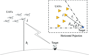
Figure 1: RSSD-based Source Localization via UAVs with Spread Angle Constraint.

II-A Measurement Model

Consider a RSSD-based source localization system by UAVs as shown in Fig. 1, where N𝑁N UAVs are employed to locate a signal-emitting source. The source is located on the ground and emits wireless signal with unknown transmit power. Its position is expressed as 𝐬=[xy0]𝐬matrix𝑥𝑦0\mathbf{s}=\begin{bmatrix}x&y&0\end{bmatrix}. In this localization system, UAVs hovering at different positions receive the wireless signal from the source and measure the strength of it by equipped sensors. Finally, the position of source can be estimated based on these measurements.

In the measurement phase, the position of the i𝑖i-th UAV is expressed as 𝐮i=[xiyizi]subscript𝐮𝑖matrixsubscript𝑥𝑖subscript𝑦𝑖subscript𝑧𝑖\mathbf{u}_{i}=\begin{bmatrix}x_{i}&y_{i}&z_{i}\end{bmatrix}, and the distance between the i𝑖i-th UAV and the target, denoted as disubscript𝑑𝑖d_{i}, is given by

di=(xxi)2+(yyi)2+zi2,i=1,2,,N.formulae-sequencesubscript𝑑𝑖superscript𝑥subscript𝑥𝑖2superscript𝑦subscript𝑦𝑖2superscriptsubscript𝑧𝑖2𝑖12𝑁\displaystyle d_{i}=\sqrt{(x-x_{i})^{2}+(y-y_{i})^{2}+z_{i}^{2}},~{}i=1,2,\cdots,N. (1)

According to the traditional path loss model of wireless propagation (as shown in [11]), the RSS of the i𝑖i-th UAV is expressed as

Pi=P010γlg(di)fi(𝜽)+ηi,i,subscript𝑃𝑖subscriptsubscript𝑃010𝛾lgsubscript𝑑𝑖subscript𝑓𝑖𝜽subscript𝜂𝑖for-all𝑖\displaystyle P_{i}=\underbrace{P_{0}-10\gamma\lg(d_{i})}_{f_{i}(\bm{\theta})}+\eta_{i},~{}\forall i, (2)

where P0subscript𝑃0P_{0} represents the referenced power (in dB form) of source, γ𝛾\gamma is the path loss exponent (PLE), ηisubscript𝜂𝑖\eta_{i} represents the measurement noise following the zero-mean Gaussian distribution with standard deviation σisubscript𝜎𝑖\sigma_{i}, and 𝜽[P0𝐬T]T𝜽superscriptmatrixsubscript𝑃0superscript𝐬𝑇𝑇\bm{\theta}\triangleq\begin{bmatrix}P_{0}&\mathbf{s}^{T}\end{bmatrix}^{T}. The term 𝜽𝜽\bm{\theta} is used to describe all unknown variables in this measurement.

Based on the Eq. (2), all measurements by drone swarm can be represented in a vector form as follows.

𝐏=𝐟(𝜽)+𝜼,𝐏𝐟𝜽𝜼\displaystyle\mathbf{P}=\mathbf{f}(\bm{\theta})+\bm{\eta}, (3)

where 𝐏N×1𝐏superscript𝑁1\mathbf{P}\in\mathbb{R}^{N\times 1} is the vector form of {Pi}i=1Nsuperscriptsubscriptsubscript𝑃𝑖𝑖1𝑁\{P_{i}\}_{i=1}^{N}, 𝐟(𝐬)N×1𝐟𝐬superscript𝑁1\mathbf{f}(\mathbf{s})\in\mathbb{R}^{N\times 1} is the vector form of {fi}i=1Nsuperscriptsubscriptsubscript𝑓𝑖𝑖1𝑁\{f_{i}\}_{i=1}^{N}, and 𝜼N×1𝜼superscript𝑁1\bm{\eta}\in\mathbb{R}^{N\times 1} is the vector form of the {ηi}i=1Nsuperscriptsubscriptsubscript𝜂𝑖𝑖1𝑁\{\eta_{i}\}_{i=1}^{N}. Accordingly, the probability density function (PDF) of 𝜽𝜽\bm{\theta} is given by

Q(𝜽)=1(2π)N2|𝐍|12exp{12(𝐫𝐟(𝜽))T𝐍1(𝐫𝐟(𝜽))}.𝑄𝜽1superscript2𝜋𝑁2superscript𝐍1212superscript𝐫𝐟𝜽𝑇superscript𝐍1𝐫𝐟𝜽\displaystyle Q(\bm{\theta})=\frac{1}{(2\pi)^{\frac{N}{2}}|\mathbf{N}|^{\frac{1}{2}}}\exp\{-\frac{1}{2}(\mathbf{r}-\mathbf{f}(\bm{\theta}))^{T}\mathbf{N}^{-1}(\mathbf{r}-\mathbf{f}(\bm{\theta}))\}. (4)

II-B Problem of Geometric Configuration Optimization

In the estimation phase, following maximum likelihood estimate (MLE), numerical methods can be used to infer the position of source based on the equation (4). We denote an unbiased estimation by 𝐬^^𝐬\mathbf{\hat{s}}, the covariance matrix of its error satisfies the following well-known inequality [15].

𝔼{(𝐬^𝐬)(𝐬^𝐬)T}𝐂=𝐅1.succeeds-or-equals𝔼^𝐬𝐬superscript^𝐬𝐬𝑇𝐂superscript𝐅1\displaystyle\mathbb{E}\left\{(\mathbf{\hat{s}}-\mathbf{s})(\mathbf{\hat{s}}-\mathbf{s})^{T}\right\}\succeq\mathbf{C}=\mathbf{F}^{-1}. (5)

where 𝐂𝐂\mathbf{C} is the CRLB matrix, and 𝐅𝐅\mathbf{F} is the FIM [15] given by

𝐅=𝔼𝜼{𝐬logQ(𝐬)𝐬logQ(𝐬)T}.𝐅subscript𝔼𝜼subscript𝐬𝑄𝐬subscript𝐬𝑄superscript𝐬𝑇\displaystyle\mathbf{F}=\mathbb{E}_{\bm{\eta}}\{\nabla_{\mathbf{s}}\log{Q(\mathbf{s})}\nabla_{\mathbf{s}}\log{Q(\mathbf{s})}^{T}\}. (6)

Eq. (5) implies that 𝐂𝐂\mathbf{C} and 𝐅𝐅\mathbf{F} can be used to guide the measurement of drone swarm. It is well known that the measuring positions of UAVs with respect to the source, namely geometric configuration, are important components of 𝐂𝐂\mathbf{C} or 𝐅𝐅\mathbf{F} [2, 17]. Therefore these measuring positions are optimized in this paper accordingly to improve the measurement quality as well as the final estimation accuracy. Moreover, the D-optimization criterion, i.e., maximizing the determinant of FIM, is applied to guide this optimization. Note that maximizing the determinant of FIM is equivalent to maximizing the amount of information contained in the noisy measurements and minimizing the volume of the uncertainty ellipsoid [16, 26].

To make the geometric configuration optimization concise, we reexpress the measuring positions of UAVs with respect to the source. The horizontal distance between the i𝑖i-th UAV and the source is denoted as risubscript𝑟𝑖r_{i}. The vertical distance between the i𝑖i-th UAV and the source, which is also the flying hight of the i𝑖i-th UAV, is denoted as hisubscript𝑖h_{i}. The horizontal angle of the i𝑖i-th UAV with respect to the source is denoted as βisubscript𝛽𝑖\beta_{i}, i.e., tan(βi)=xixyiysubscript𝛽𝑖subscript𝑥𝑖𝑥subscript𝑦𝑖𝑦\tan(\beta_{i})=\frac{x_{i}-x}{y_{i}-y}. Note that in the three-dimensional space, 𝐮isubscript𝐮𝑖\mathbf{u}_{i} is determined uniquely by risubscript𝑟𝑖r_{i}, hisubscript𝑖h_{i} and βisubscript𝛽𝑖\beta_{i}. Assume the distances between each UAV and the source are fixed 111The optimization of distances between each UAV and the source is straightforward, and independent of the optimization of angles [17].. But the horizontal angles of UAVs are variables to be optimized. Moreover, as shown in Fig. 1, a general constraint is considered where the spread horizontal angle of drone swarm centered on the source is limited, i.e., 0βiβmax,iformulae-sequence0subscript𝛽𝑖subscript𝛽𝑚𝑎𝑥for-all𝑖0\leq\beta_{i}\leq\beta_{max},~{}\forall i.

Following the D-optimization criterion, the geometric configuration optimization problem for the RSSD-based localization system by drone swarm under the above measuring constraint is formulated as

(P1)::P1absent\displaystyle\mathrm{(P1)}: max{βi}i=1N|𝐅|subscriptsuperscriptsubscriptsubscript𝛽𝑖𝑖1𝑁𝐅\displaystyle\max_{\{\beta_{i}\}_{i=1}^{N}}~{}~{}~{}~{}~{}~{}~{}~{}~{}~{}|\mathbf{F}|
s. t.0βiβmax,i.formulae-sequences. t.0subscript𝛽𝑖subscript𝛽𝑚𝑎𝑥for-all𝑖\displaystyle\text{s. t.}~{}~{}~{}~{}~{}0\leq\beta_{i}\leq\beta_{max},~{}\forall i. (7)

III Problem Transformation and Analysis

In this section, the specific expression of FIM is derived. Then the problem (P1)P1\mathrm{(P1)} is transformed into a multi-vector optimization problem by replacing the horizontal angle with a unit directional vector. Based on this, a theorem about equivalent geometric configurations is presented. Finally, the problem is transformed into a concise single-matrix optimization problem by improving the dimension of vectorial variables.

Starting from Eq. (6), FIM is further expressed as

𝐅=[a𝐛T𝐛𝐃],𝐅matrix𝑎superscript𝐛𝑇𝐛𝐃\displaystyle\mathbf{F}=\begin{bmatrix}a&\mathbf{b}^{T}\\ \mathbf{b}&\mathbf{D}\end{bmatrix}, (8a)
a=𝐉T𝐍1𝐉,𝑎superscript𝐉𝑇superscript𝐍1𝐉\displaystyle a=\mathbf{J}^{T}\mathbf{N}^{-1}\mathbf{J}, (8b)
𝐛=[𝐉T𝐍1𝐚x𝐉T𝐍1𝐚y],𝐛matrixsuperscript𝐉𝑇superscript𝐍1subscript𝐚𝑥superscript𝐉𝑇superscript𝐍1subscript𝐚𝑦\displaystyle\mathbf{b}=\begin{bmatrix}\mathbf{J}^{T}\mathbf{N}^{-1}\mathbf{a}_{x}&\mathbf{J}^{T}\mathbf{N}^{-1}\mathbf{a}_{y}\end{bmatrix}, (8c)
𝐃=[𝐚xT𝐍1𝐚x𝐚xT𝐍1𝐚y𝐚xT𝐍1𝐚y𝐚yT𝐍1𝐚y],𝐃matrixsuperscriptsubscript𝐚𝑥𝑇superscript𝐍1subscript𝐚𝑥superscriptsubscript𝐚𝑥𝑇superscript𝐍1subscript𝐚𝑦superscriptsubscript𝐚𝑥𝑇superscript𝐍1subscript𝐚𝑦superscriptsubscript𝐚𝑦𝑇superscript𝐍1subscript𝐚𝑦\displaystyle\mathbf{D}=\begin{bmatrix}\mathbf{a}_{x}^{T}\mathbf{N}^{-1}\mathbf{a}_{x}&\mathbf{a}_{x}^{T}\mathbf{N}^{-1}\mathbf{a}_{y}\\ \mathbf{a}_{x}^{T}\mathbf{N}^{-1}\mathbf{a}_{y}&\mathbf{a}_{y}^{T}\mathbf{N}^{-1}\mathbf{a}_{y}\end{bmatrix}, (8d)

where,

𝐉=[1,1,,1],𝐉111\displaystyle\mathbf{J}=\left[1,1,\cdots,1\right], (9a)
𝐚x=[10γln10x1xd1210γln10x2xd2210γln10xNxdN2],subscript𝐚𝑥matrix10𝛾10subscript𝑥1𝑥superscriptsubscript𝑑1210𝛾10subscript𝑥2𝑥superscriptsubscript𝑑2210𝛾10subscript𝑥𝑁𝑥superscriptsubscript𝑑𝑁2\displaystyle\mathbf{a}_{x}=\begin{bmatrix}\frac{10\gamma}{\ln{10}}\frac{x_{1}-x}{d_{1}^{2}}&\frac{10\gamma}{\ln{10}}\frac{x_{2}-x}{d_{2}^{2}}&\cdots&\frac{10\gamma}{\ln{10}}\frac{x_{N}-x}{d_{N}^{2}}\end{bmatrix}, (9b)
𝐚y=[10γln10y1yd1210γln10y2yd2210γln10yNydN2].subscript𝐚𝑦matrix10𝛾10subscript𝑦1𝑦superscriptsubscript𝑑1210𝛾10subscript𝑦2𝑦superscriptsubscript𝑑2210𝛾10subscript𝑦𝑁𝑦superscriptsubscript𝑑𝑁2\displaystyle\mathbf{a}_{y}=\begin{bmatrix}\frac{10\gamma}{\ln{10}}\frac{y_{1}-y}{d_{1}^{2}}&\frac{10\gamma}{\ln{10}}\frac{y_{2}-y}{d_{2}^{2}}&\cdots&\frac{10\gamma}{\ln{10}}\frac{y_{N}-y}{d_{N}^{2}}\end{bmatrix}. (9c)

To make the expression of FIM more intuitive and analyzable, we define the following symbols.

𝐖tr1(𝐍1)𝐍1,𝐖superscripttr1superscript𝐍1superscript𝐍1\displaystyle\mathbf{W}\triangleq\mathrm{tr}^{-1}(\mathbf{N}^{-1})\mathbf{N}^{-1}, (10a)
σ2¯1Ni=1Nσi2.¯superscript𝜎21𝑁superscriptsubscript𝑖1𝑁superscriptsubscript𝜎𝑖2\displaystyle\overline{\sigma^{-2}}\triangleq\frac{1}{N}\sum_{i=1}^{N}\sigma_{i}^{-2}. (10b)

Based on Eq. (8) and Eq. (10), the objective function of problem (P1)P1\mathrm{(P1)}, i.e., the determinant of FIM is given by

|𝐅|=|a||𝐃𝐛a1𝐛T|=N2σ2¯2|𝐓|,𝐅𝑎𝐃𝐛superscript𝑎1superscript𝐛𝑇superscript𝑁2superscript¯superscript𝜎22superscript𝐓\displaystyle|\mathbf{F}|=|a||\mathbf{D}-\mathbf{b}a^{-1}\mathbf{b}^{T}|=N^{2}\overline{\sigma^{-2}}^{2}|\mathbf{T}^{{}^{\prime}}|, (11)

where,

𝐓superscript𝐓\displaystyle\mathbf{T}^{{}^{\prime}}
=[𝐚xT𝐖𝐚x(𝐚xT𝐖𝐉)2𝐚xT𝐖𝐚y𝐚xT𝐖𝐉𝐚yT𝐖𝐉𝐚xT𝐖𝐚y𝐚xT𝐖𝐉𝐚yT𝐖𝐉𝐚yT𝐖𝐚y(𝐚yT𝐖𝐉)2]absentmatrixsuperscriptsubscript𝐚𝑥𝑇subscript𝐖𝐚𝑥superscriptsuperscriptsubscript𝐚𝑥𝑇𝐖𝐉2superscriptsubscript𝐚𝑥𝑇subscript𝐖𝐚𝑦superscriptsubscript𝐚𝑥𝑇superscriptsubscript𝐖𝐉𝐚𝑦𝑇𝐖𝐉superscriptsubscript𝐚𝑥𝑇subscript𝐖𝐚𝑦superscriptsubscript𝐚𝑥𝑇superscriptsubscript𝐖𝐉𝐚𝑦𝑇𝐖𝐉superscriptsubscript𝐚𝑦𝑇subscript𝐖𝐚𝑦superscriptsuperscriptsubscript𝐚𝑦𝑇𝐖𝐉2\displaystyle=\begin{bmatrix}\mathbf{a}_{x}^{T}\mathbf{W}\mathbf{a}_{x}-(\mathbf{a}_{x}^{T}\mathbf{W}\mathbf{J})^{2}&\mathbf{a}_{x}^{T}\mathbf{W}\mathbf{a}_{y}-\mathbf{a}_{x}^{T}\mathbf{W}\mathbf{J}\mathbf{a}_{y}^{T}\mathbf{W}\mathbf{J}\\ \mathbf{a}_{x}^{T}\mathbf{W}\mathbf{a}_{y}-\mathbf{a}_{x}^{T}\mathbf{W}\mathbf{J}\mathbf{a}_{y}^{T}\mathbf{W}\mathbf{J}&\mathbf{a}_{y}^{T}\mathbf{W}\mathbf{a}_{y}-(\mathbf{a}_{y}^{T}\mathbf{W}\mathbf{J})^{2}\end{bmatrix}
=[𝐚xT(𝐖𝐖𝐉(𝐖𝐉)T)𝐚x𝐚xT(𝐖𝐖𝐉(𝐖𝐉)T)𝐚y𝐚xT(𝐖𝐖𝐉(𝐖𝐉)T)𝐚y𝐚yT(𝐖𝐖𝐉(𝐖𝐉)T)𝐚y]absentmatrixsuperscriptsubscript𝐚𝑥𝑇𝐖𝐖𝐉superscript𝐖𝐉𝑇subscript𝐚𝑥superscriptsubscript𝐚𝑥𝑇𝐖𝐖𝐉superscript𝐖𝐉𝑇subscript𝐚𝑦superscriptsubscript𝐚𝑥𝑇𝐖𝐖𝐉superscript𝐖𝐉𝑇subscript𝐚𝑦superscriptsubscript𝐚𝑦𝑇𝐖𝐖𝐉superscript𝐖𝐉𝑇subscript𝐚𝑦\displaystyle=\begin{bmatrix}\mathbf{a}_{x}^{T}(\mathbf{W}-\mathbf{W}\mathbf{J}(\mathbf{W}\mathbf{J})^{T})\mathbf{a}_{x}&\mathbf{a}_{x}^{T}(\mathbf{W}-\mathbf{W}\mathbf{J}(\mathbf{W}\mathbf{J})^{T})\mathbf{a}_{y}\\ \mathbf{a}_{x}^{T}(\mathbf{W}-\mathbf{W}\mathbf{J}(\mathbf{W}\mathbf{J})^{T})\mathbf{a}_{y}&\mathbf{a}_{y}^{T}(\mathbf{W}-\mathbf{W}\mathbf{J}(\mathbf{W}\mathbf{J})^{T})\mathbf{a}_{y}\end{bmatrix}
=[𝐚xT𝐚yT](𝐖𝐖𝐉(𝐖𝐉)T)[𝐚x𝐚y].absentmatrixsuperscriptsubscript𝐚𝑥𝑇superscriptsubscript𝐚𝑦𝑇𝐖𝐖𝐉superscript𝐖𝐉𝑇matrixsubscript𝐚𝑥subscript𝐚𝑦\displaystyle=\begin{bmatrix}\mathbf{a}_{x}^{T}\\ \mathbf{a}_{y}^{T}\end{bmatrix}(\mathbf{W}-\mathbf{W}\mathbf{J}(\mathbf{W}\mathbf{J})^{T})\begin{bmatrix}\mathbf{a}_{x}&\mathbf{a}_{y}\end{bmatrix}. (12)

Considering the relative position relationship between UAVs and the source as described in Section II, we have

[𝐚xT𝐚yT]isubscriptmatrixsuperscriptsubscript𝐚𝑥𝑇superscriptsubscript𝐚𝑦𝑇𝑖\displaystyle\begin{bmatrix}\mathbf{a}_{x}^{T}\\ \mathbf{a}_{y}^{T}\end{bmatrix}_{i} =[10γln10xixdi210γln10yiydi2]absentmatrix10𝛾10subscript𝑥𝑖𝑥superscriptsubscript𝑑𝑖210𝛾10subscript𝑦𝑖𝑦superscriptsubscript𝑑𝑖2\displaystyle=\begin{bmatrix}\frac{10\gamma}{\ln{10}}\frac{x_{i}-x}{d_{i}^{2}}&\frac{10\gamma}{\ln{10}}\frac{y_{i}-y}{d_{i}^{2}}\end{bmatrix}
=[10γln10ricosβidi210γln10risinβidi2]absentmatrix10𝛾10subscript𝑟𝑖subscript𝛽𝑖superscriptsubscript𝑑𝑖210𝛾10subscript𝑟𝑖subscript𝛽𝑖superscriptsubscript𝑑𝑖2\displaystyle=\begin{bmatrix}\frac{10\gamma}{\ln{10}}\frac{r_{i}\cos{\beta_{i}}}{d_{i}^{2}}&\frac{10\gamma}{\ln{10}}\frac{r_{i}\sin{\beta_{i}}}{d_{i}^{2}}\end{bmatrix}
=10γln10ridi2[cosβisinβi]=10γln10ridi2𝐠i,i,formulae-sequenceabsent10𝛾10subscript𝑟𝑖superscriptsubscript𝑑𝑖2matrixsubscript𝛽𝑖subscript𝛽𝑖10𝛾10subscript𝑟𝑖superscriptsubscript𝑑𝑖2subscript𝐠𝑖for-all𝑖\displaystyle=\frac{10\gamma}{\ln{10}}\frac{r_{i}}{d_{i}^{2}}\begin{bmatrix}\cos{\beta_{i}}&\sin{\beta_{i}}\end{bmatrix}=\frac{10\gamma}{\ln{10}}\frac{r_{i}}{d_{i}^{2}}\mathbf{g}_{i},~{}\forall i, (13)

where [𝐚xT𝐚yT]isubscriptmatrixsuperscriptsubscript𝐚𝑥𝑇superscriptsubscript𝐚𝑦𝑇𝑖\begin{bmatrix}\mathbf{a}_{x}^{T}\\ \mathbf{a}_{y}^{T}\end{bmatrix}_{i} is the i𝑖i-th column of [𝐚xT𝐚yT]matrixsuperscriptsubscript𝐚𝑥𝑇superscriptsubscript𝐚𝑦𝑇\begin{bmatrix}\mathbf{a}_{x}^{T}\\ \mathbf{a}_{y}^{T}\end{bmatrix}, and 𝐠i[cosβisinβi]subscript𝐠𝑖matrixsubscript𝛽𝑖subscript𝛽𝑖\mathbf{g}_{i}\triangleq\begin{bmatrix}\cos{\beta_{i}}&\sin{\beta_{i}}\end{bmatrix}. This defined vector is a unit directional vector, and accounts for the influencing factor to the measuring information amount caused by the horizontal angle of the i𝑖i-th UAV. Moreover, it is easy to verify that there exists a one-one onto mapping between 𝐠isubscript𝐠𝑖\mathbf{g}_{i} and βisubscript𝛽𝑖\beta_{i}, which indicates that it is reasonable to replace {βi}i=1Nsuperscriptsubscriptsubscript𝛽𝑖𝑖1𝑁\{\beta_{i}\}_{i=1}^{N} with {𝐠i}i=1Nsuperscriptsubscriptsubscript𝐠𝑖𝑖1𝑁\{\mathbf{g}_{i}\}_{i=1}^{N} as the optimization variables in problem (P1)P1\mathrm{(P1)}.

Substituting (III) into (III), we have

𝐓=superscript𝐓absent\displaystyle\mathbf{T}^{{}^{\prime}}= (10γln10)2superscript10𝛾102\displaystyle\left(\frac{10\gamma}{\ln{10}}\right)^{2}
(i=1Nwiri2di4𝐠i𝐠iT(i=1Nwiridi2𝐠i)(i=1Nwiridi2𝐠i)T𝐓).subscriptsuperscriptsubscript𝑖1𝑁subscript𝑤𝑖superscriptsubscript𝑟𝑖2superscriptsubscript𝑑𝑖4subscript𝐠𝑖superscriptsubscript𝐠𝑖𝑇superscriptsubscript𝑖1𝑁subscript𝑤𝑖subscript𝑟𝑖superscriptsubscript𝑑𝑖2subscript𝐠𝑖superscriptsuperscriptsubscript𝑖1𝑁subscript𝑤𝑖subscript𝑟𝑖superscriptsubscript𝑑𝑖2subscript𝐠𝑖𝑇𝐓\displaystyle\left(\underbrace{\sum_{i=1}^{N}w_{i}\frac{r_{i}^{2}}{d_{i}^{4}}\mathbf{g}_{i}\mathbf{g}_{i}^{T}-(\sum_{i=1}^{N}w_{i}\frac{r_{i}}{d_{i}^{2}}\mathbf{g}_{i})(\sum_{i=1}^{N}w_{i}\frac{r_{i}}{d_{i}^{2}}\mathbf{g}_{i})^{T}}_{\mathbf{T}}\right). (14)

And the determinant of FIM becomes

|𝐅|=(10γln10)4N2σ2¯2|𝐓|.𝐅superscript10𝛾104superscript𝑁2superscript¯superscript𝜎22𝐓\displaystyle|\mathbf{F}|=\left(\frac{10\gamma}{\ln{10}}\right)^{4}N^{2}\overline{\sigma^{-2}}^{2}|\mathbf{T}|. (15)

From above, the objective function of problem (P1)P1\mathrm{(P1)} can be replaced by |𝐓|𝐓|\mathbf{T}|. Before transforming the problem (P1)P1\mathrm{(P1)}, we give a theorem about the geometric configuration by exploiting the properties of |𝐓|𝐓|\mathbf{T}| as follows.

Theorem 1

Given arbitrary but fixed coefficients {ri}i=1Nsuperscriptsubscriptsubscript𝑟𝑖𝑖1𝑁\{r_{i}\}_{i=1}^{N} and {hi}i=1Nsuperscriptsubscriptsubscript𝑖𝑖1𝑁\{h_{i}\}_{i=1}^{N}, if two geometric configurations can convert to each other only by horizontal overall rotation or horizontal overall reflection with respect to the source, then the corresponding determinants of FIM are equal, namely the two geometric configurations are equivalent.

Proof 1

See Appendix A.

Theorem 1 gives equivalent transformations for an arbitrary geometric configuration. It shows that the solutions of problem (P1)P1\mathrm{(P1)} are not unique. And using these transformations, we can obtain other equivalent solutions from a known one.

To replace {βi}i=1Nsuperscriptsubscriptsubscript𝛽𝑖𝑖1𝑁\{\beta_{i}\}_{i=1}^{N} with {𝐠i}i=1Nsuperscriptsubscriptsubscript𝐠𝑖𝑖1𝑁\{\mathbf{g}_{i}\}_{i=1}^{N} in problem (P1)P1\mathrm{(P1)}, the objective function can be replaced with |𝐓|𝐓|\mathbf{T}| in Eq (III), but the constraints in problem (P1)P1\mathrm{(P1)} still need to be transformed. Based on Theorem 1, the transformation is given by the following theorem.

Theorem 2

In problem (P1)P1\mathrm{(P1)}, 0βiβmax0subscript𝛽𝑖subscript𝛽𝑚𝑎𝑥0\leq\beta_{i}\leq\beta_{max} is equivalent to 𝐠i𝐠0subscript𝐠𝑖subscript𝐠0\mathbf{g}_{i}\geq\mathbf{g}_{0}, where

𝐠0={[cosβmax0],βmaxπ[1cosβmax2],βmax>π.\displaystyle\mathbf{g}_{0}=\left\{\begin{aligned} \begin{bmatrix}\cos{\beta_{max}}&0\end{bmatrix},\quad\beta_{max}\leq\pi\\ \begin{bmatrix}-1&\cos{\frac{\beta_{max}}{2}}\end{bmatrix},\quad\beta_{max}>\pi\\ \end{aligned}\right.. (16)
Proof 2

Consider βmaxπsubscript𝛽𝑚𝑎𝑥𝜋\beta_{max}\leq\pi at first. It shows that cosβicosβmaxsubscript𝛽𝑖subscript𝛽𝑚𝑎𝑥\cos{\beta_{i}}\geq\cos{\beta_{max}} means βi<βmaxβi>2πβmaxsubscript𝛽𝑖expectationsubscript𝛽𝑚𝑎𝑥subscript𝛽𝑖2𝜋subscript𝛽𝑚𝑎𝑥\beta_{i}<\beta_{max}\cup\beta_{i}>2\pi-\beta_{max}, and sinβi0subscript𝛽𝑖0\sin{\beta_{i}}\geq 0 means βiπsubscript𝛽𝑖𝜋\beta_{i}\leq\pi. Therefore, when 𝐠i𝐠0subscript𝐠𝑖subscript𝐠0\mathbf{g}_{i}\geq\mathbf{g}_{0}, βisubscript𝛽𝑖\beta_{i} satisfies 0βiβmax0subscript𝛽𝑖subscript𝛽𝑚𝑎𝑥0\leq\beta_{i}\leq\beta_{max}. Moreover, it is obvious that when 0βiβmax0subscript𝛽𝑖subscript𝛽𝑚𝑎𝑥0\leq\beta_{i}\leq\beta_{max}, 𝐠isubscript𝐠𝑖\mathbf{g}_{i} satisfies 𝐠i𝐠0subscript𝐠𝑖subscript𝐠0\mathbf{g}_{i}\geq\mathbf{g}_{0}. From above, 0βiβmax0subscript𝛽𝑖subscript𝛽𝑚𝑎𝑥0\leq\beta_{i}\leq\beta_{max} is equal to 𝐠i𝐠0subscript𝐠𝑖subscript𝐠0\mathbf{g}_{i}\geq\mathbf{g}_{0} when βmaxπsubscript𝛽𝑚𝑎𝑥𝜋\beta_{max}\leq\pi.

Then consider βmax>πsubscript𝛽𝑚𝑎𝑥𝜋\beta_{max}>\pi. sinβicosβmax2subscript𝛽𝑖subscript𝛽𝑚𝑎𝑥2\sin{\beta_{i}}\geq\cos{\frac{\beta_{max}}{2}} means 0βiπ2+βmax25π2βmax2βi2π0subscript𝛽𝑖𝜋2subscript𝛽𝑚𝑎𝑥25𝜋2subscript𝛽𝑚𝑎𝑥2subscript𝛽𝑖2𝜋0\leq\beta_{i}\leq\frac{\pi}{2}+\frac{\beta_{max}}{2}\cup\frac{5\pi}{2}-\frac{\beta_{max}}{2}\leq\beta_{i}\leq 2\pi. According to Theorem 1, 0βiπ2+βmax25π2βmax2βi2π0subscript𝛽𝑖𝜋2subscript𝛽𝑚𝑎𝑥25𝜋2subscript𝛽𝑚𝑎𝑥2subscript𝛽𝑖2𝜋0\leq\beta_{i}\leq\frac{\pi}{2}+\frac{\beta_{max}}{2}\cup\frac{5\pi}{2}-\frac{\beta_{max}}{2}\leq\beta_{i}\leq 2\pi is equivalent to 0βiβmax0subscript𝛽𝑖subscript𝛽𝑚𝑎𝑥0\leq\beta_{i}\leq\beta_{max} in problem (P1)P1\mathrm{(P1)}. Therefore when 𝐠i𝐠0subscript𝐠𝑖subscript𝐠0\mathbf{g}_{i}\geq\mathbf{g}_{0}, βisubscript𝛽𝑖\beta_{i} satisfies 0βiβmax0subscript𝛽𝑖subscript𝛽𝑚𝑎𝑥0\leq\beta_{i}\leq\beta_{max}. Moreover, it is obvious that when 0βiβmax0subscript𝛽𝑖subscript𝛽𝑚𝑎𝑥0\leq\beta_{i}\leq\beta_{max}, 𝐠isubscript𝐠𝑖\mathbf{g}_{i} satisfies 𝐠i𝐠0subscript𝐠𝑖subscript𝐠0\mathbf{g}_{i}\geq\mathbf{g}_{0}. From above, 0βiβmax0subscript𝛽𝑖subscript𝛽𝑚𝑎𝑥0\leq\beta_{i}\leq\beta_{max} is equal to 𝐠i𝐠0subscript𝐠𝑖subscript𝐠0\mathbf{g}_{i}\geq\mathbf{g}_{0} when βmax>πsubscript𝛽𝑚𝑎𝑥𝜋\beta_{max}>\pi.

According to Eq (III), Eq (15) and Theorem 2, problem (P1)P1\mathrm{(P1)} is equivalently transformed into

(P2)::P2absent\displaystyle\mathrm{(P2)}: max{𝐠i}i=1N|𝐓|subscriptsuperscriptsubscriptsubscript𝐠𝑖𝑖1𝑁𝐓\displaystyle\max_{\{\mathbf{g}_{i}\}_{i=1}^{N}}~{}~{}~{}~{}~{}~{}~{}~{}~{}~{}\left|\mathbf{T}\right|
s. t.𝐠iT𝐠i=1,s. t.superscriptsubscript𝐠𝑖𝑇subscript𝐠𝑖1\displaystyle~{}~{}\text{s. t.}~{}~{}~{}~{}~{}~{}~{}~{}~{}~{}\mathbf{g}_{i}^{T}\mathbf{g}_{i}=1,
𝐠i𝐠0,i.subscript𝐠𝑖subscript𝐠0for-all𝑖\displaystyle~{}~{}~{}~{}~{}~{}~{}~{}~{}~{}~{}~{}~{}~{}\mathbf{g}_{i}\geq\mathbf{g}_{0},~{}\forall i. (17)

Although problem (P2)P2\mathrm{(P2)} is more concise than problem (P1)P1\mathrm{(P1)}, it is still intractable due to the coupling of variables associated with different UAVs. Therefore, we continue transform problem (P2)P2\mathrm{(P2)}. At first, we define a new matrix that collects all variables in problem (P2)P2\mathrm{(P2)} as follows.

𝐆[𝐠1T𝐠2T𝐠NT].𝐆matrixsuperscriptsubscript𝐠1𝑇superscriptsubscript𝐠2𝑇superscriptsubscript𝐠𝑁𝑇\displaystyle\mathbf{G}\triangleq\begin{bmatrix}\mathbf{g}_{1}^{T}&\mathbf{g}_{2}^{T}&\cdots&\mathbf{g}_{N}^{T}\end{bmatrix}. (18)

Besides, we define the following matrixes.

𝐃diag([r1d12r2d22rNdN2]),𝐃diagmatrixsubscript𝑟1superscriptsubscript𝑑12subscript𝑟2superscriptsubscript𝑑22subscript𝑟𝑁superscriptsubscript𝑑𝑁2\displaystyle\mathbf{D}\triangleq\mathrm{diag}\left(\begin{bmatrix}\frac{r_{1}}{d_{1}^{2}}&\frac{r_{2}}{d_{2}^{2}}&\cdots&\frac{r_{N}}{d_{N}^{2}}\end{bmatrix}\right), (19)
𝐁𝐖𝐖𝐉(𝐖𝐉)T.𝐁𝐖𝐖𝐉superscript𝐖𝐉𝑇\displaystyle\mathbf{B}\triangleq\mathbf{W}-\mathbf{W}\mathbf{J}(\mathbf{W}\mathbf{J})^{T}. (20)

Based on these definitions, 𝐓𝐓\mathbf{T} in the objective function of problem (P2)P2\mathrm{(P2)} is rewritten as

𝐓𝐓\displaystyle\mathbf{T} =(ln1010γ)4absentsuperscript1010𝛾4\displaystyle=\left(\frac{\ln{10}}{10\gamma}\right)^{4}
[𝐚xT(𝐖𝐖𝐉(𝐖𝐉)T)𝐚x𝐚xT(𝐖𝐖𝐉(𝐖𝐉)T)𝐚y𝐚xT(𝐖𝐖𝐉(𝐖𝐉)T)𝐚y𝐚yT(𝐖𝐖𝐉(𝐖𝐉)T)𝐚y]matrixsuperscriptsubscript𝐚𝑥𝑇𝐖𝐖𝐉superscript𝐖𝐉𝑇subscript𝐚𝑥superscriptsubscript𝐚𝑥𝑇𝐖𝐖𝐉superscript𝐖𝐉𝑇subscript𝐚𝑦superscriptsubscript𝐚𝑥𝑇𝐖𝐖𝐉superscript𝐖𝐉𝑇subscript𝐚𝑦superscriptsubscript𝐚𝑦𝑇𝐖𝐖𝐉superscript𝐖𝐉𝑇subscript𝐚𝑦\displaystyle~{}\begin{bmatrix}\mathbf{a}_{x}^{T}(\mathbf{W}-\mathbf{W}\mathbf{J}(\mathbf{W}\mathbf{J})^{T})\mathbf{a}_{x}&\mathbf{a}_{x}^{T}(\mathbf{W}-\mathbf{W}\mathbf{J}(\mathbf{W}\mathbf{J})^{T})\mathbf{a}_{y}\\ \mathbf{a}_{x}^{T}(\mathbf{W}-\mathbf{W}\mathbf{J}(\mathbf{W}\mathbf{J})^{T})\mathbf{a}_{y}&\mathbf{a}_{y}^{T}(\mathbf{W}-\mathbf{W}\mathbf{J}(\mathbf{W}\mathbf{J})^{T})\mathbf{a}_{y}\end{bmatrix}
=(ln1010γ)4[𝐚xT𝐚yT]𝐁[𝐚x𝐚y]absentsuperscript1010𝛾4matrixsuperscriptsubscript𝐚𝑥𝑇superscriptsubscript𝐚𝑦𝑇𝐁matrixsubscript𝐚𝑥subscript𝐚𝑦\displaystyle=\left(\frac{\ln{10}}{10\gamma}\right)^{4}\begin{bmatrix}\mathbf{a}_{x}^{T}\\ \mathbf{a}_{y}^{T}\end{bmatrix}\mathbf{B}\begin{bmatrix}\mathbf{a}_{x}&\mathbf{a}_{y}\end{bmatrix}
=𝐆T𝐃T𝐁𝐃𝐆.absentsuperscript𝐆𝑇superscript𝐃𝑇𝐁𝐃𝐆\displaystyle=\mathbf{G}^{T}\mathbf{D}^{T}\mathbf{B}\mathbf{D}\mathbf{G}. (21)

For an arbitrary vector 𝝃𝝃\bm{\xi} in Nsuperscript𝑁\mathbb{R}^{N}, the following formula is satisfied.

𝝃T𝐁𝝃superscript𝝃𝑇𝐁𝝃\displaystyle\bm{\xi}^{T}\mathbf{B}\bm{\xi} =𝝃T𝐖𝝃(𝝃T𝐖𝐉)2absentsuperscript𝝃𝑇𝐖𝝃superscriptsuperscript𝝃𝑇𝐖𝐉2\displaystyle=\bm{\xi}^{T}\mathbf{W}\bm{\xi}-(\bm{\xi}^{T}\mathbf{W}\mathbf{J})^{2}
=i=1Nw(i)𝝃2(i)(i=1Kw(i)𝝃(i))2absentsuperscriptsubscript𝑖1𝑁𝑤𝑖superscript𝝃2𝑖superscriptsuperscriptsubscript𝑖1𝐾𝑤𝑖𝝃𝑖2\displaystyle=\sum_{i=1}^{N}w(i)\bm{\xi}^{2}(i)-(\sum_{i=1}^{K}w(i)\bm{\xi}(i))^{2}
=i=1Nw(i)g(𝝃(i))g(i=1Kw(i)𝝃(i))0,absentsuperscriptsubscript𝑖1𝑁𝑤𝑖𝑔𝝃𝑖𝑔superscriptsubscript𝑖1𝐾𝑤𝑖𝝃𝑖0\displaystyle=\sum_{i=1}^{N}w(i)g(\bm{\xi}(i))-g(\sum_{i=1}^{K}w(i)\bm{\xi}(i))\geq 0, (22)

where, g(x)=x2,x𝑔𝑥superscript𝑥2for-all𝑥g(x)=x^{2},~{}\forall x, w(i)𝑤𝑖w(i) is the i𝑖i-th diagonal element of 𝐖𝐖\mathbf{W}. It is easy to verify that w(i)>0,i𝑤𝑖0for-all𝑖w(i)>0,~{}\forall i and i=1Nw(i)=1superscriptsubscript𝑖1𝑁𝑤𝑖1\sum_{i=1}^{N}w(i)=1. The last inequality in formula (III) results from Jensen’s inequality [27]. According to formula (III), 𝐁𝐁\mathbf{B} is a semi-positive definite matrix, thus 𝐁𝐁\mathbf{B} is feasible for the cholesky decomposition, i.e., 𝐁=𝐁12𝐁12T𝐁superscript𝐁12superscript𝐁12𝑇\mathbf{B}=\mathbf{B}^{\frac{1}{2}}\mathbf{B}^{\frac{1}{2}T}. Defining a matrix 𝐗𝐗\mathbf{X} that 𝐗𝐁12𝐃𝐆𝐗superscript𝐁12𝐃𝐆\mathbf{X}\triangleq\mathbf{B}^{\frac{1}{2}}\mathbf{D}\mathbf{G} yields 𝐓=𝐗T𝐗𝐓superscript𝐗𝑇𝐗\mathbf{T}=\mathbf{X}^{T}\mathbf{X}. Finally, problem (P2)P2\mathrm{(P2)} is transformed into the following problem.

(P3)::P3absent\displaystyle\mathrm{(P3)}: min𝐆ln|(𝐗T𝐗)1|subscript𝐆superscriptsuperscript𝐗𝑇𝐗1\displaystyle\min_{\mathbf{G}}~{}~{}\ln{\left|(\mathbf{X}^{T}\mathbf{X})^{-1}\right|}
s. t.𝐗=𝐁12𝐃𝐆,s. t.𝐗superscript𝐁12𝐃𝐆\displaystyle\text{s. t.}~{}~{}~{}\mathbf{X}=\mathbf{B}^{\frac{1}{2}}\mathbf{D}\mathbf{G},
𝐆𝒟,𝐆𝒟\displaystyle~{}~{}~{}~{}~{}~{}~{}~{}~{}~{}~{}\mathbf{G}\in\mathcal{D}, (23)

where 𝒟={𝐆|𝐠iT𝐠i=1,𝐠i𝐠0,i}𝒟conditional-set𝐆formulae-sequencesuperscriptsubscript𝐠𝑖𝑇subscript𝐠𝑖1subscript𝐠𝑖subscript𝐠0for-all𝑖\mathcal{D}=\{\mathbf{G}|\mathbf{g}_{i}^{T}\mathbf{g}_{i}=1,~{}\mathbf{g}_{i}\geq\mathbf{g}_{0},~{}\forall i\}.

IV ADMM-Based Constrained Geometric Configuration Optimization Algorithm

IV-A Framework of ADMM

To tackle problem (P3)P3\mathrm{(P3)}, ADMM framework is introduced in this section. Note that ADMM is powerful and widely-used in the matrix optimization problem. It takes the form of a decomposition-coordination procedure, in which the solutions to small local subproblems are coordinated to find a solution to a large global problem [28]. And it blends the benefits of dual decomposition and augmented Lagrangian methods.

At first, we introduce Lagrangian multiplier denoted as 𝐕𝐕\mathbf{V} and augmented Lagrangian parameter denoted as ρ𝜌\rho. Then the augmented Lagrangian of problem (P3)P3\mathrm{(P3)} is expressed as

Lρ(𝐗,𝐆,𝐕)=subscript𝐿𝜌𝐗𝐆𝐕absent\displaystyle L_{\rho}(\mathbf{X},\mathbf{G},\mathbf{V})= ln|(𝐗T𝐗)1|+Tr(𝐕T(𝐁12𝐃𝐆𝐗))superscriptsuperscript𝐗𝑇𝐗1Trsuperscript𝐕𝑇superscript𝐁12𝐃𝐆𝐗\displaystyle\ln{\left|(\mathbf{X}^{T}\mathbf{X})^{-1}\right|}+\mathrm{Tr}\left(\mathbf{V}^{T}(\mathbf{B}^{\frac{1}{2}}\mathbf{D}\mathbf{G}-\mathbf{X})\right)
+ρ2𝐁12𝐃𝐆𝐗2.𝜌2superscriptnormsuperscript𝐁12𝐃𝐆𝐗2\displaystyle+\frac{\rho}{2}\|\mathbf{B}^{\frac{1}{2}}\mathbf{D}\mathbf{G}-\mathbf{X}\|^{2}. (24)

According to [28], the ADMM update framework to solve problem (P3)P3\mathrm{(P3)} is given by

𝐗k+1=argmin𝐗Lρ(𝐗,𝐆k,𝐕k),superscript𝐗𝑘1subscriptargmin𝐗subscript𝐿𝜌𝐗superscript𝐆𝑘superscript𝐕𝑘\displaystyle\mathbf{X}^{k+1}=\mathop{\mathrm{argmin}}_{\mathbf{X}}L_{\rho}(\mathbf{X},\mathbf{G}^{k},\mathbf{V}^{k}), (25a)
𝐆k+1=argmin𝐆𝒟Lρ(𝐗k+1,𝐆,𝐕k),superscript𝐆𝑘1subscriptargmin𝐆𝒟subscript𝐿𝜌superscript𝐗𝑘1𝐆superscript𝐕𝑘\displaystyle\mathbf{G}^{k+1}=\mathop{\mathrm{argmin}}_{\mathbf{G}\in\mathcal{D}}L_{\rho}(\mathbf{X}^{k+1},\mathbf{G},\mathbf{V}^{k}), (25b)
𝐕k+1=𝐕k+ρ(𝐁12𝐃𝐆k+1𝐗k+1),superscript𝐕𝑘1superscript𝐕𝑘𝜌superscript𝐁12superscript𝐃𝐆𝑘1superscript𝐗𝑘1\displaystyle\mathbf{V}^{k+1}=\mathbf{V}^{k}+\rho(\mathbf{B}^{\frac{1}{2}}\mathbf{D}\mathbf{G}^{k+1}-\mathbf{X}^{k+1}), (25c)

where k𝑘k is the iteration number. In this framework, the update of 𝐕𝐕\mathbf{V} is straightforward, but the updates of 𝐗𝐗\mathbf{X} and 𝐆𝐆\mathbf{G} are not. We will given these updates by finding the global optimal solutions of subproblem (25a) and subproblem (25b) in the following subsections.

IV-B Update of 𝐗𝐗\mathbf{X}

At the (k+1)𝑘1(k+1)-th iteration, when 𝐆ksuperscript𝐆𝑘\mathbf{G}^{k} and 𝐕ksuperscript𝐕𝑘\mathbf{V}^{k} are given, Lρ(𝐗,𝐆k,𝐕k)subscript𝐿𝜌𝐗superscript𝐆𝑘superscript𝐕𝑘L_{\rho}(\mathbf{X},\mathbf{G}^{k},\mathbf{V}^{k}) (simplified as Lρksuperscriptsubscript𝐿𝜌𝑘L_{\rho}^{k} in this subsection) in subproblem (25a) can be written as

Lρk=ln|(𝐗T𝐗)1|+ρ2Tr(𝐗T𝐗)Tr(𝐉kT𝐗)+βk,superscriptsubscript𝐿𝜌𝑘superscriptsuperscript𝐗𝑇𝐗1𝜌2Trsuperscript𝐗𝑇𝐗Trsuperscript𝐉𝑘𝑇𝐗superscript𝛽𝑘\displaystyle L_{\rho}^{k}=\ln{\left|(\mathbf{X}^{T}\mathbf{X})^{-1}\right|}+\frac{\rho}{2}\mathrm{Tr}(\mathbf{X}^{T}\mathbf{X})-\mathrm{Tr}\left(\mathbf{J}^{kT}\mathbf{X}\right)+\beta^{k}, (26)

where 𝐉k=𝐕k+ρ𝐁12𝐃𝐆ksuperscript𝐉𝑘superscript𝐕𝑘𝜌superscript𝐁12superscript𝐃𝐆𝑘\mathbf{J}^{k}=\mathbf{V}^{k}+\rho\mathbf{B}^{\frac{1}{2}}\mathbf{D}\mathbf{G}^{k}, βk=𝐓𝐫(𝐕kT𝐁12𝐃𝐆k)+ρ2Tr((𝐁12𝐃𝐆k)T(𝐁12𝐃𝐆k))superscript𝛽𝑘𝐓𝐫superscript𝐕𝑘𝑇superscript𝐁12superscript𝐃𝐆𝑘𝜌2Trsuperscriptsuperscript𝐁12superscript𝐃𝐆𝑘𝑇superscript𝐁12superscript𝐃𝐆𝑘\beta^{k}=\mathbf{Tr}(\mathbf{V}^{kT}\mathbf{B}^{\frac{1}{2}}\mathbf{D}\mathbf{G}^{k})+\frac{\rho}{2}\mathrm{Tr}\left((\mathbf{B}^{\frac{1}{2}}\mathbf{D}\mathbf{G}^{k})^{T}(\mathbf{B}^{\frac{1}{2}}\mathbf{D}\mathbf{G}^{k})\right).

To address subproblem (25a), singular value decomposition (SVD) is applied. Since 𝐗N×2𝐗superscript𝑁2\mathbf{X}\in\mathbb{R}^{N\times 2} and 𝐉kN×2superscript𝐉𝑘superscript𝑁2\mathbf{J}^{k}\in\mathbb{R}^{N\times 2}, the SVDs are expressed as

𝐗=𝐔[𝚲𝟎]𝐕,𝐗𝐔matrix𝚲0𝐕\displaystyle\mathbf{X}=\mathbf{U}\begin{bmatrix}\mathbf{\Lambda}&\mathbf{0}\end{bmatrix}\mathbf{V}, (27)
𝐉k=𝐔Jk[𝚺k𝟎]𝐕Jk,superscript𝐉𝑘superscriptsubscript𝐔𝐽𝑘matrixsuperscript𝚺𝑘0superscriptsubscript𝐕𝐽𝑘\displaystyle\mathbf{J}^{k}=\mathbf{U}_{J}^{k}\begin{bmatrix}\mathbf{\Sigma}^{k}&\mathbf{0}\end{bmatrix}\mathbf{V}_{J}^{k}, (28)

where 𝟎(N2)×20superscript𝑁22\mathbf{0}\in\mathbb{R}^{(N-2)\times 2}, 𝚲=diag([τ1τ2])𝚲diagmatrixsubscript𝜏1subscript𝜏2\mathbf{\Lambda}=\mathrm{diag}\left(\begin{bmatrix}\tau_{1}&\tau_{2}\end{bmatrix}\right) with τ1τ20subscript𝜏1subscript𝜏20\tau_{1}\geq\tau_{2}\geq 0 and 𝚺k=diag([σ1kσ2k])superscript𝚺𝑘diagmatrixsubscriptsuperscript𝜎𝑘1subscriptsuperscript𝜎𝑘2\mathbf{\Sigma}^{k}=\mathrm{diag}\left(\begin{bmatrix}\sigma^{k}_{1}&\sigma^{k}_{2}\end{bmatrix}\right) with σ1kσ2k0subscriptsuperscript𝜎𝑘1subscriptsuperscript𝜎𝑘20\sigma^{k}_{1}\geq\sigma^{k}_{2}\geq 0. Note that {τi}i=12superscriptsubscriptsubscript𝜏𝑖𝑖12\{\tau_{i}\}_{i=1}^{2} are the non-zero singular values of 𝐗𝐗\mathbf{X} and {σik}i=12superscriptsubscriptsubscriptsuperscript𝜎𝑘𝑖𝑖12\{\sigma^{k}_{i}\}_{i=1}^{2} are the non-zero singular values of 𝐉ksuperscript𝐉𝑘\mathbf{J}^{k}. After substituting equation (27) and equation (28) into equation(26), the objective function of subproblem (25a) becomes

Lρk=ln|(𝚲T𝚲)1|+ρ2Tr(𝚲T𝚲)Tr(𝐉kT𝐗)+βk.superscriptsubscript𝐿𝜌𝑘superscriptsuperscript𝚲𝑇𝚲1𝜌2Trsuperscript𝚲𝑇𝚲Trsuperscript𝐉𝑘𝑇𝐗superscript𝛽𝑘\displaystyle L_{\rho}^{k}=\ln{\left|(\mathbf{\Lambda}^{T}\mathbf{\Lambda})^{-1}\right|}+\frac{\rho}{2}\mathrm{Tr}(\mathbf{\Lambda}^{T}\mathbf{\Lambda})-\mathrm{Tr}\left(\mathbf{J}^{kT}\mathbf{X}\right)+\beta^{k}. (29)

According to Theorem 1 in [29], which is a corollary of the Von Neumann’s trace inequality [30], we have

Tr(𝐉kT𝐗)i=12|Reλi(𝐓~)|τiσik,Trsuperscript𝐉𝑘𝑇𝐗superscriptsubscript𝑖12Resubscript𝜆𝑖~𝐓subscript𝜏𝑖subscriptsuperscript𝜎𝑘𝑖\displaystyle\mathrm{Tr}\left(\mathbf{J}^{kT}\mathbf{X}\right)\leq\sum_{i=1}^{2}|\mathrm{Re}\lambda_{i}(\tilde{\mathbf{T}})|\tau_{i}\sigma^{k}_{i}, (30)

where,

𝐓~=𝐔JkT𝐔[𝐕𝐕JkT𝟎𝟎𝐈N2],~𝐓superscriptsubscript𝐔𝐽𝑘𝑇𝐔matrixsuperscriptsubscript𝐕𝐕𝐽𝑘𝑇00subscript𝐈𝑁2\displaystyle\tilde{\mathbf{T}}=\mathbf{U}_{J}^{kT}\mathbf{U}\begin{bmatrix}\mathbf{V}\mathbf{V}_{J}^{kT}&\mathbf{0}\\ \mathbf{0}&\mathbf{I}_{N-2}\end{bmatrix}, (31)

where λi(𝐓~)subscript𝜆𝑖~𝐓\lambda_{i}(\tilde{\mathbf{T}}) denotes the i𝑖i-th eigenvalue of 𝐓~~𝐓\tilde{\mathbf{T}} with λi1(𝐓~)>λi(𝐓~)subscript𝜆𝑖1~𝐓subscript𝜆𝑖~𝐓\lambda_{i-1}(\tilde{\mathbf{T}})>\lambda_{i}(\tilde{\mathbf{T}}).

Because 𝐓~T𝐓~=𝐓~𝐓~T=𝐈Nsuperscript~𝐓𝑇~𝐓~𝐓superscript~𝐓𝑇subscript𝐈𝑁\tilde{\mathbf{T}}^{T}\tilde{\mathbf{T}}=\tilde{\mathbf{T}}\tilde{\mathbf{T}}^{T}=\mathbf{I}_{N}, 𝐓~~𝐓\tilde{\mathbf{T}} is an unitary matrix with |Reλi(𝐓~)|1Resubscript𝜆𝑖~𝐓1|\mathrm{Re}\lambda_{i}(\tilde{\mathbf{T}})|\leq 1. Then we have,

Tr(𝐉kT𝐗)i=12τiσik.Trsuperscript𝐉𝑘𝑇𝐗superscriptsubscript𝑖12subscript𝜏𝑖subscriptsuperscript𝜎𝑘𝑖\displaystyle\mathrm{Tr}\left(\mathbf{J}^{kT}\mathbf{X}\right)\leq\sum_{i=1}^{2}\tau_{i}\sigma^{k}_{i}. (32)

It is easy to verify that when 𝐔=𝐔Jk𝐔superscriptsubscript𝐔𝐽𝑘\mathbf{U}=\mathbf{U}_{J}^{k} and 𝐕=𝐕Jk𝐕superscriptsubscript𝐕𝐽𝑘\mathbf{V}=\mathbf{V}_{J}^{k}, the equation in formula (32) holds, which indicates Lρksuperscriptsubscript𝐿𝜌𝑘L_{\rho}^{k} reaches the minimum. Under this condition,

Lρk=ln|(𝚲T𝚲)1|+ρ2Tr(𝚲T𝚲)Tr(𝚺k𝚲)+βk.superscriptsubscript𝐿𝜌𝑘superscriptsuperscript𝚲𝑇𝚲1𝜌2Trsuperscript𝚲𝑇𝚲Trsuperscript𝚺𝑘𝚲superscript𝛽𝑘\displaystyle L_{\rho}^{k}=\ln{\left|(\mathbf{\Lambda}^{T}\mathbf{\Lambda})^{-1}\right|}+\frac{\rho}{2}\mathrm{Tr}(\mathbf{\Lambda}^{T}\mathbf{\Lambda})-\mathrm{Tr}\left(\mathbf{\Sigma}^{k}\mathbf{\Lambda}\right)+\beta^{k}. (33)

Thereby, Lρksuperscriptsubscript𝐿𝜌𝑘L_{\rho}^{k} has transformed as a function of {λi}i=12superscriptsubscriptsubscript𝜆𝑖𝑖12\{\lambda_{i}\}_{i=1}^{2}. It is straightforward that the minimum of Lρksuperscriptsubscript𝐿𝜌𝑘L_{\rho}^{k} satisfies the following equation.

Lρk=2𝚲1+ρ𝚲𝚺k=𝟎.superscriptsubscript𝐿𝜌𝑘2superscript𝚲1𝜌𝚲superscript𝚺𝑘0\displaystyle\nabla L_{\rho}^{k}=-2\mathbf{\Lambda}^{-1}+\rho\mathbf{\Lambda}-\mathbf{\Sigma}^{k}=\mathbf{0}. (34)

Due to the positive property of λisubscript𝜆𝑖\lambda_{i}, it shows that when Lρksuperscriptsubscript𝐿𝜌𝑘L_{\rho}^{k} reaches the minimum,

λi=σik+(σik)2+8ρ2ρ,i=1,2.formulae-sequencesubscript𝜆𝑖subscriptsuperscript𝜎𝑘𝑖superscriptsubscriptsuperscript𝜎𝑘𝑖28𝜌2𝜌𝑖12\displaystyle\lambda_{i}=\frac{\sigma^{k}_{i}+\sqrt{(\sigma^{k}_{i})^{2}+8\rho}}{2\rho},~{}i=1,2. (35)

From above, the update of 𝐗𝐗\mathbf{X} at the (k+1)𝑘1(k+1)-th iteration is given by

𝐗k+1=𝐔Jk[𝚲k𝟎]𝐕Jk,superscript𝐗𝑘1superscriptsubscript𝐔𝐽𝑘matrixsuperscript𝚲𝑘0superscriptsubscript𝐕𝐽𝑘\displaystyle\mathbf{X}^{k+1}=\mathbf{U}_{J}^{k}\begin{bmatrix}\mathbf{\Lambda}^{k}&\mathbf{0}\end{bmatrix}\mathbf{V}_{J}^{k}, (36)

where 𝚲k=diag([σ1k+(σ1k)2+8ρ2ρσ2k+(σ2k)2+8ρ2ρ])superscript𝚲𝑘diagmatrixsubscriptsuperscript𝜎𝑘1superscriptsubscriptsuperscript𝜎𝑘128𝜌2𝜌subscriptsuperscript𝜎𝑘2superscriptsubscriptsuperscript𝜎𝑘228𝜌2𝜌\mathbf{\Lambda}^{k}=\mathrm{diag}\left(\begin{bmatrix}\frac{\sigma^{k}_{1}+\sqrt{(\sigma^{k}_{1})^{2}+8\rho}}{2\rho}&\frac{\sigma^{k}_{2}+\sqrt{(\sigma^{k}_{2})^{2}+8\rho}}{2\rho}\end{bmatrix}\right).

IV-C Update of 𝐆𝐆\mathbf{G}

At the (k+1)𝑘1(k+1)-th iteration, when 𝐗k+1superscript𝐗𝑘1\mathbf{X}^{k+1} and 𝐕ksuperscript𝐕𝑘\mathbf{V}^{k} are given, Lρ(𝐗k+1,𝐆,𝐕k)subscript𝐿𝜌superscript𝐗𝑘1𝐆superscript𝐕𝑘L_{\rho}(\mathbf{X}^{k+1},\mathbf{G},\mathbf{V}^{k}) (simplified as Lρksuperscriptsubscript𝐿𝜌𝑘L_{\rho}^{k} in this subsection) in subproblem (25b) can be written as

Lρksuperscriptsubscript𝐿𝜌𝑘\displaystyle L_{\rho}^{k}
=ln|(𝐗(k+1)T𝐗k+1)1|+Tr(𝐕kT(𝐁12𝐃𝐆𝐗k+1))absentsuperscriptsuperscript𝐗𝑘1𝑇superscript𝐗𝑘11Trsuperscript𝐕𝑘𝑇superscript𝐁12𝐃𝐆superscript𝐗𝑘1\displaystyle=\ln{\left|(\mathbf{X}^{(k+1)T}\mathbf{X}^{k+1})^{-1}\right|}+\mathrm{Tr}\left(\mathbf{V}^{kT}(\mathbf{B}^{\frac{1}{2}}\mathbf{D}\mathbf{G}-\mathbf{X}^{k+1})\right)
+ρ2𝐁12𝐃𝐆𝐗k+12𝜌2superscriptnormsuperscript𝐁12𝐃𝐆superscript𝐗𝑘12\displaystyle~{}~{}~{}+\frac{\rho}{2}\|\mathbf{B}^{\frac{1}{2}}\mathbf{D}\mathbf{G}-\mathbf{X}^{k+1}\|^{2}
=ρ2Tr(𝐆T(𝐁12𝐃)T𝐁12𝐃𝐆)+Tr(𝐂kT𝐁12𝐃𝐆)+αk,absent𝜌2Trsuperscript𝐆𝑇superscriptsuperscript𝐁12𝐃𝑇superscript𝐁12𝐃𝐆Trsuperscript𝐂𝑘𝑇superscript𝐁12𝐃𝐆superscript𝛼𝑘\displaystyle=\frac{\rho}{2}\mathrm{Tr}\left(\mathbf{G}^{T}(\mathbf{B}^{\frac{1}{2}}\mathbf{D})^{T}\mathbf{B}^{\frac{1}{2}}\mathbf{D}\mathbf{G}\right)+\mathrm{Tr}\left(\mathbf{C}^{kT}\mathbf{B}^{\frac{1}{2}}\mathbf{D}\mathbf{G}\right)+\alpha^{k}, (37)

where 𝐂k=𝐕kρ𝐗k+1superscript𝐂𝑘superscript𝐕𝑘𝜌superscript𝐗𝑘1\mathbf{C}^{k}=\mathbf{V}^{k}-\rho\mathbf{X}^{k+1}, αk=ln|(𝐗(k+1)T𝐗k+1)1|+Tr(ρ2𝐗(k+1)T𝐗k+1𝐕kT𝐗k+1)superscript𝛼𝑘superscriptsuperscript𝐗𝑘1𝑇superscript𝐗𝑘11Tr𝜌2superscript𝐗𝑘1𝑇superscript𝐗𝑘1superscript𝐕𝑘𝑇superscript𝐗𝑘1\alpha^{k}=\ln{\left|(\mathbf{X}^{(k+1)T}\mathbf{X}^{k+1})^{-1}\right|}+\mathrm{Tr}\left(\frac{\rho}{2}\mathbf{X}^{(k+1)T}\mathbf{X}^{k+1}-\mathbf{V}^{kT}\mathbf{X}^{k+1}\right). Due to the constraint in subproblem (25b), it is difficult to derive any closed-form solution. To solve this non-trivial problem, majorization-minimization (MM) technique is used here. Note that MM is a useful technique to solve complicated optimization problems appeared in signal processing and communications [31, 7].

Make the following definitions: 𝐌(𝐁12𝐃)T𝐁12𝐃𝐌superscriptsuperscript𝐁12𝐃𝑇superscript𝐁12𝐃\mathbf{M}\triangleq(\mathbf{B}^{\frac{1}{2}}\mathbf{D})^{T}\mathbf{B}^{\frac{1}{2}}\mathbf{D}, 𝐌~𝐌λm(𝐌)𝐈𝟎~𝐌𝐌subscript𝜆𝑚𝐌𝐈precedes-or-equals0\mathbf{\tilde{M}}\triangleq\mathbf{M}-\lambda_{m}(\mathbf{M})\mathbf{I}\preceq\mathbf{0}. Then Lρksuperscriptsubscript𝐿𝜌𝑘L_{\rho}^{k} can be written as

Lρksuperscriptsubscript𝐿𝜌𝑘\displaystyle L_{\rho}^{k} =ρ2Tr(𝐆T𝐌~𝐆)absent𝜌2Trsuperscript𝐆𝑇~𝐌𝐆\displaystyle=\frac{\rho}{2}\mathrm{Tr}\left(\mathbf{G}^{T}\mathbf{\tilde{M}}\mathbf{G}\right)
+ρ2λm(𝐌)Tr(𝐆T𝐆)+Tr(𝐂kT𝐁12𝐃𝐆)+αk𝜌2subscript𝜆𝑚𝐌Trsuperscript𝐆𝑇𝐆Trsuperscript𝐂𝑘𝑇superscript𝐁12𝐃𝐆superscript𝛼𝑘\displaystyle~{}~{}~{}+\frac{\rho}{2}\lambda_{m}(\mathbf{M})\mathrm{Tr}\left(\mathbf{G}^{T}\mathbf{G}\right)+\mathrm{Tr}\left(\mathbf{C}^{kT}\mathbf{B}^{\frac{1}{2}}\mathbf{D}\mathbf{G}\right)+\alpha^{k}
=ρ2Tr(𝐆T𝐌~𝐆)+Tr(𝐂kT𝐁12𝐃𝐆)+μk,absent𝜌2Trsuperscript𝐆𝑇~𝐌𝐆Trsuperscript𝐂𝑘𝑇superscript𝐁12𝐃𝐆superscript𝜇𝑘\displaystyle=\frac{\rho}{2}\mathrm{Tr}\left(\mathbf{G}^{T}\mathbf{\tilde{M}}\mathbf{G}\right)+\mathrm{Tr}\left(\mathbf{C}^{kT}\mathbf{B}^{\frac{1}{2}}\mathbf{D}\mathbf{G}\right)+\mu^{k}, (38)

where μk=αk+ρ2Nλm(𝐌)superscript𝜇𝑘superscript𝛼𝑘𝜌2𝑁subscript𝜆𝑚𝐌\mu^{k}=\alpha^{k}+\frac{\rho}{2}N\lambda_{m}(\mathbf{M}). The second equation results from Tr(𝐆T𝐆)=NTrsuperscript𝐆𝑇𝐆𝑁\mathrm{Tr}\left(\mathbf{G}^{T}\mathbf{G}\right)=N.

At each iteration of MM, the global upper bound of the objective function of subproblem (25b) should be constructed. To achieve it, we first construct a bound of Tr(𝐆T𝐌~𝐆)Trsuperscript𝐆𝑇~𝐌𝐆\mathrm{Tr}\left(\mathbf{G}^{T}\mathbf{\tilde{M}}\mathbf{G}\right), then extend to Lρksuperscriptsubscript𝐿𝜌𝑘L_{\rho}^{k}. It is easy to verify Tr(𝐆T𝐌~𝐆)Trsuperscript𝐆𝑇~𝐌𝐆\mathrm{Tr}\left(\mathbf{G}^{T}\mathbf{\tilde{M}}\mathbf{G}\right) is a concave function with respect to 𝐆𝐆\mathbf{G}. For any given 𝐆tksubscriptsuperscript𝐆𝑘𝑡\mathbf{G}^{k}_{t}, there must exist an upper bound of Tr(𝐆T𝐌~𝐆)Trsuperscript𝐆𝑇~𝐌𝐆\mathrm{Tr}\left(\mathbf{G}^{T}\mathbf{\tilde{M}}\mathbf{G}\right), shown as follows.

Tr(𝐆T𝐌~𝐆)2Tr(𝐆tkT𝐌~𝐆)Tr(𝐆tkT𝐌~𝐆tk).Trsuperscript𝐆𝑇~𝐌𝐆2Trsubscriptsuperscript𝐆𝑘𝑇𝑡~𝐌𝐆Trsubscriptsuperscript𝐆𝑘𝑇𝑡~𝐌subscriptsuperscript𝐆𝑘𝑡\displaystyle\mathrm{Tr}\left(\mathbf{G}^{T}\mathbf{\tilde{M}}\mathbf{G}\right)\leq 2\mathrm{Tr}\left(\mathbf{G}^{kT}_{t}\mathbf{\tilde{M}}\mathbf{G}\right)-\mathrm{Tr}\left(\mathbf{G}^{kT}_{t}\mathbf{\tilde{M}}\mathbf{G}^{k}_{t}\right). (39)

Therefore,

LρkL^ρ,tk=Tr(𝐐tkT𝐆)+υtk,superscriptsubscript𝐿𝜌𝑘superscriptsubscript^𝐿𝜌𝑡𝑘Trsubscriptsuperscript𝐐𝑘𝑇𝑡𝐆superscriptsubscript𝜐𝑡𝑘\displaystyle L_{\rho}^{k}\leq\hat{L}_{\rho,t}^{k}=\mathrm{Tr}\left(\mathbf{Q}^{kT}_{t}\mathbf{G}\right)+\upsilon_{t}^{k}, (40)

where 𝐐tkT=𝐂kT𝐁12𝐃+ρ𝐆tkT𝐌~subscriptsuperscript𝐐𝑘𝑇𝑡superscript𝐂𝑘𝑇superscript𝐁12𝐃𝜌subscriptsuperscript𝐆𝑘𝑇𝑡~𝐌\mathbf{Q}^{kT}_{t}=\mathbf{C}^{kT}\mathbf{B}^{\frac{1}{2}}\mathbf{D}+\rho\mathbf{G}^{kT}_{t}\mathbf{\tilde{M}} and υtk=ρ2Tr(𝐆tkT𝐌~𝐆tk)+μksuperscriptsubscript𝜐𝑡𝑘𝜌2Trsubscriptsuperscript𝐆𝑘𝑇𝑡~𝐌subscriptsuperscript𝐆𝑘𝑡superscript𝜇𝑘\upsilon_{t}^{k}=-\frac{\rho}{2}\mathrm{Tr}\left(\mathbf{G}^{kT}_{t}\mathbf{\tilde{M}}\mathbf{G}^{k}_{t}\right)+\mu^{k}.

Denote the update of 𝐆ksuperscript𝐆𝑘\mathbf{G}^{k} at the t𝑡t-th iteration of MM as 𝐆tksubscriptsuperscript𝐆𝑘𝑡\mathbf{G}^{k}_{t}. Then at the (t+1)𝑡1(t+1)-th iteration, the objective function needs to be minimized is just L^ρ,tksuperscriptsubscript^𝐿𝜌𝑡𝑘\hat{L}_{\rho,t}^{k}. Consider the constraint in subproblem (25b), the (t+1)𝑡1(t+1)-th update of 𝐆ksuperscript𝐆𝑘\mathbf{G}^{k} is computed by solving the following problem.

𝐆t+1k=argmin𝐆𝒟Tr(𝐐tkT𝐆)=argmin𝐆𝒟i=1N𝐠iT𝐪i,tk,subscriptsuperscript𝐆𝑘𝑡1subscriptargmin𝐆𝒟Trsubscriptsuperscript𝐐𝑘𝑇𝑡𝐆subscriptargmin𝐆𝒟superscriptsubscript𝑖1𝑁superscriptsubscript𝐠𝑖𝑇superscriptsubscript𝐪𝑖𝑡𝑘\displaystyle\mathbf{G}^{k}_{t+1}=\mathop{\mathrm{argmin}}_{\mathbf{G}\in\mathcal{D}}\mathrm{Tr}\left(\mathbf{Q}^{kT}_{t}\mathbf{G}\right)=\mathop{\mathrm{argmin}}_{\mathbf{G}\in\mathcal{D}}\sum_{i=1}^{N}\mathbf{g}_{i}^{T}\mathbf{q}_{i,t}^{k}, (41)

where 𝐪i,tksuperscriptsubscript𝐪𝑖𝑡𝑘\mathbf{q}_{i,t}^{k} is the transpose of the i𝑖i-th row of 𝐐tkTsubscriptsuperscript𝐐𝑘𝑇𝑡\mathbf{Q}^{kT}_{t}.

Let 𝐠i,t+1ksuperscriptsubscript𝐠𝑖𝑡1𝑘\mathbf{g}_{i,t+1}^{k} denote the transpose of the i𝑖i-th row of 𝐆t+1ksubscriptsuperscript𝐆𝑘𝑡1\mathbf{G}^{k}_{t+1}. After some basic algebraic operations, 𝐠i,t+1k+1superscriptsubscript𝐠𝑖𝑡1𝑘1\mathbf{g}_{i,t+1}^{k+1} is derived as follows.

𝐠i,t+1k=superscriptsubscript𝐠𝑖𝑡1𝑘absent\displaystyle\mathbf{g}_{i,t+1}^{k}=
{𝐪i,tk𝐪i,tk,𝐪i,tk𝐪i,tk𝐠0argmin𝐠i{𝐠a,𝐠b}𝐠iT𝐪i,tk,𝐪i,tk𝐪ik,t𝐠0¯0<βmaxπargmin𝐠i{𝐠c,𝐠d}𝐠iT𝐪i,tk,𝐪i,tk𝐪i,tk𝐠0¯π<βmax2π,\displaystyle\left\{\begin{aligned} -\frac{\mathbf{q}_{i,t}^{k}}{\|\mathbf{q}_{i,t}^{k}\|},~{}~{}~{}~{}~{}~{}~{}~{}~{}~{}~{}~{}~{}~{}~{}~{}~{}~{}~{}~{}\quad-\frac{\mathbf{q}_{i,t}^{k}}{\|\mathbf{q}_{i,t}^{k}\|}\geq\mathbf{g}_{0}\\ \mathop{\mathrm{argmin}}_{\mathbf{g}_{i}\in\{\mathbf{g}_{a},\mathbf{g}_{b}\}}\mathbf{g}_{i}^{T}\mathbf{q}_{i,t}^{k},\quad\overline{-\frac{\mathbf{q}_{i,t}^{k}}{\|\mathbf{q}_{i}^{k,t}\|}\geq\mathbf{g}_{0}}\cap 0<\beta_{max}\leq\pi\\ \mathop{\mathrm{argmin}}_{\mathbf{g}_{i}\in\{\mathbf{g}_{c},\mathbf{g}_{d}\}}\mathbf{g}_{i}^{T}\mathbf{q}_{i,t}^{k},\quad\overline{-\frac{\mathbf{q}_{i,t}^{k}}{\|\mathbf{q}_{i,t}^{k}\|}\geq\mathbf{g}_{0}}\cap\pi<\beta_{max}\leq 2\pi\\ \end{aligned}\right., (42)

where

𝐠a=[cosβmaxsinβmax],subscript𝐠𝑎matrixsubscript𝛽𝑚𝑎𝑥subscript𝛽𝑚𝑎𝑥\mathbf{g}_{a}=\begin{bmatrix}\cos{\beta_{max}}&\sin{\beta_{max}}\end{bmatrix}, (43a)
𝐠b=[10],subscript𝐠𝑏matrix10\mathbf{g}_{b}=\begin{bmatrix}1&0\end{bmatrix}, (43b)
𝐠c=[cosπ+βmax2sinπ+βmax2],subscript𝐠𝑐matrix𝜋subscript𝛽𝑚𝑎𝑥2𝜋subscript𝛽𝑚𝑎𝑥2\mathbf{g}_{c}=\begin{bmatrix}\cos{\frac{\pi+\beta_{max}}{2}}&\sin{\frac{\pi+\beta_{max}}{2}}\end{bmatrix}, (43c)
𝐠d=[cos5πβmax2sin5πβmax2].subscript𝐠𝑑matrix5𝜋subscript𝛽𝑚𝑎𝑥25𝜋subscript𝛽𝑚𝑎𝑥2\mathbf{g}_{d}=\begin{bmatrix}\cos{\frac{5\pi-\beta_{max}}{2}}&\sin{\frac{5\pi-\beta_{max}}{2}}\end{bmatrix}. (43d)

Assume the MM converges at the T𝑇T-th iteration, then 𝐆Tksubscriptsuperscript𝐆𝑘𝑇\mathbf{G}^{k}_{T} is the final update of MM. Due to the property of MM, 𝐆Tksubscriptsuperscript𝐆𝑘𝑇\mathbf{G}^{k}_{T} is a local optimal solution of subproblem (25b). But it is proofed that 𝐆Tksubscriptsuperscript𝐆𝑘𝑇\mathbf{G}^{k}_{T} is also the global optimal solution of subproblem (25b). The details are shown in Appendix B.

From above, the update of 𝐆𝐆\mathbf{G} at the (k+1)𝑘1(k+1)-th iteration is given by

𝐆k+1=𝐆Tk.superscript𝐆𝑘1subscriptsuperscript𝐆𝑘𝑇\displaystyle\mathbf{G}^{k+1}=\mathbf{G}^{k}_{T}. (44)

IV-D Proposed Algorithm

1:  Input: ρ𝜌\rho, βmaxsubscript𝛽𝑚𝑎𝑥\beta_{max}, 𝐁𝐁\mathbf{B}, 𝐃𝐃\mathbf{D}, 𝐆usubscript𝐆𝑢\mathbf{G}_{u}, 𝐠0subscript𝐠0\mathbf{g}_{0}, 𝐠asubscript𝐠𝑎\mathbf{g}_{a}, 𝐠bsubscript𝐠𝑏\mathbf{g}_{b}, 𝐠csubscript𝐠𝑐\mathbf{g}_{c}, 𝐠dsubscript𝐠𝑑\mathbf{g}_{d}
2:  Output: 𝐆𝐆\mathbf{G}
3:  Set k=0𝑘0k=0
4:  Initialize 𝐕ksuperscript𝐕𝑘\mathbf{V}^{k}, 𝐆k=𝐆usuperscript𝐆𝑘subscript𝐆𝑢\mathbf{G}^{k}=\mathbf{G}_{u}, 𝐗k=𝐁12𝐃𝐆ksuperscript𝐗𝑘superscript𝐁12superscript𝐃𝐆𝑘\mathbf{X}^{k}=\mathbf{B}^{\frac{1}{2}}\mathbf{D}\mathbf{G}^{k}
5:  repeat
6:     𝐉k=𝐕k+ρ𝐁12𝐃𝐆ksuperscript𝐉𝑘superscript𝐕𝑘𝜌superscript𝐁12superscript𝐃𝐆𝑘\mathbf{J}^{k}=\mathbf{V}^{k}+\rho\mathbf{B}^{\frac{1}{2}}\mathbf{D}\mathbf{G}^{k}
7:     𝐉k=𝐔Jk[𝚺k𝟎]𝐕Jksuperscript𝐉𝑘superscriptsubscript𝐔𝐽𝑘matrixsuperscript𝚺𝑘0superscriptsubscript𝐕𝐽𝑘\mathbf{J}^{k}=\mathbf{U}_{J}^{k}\begin{bmatrix}\mathbf{\Sigma}^{k}&\mathbf{0}\end{bmatrix}\mathbf{V}_{J}^{k}, where 𝚺k=diag([σ1kσ2k])superscript𝚺𝑘diagmatrixsubscriptsuperscript𝜎𝑘1subscriptsuperscript𝜎𝑘2\mathbf{\Sigma}^{k}=\mathrm{diag}\left(\begin{bmatrix}\sigma^{k}_{1}&\sigma^{k}_{2}\end{bmatrix}\right) (σ1kσ2k0subscriptsuperscript𝜎𝑘1subscriptsuperscript𝜎𝑘20\sigma^{k}_{1}\geq\sigma^{k}_{2}\geq 0)
8:     𝐗k+1=𝐔Jk[𝚲k𝟎]𝐕Jksuperscript𝐗𝑘1superscriptsubscript𝐔𝐽𝑘matrixsuperscript𝚲𝑘0superscriptsubscript𝐕𝐽𝑘\mathbf{X}^{k+1}=\mathbf{U}_{J}^{k}\begin{bmatrix}\mathbf{\Lambda}^{k}&\mathbf{0}\end{bmatrix}\mathbf{V}_{J}^{k}, where 𝚲k=diag([σ1k+(σ1k)2+8ρ2ρσ2k+(σ2k)2+8ρ2ρ])superscript𝚲𝑘diagmatrixsubscriptsuperscript𝜎𝑘1superscriptsubscriptsuperscript𝜎𝑘128𝜌2𝜌subscriptsuperscript𝜎𝑘2superscriptsubscriptsuperscript𝜎𝑘228𝜌2𝜌\mathbf{\Lambda}^{k}=\mathrm{diag}\left(\begin{bmatrix}\frac{\sigma^{k}_{1}+\sqrt{(\sigma^{k}_{1})^{2}+8\rho}}{2\rho}&\frac{\sigma^{k}_{2}+\sqrt{(\sigma^{k}_{2})^{2}+8\rho}}{2\rho}\end{bmatrix}\right)
9:     Set t=0𝑡0t=0
10:     𝐆tk=𝐆ksuperscriptsubscript𝐆𝑡𝑘superscript𝐆𝑘\mathbf{G}_{t}^{k}=\mathbf{G}^{k}
11:     repeat
12:        𝐐tkT=(𝐕kρ𝐗k+1)T𝐁12𝐃+ρ𝐆tkT𝐌~subscriptsuperscript𝐐𝑘𝑇𝑡superscriptsuperscript𝐕𝑘𝜌superscript𝐗𝑘1𝑇superscript𝐁12𝐃𝜌subscriptsuperscript𝐆𝑘𝑇𝑡~𝐌\mathbf{Q}^{kT}_{t}=(\mathbf{V}^{k}-\rho\mathbf{X}^{k+1})^{T}\mathbf{B}^{\frac{1}{2}}\mathbf{D}+\rho\mathbf{G}^{kT}_{t}\mathbf{\tilde{M}},𝐐tkTsubscriptsuperscript𝐐𝑘𝑇𝑡\mathbf{Q}^{kT}_{t}, [𝐪1,tkT𝐪2,tkT𝐪N,tkT]=𝐐tkTmatrixsuperscriptsubscript𝐪1𝑡𝑘𝑇superscriptsubscript𝐪2𝑡𝑘𝑇superscriptsubscript𝐪𝑁𝑡𝑘𝑇subscriptsuperscript𝐐𝑘𝑇𝑡\begin{bmatrix}\mathbf{q}_{1,t}^{kT}&\mathbf{q}_{2,t}^{kT}&\cdots&\mathbf{q}_{N,t}^{kT}\end{bmatrix}=\mathbf{Q}^{kT}_{t}
13:        if 𝐪i,tk𝐪i,tk𝐠0superscriptsubscript𝐪𝑖𝑡𝑘normsuperscriptsubscript𝐪𝑖𝑡𝑘subscript𝐠0-\frac{\mathbf{q}_{i,t}^{k}}{\|\mathbf{q}_{i,t}^{k}\|}\geq\mathbf{g}_{0} then
14:           𝐠i,t+1k=𝐪i,tk𝐪i,tksuperscriptsubscript𝐠𝑖𝑡1𝑘superscriptsubscript𝐪𝑖𝑡𝑘normsuperscriptsubscript𝐪𝑖𝑡𝑘\mathbf{g}_{i,t+1}^{k}=-\frac{\mathbf{q}_{i,t}^{k}}{\|\mathbf{q}_{i,t}^{k}\|}
15:        else
16:           if 0<βmaxπ0subscript𝛽𝑚𝑎𝑥𝜋0<\beta_{max}\leq\pi then
17:              𝐠i,t+1k=argmin𝐠i{𝐠a,𝐠b}𝐠iT𝐪i,tksuperscriptsubscript𝐠𝑖𝑡1𝑘subscriptargminsubscript𝐠𝑖subscript𝐠𝑎subscript𝐠𝑏superscriptsubscript𝐠𝑖𝑇superscriptsubscript𝐪𝑖𝑡𝑘\mathbf{g}_{i,t+1}^{k}=\mathop{\mathrm{argmin}}_{\mathbf{g}_{i}\in\{\mathbf{g}_{a},\mathbf{g}_{b}\}}\mathbf{g}_{i}^{T}\mathbf{q}_{i,t}^{k}
18:           else
19:              𝐠i,t+1k=argmin𝐠i{𝐠c,𝐠d}𝐠iT𝐪i,tksuperscriptsubscript𝐠𝑖𝑡1𝑘subscriptargminsubscript𝐠𝑖subscript𝐠𝑐subscript𝐠𝑑superscriptsubscript𝐠𝑖𝑇superscriptsubscript𝐪𝑖𝑡𝑘\mathbf{g}_{i,t+1}^{k}=\mathop{\mathrm{argmin}}_{\mathbf{g}_{i}\in\{\mathbf{g}_{c},\mathbf{g}_{d}\}}\mathbf{g}_{i}^{T}\mathbf{q}_{i,t}^{k}
20:           end if
21:        end if
22:        Update 𝐆t+1k=[𝐠1,t+1kT𝐠2,t+1kT𝐠N,t+1kT]superscriptsubscript𝐆𝑡1𝑘matrixsuperscriptsubscript𝐠1𝑡1𝑘𝑇superscriptsubscript𝐠2𝑡1𝑘𝑇superscriptsubscript𝐠𝑁𝑡1𝑘𝑇\mathbf{G}_{t+1}^{k}=\begin{bmatrix}\mathbf{g}_{1,t+1}^{kT}&\mathbf{g}_{2,t+1}^{kT}&\cdots&\mathbf{g}_{N,t+1}^{kT}\end{bmatrix}
23:        t=t+1𝑡𝑡1t=t+1
24:     until convergence
25:     Update 𝐆k+1=𝐆t+1ksuperscript𝐆𝑘1superscriptsubscript𝐆𝑡1𝑘\mathbf{G}^{k+1}=\mathbf{G}_{t+1}^{k}
26:     Update 𝐕k+1=𝐕k+ρ(𝐁12𝐃𝐆k+1𝐗k+1)superscript𝐕𝑘1superscript𝐕𝑘𝜌superscript𝐁12superscript𝐃𝐆𝑘1superscript𝐗𝑘1\mathbf{V}^{k+1}=\mathbf{V}^{k}+\rho(\mathbf{B}^{\frac{1}{2}}\mathbf{D}\mathbf{G}^{k+1}-\mathbf{X}^{k+1})
27:     k=k+1𝑘𝑘1k=k+1
28:  until convergence
Algorithm 1 The ADMM-Based Constrained Geometric Configuration Optimization Method (ADMM-CGCOM)

So far, we have derived the update rules in ADMM framework. Since problem (P3)P3\mathrm{(P3)} is non-convex, although convergent222The convergence of non-convex ADMM is still an open question. As illustrated in [20], the approaches mentioned in [32, 33, 34] can be adapted to prove the convergence of ADMM iterations to a KKT point of the respective optimal design problems. Moreover, in our simulation studies, the ADMM always convergence on the focused problem., the non-convex ADMM may not lead to a global optimal solution. To make the convergence of non-convex ADMM more effective, the initialization of ADMM should be meticulously designed. Under simulation studies, the uniform placement strategy is adopted for the initialization. Note that uniform placement strategy has been demonstrated to be optimal on some basic geometric configuration optimizations [18, 22]. As for the focused problem, the horizontal angles of UAVs following this strategy are given by

βu,i=βmaxNi,i.subscript𝛽𝑢𝑖subscript𝛽𝑚𝑎𝑥𝑁𝑖for-all𝑖\displaystyle\beta_{u,i}=\frac{\beta_{max}}{N}i,~{}\forall i. (45)

Let 𝐆usubscript𝐆𝑢\mathbf{G}_{u} denote the related 𝐆𝐆\mathbf{G} under (45). Finally, the proposed ADMM-based constrained geometric configuration optimization method (ADMM-CGCOM) is given by Algorithm 1.

Remark 1

Although Algorithm 1 is designed for the RSSD-based localization as described in Section II, it can be extended to other source localization technologies well. Specifically, for RSS-based localization [19] in where the transmit power of source is known, Algorithm 1 still works by defining B𝐖𝐵𝐖B\triangleq\mathbf{W}. Moreover, Algorithm 1 also works for TOA-based localization [35] and TDOA-based localization [36] by defining BB\mathrm{B} and DD\mathrm{D} accordingly. These extensions are straightforward, since general frameworks of these technologies on FIM have already been presented [20, 18], thus we omit here.

V Simulations and Discussions
Refer to caption
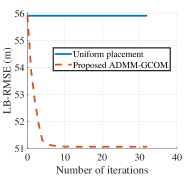
(a) βmax=120osubscript𝛽𝑚𝑎𝑥superscript120𝑜\beta_{max}=120^{o}.k¯MM=3subscript¯𝑘𝑀𝑀3\bar{k}_{MM}=3.
Refer to caption
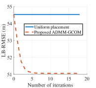
(b) βmax=200osubscript𝛽𝑚𝑎𝑥superscript200𝑜\beta_{max}=200^{o}.k¯MM=4subscript¯𝑘𝑀𝑀4\bar{k}_{MM}=4.
Refer to caption
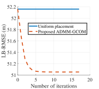
(c) βmax=280osubscript𝛽𝑚𝑎𝑥superscript280𝑜\beta_{max}=280^{o}.k¯MM=4subscript¯𝑘𝑀𝑀4\bar{k}_{MM}=4.
Refer to caption
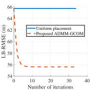
(d) βmax=360osubscript𝛽𝑚𝑎𝑥superscript360𝑜\beta_{max}=360^{o}.k¯MM=4subscript¯𝑘𝑀𝑀4\bar{k}_{MM}=4.
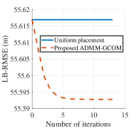
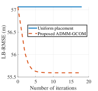
Figure 2: Convergence plots with different constrained angles in case A.
Refer to caption
(a) βmax=120osubscript𝛽𝑚𝑎𝑥superscript120𝑜\beta_{max}=120^{o}.k¯MM=2subscript¯𝑘𝑀𝑀2\bar{k}_{MM}=2.
Refer to caption
(b) βmax=200osubscript𝛽𝑚𝑎𝑥superscript200𝑜\beta_{max}=200^{o}.k¯MM=2subscript¯𝑘𝑀𝑀2\bar{k}_{MM}=2.
Refer to caption
(c) βmax=280osubscript𝛽𝑚𝑎𝑥superscript280𝑜\beta_{max}=280^{o}.k¯MM=2subscript¯𝑘𝑀𝑀2\bar{k}_{MM}=2.
Refer to caption
(d) βmax=360osubscript𝛽𝑚𝑎𝑥superscript360𝑜\beta_{max}=360^{o}.k¯MM=2subscript¯𝑘𝑀𝑀2\bar{k}_{MM}=2.
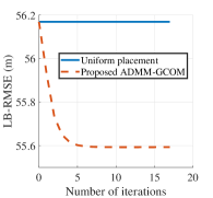
Figure 3: Convergence plots with different constrained angles in case B.

This section presents simulation results to evaluate the performance of the proposed ADMM-CGCOM, compared to the commonly used uniform placement strategy [18, 22].

Without loss of generality, the default settings are shown as follows: N=8𝑁8N=8, γ=2𝛾2\gamma=2, ri=1000msubscript𝑟𝑖1000mr_{i}=1000~{}\mathrm{m}, hi=100m,isubscript𝑖100mfor-all𝑖h_{i}=100~{}\mathrm{m},~{}\forall i. To make the simulation comprehensive, two typical cases named case A and case B are considered. In case A, the measurement conditions of UAVs are different. Specifically, half of the measuring noise variances are equal to 8dBm8dBm8~{}\mathrm{dBm} while the others are equal to 2dBm2dBm2~{}\mathrm{dBm}, i.e., σi2=8,i=1,,N2formulae-sequencesuperscriptsubscript𝜎𝑖28𝑖1𝑁2\sigma_{i}^{2}=8,~{}i=1,\cdots,\frac{N}{2} and σi2=2,i=N2+1,,Nformulae-sequencesuperscriptsubscript𝜎𝑖22𝑖𝑁21𝑁\sigma_{i}^{2}=2,~{}i=\frac{N}{2}+1,\cdots,N. In case B, the measurement conditions of UAVs are identical. Specifically, all measuring noise variance are equal to 4dBm4dBm4~{}\mathrm{dBm} , i.e.,σi2=4,i=1,,Nformulae-sequencesuperscriptsubscript𝜎𝑖24𝑖1𝑁\sigma_{i}^{2}=4,~{}i=1,\cdots,N. In addition, each UAV samples 101010 times quickly at the same measuring position and then averages the sampled RSSs to get the final measurement value.

Under the above settings, the proposed ADMM-CGCOM is used to optimize the geometric configuration of measuring UAVs, namely {βi}i=1Nsuperscriptsubscriptsubscript𝛽𝑖𝑖1𝑁\{\beta_{i}\}_{i=1}^{N}. To evaluate the optimized geometric configuration, a widely used lower bound of RMSE (abbreviated as LB-RMSE) is used as the performance metric of geometric configuration333LB-RMSE can be viewed as the lowest average distance error for any unbiased estimation. It is more intuitive and straightforward to evaluate geometric configurations than the determinant of FIM.. Mathematically, LB-RMSE =𝐅1(2,2)+𝐅1(3,3)absentsuperscript𝐅122superscript𝐅133=\sqrt{\mathbf{F}^{-1}(2,2)+\mathbf{F}^{-1}(3,3)}. Moreover, the convergence threshold of ADMM is 104superscript10410^{-4} and the convergence threshold of MM is 103superscript10310^{-3} in the simulation.

Refer to caption
(a) βmax=120osubscript𝛽𝑚𝑎𝑥superscript120𝑜\beta_{max}=120^{o}.
Refer to caption
(b) βmax=200osubscript𝛽𝑚𝑎𝑥superscript200𝑜\beta_{max}=200^{o}.
Refer to caption
(c) βmax=280osubscript𝛽𝑚𝑎𝑥superscript280𝑜\beta_{max}=280^{o}.
Refer to caption
(d) βmax=360osubscript𝛽𝑚𝑎𝑥superscript360𝑜\beta_{max}=360^{o}.
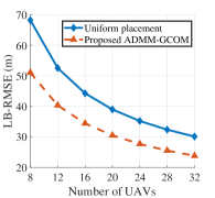
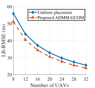
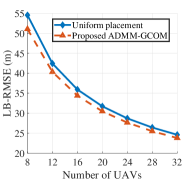
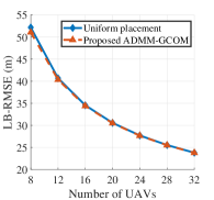
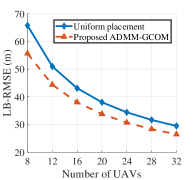
Figure 4: LB-RMSE versus the number of UAVs with different constrained angles in case A.
Refer to caption
(a) βmax=120osubscript𝛽𝑚𝑎𝑥superscript120𝑜\beta_{max}=120^{o}.
Refer to caption
(b) βmax=200osubscript𝛽𝑚𝑎𝑥superscript200𝑜\beta_{max}=200^{o}.
Refer to caption
(c) βmax=280osubscript𝛽𝑚𝑎𝑥superscript280𝑜\beta_{max}=280^{o}.
Refer to caption
(d) βmax=360osubscript𝛽𝑚𝑎𝑥superscript360𝑜\beta_{max}=360^{o}.
Figure 5: LB-RMSE versus the number of UAVs with different constrained angles in case B.

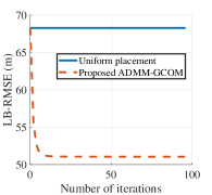
Fig. 2 shows the convergence curve of the proposed ADMM-CGCOM under different constrained angles in case A. As seen, starting from the uniform placement strategy, the proposed algorithm can further reduce LB-RMSE, thereby improving the performance of localization system. In addition, the improvement becomes obvious just after a few iterations. For example, after 101010 iterations, the proposed algorithm reduces LB-RMSE by nearly 6%percent66\% when βmax=280osubscript𝛽𝑚𝑎𝑥superscript280𝑜\beta_{max}=280^{o} and reduces LB-RMSE by nearly 25%percent2525\% when βmax=120osubscript𝛽𝑚𝑎𝑥superscript120𝑜\beta_{max}=120^{o}. Fig. 2 also shows that under different constrained angles, the proposed algorithm converges within 100100100 iterations while the average iteration time of the internal MM is no more than 444.

Fig. 3 shows the convergence curve of the proposed ADMM-CGCOM under different constrained angles in case B. Similar to case A as shown in Fig. 2, from Fig. 3, it is concluded that the proposed algorithm improves the performance of the localization system compared to the uniform placement strategy obviously just after a few iterations. Moreover, it is found that the improvement ratio of the proposed algorithm in case A (inconsistent measure conditions) is more significant than case B (identical measure conditions).

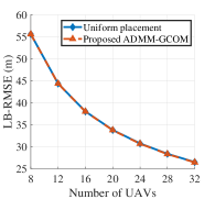
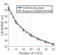
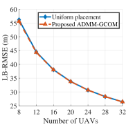
Fig. 4 presents the performance of the proposed ADMM-CGCOM versus the number of UAVs under different constrained angles in case A while Fig. 5 presents that in case B. From Fig. 4 and Fig. 5, it is observed that LB-RMSE decreases largely with increasing number of UAVs under different constrained angles. Moreover, it is seen that the proposed algorithm is over the uniform placement strategy with different scales of drone swarm, and the improvement ratio of the proposed algorithm with respect to the uniform placement strategy basically does not change versus the number of UAVs under different constrained angles.

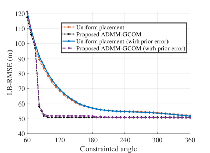
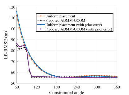
Theoretically, when using the proposed ADMM-CGCOM, the real position of source should be known. It is unrealistic. But with just small adjustment, the proposed algorithm can be used to refine a rough prior estimator in the practical scenario. Specifically, the prior estimator is used to replace the real position of source when using ADMM-CGCOM. In this way, the measuring positions of UAVs are obtained by ADMM-CGCOM, then UAVs can make effective measurement and estimation. Simulations about this practical scenario are shown in Fig. 6 and Fig. 7.

Fig. 6 presents the performance of the proposed ADMM-CGCOM versus the constrained angle considering both theoretical and practical scenarios in case A while Fig. 7 presents that in case B. In the practical scenario, the prior estimator is unbiased and the estimation error follows gaussian distribution with standard deviation equal to 12500m12500m\sqrt{12500}~{}\mathrm{m}. As observed from Fig. 6 and Fig. 7, the proposed algorithm is over the uniform placement strategy. Moreover, when the constrained angle exceeds a threshold (βmax>=97.5osubscript𝛽𝑚𝑎𝑥superscript97.5𝑜\beta_{max}>=97.5^{o} in case A and βmax>=105osubscript𝛽𝑚𝑎𝑥superscript105𝑜\beta_{max}>=105^{o} in case B), the performance of the proposed algorithm is basically unchanged as the constrained angle increases. Therefore, the proposed algorithm does not require a large constrained angle to achieve a considerable performance. Finally, as seen in Fig. 6 and Fig. 7, in the practical scenario, although the standard deviation of prior estimation is large, the performance of the proposed algorithm almost does not deviate from the theoretical value. Therefore the prior estimation can be refined well by the proposed algorithm.
Refer to caption
Figure 6:  LB-RMSE versus the constrained angle in case A.
Refer to caption
Figure 7:  LB-RMSE versus the constrained angle in case B.

VI Conclusion

In this paper we have investigated the geometric configuration of RSSD-based passive source localization system by drone swarm with spread angle constraint. We have formulated the constrained geometric configuration optimization problem under the D-optimization criterion, and transformed it from a multi-scalar form to a single-matrix matrix form, then proposed a numerical optimization method named ADMM-CGCOM. The proposed ADMM-CGCOM has been compared with the uniform placement strategy in simulations, where we have shown that ADMM-CGCOM leads to a lower LB-RMSE of the final estimation. Moreover, the function of ADMM-CGCOM on refining the initial estimation in the practical scenario has been demonstrated. Using the proposed ADMM-CGCOM, the effective measuring positions of drone swarm with constrained spread angle can be obtained.

Appendix A Proof of Theorem 1

Let λ¯¯𝜆\overline{\lambda} denote the mean of eigenvalues of 𝐓𝐓\mathbf{T}. From Eq. (III), it shows that 𝐓2×2𝐓superscript22\mathbf{T}\in\mathbb{R}^{2\times 2} and 𝐓𝐓\mathbf{T} is a symmetric matrix. Therefore,

|𝐓|𝐓\displaystyle\left|\mathbf{T}\right| =𝐓2+2λ¯2absentsuperscriptnorm𝐓22superscript¯𝜆2\displaystyle=-\left\|\mathbf{T}\right\|^{2}+2\overline{\lambda}^{2}
=𝐓2+12(i=1Nwiri2di4i=1Nwiridi2𝐠i2)2.absentsuperscriptnorm𝐓212superscriptsuperscriptsubscript𝑖1𝑁subscript𝑤𝑖superscriptsubscript𝑟𝑖2superscriptsubscript𝑑𝑖4superscriptnormsuperscriptsubscript𝑖1𝑁subscript𝑤𝑖subscript𝑟𝑖superscriptsubscript𝑑𝑖2subscript𝐠𝑖22\displaystyle=-\left\|\mathbf{T}\right\|^{2}+\frac{1}{2}\left(\sum_{i=1}^{N}w_{i}\frac{r_{i}^{2}}{d_{i}^{4}}-\left\|\sum_{i=1}^{N}w_{i}\frac{r_{i}}{d_{i}^{2}}\mathbf{g}_{i}\right\|^{2}\right)^{2}. (46)

Let 𝐔2×2𝐔superscript22\mathbf{U}\in\mathbb{R}^{2\times 2} represent an orthogonal matrix. For an arbitrary geometric configuration denoted as {𝐠i}i=1Nsuperscriptsubscriptsubscript𝐠𝑖𝑖1𝑁\{\mathbf{g}_{i}\}_{i=1}^{N}, we make an orthogonal transformation by 𝐔𝐔\mathbf{U} to obtain a new geometric configuration, denoted as {𝐠i}i=1Nsuperscriptsubscriptsubscriptsuperscript𝐠𝑖𝑖1𝑁\{\mathbf{g^{{}^{\prime}}}_{i}\}_{i=1}^{N}, i.e., 𝐠i=𝐔𝐠i,isubscriptsuperscript𝐠𝑖subscript𝐔𝐠𝑖for-all𝑖\mathbf{g^{{}^{\prime}}}_{i}=\mathbf{U}\mathbf{g}_{i},~{}\forall i. According to Eq. (III), it shows that 𝐓({𝐠i}i=1N)=𝐔𝐓({𝐠i}i=1N)𝐔T𝐓superscriptsubscriptsubscriptsuperscript𝐠𝑖𝑖1𝑁𝐔𝐓superscriptsubscriptsubscript𝐠𝑖𝑖1𝑁superscript𝐔𝑇\mathbf{T}\left(\{\mathbf{g^{{}^{\prime}}}_{i}\}_{i=1}^{N}\right)=\mathbf{U}\mathbf{T}\left(\{\mathbf{g}_{i}\}_{i=1}^{N}\right)\mathbf{U}^{T}. Then, we have

𝐓({𝐠i}i=1N)22subscriptsuperscriptnorm𝐓superscriptsubscriptsubscriptsuperscript𝐠𝑖𝑖1𝑁22\displaystyle\|\mathbf{T}\left(\{\mathbf{g^{{}^{\prime}}}_{i}\}_{i=1}^{N}\right)\|^{2}_{2}
=Tr(𝐔𝐓({𝐠i}i=1N)𝐔T𝐔𝐓({𝐠i}i=1N)T𝐔T)absentTr𝐔𝐓superscriptsubscriptsubscript𝐠𝑖𝑖1𝑁superscript𝐔𝑇𝐔𝐓superscriptsuperscriptsubscriptsubscript𝐠𝑖𝑖1𝑁𝑇superscript𝐔𝑇\displaystyle=\mathrm{Tr}\left(\mathbf{U}\mathbf{T}\left(\{\mathbf{g}_{i}\}_{i=1}^{N}\right)\mathbf{U}^{T}\mathbf{U}\mathbf{T}\left(\{\mathbf{g}_{i}\}_{i=1}^{N}\right)^{T}\mathbf{U}^{T}\right)
=𝐓({𝐠i}i=1N)2.absentsuperscriptnorm𝐓superscriptsubscriptsubscript𝐠𝑖𝑖1𝑁2\displaystyle=\|\mathbf{T}\left(\{\mathbf{g}_{i}\}_{i=1}^{N}\right)\|^{2}. (47)

Similarly,

i=1Nwiridi2𝐠i2=i=1Nwiridi2𝐠i2.superscriptnormsuperscriptsubscript𝑖1𝑁subscript𝑤𝑖subscript𝑟𝑖superscriptsubscript𝑑𝑖2superscriptsubscript𝐠𝑖2superscriptnormsuperscriptsubscript𝑖1𝑁subscript𝑤𝑖subscript𝑟𝑖superscriptsubscript𝑑𝑖2subscript𝐠𝑖2\displaystyle\left\|\sum_{i=1}^{N}w_{i}\frac{r_{i}}{d_{i}^{2}}\mathbf{g}_{i}^{{}^{\prime}}\right\|^{2}=\left\|\sum_{i=1}^{N}w_{i}\frac{r_{i}}{d_{i}^{2}}\mathbf{g}_{i}\right\|^{2}. (48)

According to Eq. (A), Eq. (A) and Eq. (48), we have |𝐓|=|𝐓|superscript𝐓𝐓|\mathbf{T}^{{}^{\prime}}|=|\mathbf{T}|. Therefore, the effectiveness of geometric configuration (the determinant of FIM) is unchanged after the orthogonal transformation. Moreover, referring [18], orthogonal transformation means horizontal overall rotation or horizontal overall with respect to the source in the focused localization system.

Appendix B The Global Optimal Property of 𝐆Tksubscriptsuperscript𝐆𝑘𝑇\mathbf{G}^{k}_{T}

According to the definition of 𝐌𝐌\mathbf{M}, Lρksuperscriptsubscript𝐿𝜌𝑘L_{\rho}^{k} in Eq. (IV-C) can be expressed as

Lρksuperscriptsubscript𝐿𝜌𝑘\displaystyle L_{\rho}^{k} =ρ2Tr(𝐆T𝐌𝐆)+Tr(𝐐kT𝐆)+αkabsent𝜌2Trsuperscript𝐆𝑇𝐌𝐆Trsuperscript𝐐𝑘𝑇𝐆superscript𝛼𝑘\displaystyle=\frac{\rho}{2}\mathrm{Tr}\left(\mathbf{G}^{T}\mathbf{M}\mathbf{G}\right)+\mathrm{Tr}\left(\mathbf{Q}^{kT}\mathbf{G}\right)+\alpha^{k}
=ρ2i=1N𝐠iT𝐌𝐠i+i=1N𝐪ikT𝐠i,absent𝜌2superscriptsubscript𝑖1𝑁superscriptsubscript𝐠𝑖𝑇subscript𝐌𝐠𝑖superscriptsubscript𝑖1𝑁superscriptsubscript𝐪𝑖𝑘𝑇subscript𝐠𝑖\displaystyle=\frac{\rho}{2}\sum_{i=1}^{N}\mathbf{g}_{i}^{T}\mathbf{M}\mathbf{g}_{i}+\sum_{i=1}^{N}\mathbf{q}_{i}^{kT}\mathbf{g}_{i}, (49)

where 𝐐kT=𝐂kT𝐁12𝐃superscript𝐐𝑘𝑇superscript𝐂𝑘𝑇superscript𝐁12𝐃\mathbf{Q}^{kT}=\mathbf{C}^{kT}\mathbf{B}^{\frac{1}{2}}\mathbf{D} and 𝐪ikTsuperscriptsubscript𝐪𝑖𝑘𝑇\mathbf{q}_{i}^{kT} is the i𝑖i-th row of 𝐐kTsuperscript𝐐𝑘𝑇\mathbf{Q}^{kT}. The second-order derivative of Lρksuperscriptsubscript𝐿𝜌𝑘L_{\rho}^{k} with respect to 𝐠isubscript𝐠𝑖\mathbf{g}_{i} is given by

𝐠i2Lρ(𝐗k+1,𝐆,𝐕k)=ρ𝐌𝟎,i.formulae-sequencesuperscriptsubscriptsubscript𝐠𝑖2subscript𝐿𝜌superscript𝐗𝑘1𝐆superscript𝐕𝑘𝜌𝐌succeeds-or-equals0for-all𝑖\displaystyle\nabla_{\mathbf{g}_{i}}^{2}L_{\rho}(\mathbf{X}^{k+1},\mathbf{G},\mathbf{V}^{k})=\rho\mathbf{M}\succeq\mathbf{0},~{}\forall i. (50)

Therefore, the objective function of subproblem (25b)) is a convex function with respect to 𝐠isubscript𝐠𝑖\mathbf{g}_{i}, ifor-all𝑖\forall i. But the constraint 𝒟𝒟\mathcal{D} in subproblem (25b) is not convex. Therefore, the convergence of MM may be local optimal. However, the global optimal property of it is demonstrated by the following analysis.

First, we slack 𝒟𝒟\mathcal{D} to generate a new set denoted as 𝒟¯¯𝒟\overline{\mathcal{D}} as follows.

𝒟¯={𝐆|𝐠iT𝐠i1,𝐠i𝐠0,i}.¯𝒟conditional-set𝐆formulae-sequencesuperscriptsubscript𝐠𝑖𝑇subscript𝐠𝑖1subscript𝐠𝑖subscript𝐠0for-all𝑖\displaystyle\overline{\mathcal{D}}=\{\mathbf{G}|\mathbf{g}_{i}^{T}\mathbf{g}_{i}\leq 1,~{}\mathbf{g}_{i}\geq\mathbf{g}_{0},~{}\forall i\}. (51)

Assume 𝐆e𝒟¯subscript𝐆𝑒¯𝒟\mathbf{G}_{e}\in\overline{\mathcal{D}},𝐆f𝒟¯subscript𝐆𝑓¯𝒟\mathbf{G}_{f}\in\overline{\mathcal{D}}. Let 𝐠e,isubscript𝐠𝑒𝑖\mathbf{g}_{e,i} denote the transpose of the i𝑖i-th row of 𝐆esubscript𝐆𝑒\mathbf{G}_{e} and 𝐠f,isubscript𝐠𝑓𝑖\mathbf{g}_{f,i} denote the transpose of the i𝑖i-th row of 𝐆fsubscript𝐆𝑓\mathbf{G}_{f}. For any (α,β)𝛼𝛽(\alpha,\beta) satisfying 0α10β1α+β=10𝛼10𝛽1𝛼𝛽10\leq\alpha\leq 1\cup 0\leq\beta\leq 1\cup\alpha+\beta=1, we have

α𝐠e,i+β𝐠f,i[(α+β)𝐠0(1)(α+β)𝐠0(2)]𝐠0,𝛼subscript𝐠𝑒𝑖𝛽subscript𝐠𝑓𝑖matrix𝛼𝛽subscript𝐠01𝛼𝛽subscript𝐠02subscript𝐠0\displaystyle\alpha\mathbf{g}_{e,i}+\beta\mathbf{g}_{f,i}\geq\begin{bmatrix}(\alpha+\beta)\mathbf{g}_{0}(1)&(\alpha+\beta)\mathbf{g}_{0}(2)\end{bmatrix}\geq\mathbf{g}_{0}, (52)
(α𝐠e,i+β𝐠f,i)T(α𝐠e,i+β𝐠f.i)superscript𝛼subscript𝐠𝑒𝑖𝛽subscript𝐠𝑓𝑖𝑇𝛼subscript𝐠𝑒𝑖𝛽subscript𝐠formulae-sequence𝑓𝑖\displaystyle(\alpha\mathbf{g}_{e,i}+\beta\mathbf{g}_{f,i})^{T}(\alpha\mathbf{g}_{e,i}+\beta\mathbf{g}_{f.i})
=α2𝐠e,i2+β2𝐠f,i2+2αβ𝐠e,iT𝐠f,i(α+β)2=1.absentsuperscript𝛼2superscriptnormsubscript𝐠𝑒𝑖2superscript𝛽2superscriptnormsubscript𝐠𝑓𝑖22𝛼𝛽superscriptsubscript𝐠𝑒𝑖𝑇subscript𝐠𝑓𝑖superscript𝛼𝛽21\displaystyle=\alpha^{2}\|\mathbf{g}_{e,i}\|^{2}+\beta^{2}\|\mathbf{g}_{f,i}\|^{2}+2\alpha\beta\mathbf{g}_{e,i}^{T}\mathbf{g}_{f,i}\leq(\alpha+\beta)^{2}=1. (53)

Therefore, 𝒟¯¯𝒟\overline{\mathcal{D}} is a convex set.

Then, taking 𝒟¯¯𝒟\overline{\mathcal{D}} as the constraint, a new subproblem based on subproblem (25b) is considered as follows.

𝐆k+1=argmin𝐆𝒟¯Lρ(𝐗k+1,𝐆,𝐕k).superscript𝐆𝑘1subscriptargmin𝐆¯𝒟subscript𝐿𝜌superscript𝐗𝑘1𝐆superscript𝐕𝑘\displaystyle\mathbf{G}^{k+1}=\mathop{\mathrm{argmin}}_{\mathbf{G}\in\overline{\mathcal{D}}}L_{\rho}(\mathbf{X}^{k+1},\mathbf{G},\mathbf{V}^{k}). (54)

From above, it shows that subproblem (54) is convex.

Finally, compare the two subproblems. When using the MM algorithm in Section IV-C, it is easy to verify that the obtained solution of subproblem (54) (𝐆Tksubscriptsuperscript𝐆𝑘𝑇\mathbf{G}^{k}_{T}) is the same as that in subproblem (25b). Note that 𝐆Tksubscriptsuperscript𝐆𝑘𝑇\mathbf{G}^{k}_{T} must be a local optimal solution of subproblem (54). And it is well known that the local optimal solution of a convex problem is also the global optimal solution. Therefore, 𝐆Tksubscriptsuperscript𝐆𝑘𝑇\mathbf{G}^{k}_{T} is global optimal on subproblem (54). Since 𝒟𝒟¯𝒟¯𝒟\mathcal{D}\in\overline{\mathcal{D}}, subproblem (54) is a slack version of subproblem (25b), it can be concluded that 𝐆Tksubscriptsuperscript𝐆𝑘𝑇\mathbf{G}^{k}_{T} is also the global optimal solution of subproblem (25b).

References

  • [1] K. Ho and M. Sun, “Passive source localization using time differences of arrival and gain ratios of arrival,” IEEE Transactions on Signal Processing, vol. 56, no. 2, pp. 464–477, 2008.
  • [2] K. Dogancay, “UAV path planning for passive emitter localization,” IEEE Transactions on Aerospace and Electronic systems, vol. 48, no. 2, pp. 1150–1166, 2012.
  • [3] M. Z. Win, Y. Shen, and W. Dai, “A theoretical foundation of network localization and navigation,” Proceedings of the IEEE, vol. 106, no. 7, pp. 1136–1165, 2018.
  • [4] D.-H. Kim, K. Lee, M.-Y. Park, and J. Lim, “UAV-based localization scheme for battlefield environments,” in MILCOM 2013-2013 IEEE Military Communications Conference.   IEEE, 2013, pp. 562–567.
  • [5] X. Jiang, N. Li, Y. Guo, D. Yu, and S. Yang, “Localization of multiple RF sources based on bayesian compressive sensing using a limited number of UAVs with airborne RSS sensor,” IEEE Sensors Journal, vol. 21, no. 5, pp. 7067–7079, 2020.
  • [6] W. Wang, P. Bai, X. Liang, J. Zhang, and L. He, “Performance analysis and path planning for UAVs swarms based on RSS measurements,” Aerospace Science and Technology, vol. 81, pp. 157–166, 2018.
  • [7] X. Cheng, W. Shi, W. Cai, W. Zhu, T. Shen, F. Shu, and J. Wang, “Communication-efficient coordinated RSS-based distributed passive localization via drone cluster,” IEEE Transactions on Vehicular Technology, vol. 71, no. 1, pp. 1072–1076, 2021.
  • [8] F. Shu, Y. Qin, T. Liu, L. Gui, Y. Zhang, J. Li, and Z. Han, “Low-complexity and high-resolution DOA estimation for hybrid analog and digital massive MIMO receive array,” IEEE Transactions on Communications, vol. 66, no. 6, pp. 2487–2501, 2018.
  • [9] E. Xu, Z. Ding, and S. Dasgupta, “Source localization in wireless sensor networks from signal time-of-arrival measurements,” IEEE Transactions on Signal Processing, vol. 59, no. 6, pp. 2887–2897, 2011.
  • [10] K. Ho and Y. Chan, “Solution and performance analysis of geolocation by TDOA,” IEEE Transactions on Aerospace and Electronic Systems, vol. 29, no. 4, pp. 1311–1322, 1993.
  • [11] A. J. Weiss, “On the accuracy of a cellular location system based on RSS measurements,” IEEE transactions on vehicular technology, vol. 52, no. 6, pp. 1508–1518, 2003.
  • [12] H. Lohrasbipeydeh, T. A. Gulliver, and H. Amindavar, “Unknown transmit power RSSD based source localization with sensor position uncertainty,” IEEE Transactions on Communications, vol. 63, no. 5, pp. 1784–1797, 2015.
  • [13] N. Patwari, J. N. Ash, S. Kyperountas, A. O. Hero, R. L. Moses, and N. S. Correal, “Locating the nodes: cooperative localization in wireless sensor networks,” IEEE Signal processing magazine, vol. 22, no. 4, pp. 54–69, 2005.
  • [14] H. Lohrasbipeydeh, T. A. Gulliver, and H. Amindavar, “A minimax SDP method for energy based source localization with unknown transmit power,” IEEE Wireless Communications Letters, vol. 3, no. 4, pp. 433–436, 2014.
  • [15] S. M. Kay, Fundamentals of statistical signal processing: estimation theory.   Prentice-Hall, Inc., 1993.
  • [16] D. Ucinski, Optimal measurement methods for distributed parameter system identification.   CRC press, 2004.
  • [17] X. Cheng, F. Shu, Y. Li, Z. Zhuang, D. Wu, and J. Wang, “Optimal measurement of drone swarm in RSS-based passive localization with region constraints,” IEEE Open Journal of Vehicular Technology, vol. 4, pp. 1–11, 2022.
  • [18] S. Zhao, B. M. Chen, and T. H. Lee, “Optimal sensor placement for target localisation and tracking in 2D and 3D,” International Journal of Control, vol. 86, no. 10, pp. 1687–1704, 2013.
  • [19] S. Xu, Y. Ou, and W. Zheng, “Optimal sensor-target geometries for 3-D static target localization using received-signal-strength measurements,” IEEE Signal Processing Letters, vol. 26, no. 7, pp. 966–970, 2019.
  • [20] N. Sahu, L. Wu, P. Babu, B. S. MR, and B. Ottersten, “Optimal sensor placement for source localization: A unified ADMM approach,” IEEE Transactions on Vehicular Technology, vol. 71, no. 4, pp. 4359–4372, 2022.
  • [21] J. Li, K. Doğançay, and H. Hmam, “Optimal angular sensor separation for DRSS localization,” in 2022 IEEE 12th Sensor Array and Multichannel Signal Processing Workshop (SAM).   IEEE, 2022, pp. 326–330.
  • [22] A. Heydari, M. Aghabozorgi, and M. Biguesh, “Optimal sensor placement for source localization based on RSSD,” Wireless Networks, vol. 26, pp. 5151–5162, 2020.
  • [23] A. Heydari and M.-R. Aghabozorgi, “Sensor placement for RSSD-based localization: Optimal angular placement and sequential sensor placement,” Physical Communication, vol. 42, p. 101134, 2020.
  • [24] M. Sadeghi, F. Behnia, and R. Amiri, “Optimal sensor placement for 2-D range-only target localization in constrained sensor geometry,” IEEE Transactions on Signal Processing, vol. 68, pp. 2316–2327, 2020.
  • [25] ——, “Optimal geometry analysis for TDOA-based localization under communication constraints,” IEEE Transactions on Aerospace and Electronic Systems, vol. 57, no. 5, pp. 3096–3106, 2021.
  • [26] Y. Liang and Y. Jia, “Constrained optimal placements of heterogeneous range/bearing/RSS sensor networks for source localization with distance-dependent noise,” IEEE Geoscience and Remote Sensing Letters, vol. 13, no. 11, pp. 1611–1615, 2016.
  • [27] S. P. Boyd and L. Vandenberghe, Convex optimization.   Cambridge university press, 2004.
  • [28] S. Boyd, N. Parikh, E. Chu, B. Peleato, J. Eckstein et al., “Distributed optimization and statistical learning via the alternating direction method of multipliers,” Foundations and Trends® in Machine learning, vol. 3, no. 1, pp. 1–122, 2011.
  • [29] Y. Xingdong, S. Runqing, X. Weiwei, L. Shihui, and D. Sanqin, “A note on Von Neumann’s trace inequality,” Journal of Nanjing Normal University(Natural Science Edition), 2018.
  • [30] R. A. Horn and C. R. Johnson, Matrix analysis.   Cambridge university press, 2012.
  • [31] Y. Sun, P. Babu, and D. P. Palomar, “Majorization-minimization algorithms in signal processing, communications, and machine learning,” IEEE Transactions on Signal Processing, vol. 65, no. 3, pp. 794–816, 2016.
  • [32] M. Hong, Z.-Q. Luo, and M. Razaviyayn, “Convergence analysis of alternating direction method of multipliers for a family of nonconvex problems,” SIAM Journal on Optimization, vol. 26, no. 1, pp. 337–364, 2016.
  • [33] Y. Wang, W. Yin, and J. Zeng, “Global convergence of ADMM in nonconvex nonsmooth optimization,” Journal of Scientific Computing, vol. 78, pp. 29–63, 2019.
  • [34] Q. Liu, X. Shen, and Y. Gu, “Linearized ADMM for nonconvex nonsmooth optimization with convergence analysis,” IEEE access, vol. 7, pp. 76 131–76 144, 2019.
  • [35] S. Xu, M. Rice, and F. Rice, “Optimal TOA-sensor placement for two target localization simultaneously using shared sensors,” IEEE Communications Letters, vol. 25, no. 8, pp. 2584–2588, 2021.
  • [36] J. T. Isaacs, D. J. Klein, and J. P. Hespanha, “Optimal sensor placement for time difference of arrival localization,” in Proceedings of the 48h IEEE Conference on Decision and Control (CDC) held jointly with 2009 28th Chinese Control Conference.   IEEE, 2009, pp. 7878–7884.