Evidence for Spatial Separation of Galactic Dust Components

Abstract

We present an implementation of a Bayesian mixture model using Hamiltonian Monte Carlo (HMC) techniques to search for spatial separation of Galactic dust components. Utilizing intensity measurements from Planck High Frequency Instrument (HFI), we apply this model to high-latitude Galactic dust emission. Our analysis reveals a strong preference for a spatially-varying two-population dust model in intensity, with each population being well characterized by a single-component dust spectral-energy distribution (SED). While no spatial information is built into the likelihood, our investigation unveils spatially coherent structures with high significance, pointing to a physical origin for the observed spatial separation. These results are robust to our choice of likelihood and of input data. Furthermore, they are favored over a single-component dust model by Bayesian evidence calculations. Incorporating IRAS 100 $\mu m$ to constrain the Wein-side of the blackbody function, we find the dust populations differ at the $2.5\sigma$ level in the spectral index ($\beta_{d}$) vs. temperature $(T_{d})$ plane. The presence of multiple dust populations has implications for component separation techniques frequently employed in the recovery of the cosmic microwave background.

tablenum SIXtablenum

1 Introduction

Understanding Galactic dust emission in the millimeter (mm) wavelength range plays an important role in cosmic microwave background (CMB) science. This diffuse emission, originating from $\sim$20 K thermal emission of interstellar dust grains within our Milky Way galaxy, peaks at $\sim$2 THz, but remains significant relative to the polarized CMB anisotropy at frequencies above about 100 GHz. Understanding and characterizing Galactic dust emission is essential for accurately modeling its emission to correct for its distortions of the underlying CMB signal.

The properties of interstellar dust grains, including their size and shape, composition, distribution, and temperature, all influence the resulting radiation (draineli_2001, draine_2007, draine_2009). In the context of component separation, the complexity of interstellar dust is typically flattened; its spectral energy distribution (SED) is modeled as a modified blackbody, with emissions resembling that of a thermal blackbody at temperature $T_{d}$ and a fractional emissivity that scales with frequency according to its spectral index $\beta_{d}$. (brandt1994; Finkbeiner_1999).

Much of our understanding of the mm-wave emission of dust comes from two satellite data sets: first from IRAS (iras) and then Planck (planck_I_2018, planck_III_2018).

Planck uses three bands, 353, 545 and 857 GHz, in combination with DIRBE IRAS 100 $\mu m$ to construct an all-sky model of dust-emission parameterized by a single-component emissivity spectral index and temperature $(\beta_{d},T_{d})$ that vary along the line-of-sight (planck_XI_2013, planck_XVII_2014).

Meisner and Finkbeiner observed that there is a flattening of the SED model at lower frequencies (100-350 GHz) that departs from a single-component SED. Instead, they proposed a two-component model that incorporates the superposition of a hot and cold component to more accurately capture the shape of the dust SED at these lower frequencies (Finkbeiner_1999; Meisner_2014).

Furthermore, Hensley and Draine have shown that dust grains with distinct sizes and compositions will attain different temperatures, even in the same radiative environment. They have developed a physically motivated two-component dust model positing that dust emission originates from a mixture of carbonaceous and silicate sources (Hensley_2018, Hensley_2021). In their recent work, however, Hensley and Draine state that the observed lack of frequency dependence in the far-infrared polarization fraction is most naturally explained by a single-composition dust model (hensley2022astrodustpah).

Given the inherent complexity of Galactic dust emission, there exists considerable scope for refining modeling efforts. In this paper, we exclusively examine dust emission in intensity and present an approach that looks for SED variations in the spatial domain. We identify variations of the SED and assign them to different global populations of dust. These dust populations, we believe, have different optical properties that can arise due to differences in their physical characteristics or their respective radiative environment.

In section 2.1, we first describe a generic method for linear regression with uncertainties. Then, in section 2.2, we utilize this method to build a likelihood model for dust emission with multiple populations. In section 3, we demonstrate that this likelihood is unbiased and can recover components even in highly mixed situations. In section 4, we describe the preprocessing steps for this analysis, and section 5 provides the primary result of this analysis. In section 6, we look for the same features in the region observed by the Spider balloon experiment (filippini_spider, Rahlin2014, Gualtieri2018LTD), a relatively large ($\sim 5\%$) and clean patch of the sky used for CMB B-mode studies. Then, in section 7 explore several analysis choices and how these choices affect the results. In section 8, we calculate the Bayesian evidence to determine which model is most favored. Lastly, in section 9, we fit a modified blackbody model to the multiple populations.

2 Method

2.1 “Mahalanobis” regression in the generic case with X,Y uncertainties

Figure 1: Diagram of fitting a point ${\bf Z_{i}}$ with covariance ${\bf\Sigma_{i}}$ to a model line $(\theta,b)$. A vector ${\bf v}$ perpendicular to the slope $\theta$ is constructed so that we can project the point ${\bf Z_{i}}$ onto the line such that the perpendicular distance is given by $\Delta_{i}={\bf v}^{\mathrm{T}}{\bf Z_{i}}-b\cos\theta$. While this may be the minimum geometric distance, the minimum Mahalanobis distance is along the vector ${\bf u_{i}}$. Then the uncertainties $\Sigma_{i}$ are projected along the vector ${\bf u_{i}}$ to the line: $S_{i}={\bf u^{\mathrm{T}}_{i}\Sigma_{i}u_{i}}$.

Traditional linear regression assumes that independent variables (the abscissa) are known with certainty. In many real-world scenarios, however, uncertainties and errors in data collection can affect both the abscissa and ordinate. Indeed, in our analysis of the Planck data, the uncertainties are of a similar order to each other. Ignoring or underestimating these uncertainties when using standard methods, such as ordinary least squares, can lead to biased parameter estimates.

Handling ”Errors-in-variables” in linear regression is a challenging topic. Unlike the standard approach, incorporating uncertainties in both the abscissa and ordinate requires sophisticated methods to account for uncertainty propagation. Moreover, there is no consensus on the best approach (hogg_likelihood, tullyfisher_fitting).

Orthogonal regression is a popular approach that minimizes the orthogonal distance of all the points to a regression line. While the orthogonal distance is the smallest geometric distance, however, it may not correspond to the smallest distance in probability space in cases where errors in the abscissa and ordinate are unequal. We make a modification to the method to minimize the Mahalanobis distance between each point $i$ and the regression line $k$. Therefore, we find the distance along a unit-vector ${\bf u_{i}}$ whose direction is described by the angle $\phi$,

$$\phi=\arctan\left(-\frac{1}{\tan\theta}\frac{\sigma_{y}^{2}}{\sigma_{x}^{2}}\right)$$ (1)

and the uncertainties of each point $i$ is also projected along ${\bf u_{i}}$. The derivation of this expression can be found in Appendix LABEL:sec:appendix_derivation. We call this method “Mahalanobis regression”.

This regression method, similar to orthogonal regression, fails to capture the variance along the regression line. Handling the full uncertainty in the generic case is computationally challenging. Rather than reducing dimensionality by using a regression model that has two variables, namely a slope and an offset, a fully generic regression would require $N+2$ variables to account for $N$ data points. Each observed point represents a sample from a two-dimensional Gaussian distribution, originating from a pair of “true” values ($x^{*},y^{*}$) within a regression model.

However, this approach becomes computationally impractical when considering the construction of a mixture model in the following section. Therefore, we chose to reduce the dimensionality of the problem using Mahalanobis regression as described.

2.2 Gaussian Mixture Model

We introduce a generic Gaussian Mixture Model (GMM), in which a given map pixel $i$ can belong to one of $K$ populations. Depending on the specifics of the analysis, certain parameters can be constrained to have a fixed value of zero.

We parameterize each population by its slope $\theta_{k}$, calibration offset $b_{k}$, and assign each point $i$ a population using $q_{i,k}$. $q_{i,k}$ is a boolean value for point $i$ to belong in population $k$. We define $q_{i,k}=0$ as a rejection of point $i$ from population $k$, forcing that point to be assigned to a different population.

We fit this model to a scatter plot of points using Mahalanobis regression, as defined in the previous section, performed by maximizing the following likelihood:

$$\mathcal{L}(\{q_{i,k}\},\theta_{k}, b_{k},V_{k},p_{k})=$$

$$\begin{aligned} \prod_{i}\prod_{k}&\left[\frac{1}{\sqrt{2\pi(\Sigma_{i,k}+V_{k})}}\right.\\ &\times\left.\exp\left(-\frac{(\Delta_{i,k}/\cos(|\phi|+\theta-\pi/2))^{2}}{2(\Sigma_{i,k}+V_{k})}\right)\right]^{q_{i,k}}\end{aligned}$$ (2)

$$\Delta_{i,k} ={\bf v}\left(\theta_{k}\right)^{\mathrm{T}}Z_{i}-b_{k}\cos(\theta_{k})=-\sin\left(\theta_{k}\right)x_{i}+\cos\left(\theta_{k}\right)(y_{i}-b_{k})$$ (3)

$$\Sigma_{i,k} ={\bf u_{i}}\left(\theta_{k}\right)^{\mathrm{T}}\begin{pmatrix}\sigma_{x}^{2}&0\\ 0&\sigma_{y}^{2}\end{pmatrix}{\bf u_{i}}\left(\theta_{k}\right)$$ (4)

The orthogonal distance of point $i$ to line $k$ is represented by $\Delta_{i,k}$. Then, the Mahalanobis distance can be computed by simple trigonometry: $\Delta_{i,k}/\cos(|\phi|+\theta-\pi/2)$. To get the uncertainties, we use eq. 4 to project the covariance of each data point along the Mahalanobis distance, ${\bf v}$, resulting in the scalar value $\Sigma_{i,k}$. Furthermore, we assign an additional variance term $V_{k}$ to each population, representing the intrinsic scatter fitted for that population.

We further impose a prior on $q_{i}$ of the form of a Dirichlet-Multinomial distribution:

$$q_{i,k}\sim\text{DirMult}(n=1,\{p_{A},p_{B},\cdots p_{K}\})$$ (5)

The hyperparameters $\{p_{A}\cdots p_{K}\}$ have an additional constraint that $\sum_{k}p_{k}=1$ so that the prior distribution therefore has an expected value of $p_{k}$ for each population $k$. This has a physically motivated interpretation that $p_{k}$ represents the global fraction of points belonging to the $k^{\mathrm{th}}$ population.

In the common case where there are only two populations, this distribution reduces to the beta-binomial distribution. Drawing from this prior can be thought of as a two-step process: first sample from a Beta($\alpha=p_{A},\beta\ =1-p_{A}$) to get a probability $\pi_{i,A}$ for each point, then run a Bernoulli trial with probability $\{\pi_{i,A},(1-\pi_{i,A})\}$ to determine the assignment $q_{i}$ of this point. With multiple populations, this can be conceptually generalized to drawing a probability from a Dirichlet distribution and then drawing from a categorical distribution.

We treat $\{p_{A}\cdots p_{K}\}$ as global hyper-parameters, and fit for them simultaneously alongside the other parameters. This likelihood construction limits the propagation of noise into our final population assignments: statistically indistinct points will largely be determined by the prior with $\pi_{i,A}=p_{A}$. Effectively, these points are assigned to a population based on the prevalence of that population.

2.3 Implementation in Python

Scikit-learn is perhaps the most well-established and widely used open-source implementation of GMMs (scikit-learn). The code is based on the Expectation-Maximization (EM) algorithm (em_paper). While this algorithm is computationally efficient and converges far faster than Monte Carlo methods, EM methods provide only a point estimate of the MLE. Monte Carlo methods, on the other hand, naturally estimate uncertainty by sampling the posterior distribution and are therefore applied in this analysis.

Additionally, we need estimates of $\pi_{i,k}$, the probability a given pixel belongs to a population $k$. Therefore, we need to sample the full likelihood (eq. 2),   including the discrete variables, $q_{i,k}$, which is a task not handled by all probabilistic programming packages (stan). This analysis is computationally challenging, because $N$ is the number of pixels in our region of interest, of order $10^{5}$, and the probability volume is $\sim K^{N}$, representing an enormous space for MCMCs. The computational cost of any Monte-Carlo algorithm can be expressed as $\mathcal{O}(M*N)$ where $M$ is the number of Monte-Carlo samples and $N$ is the dimensionality. This is because proposing new states scales linearly with the number of dimensions. However, each proposal step is not independent; for a random-walker algorithm, $M\sim\mathcal{O}(N)$ generates an independent point (neal_hmc). Therefore, a Metropolis-Hastings algorithm is expected to scale as $\mathcal{O}(N^{2})$ making it computationally impossible to use rejection samplers in high-dimensional spaces.

Hamiltonian Monte-Carlo (HMC) instead uses dynamical properties to more efficiently generate independent points (hmc). The proposals are more effective for exploring high-dimensional spaces, making them particularly useful for complex Bayesian inference. Independent points scale according to $M\sim N^{\frac{1}{4}}$ (neal_hmc, beskos2010optimal), so the total algorithm scales as $\mathcal{O}(N^{\frac{5}{4}})$.

This analysis leverages NumPyro, which is a probabilistic programming language that relies on JAX for automatic differentiation of functions (phan2019composable, bingham2019pyro) and efficiently generates HMC samples.

3 Validations on Simulations

Figure 2: We conducted two validation analyses using Mahalanobis regression (eq 2) on the same input dataset. On the left, we assumed two distinct populations ($m_{0},m_{1}$) and estimated a global population fraction parameter $(p_{A})$ without including offset or additional variance parameters $(b_{k}=0,V_{k}=0)$. On the right, the hyperparameter $p_{A}$ is turned off and the prior probability of each point $\pi_{i}$ is instead drawn from a uniform distribution. These fits are labeled “Mix. fit” for the two populations respectively. These are compared to “Single fit,” which is the Mahalanobis regression for each of the input populations. The colors represent the probability of a data point $p_{i}$ belonging to population 1. On the left, even with two highly overlapping populations, we recover both the intrinsic relationship and can distinguish points to their respective population with high confidence. On the right, without this global hyperparameter, points with an equivalent likelihood of belonging to either population fit $\pi_{i}\sim 0.5$. Because the steeper blue population intrinsically has a far smaller prevalence, this equal assignment biases the slope downward, and we fail to recover the input slopes.

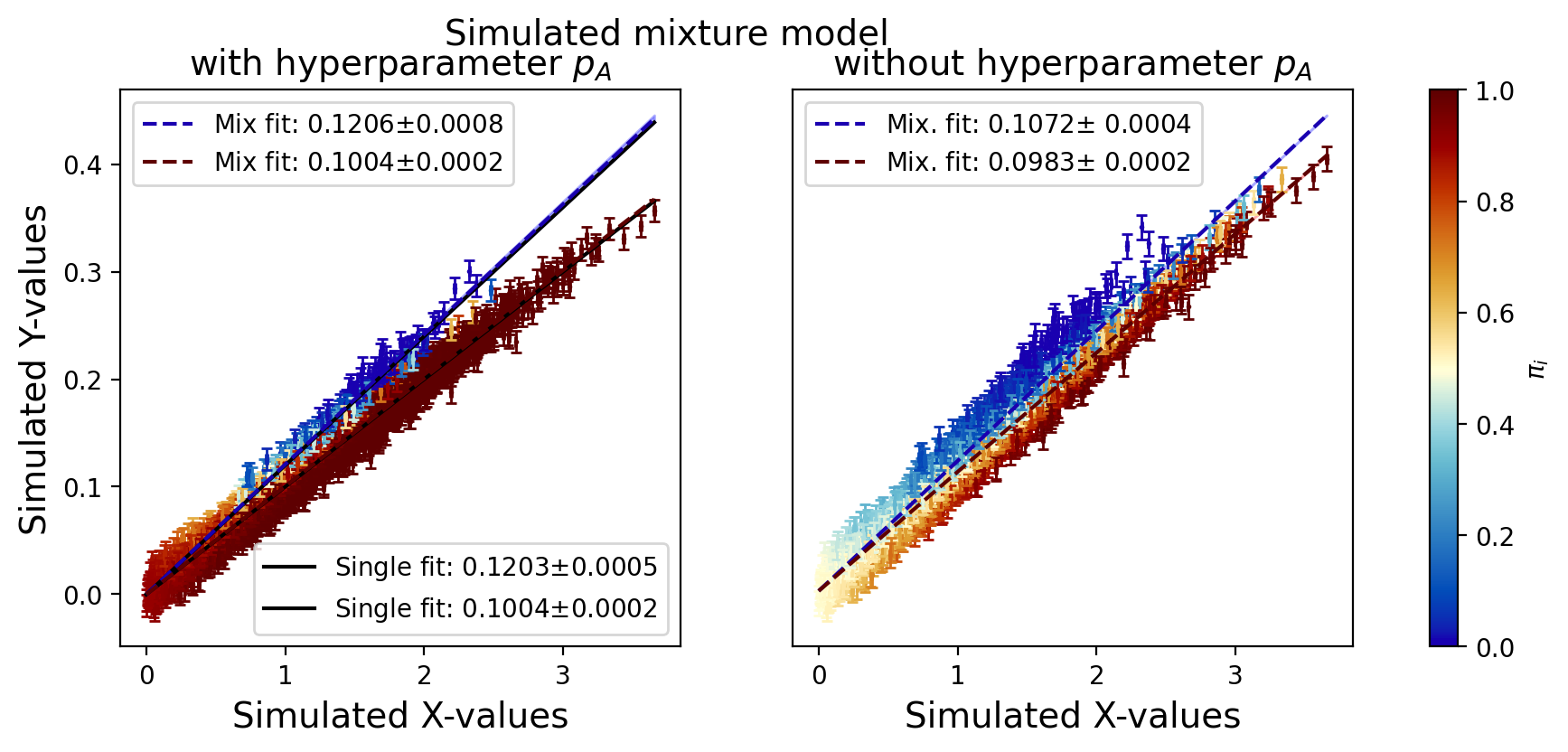
To validate this analysis method, we can generate data consisting of two populations with similar slopes and show that the pipeline is capable of distinguishing the populations. Figure 2 shows an example of such a test, where two populations with very different proportions $(N_{\{0,1\}}=\{200,2000\})$ and input slopes $(\theta_{\{0,1\}}=\{0.10,0.12\})$ are observed with highly overlapping populations. In this simulated analysis, we do not include an offset $b_{k}=0$ or variance $V_{k}=0$ in the model. The figures then differ on whether they include the fitted hyperparameter $p_{k}$ in the analysis.

On the left, we use the nominally described method, and we are able to accurately distinguish points that belong to each population in the extremes with high probability $\pi_{i}$. Points clustered in the middle, well within the uncertainties for either model $\theta_{\{0,1\}}$, are preferentially assigned to the population that is more numerous. The fitted hyperparameter $p_{A}$ can be interpreted as the global population fraction. In the case where a point’s uncertainty makes it indistinguishable from both populations, $p_{A}$ acts as a prior on how to assign that point through the $\pi_{i}$’s.

On the right, we disable the hyperparameter, $p_{k}$, and instead draw $\pi_{i}$ from a uniform prior ranging from 0 to 1. In this case, points clustered between the populations are assigned $\pi_{i}\approx 0.5$ indicating no preference for either population. However, due to the difference in prevalence of the two populations, there is an over-assignment of points to the blue population, introducing a bias in the recovered slope.

While a uniform prior may seem impartial at the individual data point level, its effects are less innocent on a global scale. A uniform distribution is equivalent to a Beta distribution with fixed $\alpha=\beta=1$, resulting in a mean of 0.5. The presence of this uniform prior is globally informative, leading to incorrect assignments of populations and ultimately causing a failure in the recovery of the simulated inputs.

For this reason, we include the fitted hyperparameter $p_{k}$ in all configurations when running the data analysis.

4 Preprocessing Pipeline

We begin with the complete set of full-mission Planck HFI total intensity maps: 100, 143, 217, 353, 545, and 857 GHz. The latter two HFI maps are converted from intensity units (MJy/sr) to thermodynamic units ($\mu K_{cmb}$). All maps are then smoothed to a common 10-arcminute resolution. Next, the cosmic microwave background anisotropies are subtracted to get a clean measurement of dust. For this, we use the Planck 2018 component-separated CMB map from their SMICA pipeline . All maps are converted back to MJy/sr units following the IRAS convention, assuming a SED $I_{\nu}\propto 1/\nu$.

Table 1: Key numbers for the preprocessing pipeline in this analysis. The entries in the first row are re-derived unit conversions used to convert thermodynamic units ($K_{cmb}$) to flux density following the IRAS convention of a $I_{\nu}\propto\nu^{-1}$. RIMO bandpasses were used in this calculation. All values in this row are consistent with Planck’s published values to less than half a percentage planck_XI_2013. The second row shows the average noise level, computed from an ensemble of FFP10 simulations, converted to $MJy/sr$ over the LR40 analysis region.

Planck Band	100	143	217	353	545	857
Unit Conversion (MJy/sr $K_{cmb}^{-1}$)	243.5	371.1	482.4	288.1	58.02	2.29
Avg. Noise level (MJy/sr) $\times 10^{3}$	0.7	1.0	2.3	1.5	2.0	1.9

Noise estimates are needed per-pixel for this analysis. For the Planck dataset, we use an ensemble of FFP10 simulations, pixelized and converted to MJy/sr units. We found that the half-mission difference maps have more variance than expected from FFP10 simulations for the Planck sub-mm channels: 545 GHz and 857 GHz. In the interest of making a conservative set of assumptions, the noise estimates used for these frequencies are scaled up by 50%, which is a scaling more than necessary to account for the observed variance. Because the signal-to-noise ratio is so high in these channels, the conclusions of this analysis are not sensitive to this addition of noise.

The subtraction of the SMICA CMB template introduces additional noise. We can estimate the inherent noise of the CMB template by looking at the variance of the half-mission difference map and scaling by a factor of four. For the cleanest 40% of the sky and at $N_{side}=64$, the half-mission difference variance is approximately $\sim 4.4\,\mu K_{cmb}^{2}$. Therefore, the estimated pixel noise comes from the quadrature addition of FFP10 simulations with this estimated CMB template noise term. This factor only increases the uncertainty of Planck 217 GHz by 5% and Planck 353 GHz by 1%. At 545 GHz and 857 GHz, the CMB template noise addition term is negligible.

Zero-level offsets must be applied to all these dust maps to avoid monopole artifacts in scaling. A typical approach is to use HI as a tracer of dust and to require that when HI trends to zero, the dust emission is also expected to be zero (planck_XI_2013). In the interest of making a minimal set of assumptions, we can circumvent this issue by including this monopole offset in our fits.

We then mask the resulting maps to different regions and excise point sources . Lastly, we pixelate the maps from their native $N_{side}$ to $N_{side}=32,64,128$, which effectively applies a $\sim$ 110, 55, and 27 arcmin beam to these maps, respectively. We have both computational and astrophysical motivations for this. From an astrophysical perspective, we encounter the most problematic foregrounds for CMB component separation at the largest angular scales. Furthermore, we can neglect the cosmic infrared background (CIB) at these angular scales, as confirmed by appropriately masking and pixelating derived CIB templates (Lenz_2019).

We neglect other sources of foregrounds in intensity in this analysis. We do not model free-free and synchrotron emission, as they are expected to be substantially less significant at the mm and sub-mm wavelengths (planck_I_2018). Furthermore, CO emission is primarily contained in the Galactic plane, and we anticipate that the contamination in our high-latitude region of the sky will be minimal planck_XIII_2013.

5 Global Dust Populations in LR40

Figure 3: Fitted populations over four different frequency pairings for LR40. Each data point is shown in gray, with errors in the abscissa and ordinate. Additionally, the data points in the panel are color-coded by $\pi_{i}$, representing the confidence that point belongs to each of the dust populations. The dashed line shows the population fitted mean value.

Figure 4: Fitted dust populations over four different frequency pairings for LR40. The likelihood has no inherent spatial information; nevertheless, in all scenarios, we identify two distinct dust populations with spatial coherence. The top (green) population is the dominant Galactic dust emission, with an increasing amount of statistical confidence the closer we are to the Galactic plane. The bottom (blue) population is a dust population that contains a different frequency scaling and consists of isolated dust clouds.

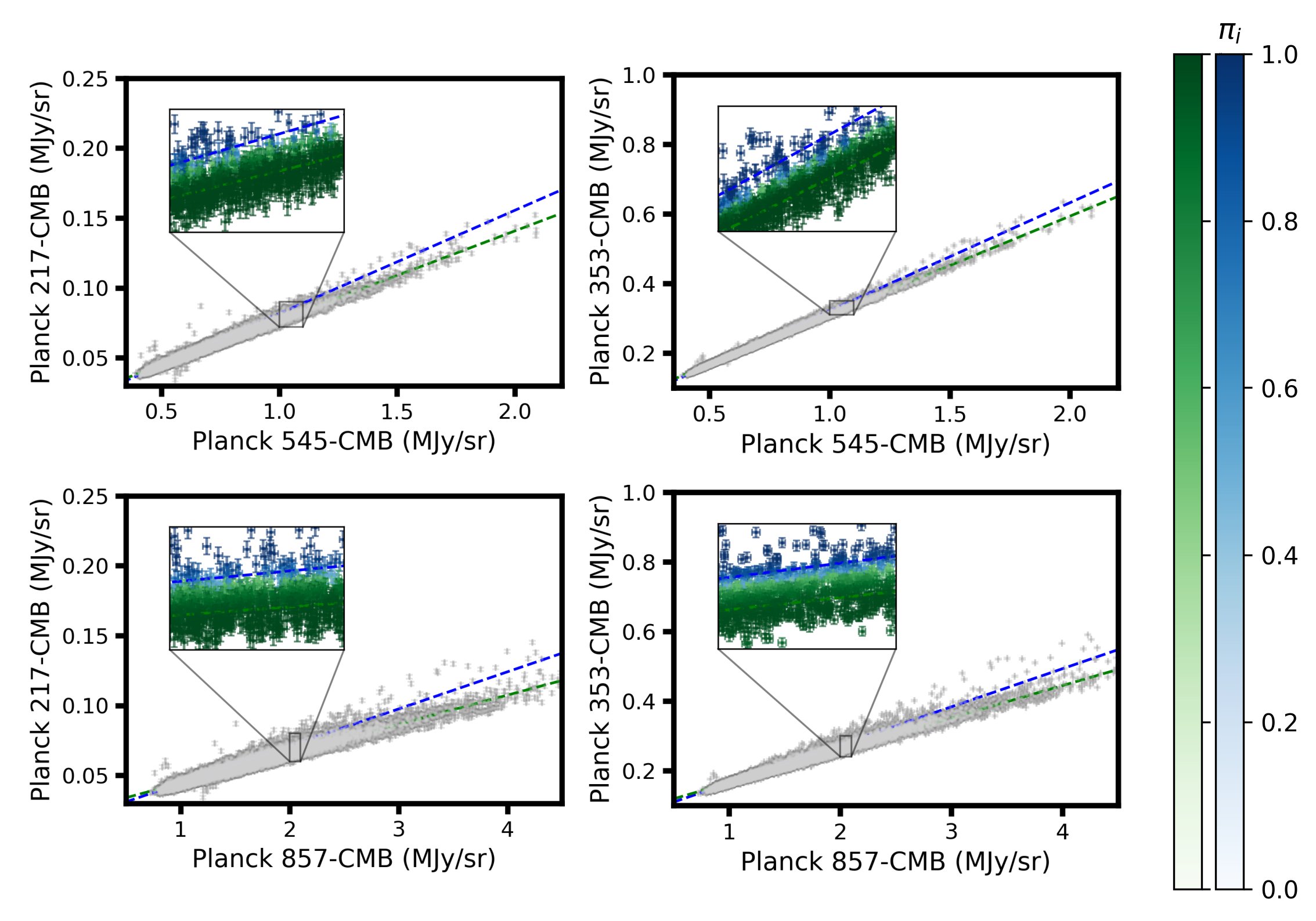
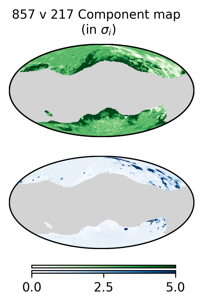
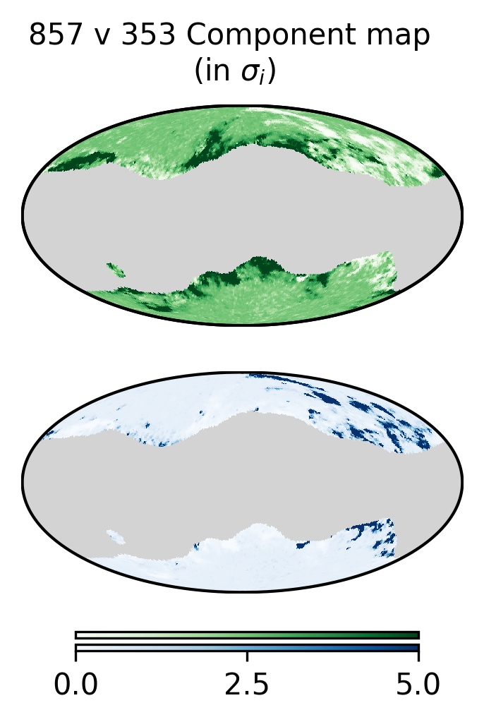
We first conducted this analysis masking the Galactic plane over the cleanest 40% of sky, LR40. We used the full likelihood as described in equation 2 with K=2 populations. Physically, this model corresponds to two dust populations, with a mean frequency scaling $\theta_{k}$, and with some inherent variability inside each population parameterized by $V_{k}$. Therefore, this model expects dust scaling to be a distribution of values rather than a single true population value obscured by statistical noise. The role of modeling $V_{k}$ will be discussed in a future section 7.1. This model allows for miscalibration between frequency pairs and corrects for this by fitting a monopole calibration parameter.

While there is a preference for maximally uninformative priors, mixture models are highly multi-modal and susceptible to being stuck at local extrema (chen_EM_convergence, wu2017convergence). Therefore, in this analysis, we chose largely uninformative priors around realistic values, while not extending infinite support for all values.

The slope was parameterized in angle from the $x$-axis and flat between $[0,\pi/2]$ to not prefer any slope aside from a positive relationship between dust emission. The monopole correction parameter has a truncated Normal distribution $b\sim\mathcal{N}(0,1,\text{low}=-2,\text{high}=2)$ that is practically flat across all relevant values.

We initially used an InvGamma($\epsilon$, $\epsilon$) prior for the variance due to its favorable properties, including (1) being a conjugate prior for a Gaussian, (2) support for infinite positive variance models, and (3) approximate flatness for small $\epsilon$ values. However, we discovered that this prior may lead to pathological fits. Sometimes, the fitted variance is driven by a few outliers and may be many times larger than the variance of the data itself. To address this, we instead selected the prior on the variance to a uniform distribution ranging from 0 to $2\times$ the variance of the underlying data.

Table 2: Fitted parameters for different pairs of analysis in $LR40$ and at $N_{side}=64$. Slopes are presented as $m=\tan(\theta)$, and the variance $V_{k}$ is the variance of the residuals. Note that the variance and slopes are in different units and cannot be directly compared. Instead, these should be compared to the noise levels of table 1 to see the increase in variance relative to the inherent noise level. The expected slopes between frequency pairs obtained with Planck all-sky average values ($\beta_{d},T_{d}$ = 1.53,19.6 K Planck_2018_XI) are [0.356, 0.102, 0.022, 0.287, 0.062] in descending order in the table.

Freq. Pair	Slope		Std. $(MJy/sr)$		Global frac
	$m_{0}$	$m_{1}$	$10^{3}\cdot\sqrt{V_{0}}$	$10^{3}\cdot\sqrt{V_{1}}$	$p_{0}$	$p_{1}$
857$\times$545	0.328	0.362	10.3	17.3	0.67	0.33
857$\times$353	0.093	0.110	5.4	10.2	0.78	0.22
857$\times$217	0.021	0.027	1.8	3.2	0.84	0.16
545$\times$353	0.284	0.310	1.6	3.2	0.85	0.15
545$\times$217	0.064	0.074	0.8	2.2	0.90	0.10

Figure 3 shows the results of the fits to the LR40 data; table 2 summarizes the fitted parameters. The fitted slopes are consistent with our general expectation from Planck all-sky average values $(\beta_{d},T_{d})\sim(1.53,19.6\,K)$. We observe an alternate population over $\sim$15-20% of the analyzed sky at LR40.

The fractional separation between the two population slopes, $(m_{1}-m_{0})/m_{0}$, is more pronounced when the frequencies have a larger difference between them. This is consistent with a dust frequency scaling behavior because if the observed dust is composed of several populations, it becomes advantageous to make comparisons with a lower frequency map. This is due to the longer lever arm it provides, facilitating the differentiation of various SEDs. However, there is a natural trade-off, because lower-frequency maps have lower signal-to-noise. At 857$\times$143 GHz, the identification of multiple populations is not observed because the uncertainty for 143 GHz is larger than the separation of the two populations. For this reason, the analysis with 143 GHz or 100 GHz is not included in table 2.

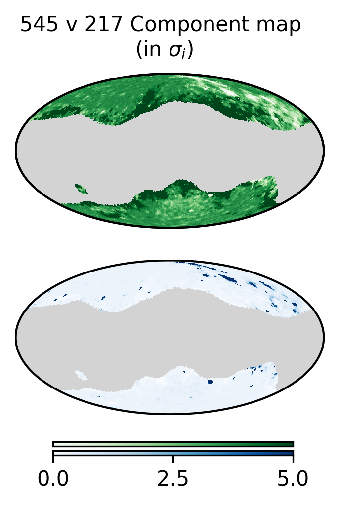
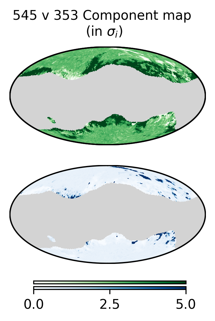
In figure 3, each plot is derived from a pair of HFI maps, one a sub-mm channel (545 GHz,857 GHz), the other a lower frequency map (217 GHz,353 GHz), and every data point has a probability $\pi_{i,k}$ associated with it that describes the probability the point belongs to the $k^{\text{th}}$ population. Because this is treated as a Bernoulli process, each point can be converted to a statistical significance,

$$\sigma_{i,k}=\frac{\pi_{i,k}}{\sqrt{\pi_{i,k}(1-\pi_{i,k})}}$$ (6)

Then, we can transform these pixels back into the spatial domain and plot them in Figure 4. Recall that no spatial information is built into the likelihood in equation 2. Nevertheless, each population that is fitted shows a coherent spatial structure. We observe a primary dust population in green, with high confidence, originating from dusty regions near the Galactic plane, and we identify isolated blue dust clouds that indicate the presence of a distinct population.

5.1 Comparison to known sources

We can compare our identified dust population to a dust extinction map. One such map is the Draine-Li 2007 dust extinction map. A visual comparison between this map and our most sensitive cross, 857$\times$353 GHz, only shows a weak correlation. While some of the denser dust regions show up in the dust population mask, our analysis primarily identifies clouds on the eastward side of the Galactic plane. A simple Pearson correlation coefficient between a dust extinction map and our own analysis, over LR40, puts a correlation of $\rho=0.32$. Clearly, dust density itself cannot be a good explanation for the observed population distribution.

Polarized radio loops are the largest structures in the sky and cause extended filamentary structures extending from the Galactic Plane (Vidal_2015). They are believed to be caused by supernovae remnants locally, and while brightest at radio frequencies from synchrotron radiation, they are also visible in the mm and sub-mm (Liu_2014). Indeed, the largest loops: I, II, III are clearly missing in the identified dust population. However, smaller more localized bubbles may be responsible for some of the identified structures juan_superbubble. A more systematic and careful comparison is warranted but beyond the scope of this paper.

6 Analysis over the Spider Region

Figure 5: Analysis of the dust population over the Spider observation region: a region in the Southern sky at Galactic latitudes greater than $|b|>20^{\circ}$. The leftmost panel shows Planck’s 857 GHz map, which is a sensitive tracer of diffuse dust emission, over this region. The plots on the right show the identification of the dust populations, plotted as the difference $(\sigma_{1}-\sigma_{0})$ for brevity. The four panel plot displays the analysis conducted with Planck 857 GHz and its corresponding frequency pair indicated above or below each subplot. With high confidence, we identify two populations of dust using any of the four input maps (Planck 217,353, and 545 GHz and IRAS 100 $\mu m$). We observe coherent dust clouds (in blue) that are interspersed between filamentary structures (in green). A visual comparison of the cloud structures with the dust intensity on the left shows little correlation between the two maps.

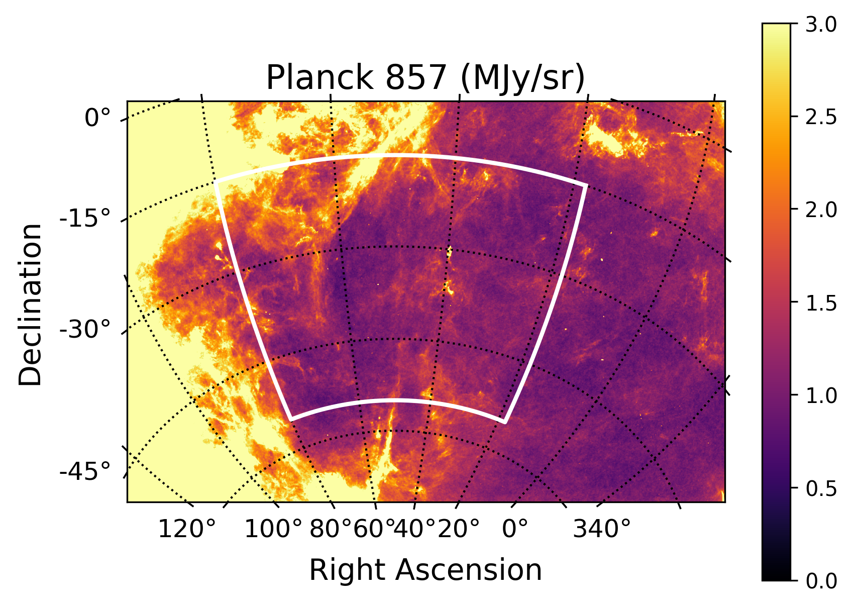
The investigation of dust properties in high-Galactic latitudes holds considerable significance in the context of CMB studies. The conventional approach has focused on observing smaller sky areas, selected for reduced contamination from foreground sources (spider_bmode, bicep_2018, Adachi_2022). We repeat this analysis over the Spider region to identify if we can detect multi-population dust in this region: a high-Galactic latitude region $(|b|>20^{\circ})$ in the southern hemisphere comprised of $\sim$5% of the full sky. This analysis is limited to dust intensity rather than polarization. Indeed, regions that are bright in polarization typically are the edges of dust clouds, where the magnetic field environments are more orderly than in the dense inner regions of clouds that are optically deep in intensity (planckXIX2015). However, the detection of a multi-population dust model in intensity would reveal that the foregrounds in this region are more complex than commonly modeled.

The preprocessing pipeline is identical to that of section 4, except the results presented here are at higher resolution $N_{side}=128$ and includes the ISSA reprocessing of the IRAS 100 $\mu$m data (ISSA ). The CMB is not subtracted from this map, as it’s expected to be negligible at this frequency. Additionally, this map is smoothed to a common 10 arcmin resolution, which necessitates careful handling to avoid artifacts in the Spider region. ISSA maps provide coverage for 98% of the sky, with the missing 2% region coming close to the Spider observation region. The missing region can be masked with a 3.75 deg apodization, chosen optimally to minimize ringing while avoiding masking the region of interest itself. Noise in the ISSA map is complex, although a uniform noise estimate has been tabulated as 0.07  MJy/sr$\pm$ 0.03 MJy/sr (ISSA, Miville_Deschenes_2005). Out of caution, we adopt a noise level estimate that is 50% larger than the quoted value, 0.105 MJy/sr, uniformly across all pixels in the region.

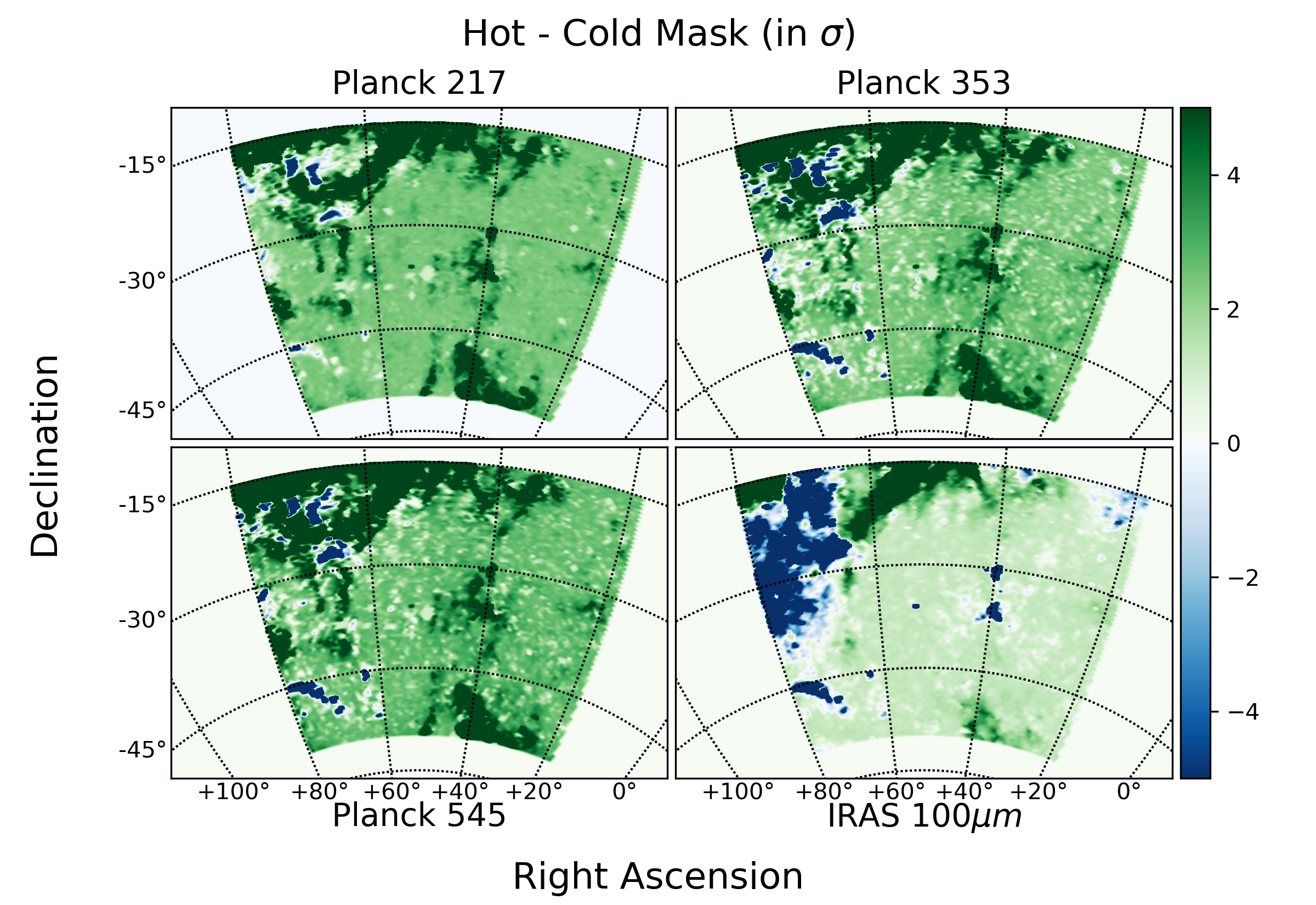
For this analysis, we use the same dust modeling as in section 5, where we fit two dust populations with a mean and variance for each. A summary of the results is shown in figure 5 where four different frequency pairs are considered: Planck 217, 353, and 545 GHz and IRAS $100\,\mu m$, all relative to Planck 857 GHz.

The fitted population fraction for the alternative model is $p_{1}=0.12,0.15,0.12,0.34$, respectively, with $\sigma(p_{1})=0.01$ across all frequency pairs. In every case examined, we consistently observe coherent and filamentary structures across all pairs included in this analysis.

The comparison of Planck 857 GHz with Planck 545 GHz is the most challenging due to the smallest frequency separation and, therefore, the most similar slope between populations. Indeed, in the analysis with 545 GHz, the fit prefers a very similar slope between the two populations $m_{0}\approx m_{1}$ with a substantially wider variance $V_{1}\gg V_{0}$ which captures many of the outlier dust points. Other analysis crosses instead distinguish themselves in $m_{k}$.

For that reason, only a few points distinguish themselves in the cross with 545 GHz. Conversely, IRAS has the longest lever arm and also contains the most different spatial arrangement. Specifically, the shape of the dust cloud is different in the upper left region, and there is a disagreement in population assignment in the central part of the region. ISSA has its own residual artifacts in its map, which differ from those of Planck’s. Therefore, identifying common dust populations strengthens the case for spatially separated dust populations in this region.

We thus demonstrate that even the relatively clean Spider region, known to be composed mainly of diffuse, non-turbulent dust (planck_XLIV), contains statistically detectable dust populations in intensity. While we expect the populations responsible for polarized mm-emission to differ from those that are bright in intensity, the existence of multiple dust populations in intensity suggests that dust is more complicated than commonly modeled.

7 Robustness to Analysis Choices

The likelihood function plays a central role in Bayesian parameter estimation. Therefore, it is crucial to check the appropriateness of the likelihood for the data at hand. In this section, we explore different likelihood choices to test the robustness of the conclusions.

7.1 Modeling dust without inherent scatter, $V_{k}=0$

(a)

(b)

(c)

(d)

(e)

Figure 6: Investigating alternate analysis choices and their effect on dust populations. (a) Reference figure as shown in figure 4 for the basis of comparison. (b) Likelihood model of dust composed of discrete populations with no intrinsic variations, $V_{k}=0$. The plotted results include a two-sided CDF factor to suppress points far away from the model. All structures disappear with this additional confidence factor. Therefore, the data points are distributed further away than if noise was the sole factor for variations from the mean. (c) Instead of a CDF factor, a beam smoothing factor with a FWHM = 1deg is applied to the $\pi_{i}$ to suppress noise. Coherent structures remain, suggesting that spatial information may allow the separation of even more components. (d) Filtered maps that remove large-scale artifacts in the map. The variance is fit $V_{k}$, while the monopole offset is not needed $(b_{k}=0)$. We see a similar spatial arrangement of our two populations, indicating that large-scale residual effects, primarily the residual solar dipole, do not inadvertently influence our identification of two populations. (e) No hyperparameter prior $p_{A}$. In this configuration, $\pi_{i}$ is drawn from a uniform distribution from 0 to 1.

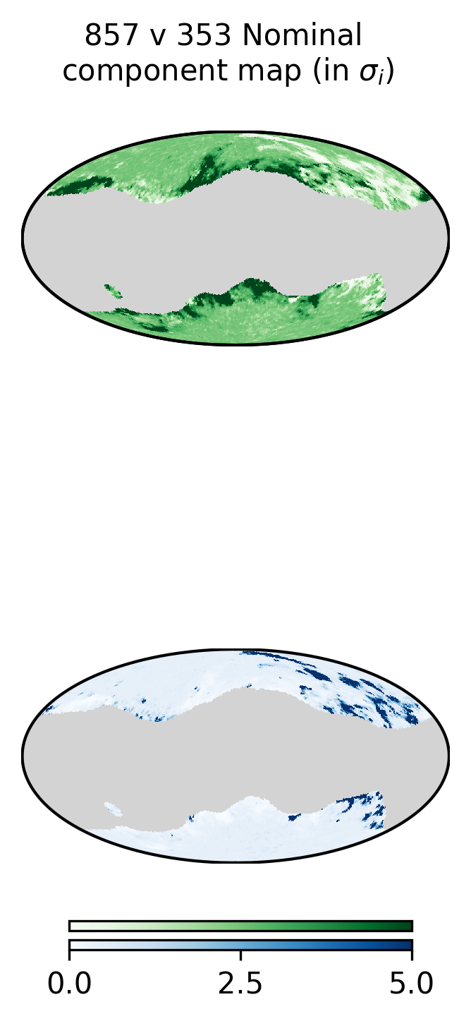
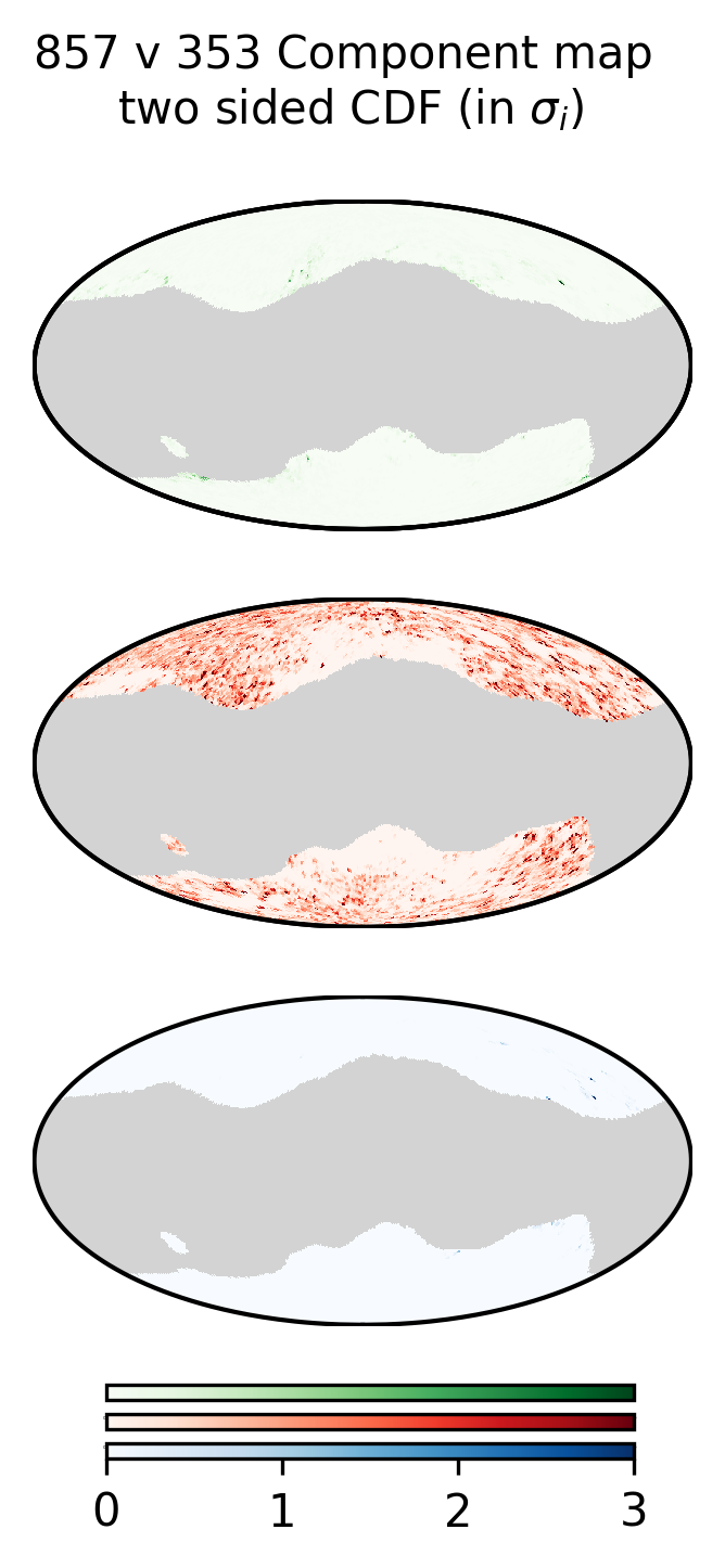
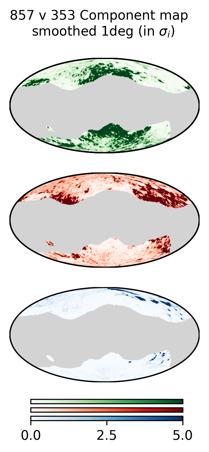
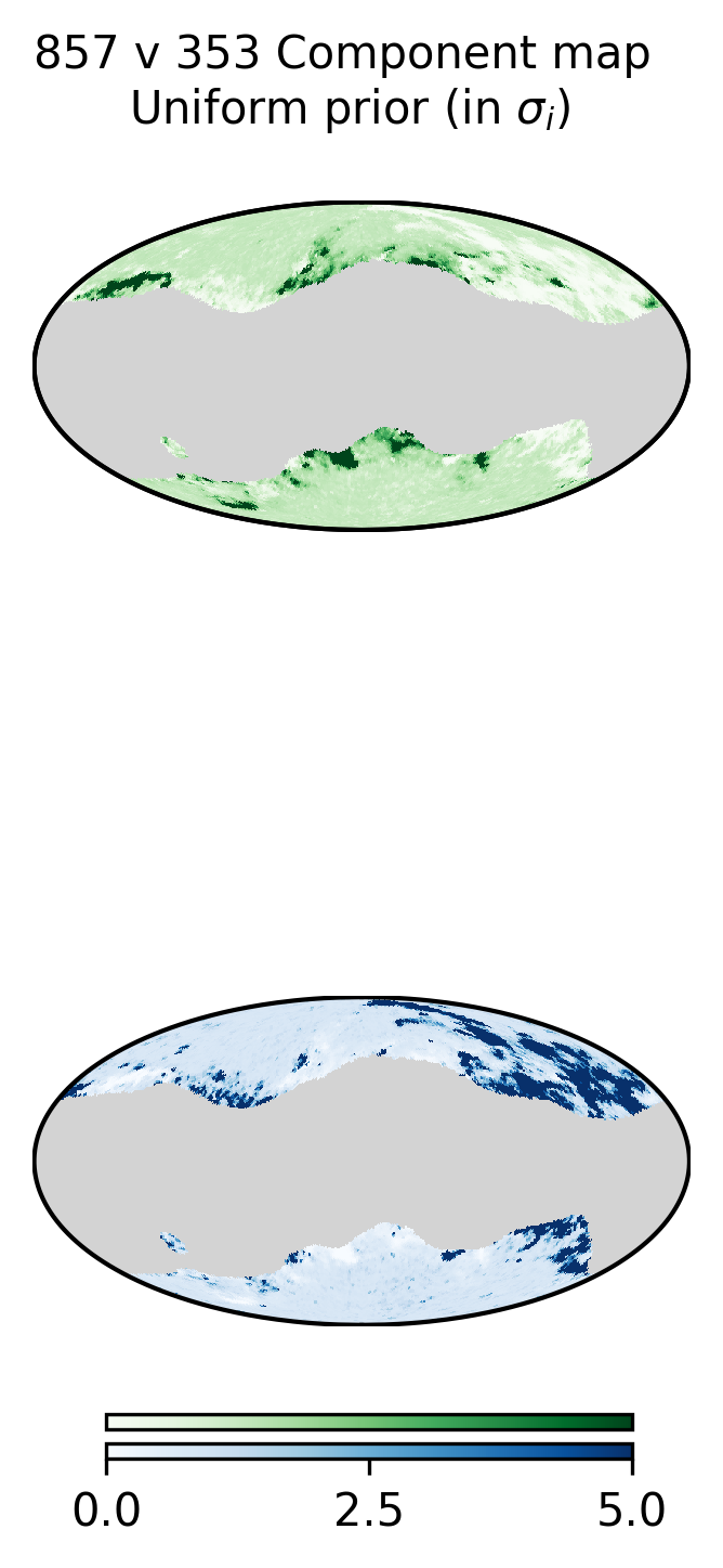
In section 5, our likelihood model incorporates a term denoted as $V_{k}$, representing the variance specific to each population. This has a physical interpretation within the model: we are studying different dust populations, and these populations are generated through a process characterized by an average scaling value, $\theta_{k}$, with inherent variations about that mean value captured by $V_{k}$.

In this section, our objective is to investigate whether the data can be accurately represented using only a scaling value, $\theta_{k}$, with a monopole offset. In this model, any observed variance should be attributed solely to measurement noise.

To account for the variation in data points, we find that the data prefers a fit with three slopes. In figure 6(b), these are sorted from shallowest (green), middle (red), to steepest (blue). When we look at our most significant dust cross, 857$\times$353 GHz, we have three distinct dust populations, with fitted population fractions of {0.47, 0.46, 0.07} from the shallowest to the steepest slope. These proportions remain true for several different frequency crosses.

In cases where there is insufficient statistical power to fit three populations and instead, two populations are fit, the likelihood analysis prefers to lump populations 0 and 1 together and still distinguish population 2 separately. This is evident in the cross 545$\times$217 GHz.

In the likelihood analysis, each pixel is assigned a probability $\pi_{i}$ of belonging to one of K populations. The probability is determined by its distance to each population based on the likelihood ratio: $\pi_{i,k}=\mathcal{L}_{i}(k)/\sum_{k}\mathcal{L}_{i}$.

The likelihood function, comprised of a sum of Gaussians, makes the likelihood ratio highly sensitive to the distance of each data point from its nearest population.

Within this framework, the impact of statistical noise inadvertently magnifies. Points exhibiting fluctuations near the population boundaries draw exponentially closer to one population over another, leading to $\pi_{i}$ assignments that are overly confident.

$$cdf_{i}=\left(\int_{-\infty}^{-|\Delta|}+\int_{|\Delta|}^{\infty}\right)\mathcal{N}(0,\sigma)$$ (7)

To accurately assess the likelihood of a data point belonging to a particular population, we employ a two-part measure. We combine the likelihood ratio, $\pi_{i}$, with a confidence score (eq. 7) based on a two-sided cumulative distribution value. This distribution is Normal with mean 0 and a width equal to the statistical uncertainty of point $i$. This confidence score reflects the point’s proximity to the population and down-weights points if they are close to a likelihood boundary.

We convert the probability to a $\sigma$-level by treating each pixel as a Bernoulli process,

$$\sigma_{i}=\frac{\pi_{i}\cdot\text{cdf}_{i}}{\sqrt{\pi_{i}\cdot\text{cdf}_{i}\cdot(1-\pi_{i}\cdot\text{cdf}_{i})}}$$ (8)

Figure 6(b) plots the $\sigma_{i}$ back into spatial coordinates. However, our inclusion of the cdf factor eliminates all visible structure for the two extremum populations. Mathematically, this implies the variability within each population exceeds the quoted uncertainties. This has a physical interpretation in that dust must not be generated from a physical process with a “true” set of ($\beta_{d},T_{d}$) values. Even in the absence of measurement noise, the expectation is a natural variation in dust parameters ($\beta_{d},T_{d}$). As a result, the likelihood 2 with $V_{k}=0$ cannot accurately capture the physics of this observed set of data.

7.2 Using spatial information

While the likelihood with $V_{k}=0$ may not capture all the nuances of the data, it does offer a valuable basis for further investigation.

Rather than introduce a confidence factor $cdf_{i}$, we can instead make use of spatial arrangements of pixels to suppress the effects of noise. When multiple neighboring pixels agree on a population, then this consensus strengthens our confidence in the correctness of the assignment. Alternatively, if neighboring pixels conflict, we should suppress the assignment.

A simple way to implement this a posteriori is to apply a smoothing factor on the probability map $\pi$. We smooth the map with a symmetric Gaussian beam, and then calculate the $\sigma$-significance in the same way (eq 6).

Figure 6(c) shows the results of our most sensitive cross, 857$\times$353 GHz, when smoothed with a 1-degree beam. From the top to the bottom, we see dust emission centered around the Galactic plane, followed by more diffuse Galactic emission at the edges of the Galaxy closer to the poles. The last population is isolated cloud structures that deviate from the general dust population.

This analysis reveals insights about the arrangement of dust data points in the scatterplot (Fig. 3). Notably, the stratification of pixels in the scatterplot space holds physical significance. Points with lesser slopes come from the brightest regions of the Galaxy, while points with greater slopes come from more diffuse regions of the galaxy.

This analysis suggests that incorporating spatial information into the likelihood equation could potentially yield additional insights into dust populations. Such an extension would require us to encode the spatial relationship between pixels in the likelihood. Neighboring pixels may collectively indicate the presence of an alternate population, even if individual pixels lack sufficient statistical significance for identification. Such an analysis would be a substantial increase in modeling complexity. In intensity, we have high-frequency data with strong signal-to-noise ratio, allowing us to differentiate points without relying on spatial information. Instead, this extension could prove valuable in the study of polarized foregrounds. However, it falls outside the scope of this paper to introduce spatial modeling.

7.3 Removing dipole residuals with harmonic space filters

There are several challenges with analyzing native Planck maps. Planck maps contain an irreducible zero-level offset. The monopole offset has physical sources, including cosmic infrared background and zodiacal emission (planck_III_2018). Typically this offset is adjusted based on tracers from other datasets, such as HI (planck_III_2018). The monopole offset

Additionally, the Planck maps contain residual artifacts from the Solar dipole: the motion of the Solar System relative to the rest frame of the CMB. The major effect of residual dipole occurs at $\ell=1$. However, relativistic corrections will leak into smaller scales $\ell>1$ (planck_VIII_2015).

While the zero-level offset is naturally handled in the likelihood for equation 2, a residual dipole in the map has no natural way to be built into the likelihood and, therefore, no way to correct for its effect.

The approach in this section is to circumvent these issues by filtering the maps to eliminate large scale features and fit only dust anisotropies. We apply an aggressive window function that removes all power below $\ell\leq 8$, effectively eliminating all possible large-scale dipole residuals. To reduce the impact of undesired ringing, we choose a cosine apodization around $\ell=20$ to smoothly taper the filter’s response function.

$$W(\ell)=\begin{cases}0\qquad&\text{ if }\ell\leq 8,\\ 0.5\left(1-\cos\left(\frac{2\pi(\ell-8)}{50}\right)\right)\qquad&\text{if }8<\ell\leq 33,\\ 1&\text{if }\ell>33\end{cases}$$ (9)

Additionally, we take precautions to prevent bright Galactic plane emissions from causing unwanted leakage into the rest of the map, which would inadvertently bias our analysis. For this reason, we apply the filter to the LR60 masked region, ensuring minimal ringing in LR40, the specific region of interest for this analysis.

With these preprocessing steps, no offsets are needed in equation 2; therefore, we set $b_{k}=0$ for all $K$ populations. We include $V_{k}$ in this version in order to compare it to our nominal case.

We fit the filtered maps with $K=2$ populations, resulting in two distinct slopes. Figure 6(d) visualizes the results in the spatial domain. We see a spatial arrangement of pixels similar to the unfiltered analysis: A dominant diffuse population alongside an alternate population localized to specific clouds. This is consistent with the analysis in section 5; therefore, we believe that large-scale residual artifacts in Planck cannot be the origin of these SED variations.

7.4 Removing hyperparameter $p_{K}$

In section 3, we demonstrated the necessity of the hyperparameter $p_{A}$ for $q_{i}\sim\text{BetaBinom}(n=1,\alpha=p_{A},\beta=1-p_{A})$ to ensure an unbiased recovery of our simulated inputs. However, in this section, we intentionally omit the hyperparameter to observe the impact on this analysis. In this configuration, $q_{i}\sim\text{BetaBinom}(n=1,\alpha=1,\beta=1)$. Effectively, we first draw $\pi_{i,A}$ from a Uniform(0,1) distribution. Then, $q_{i}$ is drawn from a Bernoulli distribution with $p=\pi_{i,A}$.

The outcomes of this configuration, as depicted in Fig. 6(e), reveal a similar spatial arrangement of pixels. The similarity arises because data points that show substantial separation between two populations possess sufficient statistical power to remain largely unaffected by the absence of the prior. Indeed, a simple calculation of the Pearson correlation coefficient between the nominal case and this case is 0.88. The scatterplot of $p_{i}$ between both scenarios demonstrates a monotonic but non-linear relationship. Therefore, despite a large difference in analysis choice, we maintain a relatively high correlation coefficient.

However, points that fall statistically in-between populations are instead heavily influenced by the choice of prior. In this case, points are assigned evenly between two populations, causing the global slopes to converge and leading to an over-identification of the less numerous blue population. This behavior is evident in the simulations (fig. 2) where there is a substantial bias in the globally fitted slope and a greater assignment of the alternate population. On the data, the alternate population $\geq 3\sigma$ expands substantially from 6% to 15%.

While a uniform distribution is often thought to be uninformative, it’s important to note that its mean is fixed at 0.5. This fixed mean influences $\pi_{i,A}$ to tend towards larger values compared to a scenario where a hyperparameter $p_{A}$ is allowed to adapt the mean based on what is preferred by the data. Consequently, using a uniform prior leads to a less conservative identification of an alternate population. For this reason, and because it fails to recover inputs on simulations, we opt not to use a uniform prior on $\pi_{i,A}$ for this analysis.

8 Bayesian Evidence for the Models

The previous sections have demonstrated there is a lot of choice in the models we can fit to our data. Indeed, more components will always fit the data better and return a higher likelihood value, but at the cost of model complexity. To select the correct model to fit, we ask which of the models has the highest marginal likelihood, or the highest Bayesian evidence.

Calculation of Bayesian evidence is computationally expensive and requires a sum (of eq 2) over $K^{N}$ states of $q_{i}$. This is simply intractable for our pixelization and sky area. Instead, we can perform an analytical trick to simplify the calculation of the marginal likelihood. Following the method of hogg_likelihood, each $q_{i}$ has K possible states with probability $\{p_{1},\cdots p_{k}\}$ so the likelihood, marginalized over $q_{i}$, can instead be written as a sum of states,

$$\mathcal{L}(\theta_{k},b_{k},V_{k},p_{k})=\prod_{i}\sum_{k}\left[\frac{p_{k}}{\sqrt{2\pi(\Sigma_{k,i}+V_{k})}}\exp\left(-\frac{\Delta_{k,i}^{2}}{2(\Sigma_{k,i}+V_{k})}\right)\right]\\$$ (10)

where now the likelihood only has $4K-1$ parameters.

We use the nested sampler dynesty (dynesty_citation, dynesty_software) to perform this calculation with results in table 3. The statistical and sampling uncertainty for all the quoted values is subdominant to the significant figures in the table.

The preferred model, for the majority of the crosses, is a two-population ($K=2$) model that include an additional variance term $V_{k}$. For this reason, the quoted results in section 5 are those of this analysis. However, as we go to lower frequency crosses, the signal-to-noise is lower on dust and simpler models are adequate to explain the variations in the data. For $545\times 217$, a multi-population dust model with no additional variance $(V_{k}=0)$ has the highest evidence.

One could combine all datasets Planck 100-857 GHz and IRAS 100 $\mu$m and construct a multi-variate likelihood to fit them simultaneously. Such an approach would not significantly increase the number of fitted parameters, because the parameter $q_{i}$ is associated with each spatial pixel and would not scale with the number of inputs. However, since our pairwise analysis shows a clear distinction between the two populations, we have chosen not to pursue this extension at this time.

Table 3: Calculation of marginal likelihood over $LR40$ with $N_{side}=64$ using two different models: inc $V_{k}$ as described in section 5 and $V_{k}=0$ as described in section 7.1. All values of marginal likelihood are in $\log_{10}$ units. The highest evidence values are bolded. The highlighted blue background provides a qualitative comparison of the log marginal likelihood values in relation to the highest value in the row.

	Inc. $V_{k}$		$V_{k}=0$
Frequency pair	$K=1$	$K=2$	$K=1$	$K=2$	$K=3$
857$\times$545 GHz	1.3E4	1.4E4	-3.7E5	-1.3E5	-7.5E4
857$\times$353 GHz	4.0E3	5.4E3	-5.0E4	-1.4E4	-5.6E3
857$\times$217 GHz	7.5E2	1.7E3	-9.9E3	-1.6E3	-6.4E2
545$\times$353 GHz	1.1E4	1.3E4	7.4E3	1.2E4	1.2E4
545$\times$217 GHz	4.5E3	4.6E3	4.7E3	4.9E3	5.0E3

9 Inferred Galactic Dust Properties

Figure 7: Inferred dust properties from the two populations as shown in figure 4. The mask chosen was LR40, constructed from 857$\times$353 GHz, applied to all frequencies Planck HFI and IRAS 100 $\mu m$, and only high confidence pixels were included in the analysis with $\geq 3\sigma$ confidence in assignment of population. On the left, we have the best-fit dust parameters $(\beta_{d},T_{d})$. Plotted in black is Planck’s 2015 thermal dust model from the Commander pipeline: distribution of $(\beta_{d},T_{d})$ values masked to LR40. The two populations here have overlapping contours only at the $\sim 2.5\sigma$ with the alternate population (in blue) at fixed $\beta_{d}$, preferring a colder $T_{d}$, or at fixed $T_{d}$, preferring a shallower $\beta_{d}$. This indicates that there are physical differences between the two populations. On the right, the SED model is compared to the measured flux ratios with their full bandpass corrections. The alternate population, the blue points, are shifted in frequency purely for visual separation of the two populations. The SED model accurately captures the measurements at all frequencies.

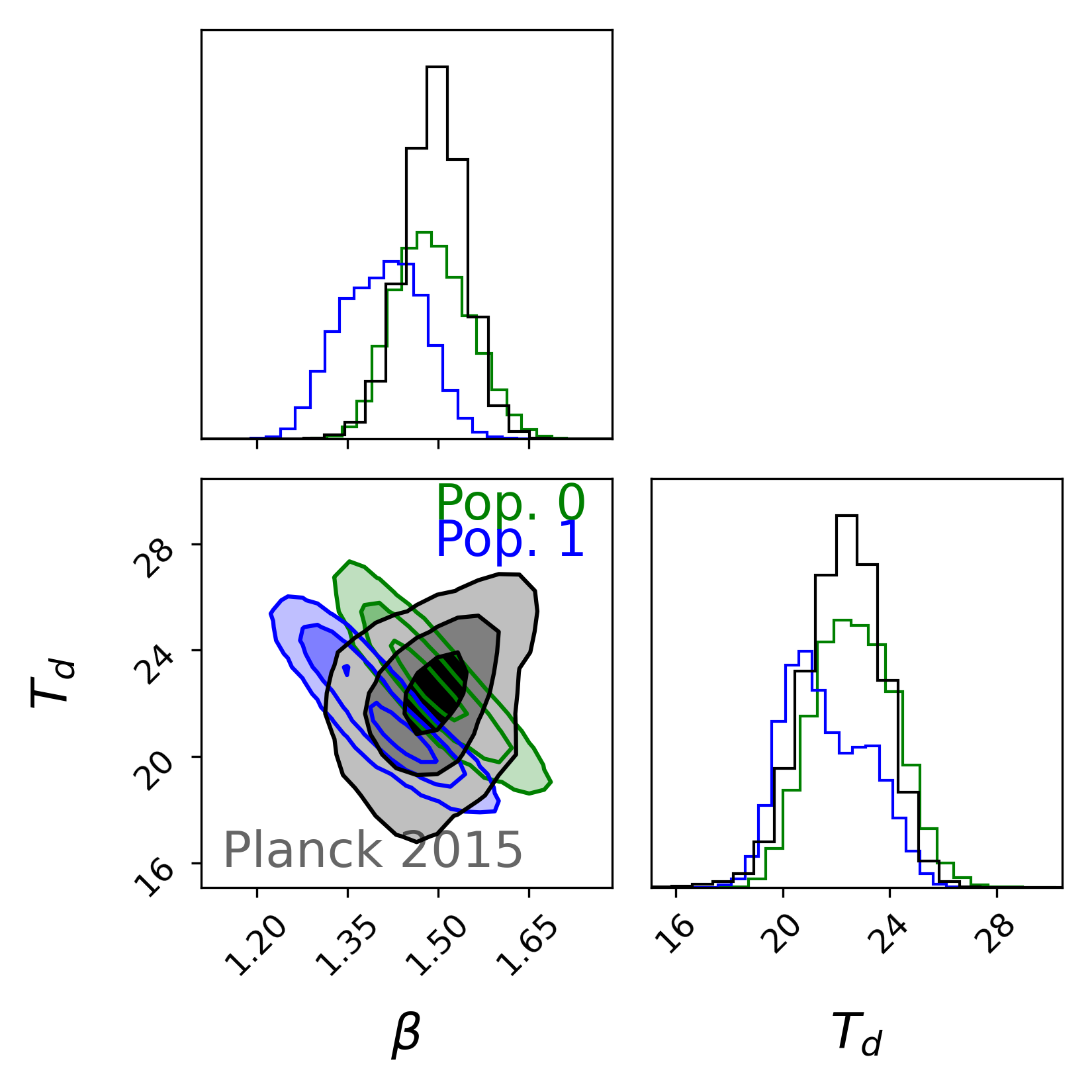
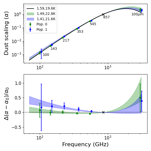
Having identified the two dust populations, we can further infer the properties of each. We construct a mask to optimally separate the two populations. We use a 857$\times$353 GHz $\sigma$-map, as shown in figure 4, and include only high-confidence pixels with $\geq 3\sigma$ confidence in the assignment of population. We apply this mask to all frequencies, Planck HFI and IRAS 100 $\mu m$. Then, we subtract a previously fitted monopole correction term and calculate the flux ratio $\alpha$ relative to our reference frequency for each frequency and population.

The $\alpha$’s are shown on the right side of figure 10, where the uncertainties signify a $1\sigma$ variation in the population. These distributions are inherently non-Gaussian. To analyze them, we perform a Gaussian kernel density estimate (KDE), denoted by $\alpha_{kde}$, using Scott’s rule for bandwidth estimation (scotts_rule, scipy).

The flux ratio can be related to a standard dust SED by the following definition:

$$\alpha(\nu,\beta_{d},T_{D})=\frac{I(\nu)}{I(\nu_{0})}=\frac{b_{c}(\nu)}{b_{c}(\nu_{0})}\left(\frac{\nu}{\nu_{0}}\right)^{\beta_{d}}\frac{B(\nu,T_{d})}{B(\nu_{0},T_{d})},$$ (11)

where $\beta_{d}$ is the spectral index of dust, $B(\nu,T_{d})$ is the Planck blackbody emission at temperature $T_{d}$, $\nu_{0}$ is the reference frequency 857 GHz, and $b_{c}(\nu)$ is a bandpass correction for map $\nu$ as defined by the reciprocal of equation 35 in planck2013_spectralresponse. The full spectral bandpass for Planck and IRAS are both used for the color correction. Fitting flux ratios instead of fluxes directly allows us to avoid fitting for the dust optical depth, as it is not a fundamental property of dust physics.

We construct a likelihood function based on the Gaussian KDE of $\alpha$,

$$\log\mathcal{L}(\beta_{d},T_{d})=\sum_{\nu}^{\text{ HFI, {IRAS} 100}}\log\alpha_{kde}(\alpha(\nu,\beta_{d},T_{d}))$$ (12)

To find the best-fit dust parameters, we maximize the likelihood with respect to $\beta_{d},T_{d}$. We choose uniform flat priors for $\beta_{d},T_{d}$. The fits are performed with The marginal parameters show a substantial overlap between the two populations because of the high degeneracy between $\beta_d-T_d$.Intuitively, this degeneracy naturally occurs because both $\beta_d$ and $T_d$ can influence the peak of the blackbody function. An underestimation of $\beta_d$ leads to a more emissive Rayleigh-Jeans portion of the curve and pulls the peak towards lower frequencies. To compensate, a hotter dust temperature pushes the peak back towards higher frequencies (\cite{Chen_2016}).This anti-correlation has been observed in other analyses (\cite{planck_XIV_2014}), and \cite{Shetty_2009} has attributed this anti-correlation to measurement uncertainty. While a hierarchical Bayesian model has been demonstrated to mitigate this effect (\cite{Kelly_2012}), this modeling extension was not pursued in this analysis.The 2D likelihood contours show separation of the two populations at the mutual $\sim$$2.5\sigma$ level. These values of $\beta_d, T_d$ accurately reproduce the observed flux ratios at all frequencies, as evident on the right side of figure \ref{fig:dust_inference}. This implies that we have distinct spatially separated dust populations, with each population being effectively characterized by a single-component SED.It is important to remember that the uncertainties in these parameter estimations represent the variability of the population rather than statistical uncertainty on the populations.\section{Conclusion}\label{sec:conclusion}We have developed a powerful technique for spatially separating dust populations based on Gaussian mixture models using HMC methods. We constructed a GMM likelihood function with no inherent spatial information. The analysis results provide, for each pixel $i$, a probability $\pi_{i,k}$ that it belongs to population $k$.We have shown it is highly accurate at recovering input parameters, even in the limit where populations are heavily mixed.We then applied this method to the \Planck HFI intensity maps to identify pixels that statistically deviate from a main population.When we show the arrangement of pixels, clear patterns emerge in the map, showing distinctive regions where an alternate population is favored.We tested this conclusion to many different analysis choices: (1) in section \ref{sec:lr40_analysis}, we used entirely independent frequency crosses, i.e., 545$\times$217\,GHz and 857$\times$353\,GHz, and confirmed the presence of two dust populations with similar spatial arrangements, (2) in section \ref{sec:spider_analysis}, we changed the masked area and showed that multiple populations are detectable even in cleaner sky regions with more diffuse dust, (3) in section \ref{sec:analysis_choices}, we explored the sensitivity of the likelihood model ($V_k = 0$) and confirmed that this effect is still observed when the likelihood is modified, (4) in section \ref{sec:filter}, we repeated the analysis on filtered maps that are designed to remove residual large-scale artifacts in the \Planck maps and confirmed that this effect is not attributable to such artifacts.Then, in section \ref{sec:evidence}, we calculate the Bayesian evidence to see which of these analysis choices are favored. The most favored model for the majority of the crosses is a two-population dust model with inherent variability of each population $V_k > 0$. As the signal to noise on dust drops, so does the Bayesian evidence for this effect. Indeed, for the 545v217 cross, we compute the highest Bayesian evidence for a three-population dust with no variability ($V_k = 0$).We also provide a promising path for improving this analysis. All datasets could be combined and simultaneously fit with a multi-variate likelihood. We expect such an extension to be computationally feasible since the dominant contributor to variable count does not scale with the number of input maps. Additionally, in this work, we excluded spatial information in the likelihood in due caution to be unbiased in population recovery. Combining statistical power of neighboring pixels can provide additional statistical weight that is otherwise unused in this analysis, potentially revealing further insights about the variability of dust populations.This analysis reveals that the nature of dust is more complex than can be adequately described by a single-component modified blackbody model. Instead, our findings strongly suggest that a spatially varying two-population dust model better aligns with the observed data. Identifying an alternate population and its distribution can provide further insights into the nature and structures of Galactic dust.With a two-population dust, CMB component separation becomes a substantially more challenging task.Failure to correctly account for the spectral variations can lead to residual contamination.To effectively distinguish these dust populations, we need high-fidelity, high-frequency measurements.Indeed, this analysis would not have been possible without using intensity measurements from \Planck 545 and 857\,GHz.A similar understanding of dust polarization remains an open question. Polarized maps do not exist at comparable high frequencies.Further insights into the nature of polarized dust emission necessitate higher sensitivity data, particularly in the sub-mm and far-infrared ranges.These measurements are accessible only through next-generation sub-orbital and orbital experiments.In conclusion, this analysis is another step in understanding the complexity of Galactic foreground emission. The improvement of statistical tools, in conjunction with data from \Planck’s␣highest␣frequency␣channels,␣has␣enabled␣us␣to␣differentiate␣between␣multiple␣un-polarized␣dust␣populations.␣Increased␣instrumental␣sensitivity␣of␣next-generation␣CMB␣experiments␣will␣lead␣to␣data␣that␣is␣more␣discerning.␣Simple␣foreground␣models␣may␣no␣longer␣suffice.␣A␣continued␣refinement␣of␣foreground␣models␣is␣essential␣to␣enhance␣our␣ability␣to␣extract␣ever-tighter␣cosmological␣constraints␣from␣the␣CMB.\begin{acknowledgements}This␣research␣is␣supported␣by␣the␣National␣Aeronautics␣and␣Space␣Administration␣grant␣␣NNX17AC55G.We␣want␣to␣express␣our␣thanks␣to␣Elle␣Shaw.␣Her␣careful␣review␣and␣helpful␣editorial␣suggestions␣significantly␣improved␣our␣work.␣Many␣of␣the␣results␣in␣this␣paper␣have␣been␣derived␣using␣the␣HEALPix␣package␣(\cite{HealPix}).␣Computations␣were␣performed␣on␣the␣Niagara␣supercomputer␣at␣the␣SciNet␣HPC␣Consortium.␣SciNet␣is␣funded␣by␣Innovation,␣Science␣and␣Economic␣Development␣Canada;␣the␣Digital␣Research␣Alliance␣of␣Canada;␣the␣Ontario␣Research␣Fund:␣Research␣Excellence;␣and␣the␣University␣of␣Toronto␣(\cite{Niagara}).\end{acknowledgements}\FloatBarrier\appendix\input{appendix}\label{sec:appendix_derivation}\FloatBarrier\bibliography{references}{}\bibliographystyle{aasjournal}\end{document}’