Evaluation of Bjorken polarised sum rule with a renormalon-motivated approach

Abstract

We use the known renormalon structure of Bjorken polarised sum rule (BSR) ${\overline{\Gamma}}_{1}^{p-n}(Q^{2})$ to evaluate the leading-twist part of that quantity. In addition, we include $D=2$ and $D=4$ Operator Product Expansion (OPE) terms and fit this expression to available experimental data for inelastic BSR. Since we use perturbative QCD (pQCD) coupling, which fails at low squared spacelike momenta $Q^{2}\lesssim 1\ {\rm GeV}^{2}$ due to Landau singularities, the fit is performed for $Q^{2}\geq Q^{2}_{\rm min}$ where $Q^{2}_{\rm min}\approx(1.7\pm 0.3)\ {\rm GeV}^{2}$. Due to large BSR experimental uncertainties, the extracted value of the pQCD coupling has very large uncertainties, especially when $Q^{2}_{\rm min}$ is varied. However, when we fix the pQCD coupling to the known world average values, the $D=2$ and $D=4$ residue parameters can be determined within large but reasonable uncertainties.

I Introduction

The polarised Bjorken sum rule (BSR) ${\Gamma}_{1}^{p-n}(Q^{2})$ BjorkenSR is the difference of the first moment of the spin-dependent structure functions of proton and neutron. Due to its spacelike and isovector nature it has a relatively simple form of OPE. Experiments with scattering of polarised leptons on polarised targets give us measured values of the inelastic BSR ${\overline{\Gamma}}_{1}^{p-n}(Q^{2})$. They have been performed over a large interval of $Q^{2}$, $0.02\ {\rm GeV}^{2}<Q^{2}<5\ {\rm GeV}^{2}$, at CERN CERN , DESY DESY , SLAC SLAC , and at various experiments at the Jefferson Lab JeffL1 ; JeffL2 ; JeffL3 ; JeffL4 ; JeffL5 . These data points still have significant statistical and systematic uncertainties.

The theoretical evaluation of the inelastic BSR ${\overline{\Gamma}}_{1}^{p-n}(Q^{2})$ is performed usually by using truncated OPE, and the leading-twist (i.e., the dimension $D=0$ part) is evaluated usually by using truncated perturbation series or specific variants thereof JeffL1 ; JeffL2 ; JeffL4 ; ACKS ; BSRPMC . In the $D=0$ part of BSR, the coefficients at powers of the perturbative QCD (pQCD) coupling, $a(\mu^{2})\equiv\alpha_{s}(\mu^{2})/\pi$, are explicitly known up to power $a^{4}$. Then the resulting truncated OPE (usually truncated at the dimension $D=2$ or $D=4$ term) is fitted to the experimental data, and the (effective) $D=2$, and possibly $D=4$, coefficients are determined, as well as the resulting quality of this fit.

Since the experimental data are available also at low momenta $Q^{2}\lesssim 1\ {\rm GeV}^{2}$ where the pQCD couplings $a(Q^{2})$ in general have Landau singularities, which do not reflect the holomorphic properties of spacelike quantities such as ${\overline{\Gamma}}_{1}^{p-n}(Q^{2})$, approaches with holomorphic (analytic) QCD couplings [$a(Q^{2})\mapsto\mathcal{A}(Q^{2})$] have been used in such regimes ACKS ; KZ , as well as specific low-$Q^{2}$ models JeffL2 ; LFH ; LFHBSR .

In this work we return to pQCD to evaluate the leading-twist part $d(Q^{2})$ of BSR, by applying a specific renormalon-motivated approach renmod , where we use the relatively good knowledge of the renormalon structure of $d(Q^{2})$ and the knowledge of several first coefficients of the perturbation series of $d(Q^{2})$. Using this renormalon-motivated resummation of the $D=0$ part in the OPE, we then perform fits to the experimental data for the inelastic BSR, extract the effective $D=2$ and $D=4$ coefficients of the OPE, and comment on the quality of the fit and on the regime of validity of this resummed pQCD approach.

In Sec. II we write down the theoretical (OPE) expressions of BSR. In Sec. III we present a specific form of description of the renormalon structure for the canonical $D=0$ part, $d(Q^{2})$, of BSR. In Sec. IV the corresponding resummation expression of $d(Q^{2})$ is derived. In Sec. V we explain the fixing of the renormalisation scheme. And finally in Sec. VI we present the fitting procedure, show the results for the extracted parameters, and make conclusions.

II Theoretical expressions of Bjorken sum rule

The polarised Bjorken sum rule (BSR), ${\overline{\Gamma}}_{1}^{p-n}$, is the difference between the polarised structure functions $g_{1}$ integrated over the $x$-Bjorken interval

$${\overline{\Gamma}}_{1}^{p-n}(Q^{2})=\int_{0}^{1-0}dx\left[g_{1}^{p}(x,Q^{2})-g_{1}^{n}(x,Q^{2})\right]\ .$$ (1)

The bar over $\Gamma_{1}$ denotes that we take here only the inelastic part (i.e., $x<1$). The inelastic BSR ${\overline{\Gamma}}_{1}^{p-n}(Q^{2})$ has been extracted at various values of $Q^{2}\equiv-q^{2}>0$, from various experiments CERN ; DESY ; SLAC ; JeffL1 ; JeffL2 ; JeffL3 ; JeffL4 ; JeffL5 . The theoretical Operator Product Expansion (OPE) for this quantity has the form BjorkenSR ; BSR70

$${\overline{\Gamma}}_{1}^{p-n,\rm{OPE}}(Q^{2})={\Big{|}}\frac{g_{A}}{g_{V}}{\Big{|}}\frac{1}{6}(1-d(Q^{2})-\delta d(Q^{2})_{m_{c}})+\sum_{i=2}^{\infty}\frac{\mu_{2i}(Q^{2})}{Q^{2i-2}}\ ,$$ (2)

where we take $|g_{A}/g_{V}|=1.2754$ (consistent with PDG 2020 PDG2020 ) for the ratio of the nucleon axial charge, $d(Q^{2})=a(Q^{2})+{\cal O}(a^{2})$ is the canonical massless pQCD part (with $N_{f}=3$), $\delta d(Q^{2})_{m_{c}}$ are the corrections to the decoupling due to $m_{c}\not=\infty$, and $\mu_{2i}/Q^{2i-2}$ are $D\equiv(2i-2)\geq 2$ contributions. The term proportional to $|g_{A}/g_{V}|$ is the total leading-twist (LT) contribution ($D=0$).

The canonical part, $d(Q^{2})$, has perturbation expansion in powers of $a\equiv a(Q^{2})\equiv{\alpha_{s}}(Q^{2})/\pi$

$$d(Q^{2})_{\rm pt} = a+d_{1}a^{2}+d_{2}a^{3}+d_{3}a^{4}+{\cal O}(a^{5}).$$ (3)

In the $\overline{\rm MS}$ scheme we have $d_{j}=d_{j}^{\overline{\rm MS}}$ and $a=a^{\overline{\rm MS}}(Q^{2})$. Hereafter, we will consider $N_{f}=3$, for $Q^{2}<(2m_{c})^{2}$ regime. The coefficients $d_{j}^{\overline{\rm MS}}$ ($j=1,2,3$) were obtained in GorLar1986 ; LarVer1991 ; BaiCheKu2010 . In any other scheme, the series is then also known up to $a^{4}$ (e.g., cf. App. A of ACKS ).

The $D=2$ OPE coefficient $\mu_{4}$ has known $Q^{2}$-dependence

$$\frac{\mu_{4}(Q^{2})}{Q^{2}}=\frac{M_{N}^{2}}{9}\frac{\left[A+4{\bar{f}}_{2}\;{a}(Q^{2})^{{k_{1}}}\right]}{Q^{2}},$$ (4)

where ${k_{1}}=32/81$ is the anomalous dimension Kawetal1996 , $M_{N}=0.9389$ GeV is the nucleon mass, and the constant $A=(a_{2}^{p-n}+4d_{2}^{p-n})\approx 0.063$ contains the (twist-2) target correction $a_{2}^{p-n}\approx 0.031$ and a twist-3 matrix element $d_{2}^{p-n}=\int dxx^{2}(2g_{1}^{p-n}+3g_{2}^{p-n})$ $\approx 0.008$. The parameter ${\bar{f}}_{2}$ will be determined by the fit, as will be the $D=4$ OPE coefficient $\mu_{6}$ which will be considered $Q^{2}$-independent.

The next coefficient $d_{4}^{\overline{\rm MS}}$ in the perturbation series can be estimated, for example, by the ECH method KS

$$d_{4}^{\overline{\rm MS}}=d_{4}^{\overline{\rm MS}}({\rm ECH})\pm 32.8\approx 1557.4\pm 32.8.$$ (5)

The uncertainty $\pm 32.8$ was estimated here by the following reasoning: when $d_{4}^{\overline{\rm MS}}=1557.4-32.8=1524.6$, we obtain in the preferred renormalisation scheme [$c_{2}=9.$ and $c_{3}=20.$, cf. Eq. (18b)] for ${\cal B}[{\widetilde{d}}](u)$ the disappearance of the u=-2 UV renormalon, i.e., ${\tilde{d}}^{\rm UV}_{2}=0$., cf. Sections III and V.

The part $\delta d(Q^{2})_{m_{c}}$ in Eq. (2) appears due to the fact that the charm quark in our approach does not fully decouple, i.e., $m_{c}\not=\infty$ (in our fit we will have: $1.71\ {\rm GeV}^{2}<Q^{2}<4.74\ {\rm GeV}^{2}$). This part is known up to ${\cal O}(a^{2})$, it was obtained in Blumetal and can be written as

$$\delta d(Q^{2})_{m_{c}}=\frac{1}{6}\left[\ln\left(\frac{Q^{2}}{m_{c}^{2}}\right)-2C^{\rm mass.,(2)}_{\rm pBJ}\left(\frac{Q^{2}}{m_{c}^{2}}\right)\right]a(Q^{2})^{2}+{\cal O}(a^{3}),$$ (6)

where $m_{c}\approx 1.67$ GeV is the pole mass of the charm quark PDG2023 , and the function $C^{\rm mass.,(2)}_{\rm pBJ}(\xi)$ was obtained in Blumetal (cf. also App. E of ACKS ). We note that the logarithmic term above is obtained from the difference $a(Q^{2};N_{f}=4)-a(Q^{2};N_{f}=3)$$=(1/6)\ln(Q^{2}/m_{c}^{2})a^{2}+{\cal O}(a^{3})$.

III Renormalon structure of $d(Q^{2})$

According to the approach of Ref. renmod , to account for the renormalon structure and obtain the characteristic function of $d(Q^{2})$, it is important to construct first a modified, reorganised, expansion of $d(Q^{2})$. The above power series (3), can be written at any chosen renormalisation scale $\mu^{2}$ (and in any renormalisation scheme), and can be subsequently reorganised in logarithmic derivatives ${{\widetilde{a}}}_{n+1}$

$${{\widetilde{a}}}_{n+1}(\mu^{2})\equiv\frac{(-1)^{n}}{n!\beta_{0}^{n}}\left(\frac{d}{d\ln\mu^{2}}\right)^{n}{a}(\mu^{2})\qquad(n=0,1,2,\ldots),$$ (7)

[note: ${{\widetilde{a}}}_{n+1}(\mu^{2})={a}(\mu^{2})^{n+1}+{\cal O}({a}^{n+2})$] and we obtain

$$d(Q^{2}) = a(\kappa Q^{2})+d_{1}(\kappa)a(\kappa Q^{2})^{2}+\ldots+d_{n}(\kappa)a(\kappa Q^{2})^{n+1}+\ldots$$ (8a)

$$= a(\kappa Q^{2})+{{\widetilde{d}}}_{1}(\kappa)\;{{{\widetilde{a}}}}_{2}(\kappa Q^{2})+\ldots+{{\widetilde{d}}}_{n}(\kappa)\;{{{\widetilde{a}}}}_{n+1}(\kappa Q^{2})+\ldots,$$ (8b)

where $\kappa\equiv\mu^{2}/Q^{2}$ ($0<\kappa\lesssim 1$) and $\mu^{2}$ is a chosen renormalisation scale. Since $d(Q^{2})$ is an observable, it is independent of $\kappa$. By the use of the renormalisation group equation (RGE), in a chosen renormalisation scheme, we can relate the new coefficients ${\widetilde{d}}_{n}(\kappa)$ with the original ones $d_{n}(\kappa),d_{n-1}(\kappa),\ldots$. Also the corresponding inverse relations can be constructed, i.e., $d_{n}(\kappa)$ as a combination of ${\widetilde{d}}_{n}(\kappa),{\widetilde{d}}_{n-1}(\kappa),\ldots$. Stated otherwise, the sequence of coefficients ${\widetilde{d}}_{0}(\kappa)(=1)$, ${\widetilde{d}}_{1}(\kappa),\ldots,{\widetilde{d}}_{n}(\kappa)$ contains all the information that the sequence of coefficients $d_{0}(\kappa)(=1)$, $d_{1}(\kappa),\ldots,d_{n}(\kappa)$ contains; and viceversa.

In complete analogy with the Borel transform ${\cal B}[d](u;\kappa)$, which generates the coefficients $d_{n}(\kappa)$,

$${\cal B}[d](u;\kappa)_{\rm ser} \equiv 1+\frac{{d}_{1}(\kappa)}{1!\beta_{0}}u+\ldots+\frac{{d}_{n}(\kappa)}{n!\beta_{0}^{n}}u^{n}+\ldots\;\Leftrightarrow$$ (9a)

$$d(Q^{2}) = \frac{1}{\beta_{0}}\int_{0}^{\infty}du\exp\left[-\frac{u}{\beta_{0}a(\kappa Q^{2})}\right]{\cal B}[d](u;\kappa),$$ (9b)

we define the corresponding Borel transform ${\cal B}[{\widetilde{d}}](u;\kappa)$ that generates the new coefficients ${\widetilde{d}}_{n}(\kappa)$, i.e., in the power series of ${\cal B}[d](u;\kappa)$ we replace $d_{n}(\kappa)\mapsto{{\widetilde{d}}}_{n}(\kappa)$

$${\cal B}[{\widetilde{d}}](u;\kappa)_{\rm ser}\equiv 1+\frac{{{\widetilde{d}}}_{1}(\kappa)}{1!\beta_{0}}u+\ldots+\frac{{{\widetilde{d}}}_{n}(\kappa)}{n!\beta_{0}^{n}}u^{n}+\ldots.$$ (10)

It turns out that this new Borel transform has a very simple, one-loop type, form of dependence on the renormalisation scale $\mu^{2}$

$$\frac{d}{d\ln\kappa}{{\widetilde{d}}}_{n}(\kappa) = n\beta_{0}{{\widetilde{d}}}_{n-1}(\kappa)\quad\Rightarrow$$ (11a)

$$\quad{\cal B}[{\widetilde{d}}](u;\kappa) = \kappa^{u}{\cal B}[{\widetilde{d}}](u).$$ (11b)

We point out that this $\kappa$-dependence follows from (exact) $\kappa$-independence of $d(Q^{2})$, and that it is exact [in contrast to the case of the coefficients $d_{n}(\kappa)$ and the Borel transform ${\cal B}[d](u;\kappa)$, where it is valid only at the one-loop approximation].

In order to see how the relations (11) come about, we note that $d\ln\mu^{2}=d\ln\kappa$, and that according to notations (7) we have the simple recursive relations

$$\frac{d}{d\ln\kappa}{{\widetilde{a}}}_{n}(\kappa Q^{2})=(-\beta_{0})n{{\widetilde{a}}}_{n+1}(\kappa Q^{2}),$$ (12)

and thus the application of the derivative $d/d\ln\kappa$ on Eq. (8b) gives

$$\frac{d}{d\ln\kappa}d(Q^{2})=\sum_{n=1}^{\infty}{\widetilde{a}}_{n+1}(\kappa Q^{2})\left[(-\beta_{0})n{{\widetilde{d}}}_{n-1}(\kappa)+\frac{d}{d\ln\kappa}{{\widetilde{d}}}_{n}(\kappa)\right].$$ (13)

Since $d(Q^{2})$ is $\kappa$-independent, the relations (11a) follow directly from the relation (13). Further, if we apply the derivative $d/d\ln\kappa$ on the quantity ${\cal B}[{\widetilde{d}}](u;\kappa)$ in Eq. (10), and take into account the obtained relations (11a), we obtain

$$\frac{d}{d\ln\kappa}{\cal B}[{\widetilde{d}}](u;\kappa)=u{\cal B}[{\widetilde{d}}](u;\kappa),$$ (14)

and then the relation (11b) follows immediately. This concludes the proof of the relations (11).

As a consequence, it can be shown renmod that this Borel transform ${\cal B}[{\widetilde{d}}](u)$ has a structure very similar to the known BK1993 ; Renormalons large-$\beta_{0}$ structure of the Borel ${\cal B}[d](u)$ (cf. also Kat1 ; Kat2 )

$${\cal B}[{\widetilde{d}}](u) = \exp\left({{\widetilde{K}}}u\right)\pi{\Big{\{}}{{\widetilde{d}}_{1}^{\rm IR}}\frac{1}{({1}-u)^{{\kappa_{1}}}}+{{\widetilde{d}}_{2}^{\rm IR}}\frac{1}{({2}-u)}+{{\widetilde{d}}_{1}^{\rm UV}}\frac{1}{({1}+u)}+{{\widetilde{d}}_{2}^{\rm UV}}\frac{1}{({2}+u)}{\Big{\}}},$$ (15)

Here, ${\kappa_{1}}=1-{k_{1}}$, where ${k_{1}}=32/81$ is the aforementioned anomalous dimension of the $D=2$ OPE term. The five parameters (${{\widetilde{K}}}$ and the residues ${{\widetilde{d}}_{1}^{\rm IR}},{{\widetilde{d}}_{2}^{\rm IR}},{{\widetilde{d}}_{1}^{\rm UV}},{{\widetilde{d}}_{2}^{\rm UV}}$) are determined by the knowledge of the first five coefficients $d_{n}$ (and thus ${\widetilde{d}}_{n}$), $n=0,1,2,3,4$. In Table 1 we present the numerical values for these five parameters in the case of the (5-loop) $\overline{\rm MS}$ scheme, and in the P44-scheme with $c_{2}=9.$ and $c_{3}=20.$ (that is explained later in Sec. V).

Table 1: The values of ${{\widetilde{K}}}$ and of the renormalon residues ${{\widetilde{d}}_{j}^{\rm X}}$ (X=IR,UV) for the five-parameter ansatz (15) in the (5-loop) $\overline{\rm MS}$ and in the ’P44’ scheme with $c_{2}=9.$ & $c_{3}=20.$, and with $c_{2}^{\overline{\rm MS}}$($=4.47106$) and $c_{3}^{\overline{\rm MS}}$($=20.9902$) (for the schemes ’P44’, see Sec. V), when $d_{4}$ is taken such that it corresponds to the 5-loop $\overline{\rm MS}$ value $d_{4}^{\overline{\rm MS}}=1557.43$ (as predicted by ECH). The last line is again for the case of ’P44’ scheme with $c_{2}=9.$ & $c_{3}=20.$, but $d_{4}^{\overline{\rm MS}}=1557.43-32.84=1524.59$.

scheme	${{\widetilde{K}}}$	${{\widetilde{d}}_{1}^{\rm IR}}$	${{\widetilde{d}}_{2}^{\rm IR}}$	${{\widetilde{d}}_{1}^{\rm UV}}$	${{\widetilde{d}}_{2}^{\rm UV}}$
$\overline{\rm MS}$ (5-loop)	-1.82336	7.81560	-14.8199	-0.0413348	-0.0920349
$\overline{\rm MS}$ (P44)	-1.83223	7.86652	-14.9299	-0.0444416	-0.0776748
$c_{2}=9.$ & $c_{3}=20.$ (P44)	0.450041	0.331813	0.231437	-0.0809782	-0.0964868
$d_{4}^{\overline{\rm MS}}=1524.6$	0.528239	0.276962	0.283465	-0.100381	${\cal O}(10^{-5})$

We point out that ${\cal B}[{\widetilde{d}}][(u)$ in Eq. (15) is for the renormalisation scale choice $\kappa=1$ (i.e., $\mu^{2}=Q^{2}$), and thus its expansion in powers of $u$ generates the coefficients ${\widetilde{d}}_{n}$ $[\equiv{\widetilde{d}}_{n}(\kappa=1)$]. The Borel transform which generates ${\widetilde{d}}_{n}(\kappa)$ (for any chosen $\kappa$) is then, due to the relation (11b), equal to

$${\cal B}[{\widetilde{d}}](u;\kappa) = \exp\left((\ln\kappa+{{\widetilde{K}}})u\right)\pi{\Big{\{}}{{\widetilde{d}}_{1}^{\rm IR}}\frac{1}{({1}-u)^{{\kappa_{1}}}}+{{\widetilde{d}}_{2}^{\rm IR}}\frac{1}{({2}-u)}+{{\widetilde{d}}_{1}^{\rm UV}}\frac{1}{({1}+u)}+{{\widetilde{d}}_{2}^{\rm UV}}\frac{1}{({2}+u)}{\Big{\}}},$$ (16)

We point out that, if we start, instead of the ansatz (15) for ${\cal B}[{\widetilde{d}}](u)$, with the corresponding ansatz (16) for ${\cal B}[{\widetilde{d}}](u;\kappa)$ with a chosen $\kappa$, and determine the parameters in the aforedescribed way by using the information on the first five coefficients ${\widetilde{d}}_{n}(\kappa)$ ($n=0,1,2,3$), we obtain the very same values of the residues ${{\widetilde{d}}}_{j}^{\rm X}$ ($j=1,2$; X=IR, UV) and of the parameter ${\widetilde{K}}$, which shows consistency of our approach.

It can be shown renmod ; ACT2023 that this ansatz for ${\cal B}[{\widetilde{d}}](u)$ implies the theoretically expected structure of the corresponding renormalon terms in the Borel ${\cal B}[d](u)$ of the canonical BSR $d(Q^{2})$

$${\cal B}[{\widetilde{d}}](u) = \frac{A}{({p}\mp u)^{{\kappa}}}\;\Rightarrow$$ (17a)

$${\cal B}[d](u) = \frac{B}{({p}\mp u)^{{\kappa}\pm{p}\beta_{1}/\beta_{0}^{2}}}\left[1+{\cal O}({p}\mp u)\right],$$ (17b)

where $\beta_{0}$ and $\beta_{1}$ are the one-loop and two-loop QCD $\beta$-coefficients (they are universal) appearing in the RGE

$$\frac{d{a}(Q^{2})}{d\ln Q^{2}} = -\beta_{0}{a}(Q^{2})^{2}-\beta_{1}{a}(Q^{2})^{3}-\beta_{2}{a}(Q^{2})^{4}-\ldots$$ (18a)

$$= -\beta_{0}{a}(Q^{2})^{2}\left[1+c_{1}a+c_{2}a^{2}+\ldots\right].$$ (18b)

The renormalon ambiguity in the Borel-resummed expression of the IR renormalon term (17b) has the following $Q^{2}$-dependence:

$$\delta d(Q^{2})_{p,\kappa} \sim \frac{1}{\beta_{0}}{\rm Im}\int_{+i\varepsilon}^{+\infty+i\varepsilon}du\exp\left(-\frac{u}{\beta_{0}a(Q^{2})}\right)\frac{1}{(p-u)^{\kappa+pc_{1}/\beta_{0}}}$$ (19a)

$$\sim \frac{1}{(Q^{2})^{p}}a(Q^{2})^{1-\kappa}\left[1+{\cal O}(a)\right].$$ (19b)

This means that the renormalon ambiguity corresponding to the IR-terms of the ansatz of the entire Borel $B[{\widetilde{d}}](u)$ Eq. (15) has the same $Q^{2}$-dependence as the $D=2$ and $D=4$ OPE terms of BSR Eqs. (2) and (4) (we note that we take $\mu_{6}$ as $Q^{2}$-independent).

IV Resummation

If we know all the expansion coefficients ${{\widetilde{d}}}_{n}$ ($\leftrightarrow d_{n}$) of $d(Q^{2})$, such as is the case in the ansatz Eq. (15), it turns out that we can resum the full expansion (8b) of $d(Q^{2})$ in the simple form renmod

$$d(Q^{2})_{\rm res}=\int_{0}^{\infty}\frac{dt}{t}F_{d}(t)a(tQ^{2}),$$ (20)

where $F_{d}$ is the characteristic function of $d(Q^{2})$. We point out that: (a) $F_{d}(t)$ is constructed from the knowledge of the expansion coefficients ${\widetilde{d}}_{n}(\kappa)$ [or equivalently: $\leftrightarrow d_{n}(\kappa)$]; (b) $F_{d}(t)$ is independent of the renormalisation scale parameter $\kappa$ in a strong sense, i.e., this $\kappa$-independence does not involve any effective fixing of $\kappa$ to an optimal value. This means that the resummation (20) is completely $\kappa$-independent, in the mentioned strong sense.

For clarity, we recapitulate here briefly the construction of $F_{d}(t)$. In the integrand of Eq. (20) we Taylor-expand $a(tQ^{2})$ around $a(\kappa Q^{2})=a(\mu^{2})$ (where the relevant variable is the logarithm of the squared momenta)

$$a(tQ^{2})=a(\kappa Q^{2})+(-\beta_{0})\ln(t/\kappa){{\widetilde{a}}}_{2}(\kappa Q^{2})+\ldots+(-\beta_{0})^{n}\ln^{n}(t/\kappa){{\widetilde{a}}}_{n+1}(\kappa Q^{2})+\ldots,$$ (21)

where we used the notation (7) for ${\widetilde{a}}_{n+1}$. When we exchange the order of summation and integration in Eq. (20), and take into account that the perturbation expansion of $d(Q^{2})$ in ${\widetilde{a}}_{n+1}(\kappa Q^{2})$ is that of Eq. (8b), we obtain the string of relations (requirements) for $F_{d}(t)$

$${{\widetilde{d}}}_{n}(\kappa)=(-\beta_{0})^{n}\int_{0}^{\infty}\frac{dt}{t}F_{d}(t)\ln^{n}\left(\frac{t}{\kappa}\right)\quad(n=0,1,2,\ldots).$$ (22)

Now we multiply each of these relations by $u^{n}/(n!\beta_{0}^{n})$ and sum over $n$, and on the right-hand side we exchange the order of summation and integration. In this way, we arrive at the following relation:

$${\cal B}[{\widetilde{d}}](u;\kappa)=\int_{0}^{\infty}\frac{dt}{t}F_{d}(t)t^{-u}\kappa^{u}.$$ (23)

If we now take into account the relation (11b), the common factor $\kappa^{u}$ on both sides of Eq. (23) cancels out, thus all the $\kappa$-dependence cancels out, and we obtain

$${\cal B}[{\widetilde{d}}](u)=\int_{0}^{\infty}\frac{dt}{t}F_{d}(t)t^{-u}.$$ (24)

This means that ${\cal B}[{\widetilde{d}}](u)$ is Mellin transform of the (sought for) characteristic function $F_{d}(t)$; the latter is thus the inverse Mellin transform of ${\cal B}[{\widetilde{d}}](u)$

$$F_{d}(t)=\frac{1}{2\pi i}\int_{u_{0}-i\infty}^{u_{0}+\infty}du\;{\cal B}[{\widetilde{d}}](u)t^{u},$$ (25)

where $u_{0}$ is any real value close to zero where the Mellin transform (24) exists, i.e., in the BSR case we have $-1<u_{0}<+1$.

We wish to point out that this construction is based entirely on the (assumed) knowledge of the coefficients ${\widetilde{d}}_{n}(\kappa)$ of the expansion (8b) at any chosen value of $\kappa$, and yet it gives us the characteristic function which is $\kappa$-independent, and thus the resummation Eq. (20) of $d(Q^{2})$ is $\kappa$-independent.

In practical terms, the expression ${\cal B}[{\widetilde{d}}](u;\kappa)$, Eq. (16), for any chosen renormalisation scale parameter value $\kappa$, is fixed on the knowledge of the first five expansion coefficients ${\widetilde{d}}_{n}(\kappa)$ ($n=0,1,2,3,4$), and gives us the values of the five parameters ${{\widetilde{d}}}_{j}^{\rm X}$ ($j=1,2$; X=IR, UV) and ${\widetilde{K}}$ that are independent of the chosen value of $\kappa$, as pointed out in the previous Section. These same parameter values enter then also in ${\cal B}[{\widetilde{d}}](u)$ Eq. (15), where we have the relation ${\cal B}[{\widetilde{d}}](u;\kappa)=\kappa^{u}{\cal B}[{\widetilde{d}}](u)$ consistent with relation (11b). This approach then gives us the ($\kappa$-independent) characteristic function Eq. (25) and the resummation expression (20) of $d(Q^{2})$.

It is straightforward to see that the effect of the exponential factor $\exp({\widetilde{K}}u)$ in ${\cal B}[{\widetilde{d}}](u)$ of Eq. (15) reflects itself in a simple rescaling of the variable in the characteristic function $F_{d}(t)$ Eq. (25)

$$F(t)_{d}=G_{d}(t\exp({\widetilde{K}})),$$ (26)

where $G_{d}$ is the characteristic function when ${\widetilde{K}}\mapsto 0$ in ${\cal B}[{\widetilde{d}}](u)$ [while all the other parameters in ${\cal B}[{\widetilde{d}}](u)$ are kept unchanged]. This allows us to rewrite the resummation expression (20) in a simpler form (we rename $t^{\prime}=t\exp({\widetilde{K}})$ as new $t$)

$$d(Q^{2})_{\rm res}=\int_{0}^{\infty}\frac{dt}{t}G_{d}(t){a}(te^{-{\widetilde{K}}}Q^{2})$$ (27)

and, as mentioned above, $G_{d}$ is the characteristic function when ${\widetilde{K}}\mapsto 0$ in Eq. (15)

$$G_{d}(t)=\frac{1}{2\pi i}\int_{u_{0}-i\infty}^{u_{0}+i\infty}du{\rm B}[{\widetilde{d}}](u)|_{{\widetilde{K}}\mapsto 0}\;t^{u},$$ (28)

where $-1<u_{0}<+1$. Explicit evaluation gives:

$$G_{d}(t)=\Theta(1-t)\pi\left[\frac{{{\widetilde{d}}}^{\rm IR}_{1}t}{\Gamma(1-{k_{1}})\ln^{{k_{1}}}(1/t)}+{{\widetilde{d}}}^{\rm IR}_{2}t^{2}\right]+\Theta(t-1)\pi\left[\frac{{{\widetilde{d}}}^{\rm UV}_{1}}{t}+\frac{{{\widetilde{d}}}^{\rm UV}_{2}}{t^{2}}\right].$$ (29)

It can be verified numerically that the resummation (27), using the expression (29), reproduces the correct perturbation series (8b) when we Taylor-expand the coupling $a(te^{{\widetilde{K}}}Q^{2})$ ($\equiv f[\ln(te^{{\widetilde{K}}}Q^{2})]$) around any renormalisation scale $\ln\mu^{2}$, i.e., the relations (22) can be verified numerically.

In practice, the pQCD coupling ${a}(Q^{{}^{\prime}2})$ has (unphysical) Landau singularities at low positive $Q^{{}^{\prime}2}$, thus in the integration (27) we have to avoid them. We do this by the PV-type of regularisation

$$d(Q^{2})_{\rm res}={\rm Re}\left[\int_{0}^{\infty}\frac{dt}{t}G_{d}(t){a}(te^{-{\widetilde{K}}}Q^{2}+i\varepsilon)\right].$$ (30)

On the other hand, if we used an IR-safe coupling ${a}(Q^{2})\mapsto{{\mathcal{A}}}(Q^{2})$ that has no Landau singularities but practically coincides with ${a}(Q^{2})$ at large $|Q^{2}|>\Lambda^{2}_{\rm QCD}$, such as the 3$\delta$AQCD coupling 3dAQCD , no additional regularisation would be needed

$$d(Q^{2})_{\rm res}=\int_{0}^{\infty}\frac{dt}{t}G_{d}(t){{\mathcal{A}}}(te^{-{\widetilde{K}}}Q^{2}).$$ (31)

In the following, we will fit the OPE expression (2), with terms up to dimension $D=4$ ($i=3$), to experimental data for BSR ${\overline{\Gamma}}_{1}^{p-n}(Q^{2})$, where we evaluate the QCD canonical part $d(Q^{2})$ with the renormalon-motivated resummation Eq. (30).

V Renormalisation scheme variation

First we notice from Table 1 that in the $\overline{\rm MS}$ scheme we have the two IR renormalon residues ${\widetilde{d}}^{\rm IR}_{1}$ and ${\widetilde{d}}^{\rm IR}_{2}$ with large values and opposite signs. This indicates that the two corresponding contributions to the canonical part of BSR, $d(Q^{2})$, are large and have opposite signs, possibly even strong cancellations, which would be an unexpected behaviour. We can check this by performing the integration Eq. (30), with $G_{d}$ of Eq. (29), term-by-term, cf. Table 2 (last row).

The expectation, based on arguments of Pin , is that the leading IR renormalon contribution (${\rm IR}_{1}$: $\propto{{\widetilde{d}}}^{\rm IR}_{1}$) gives us the dominant contribution to $d(Q^{2})$, and that the subleading IR contribution (${\rm IR}_{2}$: $\propto{{\widetilde{d}}}^{\rm IR}_{2}$) as well as the UV renomalon contributions (${\rm UV}_{j}$: $\propto{{\widetilde{d}}}^{\rm UV}_{j}$; $j=1,2$) all give numerically subdominant contributions to $d(Q^{2})$. This is evidently not the case in our obtained renormalon-model resummation (30) in the $\overline{\rm MS}$ scheme. Therefore, we will vary the renormalisation scheme (via the leading-scheme parameters $c_{k}\equiv\beta_{k}/\beta_{0}$; $k=2,3$) in such a way as to achieve the mentioned expected hierarchy of the four different renormalon contributions.

One may argue that, as the quantity $d(Q^{2})$ must be renormalisation scale and scheme independent, so must be also the resummed results (30). The evaluated resummed quantity is exactly renormalisation scale independent, as mentioned above. However, it is not scheme independent (i.e., $\beta_{j}$-independent, where $j\geq 2$). This is so because the expression (15) for ${\cal B}[{\widetilde{d}}](u)$ in general does not contain all the terms. Namely, the anomalous dimensiones corresponding to the three renormalons $u=2,-1,-2$ were taken to be zero (as are in the large-$\beta_{0}$ limit) and consequently the corresponding singularity structures there were taken to be simple poles. In reality, these terms are expected to be different from the simple poles. Further, for each such term $1/(p\mp u)^{\kappa}$ in ${\cal B}[{\widetilde{d}}](u)$ we expect to have subleading terms $\sim 1/(p\mp u)^{{\kappa}-1}$, and those terms were not included either, i.e., they were “truncated out” because of lack of information. The five-parameter ansatz (15) is thus a somewhat simplified and truncated version, in which we were able to determine the parameters on the basis of the information about the pQCD perturbation series (8b) truncated at $\sim{{\widetilde{a}}}_{5}\sim a^{5}$. For these reasons, we cannot expect that our resummed results (30) are invariant under the scheme variation. Therefore, we will have uncertainties of the extracted parameter values from scheme variation.

We then proceed in the following way. We vary the scheme, by varying the $c_{2}$ and $c_{3}$ scheme parameters (where $c_{j}\equiv\beta_{j}/\beta_{0}$). There are also other, more subleading, scheme parameters $\beta_{j}$ (or $c_{j}\equiv\beta_{j}/\beta_{0}$) ($j\geq 3$). For convenience, we will vary only the first two $c_{j}$ ($j=2,3$) and construct the beta-function with such $c_{j}$ which allows an explicit solution for the running coupling $a(Q^{2};c_{2},c_{3})$ in terms of the Lambert function GCIK . The corresponding beta-function $\beta(a)$ has a Padé $[4/4](a)$ (’P44’) form, i.e., $\beta(a)$ is a coefficient of two polynomials of $a$, each of them of degree 4

$$\frac{da(Q^{2})}{d\ln Q^{2}}=\beta(a(Q^{2}))\equiv-\beta_{0}a(Q^{2})^{2}\frac{\left[1+a_{0}c_{1}a(Q^{2})+a_{1}c_{1}^{2}a(Q^{2})^{2}\right]}{\left[1-a_{1}c_{1}^{2}a(Q^{2})^{2}\right]\left[1+(a_{0}-1)c_{1}a(Q^{2})+a_{1}c_{1}^{2}a(Q^{2})^{2}\right]}\ ,$$ (32)

where $c_{j}\equiv\beta_{j}/\beta_{0}$ and

$$a_{0}=1+\sqrt{c_{3}/c_{1}^{3}},\quad a_{1}=c_{2}/c_{1}^{2}+\sqrt{c_{3}/c_{1}^{3}}.$$ (33)

Expansion of this $\beta$-function up to $\sim a(Q^{2})^{5}$ gives the expression (18b) with $c_{2}$ and $c_{3}$. In Ref. GCIK it was shown that the RGE (32) has explicit solution in terms of the Lambert functions $W_{\mp 1}(z)$

$$a(Q^{2})=\frac{2}{c_{1}}\left[-\sqrt{\omega_{2}}-1-W_{\mp 1}(z)+\sqrt{(\sqrt{\omega_{2}}+1+W_{\mp 1}(z))^{2}-4(\omega_{1}+\sqrt{\omega_{2}})}\right]^{-1},$$ (34)

where $\omega_{1}=c_{2}/c_{1}^{2}$, $\omega_{2}=c_{3}/c_{1}^{3}$, $Q^{2}=|Q^{2}|\exp(i\phi)$. The Lambert function $W_{-1}$ is used when $0\leq\phi<\pi$, and $W_{+1}$ when $-\pi\leq\phi<0$. The argument $z=z(Q^{2})$ appearing in $W_{\pm 1}(z)$ is

$$z\equiv z(Q^{2})=-\frac{1}{c_{1}e}\left(\frac{\Lambda_{L}^{2}}{Q^{2}}\right)^{\beta_{0}/c_{1}}\ .$$ (35)

Here, the scale $\Lambda_{L}$ we call the Lambert scale ($\Lambda_{L}\sim\Lambda_{\rm QCD}$). This scale is related with the strength of the coupling. We will call this class of schemes ’P44’. We recall that this coupling (34), used in the resummation (30), has $N_{f}=3$ for all $Q^{2}$ in (30), because this resummation then corresponds to the perturbation expansions (8b) or equivalently (8a) of BSR at low $Q^{2}$ where $N_{f}=3$. The coupling (34) is determined by the value of $\alpha_{s}(M_{Z}^{2};\overline{\rm MS})$ (which is at $N_{f}=5$) via the 5-loop $\overline{\rm MS}$ RGE running and the corresponding 4-loop quark threshold relations at $Q^{2}=\kappa{\bar{m}}_{q}$ (we took $\kappa=2$; ${\bar{m}}_{b}=4.2$ GeV and ${\bar{m}}_{c}=1.27$ GeV), and by changing the scheme from (5-loop) $\overline{\rm MS}$ to the abovementioned scheme, at $Q^{2}=(2{\bar{m}}_{c})^{2}-0$ (with $N_{f}=3$) by the known transformation (e.g., cf. Eq. (13) of Ref. 3dAQCD ).

For example, when we choose the P44 scheme with the $\overline{\rm MS}$ values of $c_{2}$ and $c_{3}$, the parameters of ${\cal B}[{\widetilde{d}}](u)$ are those in the second row of Table 1, very close to the 5-loop $\overline{\rm MS}$ case (first row there). The decomposition of the resummed $d(Q^{2})$ expression (30), at $Q^{2}=3\ {\rm GeV}^{2}$, in the separate renormalon contributions is given in the last row of Table 2 in this (P44) $\overline{\rm MS}$ case, which shows that the two IR contributions are large and with strong cancellation (over 90 %). For this reason, we will consider such scheme as unacceptable in our approach.

We will confine ourselves to the schemes (P44-class) which give us the following type of contributions to $d(Q^{2})$:

1. IR $(u=1)$ contribution $d(Q^{2})_{\rm IR1}$ is the dominant contribution.

2. The rescaling parameter ${\widetilde{K}}$ in ${\cal B}[{\widetilde{d}}](u)$ is $|{\widetilde{K}}|<1$.

3. IR $(u=2)$ contribution $d(Q^{2})_{\rm IR2}$ will be restricted to: $0<d(Q^{2})_{\rm IR2}<d(Q^{2})_{\rm IR1}$

4. UV $(u=-2)$ contribution $d(Q^{2})_{\rm UV2}$ should not be too large: $|{{\widetilde{d}}}^{\rm UV}_{2}|<0.5$.

The conditions 2. and 3. turn out to be usually related: namely, if $d(Q^{2})_{\rm IR2}<0$, we usually have $|{\widetilde{K}}|>1$, and $d(Q^{2})_{\rm IR1}$ and $d(Q^{2})_{\rm IR2}$ are large and with opposite signs and give strong cancellation. Taking into account these conditions, we obtain as acceptable (P44)-schemes those with

$$c_{2}=9^{+2}_{-1.4},\quad c_{3}=20\pm 15.$$ (36)

We note that when $c_{2}$ goes below the value $(9-1.4)$, the value of $|{\widetilde{K}}|$ becomes suddenly large and we obtain strong cancellations of $d(Q^{2})_{\rm IR1}$ and $d(Q^{2})_{\rm IR2}$.

In Table 2 we present the results for these P44-schemes, when $c_{2}$ and $c_{3}$ have the central values, or one of them varies to an edge value given in Eqs. (36): the parameters of ${\cal B}[{\widetilde{d}}](u)$ and the decomposition of $d(Q^{2})$ into the four contributions.

Table 2: The values of parameters of the five-parameter ansatz (15) in the P44 renormalisation schemes, for various scheme parameters $c_{2}$ and $c_{3}$ covering the intervals Eq. (36). Included are also the corresponding numerical values of the canonical BSR $d(Q^{2})$ as well as its numerical decomposition to the four renormalon contributions, for the renormalon-motivated resummation (30), at $Q^{2}=3\ {\rm GeV}^{2}$ (and $N_{f}=3$) and for $\alpha_{s}(M_{Z}^{2};\overline{\rm MS})=0.1179$. The coefficient $d_{4}$ corresponds to the 5-loop $\overline{\rm MS}$ coefficient value $d_{4}(\overline{\rm MS})=1557.43$ as predicted by ECH.

$c_{2}$	$c_{3}$	${{\widetilde{K}}}$	${{\widetilde{d}}_{1}^{\rm IR}}$	${{\widetilde{d}}_{2}^{\rm IR}}$	${{\widetilde{d}}_{1}^{\rm UV}}$	${{\widetilde{d}}_{2}^{\rm UV}}$	$d(Q^{2})$	$d(Q^{2})_{\rm IR1}$	$d(Q^{2})_{\rm IR2}$	$d(Q^{2})_{\rm UV1}$	$d(Q^{2})_{\rm UV2}$
9.	20.	0.450041	0.331813	0.231437	-0.0809782	-0.0964868	0.1816	0.1631	0.0597	-0.0247	-0.0164
7.6	20.	0.896252	0.210843	0.137235	-0.158441	0.394581	0.1843	0.1196	0.0421	-0.0551	0.0777
11.0	20.	0.12894	0.422324	0.301175	-0.015641	-0.477922	0.1807	0.1904	0.0701	-0.0044	-0.0752
9.	5.	0.359327	0.474866	-0.026115	-0.080151	-0.126694	0.1737	0.2243	-0.0064	-0.0236	-0.0207
9.	35.	0.484948	0.237256	0.431189	-0.067963	-0.133156	0.1888	0.1188	0.1143	-0.0212	-0.0232
$c_{2}^{\overline{\rm MS}}$	$c_{3}^{\overline{\rm MS}}$	-1.83223	7.86652	-14.9299	-0.0444416	-0.0776748	0.1632	1.9466	-1.7675	-0.0082	-0.0076

In Fig. 1 we present the resummed values of the canonical BSR part $d(Q^{2})$, Eq. (30), for the considered central case of renormalisation scheme (P44 with $c_{2}=9.$ and $c_{3}=20.$) and with the strength of the coupling corresponding to the value $\alpha_{s}(M_{Z}^{2};\overline{\rm MS})=0.1179$ (giving $\Lambda_{L}=0.2175$ GeV).

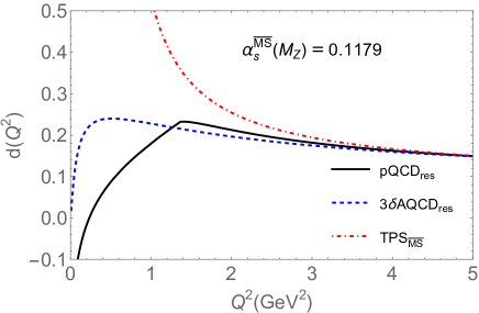
Figure 1: The resummed canonical part of BSR, $d(Q^{2})_{\rm res}$, according to Eq. (30), in the ’P44’ renormalisation scheme with $c_{2}=9.$ and $c_{3}=20.$, for $N_{f}=3$ (’${\rm pQCD}_{\rm res}$’). The strength of the coupling is determined by the choice $\alpha_{s}(M_{Z}^{2};\overline{\rm MS})=0.1179$. The resummation with the corresponding 3$\delta$AQCD coupling is included, for comparison (’${\rm 3dAQCD}_{\rm res}$’). Further, we include the evaluation as the truncated perturbation series (TPS) in powers of $a=a(Q^{2})$ in $\overline{\rm MS}$ scheme, up to $\sim a^{5}$ term and with the central value Eq. (5) of the corresponding coefficient, $d_{4}^{\overline{\rm MS}}=1557.4$ (’${\rm TPS}_{\overline{\rm MS}}$’).

We can see in this Figure that the curve loses its expected monotonically decreasing behaviour for $Q^{2}<1.44\ {\rm GeV}^{2}$. This occurs because for such low $Q^{2}$ the effects of the Landau singularities of the pQCD running coupling $a(te^{-{\widetilde{K}}}Q^{2}+i\epsilon)$ in the integral (30) become significant. Stated otherwise, the used renormalon-motivated resummation in the considered scheme starts failing at $Q^{2}<1.44\ {\rm GeV}^{2}$ due to (unphysical) Landau singularities of the pQCD running coupling. In Fig. 1 we included, for comparison, the results of resummation Eq. (31) when the coupling $a(Q^{2})\mapsto\mathcal{A}(Q^{2})$ is holomorphic (i.e., without Landau singularities). We used a specific 3$\delta$AQCD coupling in miniMOM scheme, for the case $\alpha_{s}(M_{Z}^{2};\overline{\rm MS})=0.1179$ and with the spectral function ${\rho}(\sigma)\equiv{\rm Im}\mathcal{A}(-\sigma-i\epsilon)$ with the threshold value $\sigma_{\rm thr}=M_{1}^{2}=0.150^{2}\ {\rm GeV}^{2}$, for details see 3dAQCD .

VI Fitting to the experimental data and conclusions

In Figs. 2 we present the numerical results for the inelastic BSR ${\overline{\Gamma}}_{1}^{p-n}(Q^{2})$ from various experiments, with the statistical and systematic uncertainties .

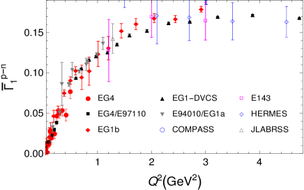
Figure 2: The measured results for the inelastic BSR ${\overline{\Gamma}}_{1}^{p-n}(Q^{2})$ for different experiments, with the statistical (left Figure) and systematic (right Figure) uncertainties.

We will perform the fit by using for $d(Q^{2})$ the resummed expression (30) with the ($N_{f}=3$) pQCD coupling in the P44-renormalisation scheme with $c_{2}=9.$ and $c_{3}=20.$, such that it corresponds to $\alpha_{s}(M_{Z}^{2};\overline{\rm MS})=0.1179$ ($N_{f}=5$) which is the central value of the world average PDG2023 . The number of fit parameters will be either ${\bar{f}}_{2}$ or (${\bar{f}}_{2}$, $\mu_{6}$), i.e., we truncate the OPE (2) at $D=2$ ($i=2$) or $D=4$ ($i=3$). We do not know which experimental uncertainties are correlated and which are not. The statistical uncertainties could be considered to be uncorrelated, but the correlations of the systematic uncertainties are expected to be considerable and difficult to estimate. Therefore, we follow the method of unbiased estimate Deuretal2022 ; PDG2020 ; Schmell1995 : a fraction of systematic uncertainty is added in quadrature to the statistical uncertainty, $\sigma^{2}(Q_{j}^{2})=\sigma^{2}_{\rm stat}(Q_{j}^{2})+k\sigma^{2}_{\rm sys}(Q_{j}^{2})$, we consider then these $\sigma(Q_{j}^{2})$ as uncorrelated, and we determine the fit parameters (${\bar{f}}_{2}$; or ${\bar{f}}_{2}$ and $\mu_{6}$) by minimising the corresponding $\chi^{2}/{\rm n.d.f.}$ for points in a chosen fixed interval $[Q^{2}_{\rm min},Q^{2}_{\rm max}]$ (with $Q^{2}_{\rm max}=4.74\ {\rm GeV}^{2}$). We continue adjusting the fraction parameter $k$ and minimising again, iteratively, until we obtain, when minimising, $\chi^{2}/{\rm n.d.f.}=1$. In practice, we always obtain $0<k<0.5$. The experimental uncorrelated uncertainty (exp.u.) of the extracted parameters is then obtained by the conventional methods (cf. App. of Ref. Bo2011 , App. D of ACT2023 ). The correlated experimental uncertainties (exp.c.) are then obtained by shifting the central experimental values ${\overline{\Gamma}}_{1}^{p-n}(Q^{2}_{j})$ by $(1-\sqrt{k})\sigma_{\rm sys}(Q_{j}^{2})$ up and down and reperforming the fit for these values.

We point out that the smaller the obtained value of $k$, the better the fit. It turns out that, in the above approach, the results depend considerably on the value of $Q^{2}_{\rm min}$ that we choose. We chose $Q^{2}_{\rm min}=1.71\ {\rm GeV}^{2}$ for the fit with two parameters (${\bar{f}}_{2}$, $\mu_{6}$) for the following reasons. 1.) If we decrease $Q^{2}_{\rm min}$ to the adjacent lower neighbouring data points, the value of $k$ increases: from $k=0.162$ (for $Q^{2}_{\rm min}=1.71\ {\rm GeV}^{2}$) to $k=0.172,0.201$ (for $Q^{2}_{\rm min}=1.59,1.50\ {\rm GeV}^{2}$). If we decrease $Q^{2}_{\rm min}$ one step further, to $1.44\ {\rm GeV}^{2}$, then we can see numerically that the evaluation of $d(Q^{2})$ via Eq. (30) is already on the border of applicability at such $Q^{2}$, due to the effects of the Landau singularities of $a(te^{-{\widetilde{K}}}Q^{2}+i\epsilon)$ in the integral, cf. Fig. 1. On the other hand, increasing $Q^{2}_{\rm min}$ above $1.71\ {\rm GeV}^{2}$ to the upper neighbour $1.915\ {\rm GeV}^{2}$, the value of $k$ increases (to $k=0.180$). If we increase $Q^{2}_{\rm min}$ even further, we obtain the results with strong cancellations between the $D=2$ and $D=4$ terms. For all these reasons, we choose $Q^{2}_{\rm min}=1.71^{+0.205}_{-0.27}\ {\rm GeV}^{2}$, and the value of $k$ parameter is $k=0.1621$.

If the fit is performed only with one fit parameter (${\bar{f}}_{2}$), similar verifications give us $Q^{2}_{\rm min}=1.71^{+0.39}_{-0.27}\ {\rm GeV}^{2}$, and the value of $k$ parameter is $k=0.1487$.

With the approach described above, we obtain the final result for the fits. For the two-parameter fit the result is $k=0.1621$ and

$${\bar{f}}_{2} = -0.160^{-0.007}_{+0.025}(c_{2})^{+0.054}_{-0.039}(c_{3})^{+0.044}_{-0.041}(\alpha_{s})^{-0.012}_{+0.016}(d_{4})\mp 0.043({\rm ren})$$ (37a)

$${}^{+0.016}_{+0.119}(Q^{2}_{\rm min})\pm 0.160({\rm exp.u.})\pm 0.297({\rm exp.c.}),$$

$$\mu_{6} = +0.022^{+0.003}_{-0.008}(c_{2})^{-0.013}_{+0.004}(c_{3})^{-0.010}_{+0.008}(\alpha_{s})^{+0.002}_{-0.003}(d_{4})\mp 0.010({\rm ren})$$ (37b)

$${}^{-0.006}_{-0.053}(Q^{2}_{\rm min})\pm 0.062({\rm exp.u.})\mp 0.059({\rm exp.c.})\;[GeV^{4}].$$

The quantity $\mu_{6}$ is in units of ${\rm GeV}^{4}$. Here, the uncertainties at ’$(c_{2})$’ and ’$(c_{3})$’ come from renormalisation scheme variation Eq. (36). The uncertainty at ’$(\alpha_{s})$’ comes from the world average uncertainty $\alpha_{s}(M_{Z}^{2};\overline{\rm MS})=0.1179\pm 0.0009$ PDG2023 . The uncertainty at ’$(d_{4})$’ comes from the variation of $d_{4}$ in such a way that the corresponding (5-loop) $\overline{\rm MS}$ value $d_{4}^{\overline{\rm MS}}$ varies according to Eq. (5). The uncertainty at ’(ren)’ is the renormalon uncertainty, it comes when in the evaluation of $d(Q^{2})$, Eq. (30), we add or subtract the same integral, but imaginary part (divided by $\pi$) instead of the real part [$\pm(1/\pi){\rm Im}(\ldots)$]. These are all the theoretical uncertainties.

The uncertainty at ’($Q^{2}_{\rm min}$)’ can be regarded as coming primarily from experimental uncertainties, and it originates from the variation $Q^{2}_{\rm min}=1.71^{+0.205}_{-0.27}\ {\rm GeV}^{2}$ as mentioned above. The experimental uncertainties at ’(exp.u.)’ and ’(exp.c.)’ were discussed in the previous paragraphs.

The one-parameter fit (${\bar{f}}_{2}$) gives, on the other hand, $k=0.1487$ and

$${\bar{f}}_{2} = -0.107^{-0.001}_{+0.007}(c_{2})^{+0.022}_{-0.029}(c_{3})\pm 0.020(\alpha_{s})\mp 0.009(d_{4})\mp 0.067({\rm ren})$$ (38)

$${}^{+0.012}_{-0.029}(Q^{2}_{\rm min})\pm 0.033({\rm exp.u.})\pm 0.154({\rm exp.c.}),$$

Here, the uncertainty ($Q^{2}_{\rm min}$) comes from $Q^{2}_{\rm min}=1.71^{+0.39}_{-0.27}\ {\rm GeV}^{2}$ as mentioned above.

We note that we keep the (central) value of the parameter $k$ fixed under all the variations, except the variations of ($Q^{2}_{\rm min}$) where the amount of included experimental data points is varied and we require again $\chi^{2}/{\rm n.d.f}=1$.

Furthermore, if we did not include the charm decoupling violation terms $\delta d(Q^{2})_{m_{c}}$, Eq. (6), in our analysis, then the results would change marginally: the central values in Eqs. (37) would change from $-0.160$ and $+0.022$ to $-0.165$ and $+0.023$, respectively, and in Eq. (38) the central value would change from $-0.107$ to $-0.108$, and all the uncertainties would remain practically unchanged. The $k$ parameter values would change from $0.1621$ and $0.1487$ to $0.1626$ and $0.1493$, respectively.

The above results show that we have a competition between various theoretical uncertainties (which are in general moderate) and various experimental uncertainties of the extracted values. The latter uncertainties are large and are in general dominant over the theoretical uncertainties. The experimental uncertainties of the extracted parameter values have their origin, directly or indirectly, in the large statistical and systematic uncertainties of the BSR data points.

As mentioned earlier, the large experimental uncertainties of the data points make the deduction of the preferred value of $\alpha_{s}$ from the BSR data practically impossible, especially under the variation of $Q^{2}_{\rm min}$, and hence we used the world average data for $\alpha_{s}$.

In Figs. 3 we present the obtained central fit theoretical curves (when truncation is made at $D=4$ and at $D=2$), i.e., when ${\bar{f}}_{2}$ and $\mu_{6}$ have the central values of Eqs. (37) and (38), respectively.

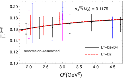
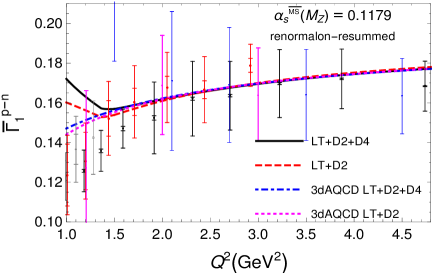
Figure 3: The theoretical OPE curves, when $D=2$ and $D=4$ terms are included, and when only $D=2$ term is included. The results are for the central values of ${\bar{f}}_{2}$ and $\mu_{6}$ obtained from the fit in the interval $Q^{2}_{\rm min}=1.71\ {\rm GeV}^{2}$, Eqs. (37) and (38). The central renormalisation scheme is used (P44 with $c_{2}=9.$ and $c_{3}=20.$). The experimental data are included in the Figures. The left-hand Figure is for $Q^{2}>1.71\ {\rm GeV}^{2}$ (the interval of fitting), and the right-hand Figure has extrapolation to the interval $Q^{2}>1.0\ {\rm GeV}^{2}$. The right-hand Figure contains also the corresponding 3$\delta$AQCD curves, cf. the text for explanations.

For comparison, we included in Figs. 3 the 3dAQCD curves (as in Fig. 1), where the fit for (${\bar{f}}_{2},\mu_{6}$) or (${\bar{f}}_{2}$) was performed, as in pQCD case, for the interval with $Q^{2}_{\rm min}=1.71\ {\rm GeV}^{2}$, and the same values of the $k$ parameter were used as in the pQCD case.

We can also apply, to the same interval of the data points, and for the same values of the $k$ parameter, the two-parameter and one-parameter fit when the canonical BRS part $d(Q^{2})$ is evaluated as a simple truncated perturbation series (TPS), in $\overline{\rm MS}$ scheme and for $\alpha_{s}(M_{Z}^{2};\overline{\rm MS})=0.1179$. We have here additional theoretical uncertainties: the renormalisation scale dependence, and the truncation index ($N_{\rm tr}$) dependence. We choose for simplicity for the renormalisation scale only the value $\mu^{2}=Q^{2}$. Then we obtain for the two-parameter fit (${\bar{f}}_{2}$, $\mu_{6}$) with TPS a strong $N_{\rm tr}$ dependence; at $N_{\rm tr}=8$ we obtain small $\chi^{2}/{\rm n.d.f.}=0.891$, but there ${\bar{f}}_{2}\approx-0.44$ and $\mu_{6}=0.43\ {\rm GeV}^{4}$ are both large and give significant cancellation effects between $D=2$ and $D=4$ BSR terms in the range $2\ {\rm GeV}^{2}<Q^{2}<3\ {\rm GeV}^{2}$. For $N_{\rm tr}\geq 10$ we get $\chi^{2}/{\rm n.d.f.}>4.$, i.e., very large. For the one-parameter fit (${\bar{f}}_{2}$) we obtain for all $N_{\rm tr}\geq 3$ the values $\chi^{2}/{\rm n.d.f.}>1$, and these values increase when $N_{\rm tr}$ increases.

For these reasons, we consider that our renormalon-motivated approach with the resummation Eq. (30) is more reliable than the simpler TPS approach. As a consequence, Eqs. (37) and (38), as well as Figs. 3, represent the central results of our work. Furthermore, the presented work is an example of practical use of known renormalon information for an efficient evaluation (resummation) of the perturbation series of a spacelike observable in pQCD.

In this work, we did not consider models of BSR at very low $Q^{2}\ll 1\ {\rm GeV}^{2}$, such as expansions JeffL2 motivated on chiral perturbation theory or light-front holographic QCD (LFH) model LFH ; LFHBSR . We refer, for example, to ACKS where such models of low-$Q^{2}$ BSR were included in the analyses there. Our analysis here was concentrated on (p)QCD approaches with the use of the QCD running coupling and OPE, and such methods fail are very low values of $Q^{2}$.

The mathematica programs that were constructed and used in the calculations of this work, with the experimental data included, are available on the web page www .

References

• (1) J. D. Bjorken, Phys. Rev. 148 (1966), 1467-1478.
• (2) B. Adeva et al. [Spin Muon (SMC)], Phys. Lett. B 412 (1997), 414-424; D. Adams et al. [Spin Muon (SMC)], Phys. Rev. D 56 (1997), 5330-5358; E. S. Ageev et al. [COMPASS], Phys. Lett. B 612 (2005), 154-164; V. Y. Alexakhin et al. [COMPASS], Phys. Lett. B 647 (2007), 8-17; M. G. Alekseev et al. [COMPASS], Phys. Lett. B 690 (2010), 466-472; C. Adolph et al. [COMPASS], Phys. Lett. B 753 (2016), 18-28; C. Adolph et al. [COMPASS], Phys. Lett. B 769 (2017), 34-41; M. Aghasyan et al. [COMPASS], Phys. Lett. B 781 (2018), 464-472.
• (3) K. Ackerstaff et al. [HERMES], Phys. Lett. B 404 (1997), 383-389; A. Airapetian et al. [HERMES], Phys. Lett. B 442 (1998), 484-492; Phys. Rev. D 75 (2007), 012007.
• (4) K. Abe et al. [E143], Phys. Rev. D 58 (1998), 112003; P. L. Anthony et al. [E142], Phys. Rev. D 54 (1996), 6620-6650; K. Abe et al. [E154], Phys. Rev. Lett. 79 (1997), 26-30; P. L. Anthony et al. [E155], Phys. Lett. B 463 (1999), 339-345; P. L. Anthony et al. [E155], Phys. Lett. B 493 (2000), 19-28.
• (5) A. Deur et al., Phys. Rev. Lett. 93 (2004), 212001.
• (6) A. Deur et al., Phys. Rev. D 78 (2008), 032001.
• (7) K. Slifer et al. [Resonance Spin Structure], Phys. Rev. Lett. 105 (2010), 101601.
• (8) A. Deur et al., Phys. Rev. D 90 (2014) no.1, 012009.
• (9) K. P. Adhikari et al. [CLAS], Phys. Rev. Lett. 120 (2018) no.6, 062501; X. Zheng et al. [CLAS], Nature Phys. 17 (2021) no.6, 736-741; V. Sulkosky et al. [Jefferson Lab E97-110], Phys. Lett. B 805 (2020), 135428.
• (10) C. Ayala, G. Cvetič, A. V. Kotikov and B. G. Shaikhatdenov, Eur. Phys. J. C 78 (2018) no.12, 1002.
• (11) Q. Yu, X. G. Wu, H. Zhou and X. D. Huang, Eur. Phys. J. C 81 (2021) no.8, 690.
• (12) I. R. Gabdrakhmanov, N. A. Gramotkov, A. V. Kotikov, D. A. Volkova and I. A. Zemlyakov, [arXiv:2307.16225 [hep-ph]]; A. V. Kotikov and I. A. Zemlyakov, Phys. Rev. D 107 (2023) no.9, 094034.
• (13) S. J. Brodsky, G. F. de Teramond and A. Deur, Phys. Rev. D 81 (2010), 096010.
• (14) A. Deur, J. M. Shen, X. G. Wu, S. J. Brodsky and G. F. de Teramond, Phys. Lett. B 773, 98 (2017).
• (15) G. Cvetič, Phys. Rev. D 99 (2019) no.1, 014028.
• (16) J. D. Bjorken, Phys. Rev. D 1 (1970), 1376-1379.
• (17) P. A. Zyla et al. [Particle Data Group], PTEP 2020 (2020) no.8, 083C01.
• (18) S. G. Gorishnii and S. A. Larin, Phys. Lett. B 172 (1986), 109-112.
• (19) S. A. Larin and J. A. M. Vermaseren, Phys. Lett. B 259 (1991), 345-352.
• (20) P. A. Baikov, K. G. Chetyrkin and J. H. Kühn, Phys. Rev. Lett. 104 (2010), 132004.
• (21) H. Kawamura, T. Uematsu, J. Kodaira and Y. Yasui, Mod. Phys. Lett. A 12 (1997), 135-143.
• (22) A. L. Kataev and V. V. Starshenko, Mod. Phys. Lett. A 10 (1995), 235-250.
• (23) J. Blümlein, G. Falcioni and A. De Freitas, Nucl. Phys. B 910 (2016) 568.
• (24) R. L. Workman et al. [Particle Data Group], PTEP 2022 (2022), 083C01, and 2023 update.
• (25) D. J. Broadhurst and A. L. Kataev, Phys. Lett. B 315 (1993), 179-187.
• (26) M. Beneke, Phys. Rept. 317 (1999), 1-142.
• (27) A. L. Kataev, JETP Lett. 81 (2005), 608-611.
• (28) A. L. Kataev, Mod. Phys. Lett. A 20 (2005), 2007-2022.
• (29) C. Ayala, G. Cvetič and D. Teca, J. Phys. G 50 (2023) no.4, 045004.
• (30) C. Ayala, G. Cvetič, R. Kögerler and I. Kondrashuk, J. Phys. G 45 (2018) no.3, 035001.
• (31) F. Campanario and A. Pineda, Phys. Rev. D 72 (2005), 056008; C. Ayala and A. Pineda, Phys. Rev. D 106 (2022) no.5, 056023.
• (32) G. Cvetič and I. Kondrashuk, JHEP 12 (2011), 019.
• (33) A. Deur, J. P. Chen, et al. Phys. Lett. B 825 (2022), 136878.
• (34) M. Schmelling, Phys. Scripta 51 (1995), 676-679.
• (35) D. Boito, O. Cata, M. Golterman, M. Jamin, K. Maltman, J. Osborne and S. Peris, Phys. Rev. D 84 (2011), 113006.
• (36) Web page http://www.gcvetic.usm.cl/. The set of mathematica programs is contained in the tarred file fitBSRgenP44res.tar. Some of these programs are interdependent because some of them call some of the others. The central program is fitBSRgenP44res.m.