Extracting Relational Triples Based on Graph Recursive Neural Network via Dynamic Feedback Forest Algorithm

Abstract

Extracting relational triples (subject, predicate, object) from text enables the transformation of unstructured text data into structured knowledge. The named entity recognition (NER) and the relation extraction (RE) are two foundational subtasks in this knowledge generation pipeline. The integration of subtasks poses a considerable challenge due to their disparate nature. This paper presents a novel approach that converts the triple extraction task into a graph labeling problem, capitalizing on the structural information of dependency parsing and graph recursive neural networks (GRNNs). To integrate subtasks, this paper proposes a dynamic feedback forest algorithm that connects the representations of subtasks by inference operations during model training. Experimental results demonstrate the effectiveness of the proposed method.

Introduction

Extracting triples from unstructured documents is a fundamental technology in constructing knowledge bases. This process involves identifying and extracting (subject, predicate, object) from textual input, as depicted in Figure 1. Named entity recognition (NER) and relation extraction (RE) methods can collaborate in the triple extraction pipeline to identify entities and relations, respectively.

Figure 1: An example to extracting the triples from unstructured text

Prior works mainly train these two subtasks separately because there is a cascade process between them, and the output of the NER and the input of the RE subtask are completely different. Despite the flexibility of the pipeline methods, they block the connection between two subtasks. Some approaches [Miwa and Bansal (2016)] overcome the joint extraction problem by sharing features of two subtasks, but two-stage models require separate model training and it is difficult to fully exploit the relationship between subtasks. Despite task conversion resolving this issue by eliminating the cascade process, i.e., converting joint extraction into the sequence labeling process Zheng et al. (2017), their performance is potentially limited by the design of the new tag scheme. Ideally, we hope to overcome these two problems, by integrating two subtasks in one model and not modifying the original tag scheme.

Smoothly integrating cascaded tasks is a nontrivial task. The difficulty lies in that the relation classification (RC) aims to classify the relation between an entity pair while we have not known where are the entities. The main gap between NER and RC subtasks is how to generate relation candidates, which makes model integration a challenging issue. This paper introduces a dynamic feedback forest algorithm (DFF) to integrate subtasks into a joint optimization process by using inference operations during model training. These operations can directly connect the representations of NER and RE. Then, the model can use the original tag to supervise the two subtasks together. The DFF algorithm dynamically constructs multiple subgraphs to form the forest and teach the model according to the deviation of current prediction and ground truth. This algorithm executes the inference and feedback operations during model training, adapting the model to new samples.

The second challenge is to unify the representations of entity and relation. This paper maps the entity and its relation to the dependency graph. We applied the idea of the recursive neural network to the dependency graph so that we could directly label a vertex as an entity, a relation instance, or none. Sometimes, there are different relations between the same entity pair, i.e., “Iraq’s capital is Baghdad” and “Iraq contains Baghdad”, as shown in Figure 1. The prior new tag scheme is incapable of dealing with overlapping relations (an entity belongs to more than one relation). Other works [Wang et al. (2018); Zeng et al. (2018)] design new strategies to solve this problem. Our GRNN model is naturally compatible with different relations between an entity pair without changing the network. To further simplify the network, we also test the hypothesis that a unified representation can be obtained to resolve two subtasks by our GRNN.

We conduct experiments on the NYT dataset. Experimental results demonstrate the effectiveness of our approach. The major contributions of this paper can be summarized below.

(i) This paper explores a graph labeling approach to resolving the triple extraction task.

(ii) This paper utilizes graph recursive networks to model the triple extraction task with joint task learning and joint representation learning.

(iii) This paper introduces the DFF algorithm, which enables the model to connect representations of different subtasks through inference operations during training, facilitating the learning process.

Related Work

For the joint extraction task, Miwa and Bansal (2016) propose a method using sequential and separate tree-structured LSTM-RNNs for NER and RC. Their work represents the relation by the shortest dependency path, while our model uses a vertex to represent any entity or relation. Their method use scheduled sampling, entity pretraining, and label embedding to enhance the training process, while we use the maximum log-likelihood with the DFF algorithm.

Ren et al. (2017) use a domain-agnostic segmentation algorithm to mine entity mentions, and convert the task into a global embedding problem. Khashabi (2013) present a recursive neural network-based method to extract entity and relation separately, but leave the joint learning for future work. Our model solves the joint learning problem.

Zheng et al. (2017) propose a novel tag scheme to convert this task into a sequence labeling problem, but it increases about eight times of classes and cannot deal with the overlapping relations. Wang et al. (2018) propose a neural transition-based approach and a suite of transition schemes, while our method is only based on the graph structure of dependency parsing. Zeng et al. (2018) propose the One-Decoder and Multi-Decoder approaches to extract relational facts with copy mechanism. They divide the sentences into three types according to the triplet overlap degree, and our approach is also compatible with overlapping relations. Liu et al. (2018) propose the Seq2RDF which aims to map textual input to existing RDF triples, so it relies on the knowledge graph vocabulary, while our approach aims to extract triples directly from unstructured documents in a general way.

Methods

Task Definition

Given a text sequence $x=[w_{1},...,w_{n}]$ where $w_{i}$ is the $i$-th token, the triple extraction task aims to extract multiple ($s_{[type]}$, $p$, $o_{[type]}$) where $s$ and $o$ represent two non-overlapping consecutive spans, $s=[w_{s1},w_{s1+1}...,w_{s2}]$ and $o=[w_{o1},w_{o1+1}...,w_{o2}]$. $p\in R$ is the relation type, where $R$ is a set of predefined relation types. The subscript ${}_{[type]}\in C$ is the entity type, where $C$ is a set of predefined entity types.

The Graph Labeling Scheme

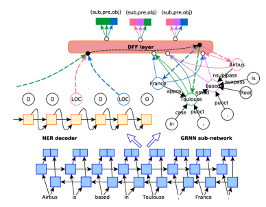
Figure 2: Joint task learning (JTL) network for integrating subtasks

Figure 2 uses an example to demonstrate the idea of how to convert the joint extraction task into a graph labeling problem. The lower layer uses a Bi-LSTM encoder to generate the contextual representation. Then, the intermediate layer uses the Stanford CoreNLP [Manning et al. (2014)] to convert the sentences into dependency graphs. This model uses vertices to represent entities and relations. Finally, this model integrates the subtasks using the DFF algorithm (introduced in subsection Training Algorithm).

We take a simple example to demonstrate the graph labeling scheme. Figure 3 contains three entities (Airbus [ORG], Toulouse [LOC], and France [LOC]). Each entity is mapped to the corresponding vertex. Each relation is mapped to the least common ancestor (LCA) of two entity subgraphs, i.e. the relation of (Airbus, relation, Toulouse) is represented by the vertex “based” which is the LCA of “Airbus” and “Toulouse”, which implies the relation type is “/business/company/place_founded ”.

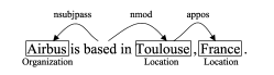
Figure 3: An example to demonstrate the entity and relation representation

Any relation or entity can be represented by a vertex, so this model can directly classify the vertices. For the entity phrase, this model maps each entity as a subgraph and takes the root vertex as the representation like [Khashabi (2013)]. In some cases, two entities share the same root, for example, the Los Angeles Lakers and Kobe Bryant of Figure 4 share the same root Bryant in the dependency graph. To better differentiate the entities, an entity vector is finally composed of the vertex representation and the average pooling of the entity phrase.

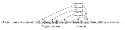
Figure 4: An example that two entities share the same root

Sometimes, there are different relations between two entities. In addition to the 1-of-n classification, this model can be extended to the multi-label classification form which can extract different relations of the same entity pair by multi-label graph labeling for each vertex.

GRNN Units

We have obtained the graph structure of each sample. The gated units and CNN have achieved impressive performances in many deep-learning models. To better process the graph data, we implement different neural units (LSTM [Hochreiter and Schmidhuber (1997)], GRU [Chung et al. (2014)] and CNN [LeCun et al. (1998)]) that are compatible with our GRNN model.

Graph RNN For the basic perceptron, each source vertex accumulates the information from its target vertices through a non-linear activation function as below.

$$h_{t}=tanh(Wx_{t}+\Sigma_{j=0}^{P(t)}U_{m(t,j)}h_{j}+b)$$ (1)

where $W\in\mathbb{R}^{d\times l},U\in\mathbb{R}^{m\times d\times d},h\in\mathbb{R}^{d},x\in\mathbb{R}^{l},b\in\mathbb{R}^{d}$. The $t$ and $j$ are the indexes of the source and target vertices respectively. $P(t)$ is the number of target vertices of the source vertex $t$. $U$ is a group of edge parameters where $m$ denotes the 193 edge types, and $d\times d$ is the dimension of an edge embedding. $U_{m(t,j)}$ denotes the edge embedding that connects source $t$ and target $j$. Considering edge types can make the model control substreams in different weights. $h$ and $x$ denote the vertex representation and input respectively. To resolve the gradient vanishing problem, we also implemented the gated units.

Graph LSTM For the LSTM unit, this paper simplifies the network by using a group of edge parameters (same as the variable $U$ in formulation (1)) based on the study of [Peng et al. (2017)]. Compared with the linear chain LSTM unit, the main improvement is the separate forget gate for each input edge, which can achieve selective control of different edges.

$$i_{t} =\sigma(W_{i}x_{t}+\Sigma_{j=1}^{P(t)}U_{m(t,j)}h_{j}+b_{i})$$ (2)

$$f_{m(t,j)} =\sigma(W_{f}x_{t}+U_{m(t,j)}h_{j}+b_{f})$$ (3)

$$o_{t} =\sigma(W_{o}x_{t}+\Sigma_{j=1}^{P(t)}U_{m(t,j)}h_{j}+b_{o})$$ (4)

$$\tilde{c_{t}} =\tanh(W_{c}x_{t}+\Sigma_{j=1}^{P(t)}U_{m(t,j)}h_{j}+b_{c})$$ (5)

$$c_{t} =i_{t}\odot\tilde{c_{t}}+\Sigma_{j=1}^{P(t)}f_{m(t,j)}\odot c_{j}$$ (6)

$$h_{t} =o_{t}\odot\tanh(c_{t})$$ (7)

where $h$, $c$, and $o$ are the hidden state, the cell state, and the output respectively. $W$, $U$ and $b$ are model parameters. The $\odot$ represents the Hadamard product (pointwise multiplication).

Graph GRU Analogy with the graph LSTM unit, the graph GRU unit separates the reset gate for each edge. In the graph LSTM, the output gate, and the cell state can limit the hidden state into an effective range as formulation (7). However, for the large values of hidden states, the outputs of graph GRU might grow large in magnitude. To counteract this effect, this paper adds a non-linear activation in the edge to limit the response in practice.

$$p_{j} =\tanh(U_{m(t,j)}h_{j})$$ (8)

$$z_{t} =\sigma(W_{z}x_{t}+\Sigma_{j=1}^{P(t)}p_{j}+b_{z})$$ (9)

$$r_{m(t,j)} =\sigma(W_{r}x_{t}+b_{r}+p_{j})$$ (10)

$$\tilde{h_{t}} =\sigma(W_{h}x_{t}+U_{r}\Sigma_{j=1}^{P(t)}(r_{m(t,j)}\odot p_{j})+b_{h})$$ (11)

$$h_{t} =(1-z_{t})\odot\Sigma_{j=1}^{P(t)}p_{j}+z_{t}\tilde{h_{t}}$$ (12)

where $h$, $z$, and $r$ are the output vector, update gate vector and reset gate vector. $W$, $U$ and $b$ are model parameters.

Graph RCNN The recursive neural network [Socher et al. (2013)] can only process the binary combination and is not suitable for graph data, since a source vertex may have two or more targets. This paper adopts the RCNN unit [Zhu et al. (2015)] which can deal with the k-ary parsing tree. To make the RCNN unit compatible with our GRNN, we add different edge types and generalize the RCNN unit to DAG.

Convolutional neural networks [LeCun et al. (1998)] utilize layers with convolving filters to extract local features. CNN models have been proven effective for many NLP tasks [Collobert et al. (2011)].

$$H^{(t)}=tanh(W*X)$$ (13)

where $*$ denotes the 1-D convolution. $W\in\mathbb{R}^{c\times l}$ is the convolving filter where $c$ is window size and $l$ is vector dimension. As shown in Figure 5, the left part is the predicted triples and the right part is a graph RCNN network. The input $X\in\mathbb{R}^{P(t)\times l}$ is composed of $v_{(t,i)}$. Let $\oplus$ represent the concatenation operation.

$$X =[v_{(t,1)},v_{(t,2)}...,v_{(t,P(t)}]$$ (14)

$$v_{(t,i)} =x_{t}\oplus h_{t(i)}\oplus d_{(t,i)}$$ (15)

where the $x_{t}$ is the word embedding of the current (source) vertex. The $h_{t(i)}$ $(i=1,...P(t))$ denotes the representation of the $i$-th target vertex of source vertex $t$. $d_{(t,i)}$ is the distance embedding [Zhu et al. (2015)] of vertex $i$. The distance embedding is a way to represent the relative distance between the source vertex $t$ and the $i$-th target vertex with a fixed length vector. To keep the order invariant, for the target vertices, this network uses the natural order of words in the sentence. The vertex without any target vertex consists of its word embedding and a zero vector. The output of the convolution operation is $H^{(t)}=[h_{1},h_{2},...,h_{K}]$ where $K$ is dynamic depending on the number of target vertices. Then the pooling operation captures the most informative features on rows.

$$h_{t}=\max\limits_{j}H_{ij}^{(t)}$$ (16)

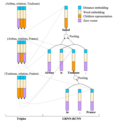
Figure 5: The GRNN-RCNN extraction example of ”Airbus is based in Toulouse, France.”

The above neural units enhance the graph data processing through different feature extraction operations. To reduce the computational complexity, we set the maximum recursive depth to 6. The uni-directional GRNN is a top-down process, and we also built the bidirectional GRNN which can capture the features of both top-down and bottom-up directions.

Joint Learning Networks

We employ two networks to integrate our neural units. The main difference between the two networks is the way they decode each subtask.

Joint task learning network. As shown in Figure 2, the higher layer uses two decoders to jointly learn task-specific representations. We refer to it as joint task learning (JTL).

For the NER subtask, we adopt the BIOES scheme [Ratinov and Roth (2009)] in a uni-directional LSTM-RNN. To keep more influence of the previous step this decoder also inputs the previous hidden state to the current step. For the RE subtask, the input of GRNN is a graph where each vertex is mapped to the contextual representation of the encoder layer. The edge embeddings are jointly learned to control children’s streams. The vertices of GRNN are mainly used to construct triple representations for the RC subtask.

Joint representation learning network. To test whether this network can learn a unified representation [Zhu (2023a, 2022a)], we simplify the network by only keeping the standalone decoder. We refer to it as the joint representation learning (JRL) network, as shown in Figure 6. The output of the encoder layer is input to the GRNN sub-network, and then the two subtasks directly use the representation of these vertices for prediction.

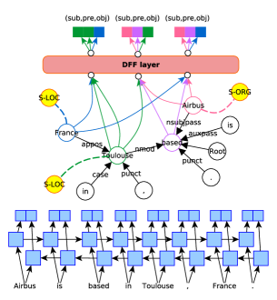
Figure 6: JRL network for integrating subtasks and representations

Training Algorithm

During model training, the DFF algorithm has an inference operation that predicts entities and dynamically generates triple candidates using all possible combinations of entities. This algorithm enables the model to dynamically adapt to new patterns in the data. The downside is that there is a sort of information loss [Zhu et al. (2022)] in the discrete inference process.

This algorithm mainly contains two steps, inference, and feedback, as shown in algorithm 1.

(1) In the inference step, this model first predicts/infers the label sequence, as shown in line 1, and uses the combination of the predicted entities as triple candidates, as shown in lines 2-3. Then, the model dynamically extracts subgraphs of multiple triples to construct the forest on the top layer, as shown in lines 5-9. This model uses the indices of $s$ and $o$ to find the LCA index as $p_{w}$. Then, the model will map the above indices into the GRNN to get the vector representations for a triple as shown in line 8. In lines 10-16, this model also memorizes the unexpected entity pairs that are not predicted, using the same operations of lines 5-9.

(2) In the feedback step, this model generates the relation type assumption for each predicted triple by using a single-layer neural network, as shown in line 17. Then, it compares the assumptions with the ground truth to get the feedback signal to update the model state through backpropagation. The feedback signal is generated by the loss function to calculate the gradients, as shown below.

$$\max\limits_{\theta}L =\sum\limits_{i=1}^{|\mathbb{D}|}(\log\prod\limits_{j}p_{ner}(y_{ner_{j}}^{(i)}|{\bf z}_{i};\theta)+\log\prod\limits_{k}p_{re}(y_{re_{k}}^{(i)}|{\bf z}_{i};\theta))$$

where the $p_{ner}$ and $p_{re}$ represent the prediction of the actual class of NER and RE subtasks respectively. $|\mathbb{D}|$ is the dataset size and $z$ denotes the input sequence. $j$ and $k$ denote the indices of the entity or relation respectively. $\theta$ is the model parameter. The final model generated by the DFF algorithm is a recursive computational graph where the parameters can be optimized jointly.

1     Input:NER decoding vectors $v$, NER labels $l_{ner}$, Triples $l_{re}$, vertex vectors $V$

2    Output:The loss values of subtasks

1:  Predict the label sequence $\hat{y}_{ner}$ based on $v$

2:  Extract entity phrases $ens$ from the $\hat{y}_{ner}$

3:  Generate entity $pairs$ using binary combination of $ens$

4:  $\hat{y}_{rc}$=[], $l_{rc}$=[]

5:  for  $j\leftarrow 0,l_{re}.length-1$ do

6:     $s,p,o$=$l_{re}$[$j$]

7:     Find the LCA index for $s$ and $o$ as $p_{w}$

8:     Generate $v_{t}$=[$v_{s}$,$v_{p_{w}}$,$v_{o}$] from $V$ according to indices ($s$,$p_{w}$,$o$), then, add $v_{t}$ to memory $\hat{y}_{rc}$ and add relation $p$ to $l_{rc}$ respectively

9:  end for

10:  for $j\leftarrow 0,pairs.length-1$ do

11:     if $pairs$[$j$] not in $l_{re}$ then

12:        $s,o$=$pairs$[$j$]

13:        Find the LCA index for $s$ and $o$ as $p_{w}$

14:        Generate $v_{t}$=[$v_{s}$,$v_{p_{w}}$,$v_{o}$] from $V$ according to indices ($s$,$p_{w}$,$o$), then, add $v_{t}$ to memory $\hat{y}_{rc}$ and add relation “None” to $l_{rc}$ respectively

15:     end if

16:  end for

17:  $assump$ = predict($\hat{y}_{rc}$)

18:  feedback($\hat{y}_{ner}$, $l_{ner}$), feedback($assump$, $l_{rc}$)

Algorithm 1 The DFF algorithm

Experiments

Experiment Setup

Dataset

The NYT dataset is generated by aligning the Freebase relations with the news article of the 1987 $\sim$ 2007 New York Times. The training set contains 1.18M sentences with 47 entity types and 24 relation types [Ren et al. (2017)], i.e., “/business/company/founders”, “/sports/sports_team/location”, etc. We exclude the “None” label relation, like [Zheng et al. (2017); Ren et al. (2017)]. During the training process, the samples with only the “None” label relations have little effect on the final result and we remove them. Thus, we use 66,336 training samples (about 1/3 of the training set) to reduce the training time. The test set contains 395 samples manually annotated by the author of [Hoffmann et al. (2011)].

Evaluation

We adopt the standard micro F1 score, recall (Rec.), and precision (Prec.) as the metrics for the NER and RE subtasks. For the final result, a correct prediction is that the extracted triple matches the ground truth including two entities, relation direction and relation type. For the NER subtask, we consider the entity type, length, and position in sentences.

Hyperparameters

The input word is projected to a 200-D pre-trained GloVe [Pennington, Socher, and Manning (2014)] word embedding. The hidden state of the encoder is 300-D. The dimension of GRNN units (including the LSTM, GRU and RCNN units) is 100-D. We split the training data into 100 pieces to select better models. We first use the single-sample training to get a good model and then adopt the batch (64) training to fine-tune the model. We ran the experiments on an AMD Ryzen 5 1500X Quad-Core Processor @ 3.5GHz (Mem: 16G) and RTX 1070Ti GPUs (8G).

Results of JTL network

This subsection first reports the results of the 1-of-n classification form. We use Bi to represent the bidirectional modeling. The RCNN, GRU, and LSTM denote the computational units in the GRNN models.

Table 1 reports the results. The first two parts are the pipeline methods and the joint extraction methods respectively. The third part is our methods where different units are implemented to augment the basic GRNN. To eliminate the influence of random factors we ran the experiments three times and take the average.

The basic GRNN (Bi-GRNN) also gets a good result, which means that the mechanism of the GRNN is effective in this task. Compared with other studies, the results of GRNN models are more balanced, while the recall and precision of other joint extraction models are not balanced enough. This indicates that using the global optimization process allows the model to find a better balance. The gated units improve the results since they alleviate the gradient vanishing problem. This indicates considering long-time graph dependency can help to encode rich relation representation.

Table 1: Results report of the joint entity and relation extraction methods on the NYT dataset

Methods	Prec.	Rec.	F1
FCM [Mintz et al. (2009)]	25.8	39.3	31.1
LINE [Tang et al. (2015)]	33.5	32.9	33.2
MultiR [Hoffmann et al. (2011)]	33.8	32.7	33.3
DS-Joint [Li and Ji (2014)]	57.4	25.6	35.4
Linear-Tree [Miwa and Bansal (2016)]	37.3	15.4	23.4
CoType [Ren et al. (2017)]	42.3	51.1	46.3
LSTM-LSTM-Bias [Zheng et al. (2017)]	61.5	41.4	49.5
Transition [Wang et al. (2018)]	64.3	42.1	50.9
Bi-GRNN	51.5	48.8	50.1
GRNN-RCNN	58.3	45.4	51.0
Bi-GRNN-GRU	55.5	48.9	52.0
Bi-GRNN-LSTM	54.9	50.5	52.6

Results of JRL network

To evaluate whether this model can obtain a unified representation, we test the JRL network of Figure 6. We use Standalone to represent the LSTM-based JRL network.

Comparison of JTL and JRL networks

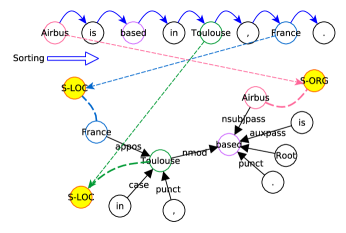
Figure 7: An example of enhancing NER representation in the JRL network by sorting vertices

As shown in table 2, the precision of the Bi-Standalone model is high but the recall decreases since we did not consider the influence of token order. To encode this factor, the Standalone model considers the bigram of vertices, more formally, $h_{t}^{{}^{\prime}}=\mbox{ReLU}(W(h_{t-1}^{{}^{\prime}}\oplus h_{t})+b)$, where $t$ is the time step and $h_{t}$ is the t-th vertex vector. $\oplus$ denotes the concatenation operation. $W$ and $b$ are the linear composition matrix and bias vector respectively. $h_{-1}^{{}^{\prime}}$ is initialized to a zero vector.

This setting improves 4.40% and 2.90% F1 scores on the NER and RE subtasks, respectively. Although such a strategy is naive, by using the $W,b$ parameters, this model achieves a competitive result (52.6% F1 score) to the LSTM decoder. This is because the NER representation is enhanced by the RE subtask by jointly updating the model. This indicates that keeping order invariant is essential.

Table 2: Results report where the first (1-4 rows) and the second (5-8 rows) parts are the results of JTL and JRL networks respectively

Tasks	NER			RE
Methods	Prec.	Rec.	F1	Prec.	Rec.	F1
Bi-GRNN	91.9	90.8	91.3	51.5	48.8	50.1
GRNN-RCNN	92.1	91.4	91.7	58.3	45.4	51.0
Bi-GRNN-GRU	92.5	90.9	91.7	55.5	48.9	52.0
Bi-GRNN-LSTM	92.1	91.5	91.8	54.9	50.5	52.6
Standalone	84.2	79.8	81.9	52.9	41.4	46.4
Bi-Standalone	89.3	85.7	87.4	53.8	45.9	49.6
Standalone+sort	91.2	89.5	90.3	51.2	48.4	49.8
Bi-Standalone+sort	92.1	91.5	91.8	54.5	50.8	52.6

Comparison of the training process

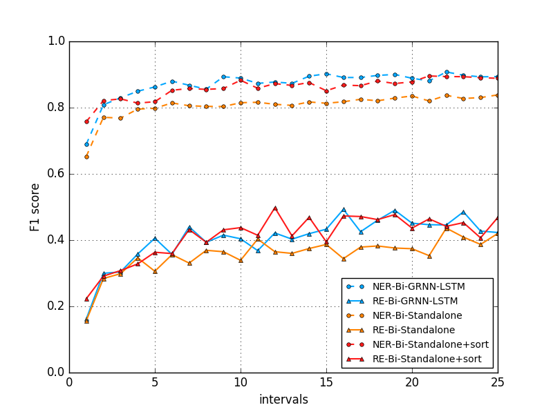
Figure 8: Learning process in the first epoch (average sampling 25 intervals)

To observe the training process, we split the first training epoch into 25 intervals and evaluate the models of table 2 on the test set. As shown in Figure 8, the JTL and JRL networks learn the NER and RE subtasks simultaneously. The learning process is effective, and some model states achieved good results. This suggests that the model selection is important in this approach.

We also observe the Bi-Standalone+sort (sorted JRL as shown in Figure 7) achieved higher results on the RE subtask than the Bi-GRNN-LSTM. This is because the JRL network encodes more entity information in the relation representation. This experiment shows that using the same learning representation for different subtasks can help compress model parameters.

Conclusion

This paper introduces a novel approach to extracting relational triples from English textual input by leveraging graph recursive network models. The proposed methods integrate named entity recognition (NER) and relation extraction (RE) subtasks in a joint optimization process, utilizing the GRNN and the DFF training algorithm. This approach eliminates the need for designing new tag schemes and bridges the gap between subtasks by connecting the representations in both subtasks through inference operations during model training. Experimental results demonstrate the effectiveness of our model in integrating subtasks and representations. Moreover, this model can be adapted to encode subgraphs [Zhu (2022c)] and applied in downstream applications [Zhu (2023b, 2022b)].

References

- Chung et al. (2014) Chung, J.; Gulcehre, C.; Cho, K.; and Bengio, Y. 2014. Empirical evaluation of gated recurrent neural networks on sequence modeling. arXiv preprint arXiv:1412.3555.
- Collobert et al. (2011) Collobert, R.; Weston, J.; Bottou, L.; Karlen, M.; Kavukcuoglu, K.; and Kuksa, P. 2011. Natural language processing (almost) from scratch. Journal of Machine Learning Research 12(Aug):2493–2537.
- Hochreiter and Schmidhuber (1997) Hochreiter, S., and Schmidhuber, J. 1997. Long short-term memory. Neural computation 9(8):1735–1780.
- Hoffmann et al. (2011) Hoffmann, R.; Zhang, C.; Ling, X.; Zettlemoyer, L.; and Weld, D. S. 2011. Knowledge-based weak supervision for information extraction of overlapping relations. In Proceedings of the ACL 2011, 541–550. Association for Computational Linguistics.
- Khashabi (2013) Khashabi, D. 2013. On the recursive neural networks for relation extraction and entity recognition.
- LeCun et al. (1998) LeCun, Y.; Bottou, L.; Bengio, Y.; and Haffner, P. 1998. Gradient-based learning applied to document recognition. Proceedings of the IEEE 86(11):2278–2324.
- Li and Ji (2014) Li, Q., and Ji, H. 2014. Incremental joint extraction of entity mentions and relations. In Proceedings of the ACL 2014, volume 1, 402–412.
- Liu et al. (2018) Liu, Y.; Zhang, T.; Liang, Z.; Ji, H.; and McGuinness, D. L. 2018. Seq2rdf: An end-to-end application for deriving triples from natural language text. arXiv preprint arXiv:1807.01763.
- Manning et al. (2014) Manning, C.; Surdeanu, M.; Bauer, J.; Finkel, J.; Bethard, S.; and McClosky, D. 2014. The stanford corenlp natural language processing toolkit. In Proceedings of ACL 2014, 55–60.
- Mintz et al. (2009) Mintz, M.; Bills, S.; Snow, R.; and Jurafsky, D. 2009. Distant supervision for relation extraction without labeled data. In Proceedings of the ACL 2009, 1003–1011. Association for Computational Linguistics.
- Miwa and Bansal (2016) Miwa, M., and Bansal, M. 2016. End-to-end relation extraction using lstms on sequences and tree structures. arXiv preprint arXiv:1601.00770.
- Peng et al. (2017) Peng, N.; Poon, H.; Quirk, C.; Toutanova, K.; and Yih, W.-t. 2017. Cross-sentence n-ary relation extraction with graph lstms. arXiv preprint arXiv:1708.03743.
- Pennington, Socher, and Manning (2014) Pennington, J.; Socher, R.; and Manning, C. 2014. Glove: Global vectors for word representation. In Proceedings of the EMNLP 2014, 1532–1543.
- Ratinov and Roth (2009) Ratinov, L., and Roth, D. 2009. Design challenges and misconceptions in named entity recognition. In Proceedings of the CoNLL 2009, 147–155. Association for Computational Linguistics.
- Ren et al. (2017) Ren, X.; Wu, Z.; He, W.; Qu, M.; Voss, C. R.; Ji, H.; Abdelzaher, T. F.; and Han, J. 2017. Cotype: Joint extraction of typed entities and relations with knowledge bases. In Proceedings of the WWW 2017, 1015–1024. International World Wide Web Conferences Steering Committee.
- Socher et al. (2013) Socher, R.; Bauer, J.; Manning, C. D.; et al. 2013. Parsing with compositional vector grammars. In Proceedings of the ACL 2013, volume 1, 455–465.
- Tang et al. (2015) Tang, J.; Qu, M.; Wang, M.; Zhang, M.; Yan, J.; and Mei, Q. 2015. Line: Large-scale information network embedding. In Proceedings of the WWW 2015, 1067–1077. International World Wide Web Conferences Steering Committee.
- Wang et al. (2018) Wang, S.; Zhang, Y.; Che, W.; and Liu, T. 2018. Joint extraction of entities and relations based on a novel graph scheme. In IJCAI, 4461–4467.
- Wu et al. (2018) Wu, Z.; Ren, X.; Xu, F. F.; Li, J.; and Han, J. 2018. Indirect supervision for relation extraction using question-answer pairs. In Proceedings of the Eleventh ACM International Conference on Web Search and Data Mining, 646–654. ACM.
- Zeng et al. (2018) Zeng, X.; Zeng, D.; He, S.; Liu, K.; and Zhao, J. 2018. Extracting relational facts by an end-to-end neural model with copy mechanism. In Proceedings of the ACL 2018, volume 1, 506–514.
- Zheng et al. (2017) Zheng, S.; Wang, F.; Bao, H.; Hao, Y.; Zhou, P.; and Xu, B. 2017. Joint extraction of entities and relations based on a novel tagging scheme. arXiv preprint arXiv:1706.05075.
- Zhu et al. (2015) Zhu, C.; Qiu, X.; Chen, X.; and Huang, X. 2015. A re-ranking model for dependency parser with recursive convolutional neural network. arXiv preprint arXiv:1505.05667.
- Zhu et al. (2022) Zhu, H.; Tiwari, P.; Zhang, Y.; Gupta, D.; Alharbi, M.; Nguyen, T. G.; and Dehdashti, S. 2022. Switchnet: A modular neural network for adaptive relation extraction. Computers and Electrical Engineering 104:108445.
- Zhu (2022a) Zhu, H. 2022a. Financial data analysis application via multi-strategy text processing. arXiv preprint arXiv:2204.11394.
- Zhu (2022b) Zhu, H. 2022b. Metaaid: A flexible framework for developing metaverse applications via ai technology and human editing. arXiv preprint arXiv:2204.01614.
- Zhu (2022c) Zhu, H. 2022c. Metaonce: A metaverse framework based on multi-scene relations and entity-relation-event game. arXiv preprint arXiv:2203.10424.
- Zhu (2023a) Zhu, H. 2023a. Fqp 2.0: Industry trend analysis via hierarchical financial data. arXiv preprint arXiv:2303.02707.
- Zhu (2023b) Zhu, H. 2023b. Metaaid 2.0: An extensible framework for developing metaverse applications via human-controllable pre-trained models. arXiv preprint arXiv:2302.13173.