Supersymmetric hybrid inflation and metastable cosmic strings in $SU(4)_{c}\times SU(2)_{L}\times U(1)_{R}$

Abstract

We construct a realistic supersymmetric model for superheavy metastable cosmic strings (CSs) that can be investigated in the current pulsar timing array (PTA) experiments. We consider shifted $\mu$ hybrid inflation in which the symmetry breaking $SU(4)_{c}\times SU(2)_{L}\times U(1)_{R}\rightarrow SU(3)_{c}\times SU(2)_{L}\times U(1)_{B-L}\times U(1)_{R}$ proceeds along an inflationary trajectory such that the topologically unstable primordial monopoles are inflated away. The breaking of $U(1)_{B-L}\times U(1)_{R}\rightarrow U(1)_{Y}$ after inflation ends yields the metastable CSs that generate the stochastic gravitational wave background (SGWB) which is consistent with the current PTA data set. The scalar spectral index $n_{s}$ and the tensor to scalar ratio $r$ are also compatible with Planck 2018. We briefly discuss both reheating and leptogenesis in this model.

I Introduction

The pulsar timing array experiments have recently shared evidence for the presence of a stochastic gravitational background [1, 2, 3, 4, 5], which may be compatible with the emission of such background by superheavy metastable [6, 7, 8, 9, 10, 11] or quasi-stable [12] cosmic strings (CSs). For a recent discussion of composite topological structures in SO(10), more precisely Spin (10), see ref. [13].

In this paper we describe how the desired metastable strings appear in a realistic supersymmetric inflation model based on the gauge symmetry $G=SU(4)_{c}\times SU(2)_{L}\times U(1)_{R}$, a well- known subgroup of $SO(10)$. Supersymmetric hybrid inflation models have been extensively studied in [14, 15, 16, 17, 18, 19, 20, 21, 22, 23, 24, 25, 26, 27, 28] and for tribrid inflation see [29]. Here we utilize one particular version known as $\mu$ - hybrid inflation [30, 31, 32, 33, 34]. Following [35, 13], the breaking of $SU(4)_{c}$ to $SU(3)_{c}\times U(1)_{B-L}$ at a scale close to $M_{GUT}$ produces ‘red’ monopoles, that we show are inflated away by employing shifted $\mu$ - hybrid inflation [36]. The subsequent breaking of $U(1)_{B-L}\times U(1)_{R}$ to $U(1)_{Y}$, also close to $M_{GUT}$, takes place after the inflationary phase is effectively over. This produces the desired metastable strings that generate a stochastic gravitational wave background. The strings eventually disappear from the quantum tunneling of the red monopole-antimonopole pairs.

The paper is laid out as follows. In section II we summarize the salient features of the $SU(4)_{c}\times SU(2)_{L}\times U(1)_{R}$ model including symmetry breaking and evolution of the gauge couplings. The shifted $\mu$-hybrid inflationary scenario is presented in section III, and in section IV we discuss the supergravity corrections with non-minimal Kähler potential. The global minimum and symmetry breaking after inflation is discussed in section V. Section VI summarizes how reheating and leptogenesis proceed in this model, together with the inflationary predictions. The metastable strings and predictions related to gravitational waves (GW) are presented in section section VII. Our conclusions are given in section VIII.

II Supersymmetric $SU(4)_{c}\times SU(2)_{L}\times U(1)_{R}$ Model

Table 1: Matter and Higgs superfields together with their decomposition under $SU(4)_{c}\times SU(2)_{L}\times U(1)_{R}=421$ the $SU(3)_{c}\times SU(2)_{L}\times U(1)_{Y}=$ SM and their $R$ charges.

Superfields	$421$	SM	$q(R)$
$F_{\ i}$	$({4,\ 2,\ 0})$	$Q_{i}(3,\ 2,\ 1/6)$	1/2
		$L_{i}(1,\ 2,\ -1/2)$
$F^{c}_{u\ i}$	$(\overline{4},\ 1,\ -1/2)$	$U^{c}_{i}(\overline{3},\ 1,\ -2/3)$	1/2
		$N^{c}_{i}(1,\ 1,\ 0)$
$F^{c}_{d\ i}$	$(\overline{4},\ 1,\ 1/2)$	$D^{c}_{i}(\overline{3},\ 1,\ 1/3)$	1/2
		$E^{c}_{i}\ (1,\ 1,\ 1)$
$H$	$({4,\ 1,\ 1/2})$	$(3,\ 1,\ 1/6)$	0
		$(1,\ 1,\ \ 0)$
$\overline{H}$	$(\overline{4},\ 1,\ -1/2)$	$(\overline{3},\ 1,\ \ \ -2/3)$	0
		$({1,\ 1},\ \ 0)$
$S$	$({1,\ 1,\ 1})$	$({1,\ 1},\ \ \ 0)$	1
$\Phi$	$({15,\ 1,\ 0})$	$({1,\ 1},\ 0)$	0
		$({8,\ 1},\ \ 0)$
		$({3,\ 1},\ \ \ 1/3)$
		$({\overline{3},\ 1},\ \ -1/3)$
$h_{u}$	$({1,\ 2,\ \ \ 1/2})$	$\ ({1,\ 2},\ \ \ 1/2)$	0
$h_{d}$	$({1,\ 2,\ \ -1/2})$	$\ ({1,\ 2},\ \ \ 1/2)$	0

The superfields containing standard model (SM) matter and Higgs content and their $U(1)_{R}$ charges are given in table 3. The $U(1)_{R}$ symmetric superpotential for shifted $\mu$-hybrid inflation is written as,

$$W =S\left(\kappa M^{2}-\kappa\,\text{Tr}(\Phi^{2})-\dfrac{\beta}{M_{\star}}\,\text{Tr}(\Phi^{3})\right)$$

$$+\lambda_{H}\,S\,H\,\overline{H}+\lambda_{h}\,S\,h_{u}\,h_{d}$$

$$+\lambda^{(u,\nu)}_{ij}F_{i}F^{c}_{u\ j}h_{u}+\lambda^{(d,e)}_{ij}F_{i}F^{c}_{d\ j}h_{d}$$

$$+\frac{\gamma}{M_{*}}\,(F^{c}_{u}\,H)^{2},$$ (1)

where $S$ is a gauge singlet superfield, $M_{*}$ is some suitable cutoff scale, and $\left(h_{u},h_{d}\right)$ are the higgs doublet superfields. The third line in $W$ contains Yukawa terms for quarks and leptons. The last term in section II corresponds to the Majorana mass term, which plays a crucial role in elucidating the origin of tiny neutrino masses through the utilization of the seesaw mechanism.

The $SU(4)_{c}$ symmetry breaks into $SU(3)_{c}\times U(1)_{B-L}$ at scale $v_{str}$ by acquiring a nonzero vacuum expectation value (vev) $v$ in the color singlet direction of the adjoint representation $\Phi$,

$$SU(4)_{c}\xrightarrow{\langle\Phi\rangle_{(1,1,0)}}SU(3)_{c}\times U(1)_{\text{B-L}},$$ (2)

with,

$$\langle\Phi\rangle_{(1,1,0)}=\dfrac{v}{2\sqrt{6}}\begin{pmatrix}1&0&0&0\\ 0&1&0&0\\ 0&0&1&0\\ 0&0&0&-3\end{pmatrix}.$$ (3)

This breaking creates monopoles carrying $B-L$ and color magnetic charge, which are subsequently diluted during inflation. To further break $U(1)_{B-L}\times U(1)_{R}$ into $U(1)_{Y}$ at $v_{m}$ we consider $H_{(1,1,0)}$ and $\overline{H}_{(1,1,0)}$,

$$U(1)_{B-L}\times U(1)_{R}\xrightarrow{\langle H\rangle_{(1,1,0)}=\langle\overline{H}\rangle_{(1,1,0)}}U(1)_{Y}$$ (4)

The SM hypercharge is given by,

$$Y=\sqrt{\frac{3}{5}}Y_{R}+\sqrt{\frac{2}{5}}(B-L),$$ (5)

where $Y_{R}$ is the hypercharge associated with $U(1)_{R}$ and We have chosen the normalization of $Y_{R}$ assuming $U(1)_{R}\supset SU(2)_{R}$.

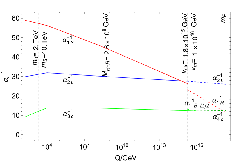
Figure 1: Two loop RG evolution of the gauge couplings for the symmetries $SU(3)_{c}\times SU(2)_{L}\times U(1)_{Y}$, $U(1)_{B-L}$ and $SU(4)_{c}\times SU(2)_{L}\times U(1)_{R}$. Matching conditions at $v_{str}$ are $\alpha^{-1}_{1Y}=\sqrt{3/5}\ \alpha^{-1}_{1R}+\sqrt{2/5}\ \alpha^{-1}_{1(B-L)}$ and $\alpha^{-1}_{2L}=\alpha^{-1}_{2L}$, and at $v_{m}$, $\alpha^{-1}_{3c}=\alpha^{-1}_{4c}=\alpha^{-1}_{1(B-L)}$.

The two loop gauge coupling evolution for the gauge symmetries $SU(4)_{c}\times SU(2)_{L}\times U(1)_{R}$, $SU(3)_{c}\times SU(2)_{L}\times U(1)_{R}\times U(1)_{B-L}$ and $SU(3)_{c}\times SU(2)_{L}\times U(1)_{Y}$ are shown in fig. 1. We have assumed the degeneracy of supersymmetric particles at $m_{S}\simeq 10$ TeV. As discussed below, at MSSM level, a color octet component of the adjoint superfield $\Phi$ with mass $m_{3/2}\simeq 2$ TeV and $H,\overline{H}$ pair with mass $m_{H}\simeq 3\times 10^{8}$ GeV are present.

III Shifted $\mu$-Hybrid Inflation in Supersymmetric $SU(4)_{c}\times SU(2)_{L}\times U(1)_{R}$ Model

In the discussion below, the scalar components of the superfields are denoted by the same symbols as their respective superfields. We express the scalar field $\Phi$ in the $SU(4)_{c}$ adjoint basis $\Phi=\phi_{a}\,T^{a}$, $\text{Tr}[\Phi^{2}]=\phi^{a}\,\phi^{a}/2$, $\text{Tr}[\Phi^{3}]=d^{abc}\,\phi_{a}\,\phi_{b}\,\phi_{c}/4$. Here $d^{abc}=2\,\text{Tr}[T^{a}\,\{T^{b},\,T^{c}\}]$ is totally symmetric and $[T^{b},\,T^{c}]=if^{bcd}\,T^{a}$ with, $f^{bcd}$ being totally antisymmetric. The indices $a,b,c$ run from $1$ to $15$, and the repeated indices are summed over.

The scalar potential obtained from the superpotential in section II is given by

$$V \supset\left|\kappa\,M^{2}-\dfrac{\kappa}{2}\,\phi_{a}\,\phi_{a}-\dfrac{\beta}{M_{\star}}\,\dfrac{d^{abc}}{4}\,\phi_{a}\,\phi_{b}\,\phi_{c}\right|^{2}$$ (6)

$$+\left|S\right|^{2}\,\left|\kappa\,\phi_{a}+\dfrac{3\,\beta}{4\,M_{\star}}\,d^{abc}\,\phi_{b}\,\phi_{c}\right|^{2}+V_{D},$$

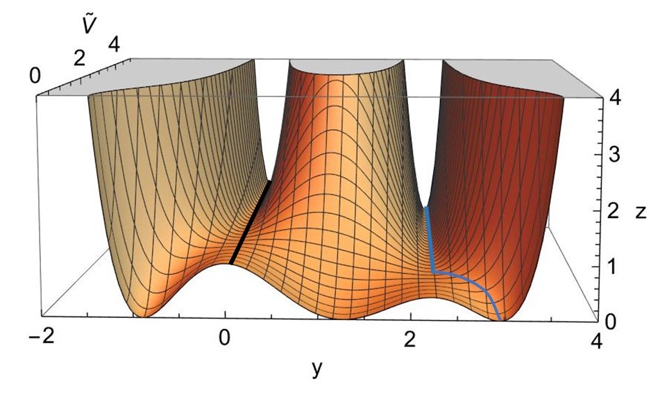
Figure 2: Schematic display of shifted hybrid track for $\xi=0.3$. The two minima at $y=0$ and $y\simeq 2.3$, shown by black and blue color lines, correspond to standard and shifted trajectory respectively.

where $V_{D}$ is the D-term potential given by

$$V_{D}\supset g_{4}^{2}\,\left(f^{abc}\,\phi_{b}\,\phi_{c}^{\star}\right)\,\left(f^{ade}\,\phi_{d}\,\phi_{e}^{\star}\right).$$ (7)

Vanishing of the D-term is achieved by taking, $\phi_{a}=\phi_{15}\,\delta_{a,15}$, where $\phi_{15}$ is chosen to be a real scalar field. In the D-flat direction, we used an appropriate $R$ transformation to rotate the $S$ complex field to the real axis, $S=\sigma/\sqrt{2}$, where $\sigma$ is a canonically normalized real scalar field playing the role of inflaton. The supersymmetric global minimum of the above potential lies at

$$\dfrac{\beta}{2\,\kappa\,M_{\star}}\,d^{abc}\,\phi_{a}^{0}\,\phi_{b}^{0}\,\phi_{c}^{0}+\phi_{a}^{0}\,\phi_{a}^{0}=2\,M^{2},$$ (8)

where the superscript $``0"$ denotes the field value at its global minimum and,

$$\langle S\rangle=\langle h_{u}\rangle=\langle h_{d}\rangle=\langle H\rangle=\langle\overline{H}\rangle=0.$$ (9)

During inflation with $S>M$, the various Higgs fields, namely $h_{u}\,,h_{d}\,,H\,,\overline{H}$, acquire heavy masses, leading them to quickly stabilize at zero. Exploiting the $SU(4)_{c}$ symmetry, the matrix $\Phi^{0}$ can be transformed into a diagonal form as shown in eq. 3. Consequently, eq. 8 takes the following form

$$v^{2}=4\,M^{2}+\frac{\xi\,v^{3}}{2M},$$ (10)

where we have used $d_{15,15,15}=-\sqrt{2/3}$, $\xi=\beta\,M/\sqrt{3}\,\kappa\,M_{\star}$, and only $\phi^{0}_{15}=v/\sqrt{2}\neq 0$.

We can rewrite the scalar potential in eq. 6 in terms of the dimensionless fields

$$y=\dfrac{\phi_{15}}{\sqrt{2}\,M}\,\,\,\,\,\,\text{and}\,\,\,\,\,\,z=\dfrac{\sigma}{\sqrt{2}\,M},$$ (11)

with

$$\tilde{V}\equiv\dfrac{V}{\kappa\,M^{4}}=\left(1-y^{2}+\xi\,y^{3}\right)^{2}+2\,z^{2}\,y^{2}\left(1-3\,\xi\,y/2\right)^{2}.$$ (12)

The schematic display of this potential is shown in fig. 2. Thus, for a constant value of $z$, the local minima for standard (1) and shifted (2) trajectories are

$$y_{1}=0\,\,\,\,\,\text{and}\,\,\,\,\,y_{2}=\dfrac{2}{3\,\xi}.$$ (13)

As explained in [37], the interesting region for the parameter $\xi$ in the current analysis is given by $0.27<\xi<0.38$.

Fields	Squared Masses
2 real scalars	$\kappa^{2}|S|^{2}\pm\kappa^{2}M^{2}(\frac{4}{27\xi^{2}}-1)$
1 Majorana fermion	$\kappa^{2}|S|^{2}$
16 real scalars	$4\kappa^{2}|S|^{2}\pm 2\kappa^{2}M^{2}(\frac{4}{27\xi^{2}}-1)$
8 Majorana fermions	$4\kappa^{2}|S|^{2}$
8 real scalars	$\lambda_{h}^{2}S^{2}\pm\kappa\lambda_{h}m^{2}$
4 Majorana fermions	$\lambda_{h}^{2}S^{2}$
16 real scalars	$\lambda_{H}^{2}S^{2}\pm\kappa\lambda_{H}m^{2}$
8 Majorana fermions	$\lambda_{H}^{2}S^{2}$
6 real scalars	$\frac{2}{3}g^{2}v_{2}^{2}$
6 Dirac fermions	$\frac{2}{3}g^{2}v_{2}^{2}$
6 gauge bosons	$\frac{2}{3}g^{2}v_{2}^{2}$

Table 2: Mass spectrum of the shifted hybrid $SU(4)_{c}$ model as the system moves along the inflationary trajectory $y_{2}$ ($v_{2}=2\,M\,y_{2}=\frac{4\,M}{3\,\xi}$).

In table 2, we summarize the results of the mass spectrum of the model along the shifted inflationary trajectory, $y_{2}=2/(3\xi)$. All these supermultiplets satisfy the supertrace rule $\text{Str}[M^{2}]=0$.

The inflationary effective potential with 1-loop radiative correction is given by

$$V_{\rm 1loop} =\kappa^{2}M_{\xi}^{4}\big{(}1+\frac{\kappa^{2}}{16\,\pi^{2}}\left[F(M_{\xi}^{2},x^{2})+8\times 4\,F(2M_{\xi}^{2},2\,x^{2})\right.\big{.}$$

$$\big{.}\left.+4\gamma^{2}_{h}F(m_{h}^{2},x_{h}^{2})+8\gamma^{2}_{H}F(m_{H}^{2},x_{H}^{2})\right]\big{)}.$$ (14)

Here

$$F(M_{\xi}^{2},x^{2}) =\frac{1}{4}\left(\left(x^{4}+1\right)\ln\frac{\left(x^{4}-1\right)}{x^{4}}+2x^{2}\ln\frac{x^{2}+1}{x^{2}-1}\right.$$

$$\left.+2\ln\frac{\kappa^{2}M_{\xi}^{2}x^{2}}{Q^{2}}-3\right),$$ (15)

where $x=|S|/M_{\xi}$, $M_{\xi}^{2}=M^{2}(4/27\xi^{2}-1)$, $m_{h}^{2}=\gamma_{h}M_{\xi}^{2}$, $x_{h}^{2}=\gamma_{h}x^{2}$ with $\gamma_{h}=\lambda_{h}/\kappa$ and $m_{H}^{2}=\gamma_{H}M_{\xi}^{2}$, $x_{H}^{2}=\gamma_{H}x^{2}$ with $\gamma_{H}=\lambda_{H}/\kappa<<1$ and $Q$ is the renormalization scale. The $SU(3)_{c}$ octet multiplet is massless in the supersymmetric limit as a consequence of both R and the gauge symmetries. This will not be a problem as gauge coupling unification is not a prediction of our model.

IV SUGRA corrections and nonminimal Kähler potential

We take the following general form of the Kähler potential:

$$K= |S|^{2}+Tr|\Phi|^{2}+|H|^{2}+|\bar{H}|^{2}+|h_{u}|^{2}+|h_{d}|^{2}$$

$$+ \kappa_{S\Phi}\frac{|S|^{2}\,Tr|\Phi|^{2}}{m_{P}^{2}}+\kappa_{SH}\frac{|S|^{2}|H|^{2}}{m_{P}^{2}}+\kappa_{S\bar{H}}\frac{|S|^{2}|\bar{H}|^{2}}{m_{P}^{2}}$$

$$+ \kappa_{H\Phi}\frac{|H|^{2}\,Tr|\Phi|^{2}}{m_{P}^{2}}+\kappa_{\bar{H}\Phi}\frac{|\bar{H}|^{2}\,Tr|\Phi|^{2}}{m_{P}^{2}}+\kappa_{H\bar{H}}\frac{|H|^{2}|\bar{H}|^{2}}{m_{P}^{2}}$$

$$+ \kappa_{S}\frac{|S|^{4}}{4m_{P}^{2}}+\kappa_{\Phi}\frac{(Tr|\Phi|^{2})^{2}}{4m_{P}^{2}}+\kappa_{H}\frac{|H|^{4}}{4m_{P}^{2}}+\kappa_{\bar{H}}\frac{|\bar{H}|^{4}}{4m_{P}^{2}}$$

$$+ \kappa_{SS}\frac{|S|^{6}}{6m_{P}^{4}}+\cdots,$$ (16)

where $m_{P}\simeq 2.4\times 10^{18}$ GeV is the reduced Planck mass. Additionally, for the sake of simplicity, the contribution of many other terms e.g., of the form

$$c_{2}\,[Tr(\Phi^{2})+h.c.]+c_{3}\,[Tr(\Phi^{3})/m_{P}+h.c.]+\cdots$$ (17)

is assumed to be zero. Alternatively, we can effectively absorb these extra contributions coming from the $\Phi$ superfield into various couplings of the above Kähler potential as only the $|S|$ field plays an active role during inflation. The sugra scalar potential is given by

$$V_{F}=e^{K/m_{P}^{2}}\left(K_{i\bar{j}}^{-1}D_{z_{i}}WD_{z^{*}_{j}}W^{*}-3m_{P}^{-2}\left|W\right|^{2}\right),$$ (18)

with $z_{i}$ being the bosonic components of the superfields $z_{i}\in\{S,\Phi,H,\bar{H},\cdots\}$ and we have defined

$$D_{z_{i}}W\equiv\frac{\partial W}{\partial z_{i}}+m_{P}^{-2}\frac{\partial K}{\partial z_{i}}W,\,\,\,K_{i\bar{j}}\equiv\frac{\partial^{2}K}{\partial z_{i}\partial z_{j}^{*}},$$ (19)

and $D_{z_{i}^{*}}W^{*}=\left(D_{z_{i}}W\right)^{*}.$ Now in the inflationary trajectory with the D-flat direction ($\phi_{i}=\delta_{i,15}\phi_{15}$, $|\bar{H}_{a}|=|H_{a}|$) and using sections II, 14, 16 and 18. we obtain the following form of the full potential:

$$V=V_{\rm 1loop}+\kappa^{2}M_{\xi}^{4}\left(\left(\frac{4(1-\kappa_{S\Phi})}{9\,(4/27-\xi^{2})}-\kappa_{S}\,x^{2}\right)\right.\left(\frac{M_{\xi}}{m_{P}}\right)^{2}$$

$$\left.+\left(\frac{4((1-2\kappa_{S\Phi})^{2}+1+\kappa_{\Phi})}{81\,(4/27-\xi^{2})^{2}}\right.\right.$$

$$\left.\left.+\frac{4((1-\kappa_{S\Phi})^{2}-\kappa_{S}(1-2\kappa_{S\Phi}))x^{2}}{9\,(4/27-\xi^{2})}\right.\right.$$

$$\left.\left.+\frac{\gamma_{S}\,x^{4}}{2}\right)\left(\frac{M_{\xi}}{m_{P}}\right)^{4}+a\,\dfrac{m_{3/2}}{\sqrt{2}\,\kappa\,M_{\xi}}\,x+\cdots\right)+\cdots\,,$$ (20)

where $x=|S|/M_{\xi}$ and $\gamma_{S}=1-\frac{7\kappa_{S}}{2}+2\kappa_{S}^{2}-3\kappa_{SS}$.

The inflationary slow-roll parameters are given by

$$\epsilon=\frac{m_{P}^{2}}{4\,M_{\xi}^{2}}\left(\frac{\partial_{x}V}{V}\right)^{2},\,\,\,\eta=\frac{m_{P}^{2}}{2\,M_{\xi}^{2}}\left(\frac{\partial_{x}^{2}V}{V}\right).$$ (21)

In the slow-roll approximation (i.e. $\epsilon$, $|\eta|\ll 1$), the scalar spectral index $n_{s}$ and the tensor to scalar ratio $r$ are given (to leading order) by

$$n_{s}\simeq 1+2\,\eta-6\,\epsilon,\,\,\,r\simeq 16\,\epsilon.$$ (22)

The relevant number of e-folds, $N_{0}$, before the end of inflation, is

$$N_{0}=2\left(\frac{M_{\xi}}{m_{P}}\right)^{2}\int_{x_{e}}^{x_{0}}\left(\frac{V}{\partial_{x}V}\right)dx,$$ (23)

where $|S_{0}|=x_{0}\,M_{\xi}$ is the field value at the pivot scale $k_{0}=0.05$ Mpc^-1, and $x_{e}$ denotes the field value at the end of inflation, defined by $|\eta(x_{e})|=1$ (or $x_{e}=1$). During inflation, this scale exits the horizon at approximately

$$N_{0}=53+\frac{1}{3}\ln\left(\frac{T_{r}}{10^{9}~{}{\rm GeV}}\right)+\frac{2}{3}\ln\left(\frac{V^{1/4}(x_{0})}{10^{15}~{}{\rm GeV}}\right),$$ (24)

where $T_{r}$ is the reheat temperature and for the numerical work we will set $T_{r}=2\times 10^{9}$ GeV. This could easily be reduced to lower values if the gravitino problem is considered to be an issue. The amplitude of the curvature perturbation is given by

$$\Delta_{\mathcal{R}}^{2}=\frac{1}{24\,\pi^{2}}\left.\left(\frac{V/m_{P}^{4}}{\epsilon}\right)\right|_{k=k_{0}},$$ (25)

where $\Delta_{\mathcal{R}}^{2}=(2.43\pm 0.11)\times 10^{-9}$ is the Planck 2018 normalization. Note that, for added precision, we include in our calculations the first order corrections [38] in the slow-roll expansion for the quantities $n_{s}$, $r$ and $\Delta_{\mathcal{R}}$.

V Global Minimum and symmetry breaking after Inflation

Note that from the mixing terms in the Kähler potential, $K\supset\left(\kappa_{SH}|S|^{2}|H|^{2}+\kappa_{S\overline{H}}|S|^{2}|\overline{H}|^{2}\right)/m_{P}^{2}$, an effective mass term for $(H,\overline{H})$ is generated in the scalar potential which, in the D-flat direction $|H|=|\overline{H}|$ becomes, $(\kappa^{2}M^{4}/m_{P}^{2})2\beta_{H}|H|^{2}$, with $\beta_{H}=(\kappa_{SH}+\kappa_{S\overline{H}})/2-1$ chosen to be positive. During inflation, the mass term for $(H=\overline{H})$ is

$$\lambda_{H}^{2}S^{2}-\frac{\kappa^{2}M^{4}}{m_{P}^{2}}\beta_{H}>0.$$ (26)

which quickly stabilizes the fields $|H|=|\overline{H}|$ to zero. After the inflationary phase, as the inflaton field value falls below a critical value,

$$S_{c}\equiv\left(\dfrac{\kappa}{\lambda_{H}}\right)\left(\dfrac{M}{m_{P}}\right)\,M\,\sqrt{\beta_{H}},$$ (27)

the fields $|H|=|\overline{H}|$ become unstable and develop a nonzero vev,

$$v_{H}\equiv\langle H\rangle=S_{c}\leq M_{\xi},$$ (28)

with $S_{c}$ given in eq. 27. This process simultaneously triggers the breaking of the underlying symmetry, $U(1)_{R}\times U(1)_{B-L}$, and initiates the formation of a CS network.

The global minimum potential at the end of inflation is

$$\langle\kappa\,M^{2}-\kappa\,Tr[\Phi^{2}]-\dfrac{\beta}{M_{*}}Tr[\Phi^{3}]+\lambda_{H}\,v_{H}^{2}\rangle=0,$$ (29)

and

$$\langle S\rangle=0=\langle h_{u}\,h_{d}\rangle,\,\,\,\,\,\langle H\rangle=v_{H}=\langle\bar{H}\rangle.$$ (30)

For simplicity, we will assume that $\kappa\,M^{2}>>\lambda_{H}\,v_{H}^{2}$ and therefore inflaton primarily acts as a two-field oscillatory system centered around the global vev specified by eq. 29.

The terms in the scalar potential involving the $H\,\bar{H}$ field in the $D$-flat direction are

$$V(H=\bar{H})\supset-2\,\beta_{H}\,\dfrac{\kappa^{2}\,M^{4}}{m_{p}^{2}}\,H^{2}+\lambda_{H}^{2}\,H^{4},$$ (31)

giving the following expression for the mass of $H$ field,

$$M_{H=\bar{H}}=2\sqrt{\beta_{H}}\dfrac{M}{m_{P}}\,\dfrac{m_{\text{inf}}}{(1-3\,\xi\,v/(4\,M))}.$$ (32)

This indicates that $M_{H=\bar{H}}<m_{\text{inf}}$ for $\beta_{H}\leq 1$. Choosing the CS formation at the end of inflation, $S_{c}=M_{\xi}$, implies that, $\lambda_{H}\leq\kappa\,M/m_{P}$ for $\beta_{H}\leq 1$. For $v_{H}\leq M$, we obtain $\lambda_{H}<<\kappa$, leading to a suppression in the decay of the inflaton into $H\bar{H}$. Note that for our benchmark point in table 3 $M_{H=\bar{H}}\simeq 2.6\times 10^{8}$ GeV, which is greater than the Hubble mass, $\mathcal{H}\simeq\kappa\,M_{\xi}^{2}/(\sqrt{3}\,m_{P})\simeq 3.4\times 10^{7}$ GeV. Therefore, there will be no inflation after the formation of the cosmic string network.

VI Inflaton Decay and Reheating

After the end of inflation, the system falls towards the SUSY vacuum and performs damped oscillations about it. The inflaton system consists of the two scalar fields $s$ and $\theta=\delta\phi$ with the same mass,

$$m_{\text{inf}}\simeq\sqrt{2}\kappa\,v\,\left(1-3\,\xi\,v/4M\right).$$ (33)

The inflaton predominantly decays into a pair of higgsinos ($\widetilde{h}_{u}$, $\widetilde{h}_{d}$) and higgses ($h_{u}$, $h_{d}$), each with a decay width, $\Gamma_{h}$, given by,

$$\Gamma_{h}=\Gamma(\theta\rightarrow\widetilde{h}_{u}\widetilde{h}_{d})=\Gamma(S\rightarrow h_{u}h_{d})=\frac{\lambda_{h}^{2}}{8\pi}m_{\text{inf}}.$$ (34)

The other decay mode, via the superpotential couplings $(\gamma_{ij}/M_{*})\,N_{H}^{2}N^{c}_{i}N^{c}_{j}$, leads to a pair of right-handed neutrinos ($N$) and sneutrinos ($\widetilde{N}$) respectively with equal decay width given as,

$$\Gamma_{N} =\Gamma(\theta\rightarrow NN)=\Gamma(s\rightarrow\widetilde{N}\widetilde{N})$$

$$=\dfrac{1}{8\pi}\frac{\lambda_{H}^{2}M^{2}}{m_{\text{inf}}^{2}}\left(\frac{M_{N}}{M}\right)^{2}\left(1-\dfrac{4M_{N}^{2}}{m_{\text{inf}}^{2}}\right)^{1/2},$$ (35)

provided that only the lightest right-handed neutrino with mass $M_{N}$ satisfies the kinematic bound, $m_{\text{inf}}>2M_{N}$. This implies that $\gamma<0.03(\kappa/4.3\times 10^{-5})$. However, this decay mode is very much suppressed due to $\lambda_{H}\ll\kappa$. Inflaton decays to a color octet with mass $\sim m_{3/2}$ is also suppressed.

With $H=3\Gamma_{\text{inf}}$, we define the reheat temperature $T_{r}$ in terms of the inflaton decay width $\Gamma_{\text{inf}}$,

$$T_{r}=\left(\dfrac{90}{\pi^{2}g_{*}}\right)^{1/4}\sqrt{\Gamma_{\text{inf}}\,m_{P}},$$ (36)

where $g_{*}=228.75$ for MSSM and $\Gamma_{\text{inf}}=\Gamma_{h}+\Gamma_{N}\simeq\Gamma_{h}$. Although the $\Gamma_{N}$ channel is important for successful leptogenesis, it is very much suppressed, $\Gamma_{N}\ll\Gamma_{h}$. In fact, for our benchmark point in table 3, we obtain a suppression of $\sim 10^{-2}$. Therefore, leptogenesis is not generated in totality in the present model. Note that one straightforward way to resolve this problem is to invoke split supersymmetry [30] but we will not discuss it here.

Table 3: Benchmark point for metastable cosmic strings.

$T_{r}$	$2\times 10^{9}$ GeV	$M_{\xi}$	$1.8\times 10^{15}$ GeV
$m_{\text{inf}}$	$7\times 10^{9}\,\text{Gev}$	$m_{3/2}$	$2\,\text{Tev}$
$\xi$	$0.3$	$\kappa$	$4.3\times 10^{-5}$
$\kappa_{S}$	$0.0168$	$\kappa_{SS}$	$1$
$\gamma_{h}$	$1$	$N_{0}$	$50$
$n_{s}$	$0.965$	$r$	$1.7\times 10^{-14}$

VII Constraints on Metastable Cosmic Strings

The strength of the string’s gravitational interaction is expressed in terms of the dimensionless string tension, $G\mu_{\text{cs}}$, where $G=1/8\pi m_{P}^{2}$ and $\mu_{\text{cs}}$ is mass per unit length of the string. The CMB bound on the CS tension is [39, 40],

$$G\mu_{\text{cs}}\lesssim 1.3\times 10^{-7}.$$ (37)

The quantity $\mu_{\text{cs}}$, can be written in terms of the $U(1)_{R}\times U(1)_{{B-L}}$ gauge symmetry breaking scale $M_{\xi}$ as $\mu_{\text{cs}}\simeq 2\pi M_{\xi}^{2}$. With $G\mu_{\text{cs}}\lesssim 1.3\times 10^{-7}$ we obtain $M_{\xi}\lesssim 1.8\times 10^{15}$ GeV, and this is possible with a metastable CS network as described in [41]. This possibility not only circumvents the CMB bound on $G\mu_{\text{cs}}$, it can also evade other bounds coming from LIGO O3 [42].

The critical value of $S$ for CS production (also $M_{\text{str}}$) is

$$v_{str}\equiv S_{c}=\frac{\kappa M^{2}}{m_{P}}\frac{\sqrt{\beta_{H}}}{\lambda_{H}}.$$ (38)

Taking $S_{c}=M_{\xi}=M(4/27\xi^{2}-1)^{1/2}$ (end of inflation) we obtain

$$\frac{\kappa M}{m_{P}}=\frac{\lambda_{H}}{\sqrt{\beta_{H}}}(4/27\xi^{2}-1)^{1/2}<<1.$$ (39)

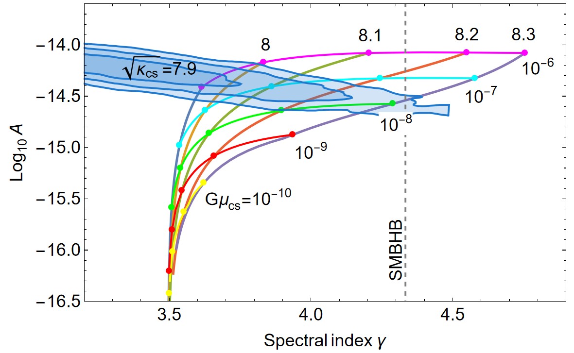
Figure 3: The GWs signal from metastable CSs compared to the NANOGrav observation for different values of $G\mu_{cs}$ and $\sqrt{\kappa_{cs}}$. Moving from top to bottom, $G\mu_{cs}$ varies from $10^{-6}$ to $10^{-10}$, while moving from left to right $\sqrt{\kappa_{cs}}$ varies between $7.9$ to $8.3$. The blue region shows the $3\sigma,2\sigma$ and $1\sigma$ NANOGrav posterior contours [1]. The gray vertical line at $\gamma_{cs}=13/3$ represents the slope expected for supermassive black hole binary (SMBHB) merger.

The metastable string network decays via the Schwinger production of monopole-antimonopole pairs with a rate per string unit length of [43, 41, 44, 45]

$$\Gamma_{d}=\frac{\mu_{cs}}{2\pi}\exp(-\pi\kappa_{\text{cs}}),$$ (40)

where $\kappa_{\text{cs}}$ quantifies the metastability of CSs network and is given by

$$\kappa^{1/2}_{\text{cs}} \sim \frac{M_{m}}{\sqrt{\mu}}\sim\frac{4\pi M_{X}}{g_{m}^{2}}\frac{1}{\sqrt{2\pi}\,v_{str}}.$$ (41)

Here $M_{m}$ is the monopole mass and $M_{X}=\sqrt{2/3}\,(g_{m}v_{m})$ is the gauge boson mass associated with the GUT symmetry breaking responsible for monopole production. For metastable CSs to explain NANOGrav we need $\kappa^{1/2}_{\text{cs}}\sim 8$ [2] and this implies,

$$\frac{v_{m}}{v_{str}}\sim 2\,g_{m},$$ (42)

where $g_{m}=g_{4}(M_{X})=g_{3}(M_{X})$ with $\upsilon_{m}=4\,M/(3\,\xi)\sim 4\,M$ and $v_{str}=M_{\xi}$. Thus, we obtain $v_{m}/M_{\text{str}}\sim 5.6$ implying $g_{m}\sim 2.8$. With minimal matter content, we obtain $g_{m}\sim 1$. However, if we add an additional $15$-plet with light color-octet we can easily obtain the required value of $g_{m}$. The metastable CSs lying within the NANOGrav 15-year posteriors are shown in fig. 3. For our benchmark point in table 3, with $G\mu_{\text{cs}}\simeq 10^{-7}$ and $\kappa_{\text{cs}}\simeq 8.1$, the GW spectrum is shown in fig. 4.

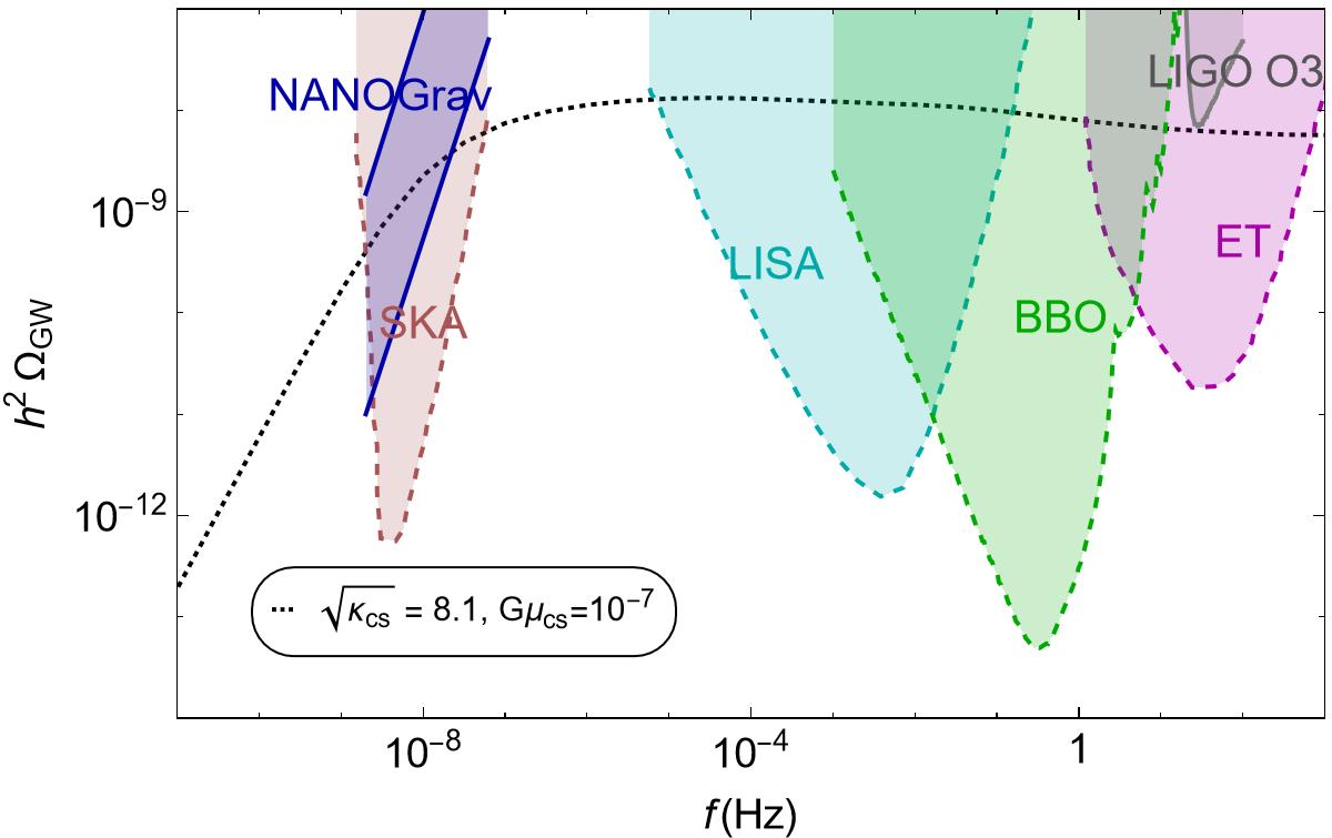
Figure 4: The GW spectrum for our benchmark point table 3, which explains the NANOGrav excess at 2$\sigma$ for $G\mu_{\text{cs}}\simeq 10^{-7}$ and $\sqrt{\kappa_{\text{cs}}}\simeq 8.1$. The gray shaded regions indicate the sensitivity curves of present (solid boundaries) LIGO O3 [42] and future (dashed boundaries) SKA [46], LISA [47], ET [48], BBO [49] experiments.

VIII Conclusions

We have shown that superheavy metastable strings can evade inflation in a supersymmetric model based on the gauge symmetry $SU(4)_{c}\times SU(2)_{L}\times U(1)_{R}$. The strings described here produce a GW spectrum that appears to be compatible with the recent pulsar timing array experiments. Measurements in other frequency ranges should provide additional tests of the model. Moreover, our considerations here can be extended to the breaking chain $SO(10)\rightarrow SU(3)_{c}\times SU(2)_{L}\times U(1)_{Y}\times U(1)_{\chi}\rightarrow SU(3)_{c}\times SU(2)_{L}\times U(1)_{Y}$, previously discussed in [34]. The first breaking produces the $SO(10)$ GUT monopole as well as the ‘$\chi$’ monopole, with the latter being the analog of the ‘red’ monopole in our $SU(4)_{c}\times SU(2)_{L}\times U(1)_{R}$ model. Additional care is required to make sure that the symmetry breaking scales are compatible with the NANOGrav and LIGO- VIRGO measurements.

References

- Agazie et al. [2023] G. Agazie et al. (NANOGrav), Astrophys. J. Lett. 951, L8 (2023), arXiv:2306.16213 [astro-ph.HE] .
- Afzal et al. [2023] A. Afzal et al. (NANOGrav), Astrophys. J. Lett. 951, L11 (2023), arXiv:2306.16219 [astro-ph.HE] .
- Antoniadis et al. [2023] J. Antoniadis et al. (EPTA), (2023), arXiv:2306.16214 [astro-ph.HE] .
- Reardon et al. [2023] D. J. Reardon et al., Astrophys. J. Lett. 951, L6 (2023), arXiv:2306.16215 [astro-ph.HE] .
- Xu et al. [2023] H. Xu et al., Res. Astron. Astrophys. 23, 075024 (2023), arXiv:2306.16216 [astro-ph.HE] .
- Buchmuller et al. [2020a] W. Buchmuller, V. Domcke, and K. Schmitz, Phys. Lett. B 811, 135914 (2020a), arXiv:2009.10649 [astro-ph.CO] .
- Buchmuller et al. [2021] W. Buchmuller, V. Domcke, and K. Schmitz, JCAP 12, 006 (2021), arXiv:2107.04578 [hep-ph] .
- Lazarides et al. [2023a] G. Lazarides, R. Maji, A. Moursy, and Q. Shafi, (2023a), arXiv:2308.07094 [hep-ph] .
- Buchmuller et al. [2023] W. Buchmuller, V. Domcke, and K. Schmitz, (2023), arXiv:2307.04691 [hep-ph] .
- Antusch et al. [2023] S. Antusch, K. Hinze, S. Saad, and J. Steiner, (2023), arXiv:2307.04595 [hep-ph] .
- Ahmed et al. [2023a] W. Ahmed, M. U. Rehman, and U. Zubair, (2023a), arXiv:2308.09125 [hep-ph] .
- Lazarides et al. [2023b] G. Lazarides, R. Maji, and Q. Shafi, (2023b), arXiv:2306.17788 [hep-ph] .
- Lazarides et al. [2023c] G. Lazarides, Q. Shafi, and A. Tiwari, JHEP 05, 119 (2023c), arXiv:2303.15159 [hep-ph] .
- Dvali et al. [1994] G. R. Dvali, Q. Shafi, and R. K. Schaefer, Phys. Rev. Lett. 73, 1886 (1994), arXiv:hep-ph/9406319 .
- Copeland et al. [1994] E. J. Copeland, A. R. Liddle, D. H. Lyth, E. D. Stewart, and D. Wands, Phys. Rev. D 49, 6410 (1994), arXiv:astro-ph/9401011 .
- Senoguz and Shafi [2005] V. N. Senoguz and Q. Shafi, Phys. Rev. D 71, 043514 (2005), arXiv:hep-ph/0412102 .
- Rehman et al. [2010a] M. U. Rehman, Q. Shafi, and J. R. Wickman, Phys. Lett. B 683, 191 (2010a), arXiv:0908.3896 [hep-ph] .
- Buchmuller et al. [2000] W. Buchmuller, L. Covi, and D. Delepine, Phys. Lett. B 491, 183 (2000), arXiv:hep-ph/0006168 .
- Bastero-Gil et al. [2007] M. Bastero-Gil, S. F. King, and Q. Shafi, Phys. Lett. B 651, 345 (2007), arXiv:hep-ph/0604198 .
- ur Rehman et al. [2007] M. ur Rehman, V. N. Senoguz, and Q. Shafi, Phys. Rev. D 75, 043522 (2007), arXiv:hep-ph/0612023 .
- Rehman et al. [2010b] M. U. Rehman, Q. Shafi, and J. R. Wickman, Phys. Lett. B 688, 75 (2010b), arXiv:0912.4737 [hep-ph] .
- Shafi and Wickman [2011] Q. Shafi and J. R. Wickman, Phys. Lett. B 696, 438 (2011), arXiv:1009.5340 [hep-ph] .
- Rehman et al. [2011] M. U. Rehman, Q. Shafi, and J. R. Wickman, Phys. Rev. D 83, 067304 (2011), arXiv:1012.0309 [astro-ph.CO] .
- Civiletti et al. [2011] M. Civiletti, M. U. Rehman, Q. Shafi, and J. R. Wickman, Phys. Rev. D 84, 103505 (2011), arXiv:1104.4143 [astro-ph.CO] .
- Buchmüller et al. [2014] W. Buchmüller, V. Domcke, K. Kamada, and K. Schmitz, JCAP 07, 054 (2014), arXiv:1404.1832 [hep-ph] .
- Buchmuller [2021] W. Buchmuller, JHEP 04, 168 (2021), arXiv:2102.08923 [hep-ph] .
- Ahmed et al. [2022] W. Ahmed, M. Junaid, S. Nasri, and U. Zubair, Phys. Rev. D 105, 115008 (2022), arXiv:2202.06216 [hep-ph] .
- Ahmed et al. [2023b] W. Ahmed, M. Moosa, S. Munir, and U. Zubair, JHEP 05, 011 (2023b), arXiv:2208.11888 [hep-ph] .
- Masoud et al. [2021] M. A. Masoud, M. U. Rehman, and Q. Shafi, JCAP 11, 022 (2021), arXiv:2107.09689 [hep-ph] .
- Okada and Shafi [2017] N. Okada and Q. Shafi, Phys. Lett. B 775, 348 (2017), arXiv:1506.01410 [hep-ph] .
- Rehman et al. [2017] M. U. Rehman, Q. Shafi, and F. K. Vardag, Phys. Rev. D 96, 063527 (2017), arXiv:1705.03693 [hep-ph] .
- Okada and Shafi [2018] N. Okada and Q. Shafi, Phys. Lett. B 787, 141 (2018), arXiv:1709.04610 [hep-ph] .
- Ahmed et al. [2021] W. Ahmed, A. Karozas, and G. K. Leontaris, Phys.Rev.D 104, 055025 (2021), arXiv:2104.04328 [hep-ph] .
- Afzal et al. [2022] A. Afzal, W. Ahmed, M. U. Rehman, and Q. Shafi, Phys. Rev. D 105, 103539 (2022), arXiv:2202.07386 [hep-ph] .
- Lazarides and Shafi [2019] G. Lazarides and Q. Shafi, JHEP 10, 193 (2019), arXiv:1904.06880 [hep-ph] .
- Lazarides et al. [2021] G. Lazarides, M. U. Rehman, Q. Shafi, and F. K. Vardag, Phys. Rev. D 103, 035033 (2021), arXiv:2007.01474 [hep-ph] .
- Khalil et al. [2011] S. Khalil, M. U. Rehman, Q. Shafi, and E. A. Zaakouk, Phys. Rev. D 83, 063522 (2011), arXiv:1010.3657 [hep-ph] .
- Senoguz and Shafi [2008] V. N. Senoguz and Q. Shafi, Phys. Lett. B 668, 6 (2008), arXiv:0806.2798 [hep-ph] .
- Aghanim et al. [2020] N. Aghanim et al. (Planck), Astron. Astrophys. 641, A6 (2020), [Erratum: Astron.Astrophys. 652, C4 (2021)], arXiv:1807.06209 [astro-ph.CO] .
- Akrami et al. [2020] Y. Akrami et al. (Planck), Astron. Astrophys. 641, A10 (2020), arXiv:1807.06211 [astro-ph.CO] .
- Buchmuller et al. [2020b] W. Buchmuller, V. Domcke, H. Murayama, and K. Schmitz, Phys. Lett. B 809, 135764 (2020b), arXiv:1912.03695 [hep-ph] .
- Abbott et al. [2021] R. Abbott et al. (KAGRA, Virgo, LIGO Scientific), Phys. Rev. D 104, 022004 (2021), arXiv:2101.12130 [gr-qc] .
- Monin and Voloshin [2010] A. Monin and M. B. Voloshin, Phys. Atom. Nucl. 73, 703 (2010), arXiv:0902.0407 [hep-th] .
- Monin and Voloshin [2008] A. Monin and M. B. Voloshin, Phys. Rev. D 78, 065048 (2008).
- Leblond et al. [2009] L. Leblond, B. Shlaer, and X. Siemens, Phys. Rev. D 79, 123519 (2009).
- Smits et al. [2009] R. Smits, M. Kramer, B. Stappers, D. R. Lorimer, J. Cordes, and A. Faulkner, Astron. Astrophys. 493, 1161 (2009), arXiv:0811.0211 [astro-ph] .
- Pau Amaro-Seoane, et al. [2017] Pau Amaro-Seoane, et al., (2017), arXiv:1702.00786 [astro-ph.IM] .
- Punturo et al. [2010] M. Punturo et al., Class. Quant. Grav. 27, 194002 (2010).
- Corbin and Cornish [2006] V. Corbin and N. J. Cornish, Class. Quant. Grav. 23, 2435 (2006), arXiv:gr-qc/0512039 .