Pigeons.jl: Distributed sampling from intractable distributions
Abstract
We introduce a software package, Pigeons.jl, that provides a way to leverage distributed computation to obtain samples from complicated probability distributions, such as multimodal posteriors arising in Bayesian inference and high-dimensional distributions in statistical mechanics. Pigeons.jl provides simple APIs to perform such computations single-threaded, multi-threaded, and/or distributed over thousands of MPI-communicating machines. In addition, Pigeons.jl guarantees a property that we call strong parallelism invariance: the output for a given seed is identical irrespective of the number of threads and processes, which is crucial for scientific reproducibility and software validation. We describe the key features of Pigeons.jl and the approach taken to implement a distributed and randomized algorithm that satisfies strong parallelism invariance.
keywords:
Distributed computation, Bayesian inference, parallelism invariance, multi-threading, Message Passing Interface, Markov chain Monte Carlo1 Introduction
In many scientific application domains, the ability to obtain samples from a distribution is crucial. For instance, sampling methods have been used to discover magnetic polarization in the black hole of galaxy M87 [2] and to image the Sagittarius A* black hole [1]. They have also been used to model the evolution of single-cell cancer genomes [22], infer plasma dynamics inside nuclear fusion reactors [13], and to identify gerrymandering in Georgia’s 2021 congressional districting plan [31]. Similarly, evaluating high-dimensional integrals or sums over complicated combinatorial spaces are related tasks that can also be solved with sampling via Markov chain Monte Carlo (MCMC) methods. However, such calculations can often be bottlenecks in the scientific process, with simulations that can last days or even weeks to finish.
Pigeons.jl111The source code for Pigeons.jl can be found at https://github.com/Julia-Tempering/Pigeons.jl. Pigeons.jl v0.2.0, used in the example scripts below, is currently compatible with Julia 1.8+. enables users to sample efficiently from high-dimensional and complex distributions and solve integration problems by implementing state-of-the-art sampling algorithms [27, 26] that leverage distributed computation. Its simple API allows users to perform such computations single-threaded, multi-threaded, and/or distributed over thousands of MPI-communicating machines. Further, it comes with guarantees on strong parallelism invariance wherein the output for a given seed is identical irrespective of the number of threads or processes. Such a level of reproducibility is rare in distributed software but of great use for the purposes of debugging in the context of sampling algorithms, which produce stochastic output. Specifically, Pigeons.jl is designed to be suitable and yield reproducible output for:
-
1.
one machine running on one thread;
-
2.
one machine running on several threads;
-
3.
several machines running, each using one thread, and
-
4.
several machines running, each using several threads.
1.1 Problem formulation
We describe the class of problems that can be approached using Pigeons.jl. Let denote a probability density 222This density may also be a probability mass function (discrete variables). We also allow for a combination of discrete/continuous variables. called the target. In many problems, e.g. in Bayesian statistics, the density is typically known only up to a normalizing constant,
| (2) |
where can be evaluated pointwise but is typically unknown. Pigeons.jl takes as input the function .
The output of Pigeons.jl can be used for two main tasks:
-
1.
Approximating integrals of the form . For example, the choice computes the mean and computes the probability of under , where denotes the indicator function.
-
2.
Approximating the value of the normalization constant . For example, in Bayesian statistics, this corresponds to the marginal likelihood, which can be used for model selection.
Its implementation shines compared to traditional sampling packages in the following scenarios:
-
•
When the target density is challenging due to a complex structure (e.g., high-dimensional, multi-modal, etc.).
-
•
When the user needs not only but also the normalization constant . Many existing tools focus on the former and struggle or fail to do the latter.
-
•
When the target distribution is defined over a non-standard space, e.g. a combinatorial object such as a phylogenetic tree.
1.2 What is of interest to the general Julia developer?
Ensuring code correctness at the intersection of randomized, parallel, and distributed algorithms is a challenge. To address this challenge, we designed Pigeons.jl based on a principle that we refer to as strong parallelism invariance (SPI). Namely, the output of Pigeons.jl is completely invariant to the number of machines and/or threads. Without explicitly keeping SPI in mind during software construction, the (random) output of the algorithm is only guaranteed to have the same distribution. This is a much weaker guarantee that, in particular, makes debugging difficult. However, with our notion of SPI we make debugging and software validation considerably easier. This is because the developer can first focus on the fully serial randomized algorithm, and then use it as an easy-to-compare gold-standard reference for parallel/distributed implementations. This strategy is used extensively in Pigeons.jl to ensure correctness. In contrast, testing equality in distribution, while possible (e.g., see [12]), incurs additional false negatives due to statistical error.
The general Julia developer will be interested in:
-
•
The main causes of a violation of strong parallelism invariance that we have identified (Section 4)—some of which are specific to Julia—and how we address them in Pigeons.jl.
-
•
The SplittableRandoms.jl333https://github.com/Julia-Tempering/SplittableRandoms.jl package that was developed by our team to achieve strong parallelism invariance in Pigeons.jl (Section 4.2).
2 Examples
In this section we present a set of minimal examples that demonstrate how to use Pigeons.jl for sampling. For further reading, we also direct readers to our growing list of examples, which can be found at https://github.com/Julia-Tempering/Pigeons.jl/tree/main/examples. We begin by installing the latest official release of Pigeons.jl: {lstlisting}[language = Julia] using Pkg; Pkg.add("Pigeons")
2.1 Targets
To use Pigeons.jl, we must specify a target distribution, given by in Eq. 2. Numerous possible types of target distributions are supported, including custom probability densities (specified up to a normalizing constant) written in Julia. We also allow to interface with models written in common probabilistic programming languages, including:
-
•
Turing.jl [11] models (TuringLogPotential)
-
•
Stan [9] models (StanLogPotential)
-
•
Comrade.jl444https://github.com/ptiede/Comrade.jl models for black hole imaging (ComradeLogPotential)
-
•
Non-Julian models with foreign-language Markov chain Monte Carlo (MCMC) code (e.g. Blang [4] code for phylogenetic inference over combinatorial spaces)
Additional targets are currently being accommodated and will be introduced to Pigeons.jl in the near future.
In what follows, we demonstrate how to use Pigeons with a Julia Turing model applied to a non-identifiable “coinflip” data set, modified from the example at https://turing.ml/v0.22/docs/using-turing/quick-start. The Bayesian model can be formulated as
| (3) | ||||
| (4) |
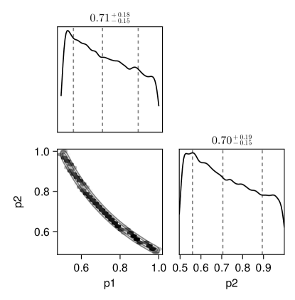
The random variable is the number of heads observed on coin flips where the probability of heads is . This model is non-identifiable, meaning that it is not possible to distinguish the effects of the two different parameters and . As a consequence, the target distribution exhibits a complicated structure, as displayed in Fig. 1. The density of interest corresponding to this model is
| (5) |
where
| (6) | ||||
| (7) |
The distribution is also known as the posterior distribution in Bayesian statistics.
Suppose that we perform coin tosses and observe heads. We would like to obtain samples from our posterior, , having collected this data. We begin by installing Turing {lstlisting}[language = Julia] Pkg.add("Turing") and then defining our Turing model and storing it in the variable model: {lstlisting}[language = Julia] using Turing @model function coinflip(n, y) p1 Uniform(0.0, 1.0) p2 Uniform(0.0, 1.0) y Binomial(n, p1 * p2) return y end model = coinflip(100000, 50000)
From here, it is straightforward to sample from the density given by Eq. 6 up to a normalizing constant. We use non-reversible parallel tempering [27] (PT), Pigeons.jl’s state-of-the-art sampling algorithm, to sample from the target distribution. PT comes with several tuning parameters and [27] describe how to select these parameters effectively, which Pigeons.jl implements under the hood. We also specify that we would like to store the obtained samples in memory to be able to produce trace-plots, as well as some basic online summary statistics of the target distribution and useful diagnostic output by specifying record = [traces, online, round_trip, Pigeons.timing_extrema, Pigeons.allocation_extrema]. It is also possible to leave the record argument empty and reasonable defaults will be selected for the user. The code below runs Pigeons.jl on one machine with one thread. We use the default values for most settings, however we explain later how one can obtain improved performance by setting arguments more carefully (see Section 2.4). {lstlisting}[language = Julia] using Pigeons pt = pigeons( target = TuringLogPotential(model), record = [ traces, online, round_trip, Pigeons.timing_extrema, Pigeons.allocation_extrema]) Note that to convert the Turing model into an appropriate Pigeons.jl target for sampling, we pass the model as an argument to TuringLogPotential(). Once we have stored the PT output in the variable pt we can access the results, as described in the following section. The standard output after running the above code chunk is displayed in Fig. 2 and explained in the next section. For purposes of comparison, we also run a traditional (single-chain Markov chain Monte Carlo) method.
————————————————————————————– #scans restarts Λ time(s) allc(B) log(Z₁/Z₀) min(α) mean(α) ———- ———- ———- ———- ———- ———- ———- ——— 2 0 1.04 0.383 3.48e+07 -4.24e+03 0 0.885 4 0 4.06 0.00287 1.79e+06 -16.3 4.63e-06 0.549 8 0 3.49 0.00622 3.55e+06 -12.1 0.215 0.612 16 0 2.68 0.0161 7.46e+06 -10.2 0.518 0.703 32 0 4.29 0.0353 1.37e+07 -11.8 0.222 0.524 64 3 3.17 0.0699 2.86e+07 -11.5 0.529 0.648 128 8 3.56 0.139 5.53e+07 -11.5 0.523 0.605 256 12 3.38 0.241 1.1e+08 -11.6 0.526 0.625 512 37 3.48 0.473 2.22e+08 -12 0.527 0.614 1.02e+03 77 3.55 0.895 4.46e+08 -11.8 0.571 0.605 ————————————————————————————–
2.1.1 Other targets
As mentioned previously, it is also possible to specify targets with custom probability densities, as well as Stan and Turing models. Additionally, suppose we have some code implementing vanilla MCMC, written in an arbitrary “foreign” language such as C++, Python, R, Java, etc. Surprisingly, it is very simple to bridge such code with Pigeons.jl. The only requirement on the foreign language is that it supports reading the standard input and writing to the standard output, as described in our online documentation.
2.2 Outputs
Pigeons.jl provides many useful types of output, such as: plots of samples from the distribution, estimates of normalization constants, summary statistics of the target distribution, and various other diagnostics. We describe several examples of possible output below.
2.2.1 Standard output
An example of the standard output provided by Pigeons.jl is displayed in Fig. 2. Each row of the table in the output indicates a new tuning round in parallel tempering, with the #scans column indicating the number of scans/samples in that tuning round. During these tuning rounds, Pigeons.jl searches for optimal values of certain PT tuning parameters. Other outputs include:
-
•
restarts: a higher number is better. Informally, PT performs well at sampling from high-dimensional and/or multi-modal distributions by pushing samples from an easy-to-sample distribution (the reference) to the more difficult target distribution. A tempered restart happens when a sample from the reference successfully percolates to the target. (See the subsequent sections for a more detailed description of parallel tempering.) When the reference supports i.i.d. sampling, tempered restarts can enable large jumps in the state space.
-
•
: the global communication barrier, as described in [27], which measures the inherent difficulty of the sampling problem. A rule of thumb to configure the number of PT chains is also given by [27], where they suggest that stable performance should be achieved when the number of chains is set to roughly 2. See Section 2.2.6 for more information.
-
•
time and allc: the time (in seconds) and number of allocations (in bytes) used in each round.
-
•
: an estimate of the logarithm of the ratio of normalization constants between the target and the reference. In many cases, .
-
•
min() and mean(): minimum and average swap acceptance rates during the communication phase across the PT chains. See Section 3 for a description of PT communication.
2.2.2 Plots
It is straightforward to obtain plots of samples from the target distribution, such as trace-plots, pairwise plots, and density plots of the marginals.
To obtain posterior densities and trace-plots, we first make sure that we have the third-party MCMCChains.jl555https://github.com/TuringLang/MCMCChains.jl, StatsPlots.jl666https://github.com/JuliaPlots/StatsPlots.jl, and PlotlyJS.jl777https://github.com/JuliaPlots/PlotlyJS.jl packages installed via {lstlisting}[language=Julia] Pkg.add("MCMCChains", "StatsPlots", "PlotlyJS")
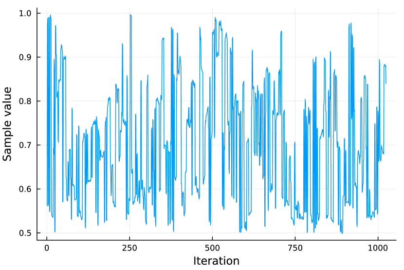
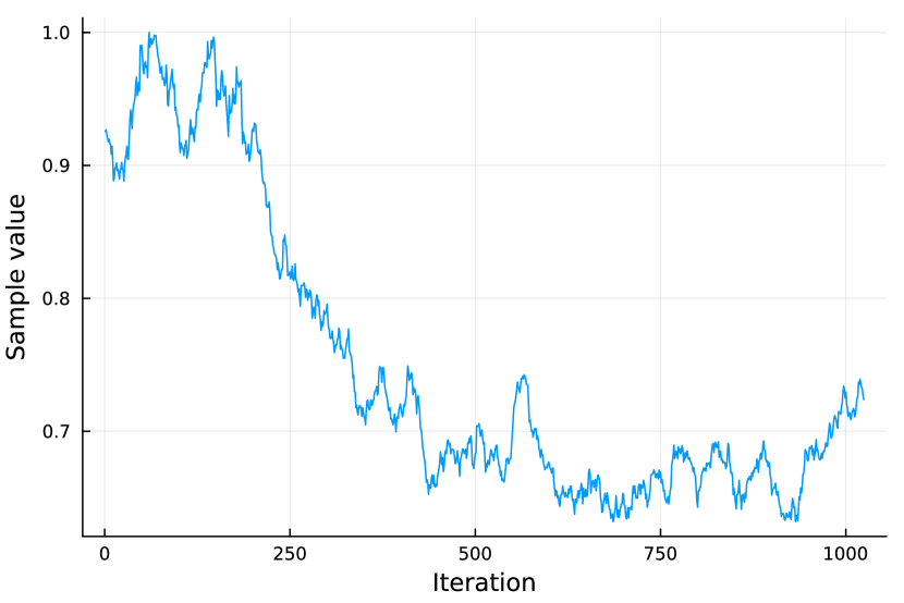
With the pt output object from before for our non-identifiable coinflip model, we can run the following: {lstlisting}[language=Julia] using MCMCChains, StatsPlots, PlotlyJS plotlyjs() samples = Chains( sample_array(pt), variable_names(pt)) my_plot = StatsPlots.plot(samples) display(my_plot) The output of the above code chunk is an interactive plot that can be zoomed in or out and exported as an HTML webpage. A modified static version of the output for the first parameter, , is displayed in the top panel of Fig. 3, along with a comparison to the output from a single-chain algorithm in the bottom panel of the same figure.
To obtain pair plots, we add the PairPlots.jl888https://github.com/sefffal/PairPlots.jl and CairoMakie.jl999https://github.com/JuliaPlots/CairoMakie.jl packages: {lstlisting}[language=Julia] Pkg.add("PairPlots", "CairoMakie") and then run {lstlisting}[language=Julia] using PairPlots, CairoMakie my_plot = PairPlots.pairplot(samples) display(my_plot) The output of the above code chunk with an increased number of samples is displayed in Fig. 1. 101010The code chunk above only works with Julia 1.9.
2.2.3 Estimate of normalization constant
The (typically unknown) constant in Eq. 2 is referred to as the normalization constant. In many applications, it is useful to approximate this constant. For example, in Bayesian statistics, this corresponds to the marginal likelihood and can be used for model selection.
As a side-product of PT, we automatically obtain an approximation to the natural logarithm of the normalization constant. This is done automatically using the stepping stone estimator [30]. The estimate can be accessed using {lstlisting}[language=Julia] stepping_stone(pt) In the case of the normalization constant given by Eq. 7 for and , we can exactly obtain its value as using a computer algebra system. Note that this is very close to the output provided in Fig. 2.
2.2.4 Online statistics
Having specified the use of the online recorder in our call to pigeons(), we can output some basic summary statistics of the marginals of our target distribution. For instance, it is straightforward to estimate the mean and variance of each of the marginals of the target with {lstlisting}[language=Julia] using Statistics mean(pt); var(pt) Other constant-memory statistic accumulators are made available in the OnlineStats.jl [10] package. To add additional constant-memory statistic accumulators, we can register them via Pigeons.register_online_type(), as described in our online documentation. For instance, we can also compute constant-memory estimates of extrema of our distribution.
2.2.5 Off-memory processing
When either the dimensionality of the model or the number of samples is large, the obtained samples may not fit in memory. In some cases it may be necessary to store samples to disk if our statistics of interest cannot be calculated online and with constant-memory (see Section 2.2.4). We show here how to save samples to disk when Pigeons.jl is run on a single machine. A similar interface can be used over MPI.
First, we make sure that we set checkpoint = true, which saves a snapshot at the end of each round in the directory results/all/<unique directory> and is symlinked to results/latest. Second, we make sure that we use the disk recorder by setting record = [disk], along with possibly any other desired recorders. Accessing the samples from disk can then be achieved in a simple way using the Pigeons.jl function process_sample().
2.2.6 PT diagnostics
We describe how to produce some key parallel tempering diagnostics from [27].
The global communication barrier, denoted in Pigeons.jl output, can be used to approximately inform the appropriate number of chains. Based on [27], stable PT performance should be achieved when the number of chains is set to roughly . This can be achieved by modifying the n_chains argument in the call to pigeons(). The global communication barrier is shown at each round and can also be accessed with {lstlisting}[language=Julia] Pigeons.global_barrier(pt)
The number of restarts per round can be accessed with {lstlisting}[language=Julia] n_tempered_restarts(pt) These quantities are also displayed in Fig. 2. Many other useful PT diagnostic statistics and plots can be obtained, as described in our full documentation.
2.3 Parallel and distributed PT
One of the main benefits of Pigeons.jl is that it allows users to easily parallelize and/or distribute their PT sampling efforts. We explain how to run MPI locally on one machine and also how to use MPI when a cluster is available.
2.3.1 Running MPI locally
To run MPI locally on one machine using four MPI processes and one thread per process, use {lstlisting}[language = Julia] pigeons( target = TuringLogPotential(model), on = ChildProcess( n_local_mpi_processes = 4, n_threads = 1))
2.3.2 Running MPI on a cluster
Often, MPI is available via a cluster scheduling system. To run MPI over several machines:
-
1.
In the cluster login node, follow the Pigeons.jl installation instructions in our online documentation.
-
2.
Start Julia in the login node, and perform a one-time setup by calling Pigeons.setup_mpi().
-
3.
In the Julia REPL running in the login node, run:
[language = Julia] pigeons( target = TuringLogPotential(model), n_chains = 1_000, on = MPI(n_mpi_processes = 1_000, n_threads = 1)) The code above will start a distributed PT algorithm with 1,000 chains on 1,000 MPI processes each using one thread. Note that for the above code chunks involving ChildProcess() and MPI() to work, it may be necessary to specify dependencies in their function calls.
2.4 Additional options
In the preceding example we only specified the target distribution and let Pigeons.jl decide on default values for most other settings of the inference engine. There are various settings we can change, including: the random seed (seed), the number of PT chains (n_chains), the number of PT tuning rounds/samples (n_rounds), and a variational reference distribution family (variational), among other settings. For instance, we can run {lstlisting}[language = Julia] pigeons( target = TuringLogPotential(model), n_rounds = 10, n_chains = 10, variational = GaussianReference(), seed = 2 ) which runs PT with the same Turing model target as before and explicitly states that we should use 10 PT tuning rounds with 10 chains (described below). In the above code chunk we also specify that we would like to use a Gaussian variational reference distribution. That is, the reference distribution is chosen from a multivariate Gaussian family that lies as close as possible to the target distribution in order to improve the efficiency of PT. We refer readers to [26] for more details. When only continuous parameters are of interest, we encourage users to consider using variational = GaussianReference() and setting n_chains_variational = 10, for example, as the number of restarts may substantially increase with these settings.
3 Parallel tempering
Pigeons.jl provides an implementation of distributed parallel tempering (PT) described in [27], which we outline in Algorithm 1. This section gives both a brief overview of PT and some details of its distributed implementation.
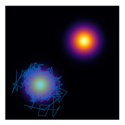
In this section we assume a basic understanding of Markov chain Monte Carlo (MCMC) methods. For readers unfamiliar with MCMC, it is important to know that it is a method to obtain approximate samples from a distribution. More specifically, it is a class of algorithms for simulating a Markov chain of states that look like draws from the target distribution . However, with traditional MCMC methods, the samples may be heavily correlated instead of independent and may fail to sufficiently explore the full space of the distribution (see Fig. 4); PT is a method that aims to address these issues. For a more in-depth review of PT, we refer readers to [26].
3.1 Overview of PT
Suppose that we would like to estimate integrals involving , such as . These integrals may be multivariate and even include combinations of continuous and discrete variables (where sums replace integrals in the discrete case). One method is to obtain samples from to approximate such integrals. Often, the distribution can be challenging for traditional MCMC methods—such as Metropolis-Hastings, slice sampling, and Hamiltonian Monte Carlo— because of its structure. For example, in a bimodal example such as the one illustrated in Figure 4, traditional methods might remain in one of the two modes for an extremely long period of time.
To resolve this issue, PT constructs a sequence of distributions, , where is usually equal to . The distributions are chosen so that it is easy to obtain samples from with the sampling difficulty increasing as one approches . An example of such a sequence of distributions, referred to as an annealing path, is shown in Figure 5.


We now turn to explain how this path of distributions can be used to enhance sampling from the target distribution, . PT operates by first obtaining samples from each distribution on the path in parallel (referred to as an exploration phase). Then, samples between adjacent distributions are swapped (referred to as a communication phase). The communication phase in PT is crucial: it allows for the discovery of new regions of the space of the target distribution such as the top-right mode of the distribution presented in Figure 4.
3.2 Local exploration and communication
A struct that is useful for the implementation of PT is the Replica, which we will often refer to in the remainder of this section. A single Replica struct stores a state variable and a chain integer, among other entries. At the beginning of PT, Replicas are created, one for each distribution on the annealing path, and the chain entries in the replicas are initialized at , respectively. For a given Replica, if the chain number is and the state is , then this means that the sample corresponding to the -th distribution in the sequence is currently at location .
In the local exploration phase, each Replica’s state is modified using an MCMC move targeting , where is given by Replica.chain. The MCMC move can either modify Replica.state in-place, or modify the Replica’s state field. This operation is indicated by the local_exploration function in Algorithm 1.
In the communication phase, PT proposes swaps between pairs of replicas. In principle, there are two equivalent ways to do a swap. In the first implementation, the Replicas could exchange their state fields. Alternatively, they could exchange their chain fields. Because we provide distributed implementations, we use the latter as it ensures that the amount of data that needs to be exchanged between two machines during a swap can be made very small (two floating point numbers), resuling in an exchange of messages of size . Note that this cost does not vary with the dimensionality of the state space, in contrast to the first implementation that would transmit messages of size , where is the dimension of the state space, incurring a potentially very high communication cost for large values of .
3.3 Distributed implementation
A distributed implementation of PT is presented in Algorithm 1 and we describe the details of the implementation below. We present the algorithm from the perspective that the number of machines available is equal to the number of Replicas and distributions, . However, Pigeons.jl also allows for the more general case where the number of machines is not necessarily equal to .
3.3.1 The PermutedDistributedArray
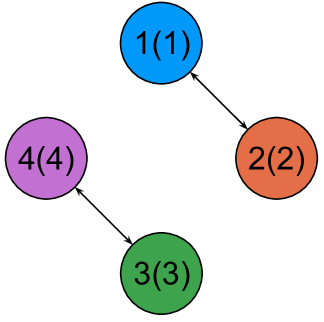
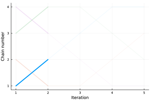
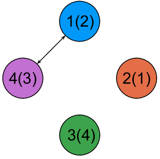
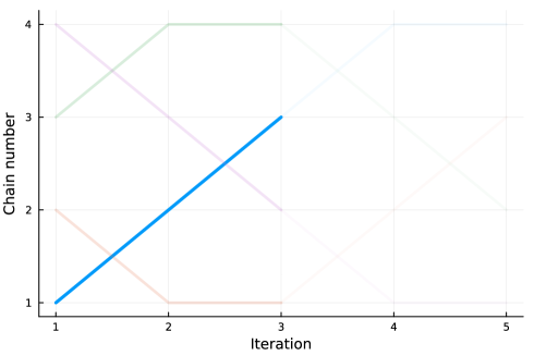
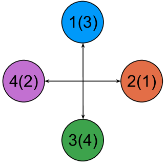
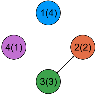
Recall that our theoretical message size for communication between two machines is achieved by exchanging chain indices between Replicas instead of their states. One difficulty can be encountered in a distributed implementation, which we illustrate with the following simple example. Suppose we have distributions, chains, replicas, and machines, and that machine 1 is exploring chain 2 while machine 4 is exploring chain 3. At one point, the Replica at chain 2 (machine 1) might need to exchange chain indices with the Replica that has chain index 3 (machine 4). However, a priori it is not clear how machine 1 should know that it should communicate with machine 4 because it has no knowledge about the chain indices on the other machines.
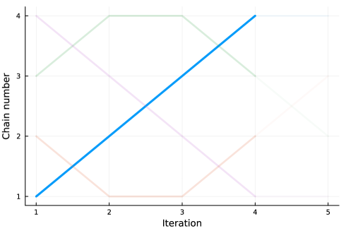
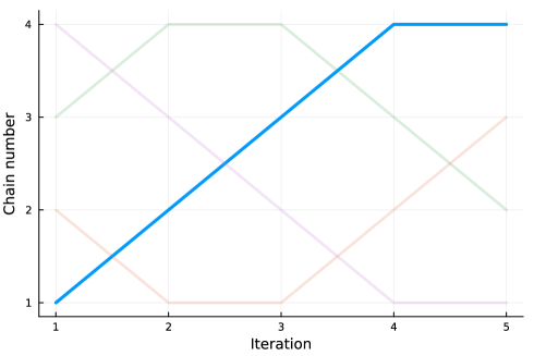
To resolve this issue, we introduce a special data structure called a PermutedDistributedArray. In the case where the number of replicas is equal to the number of available machines, the construction is quite simple and effectively results in each machine storing one additional integer. Considering the same example above, the solution to the problem is to have machine 1 (chain 2 wanting to communicate with chain 3) communicate with machine 3. Machine 3 stores in its dist_array variable of type PermutedDistributedArray the value 4, which is the machine number that stores chain 3. By updating these PermutedDistributedArray variables at each communication step, we can ensure that each machine is aware of which machine number currently stores chain . Therefore, the machines act as keys in a dictionary for the communication permutations. An illustration of communication between four machines is provided in Fig. 6. We note that with a PermutedDistributedArray we make special assumptions on how we access and write to the array elements. Several MPI processes cooperate, with each machine storing data for a slice of this distributed array, and at each time step an index of the array is manipulated by exactly one machine.
3.3.2 MPI implementation details
We use the MPI.jl [7] package to support communication between machines. In our pseudocode in Algorithm 1 we define the MPI-style functions send(), receive!(), and waitall(). The function send() has three arguments in our pseudocode: the first argument is the object to be sent, the second is the machine number to which the object should be sent, and finally the third argument is a unique tag for this specific send/receive request at this time step and on this machine, generated by tag(). The tag() function can be any function that allows one to uniquely identify a tag for a given send/receive request on a given machine at any given time step . The function receive!() has the same last two arguments as send() except that the first argument specifies the object to which data should be written directly. Finally, waitall(requests) waits for all initialized MPI requests for a given pair of machines to complete.
In Algorithm 1 we also introduce the functions permuted_get() and permuted_set!(). Given the current machine’s dist_array and the partner chain with which it should communicate, permuted_get() returns the machine number that holds the partner chain. Given the current machine’s dist_array, chain number, and machine number , permuted_set!() updates the PermutedDistributedArray variables with the updated permutation.
4 Strong parallelism invariance
In this section we describe potential violations of strong parallelism invariance (SPI) that can occur in a distributed setting. We also explain how we avoid these issues by using special distributed reduction schemes and splittable random number generators. Insights provided in this section can be applied to general distributed software beyond Julia.
We have identified two factors that can cause violations of our previously-defined SPI that standard Julia libraries do not automatically take care of:
-
1.
Non-associativity of floating point operations: When several workers perform distributed reduction of floating point values, the output of this reduction will be slightly different depending on the order taken during reduction. When these reductions are then fed into further random operations, this implies that two randomized algorithms with the same seed but using a different number of workers will eventually arbitrarily diverge.
-
2.
Global, thread-local, and task-local random number generators: These are the dominant approaches to parallel random number generators in current languages, and an appropriate understanding of these RNGs is necessary. In particular, in Julia it is important to understand the behaviour of the @threads macro.
Our focus in the remainder of this section is to describe how our implementation solves the two above issues.
4.1 Distributed reduction and floating point non-associativity
After each round of PT, the machines need to exchange information such as the average swap acceptance probabilities, statistics to adapt a variational reference and adjust annealing parameters, and so on. For instance, suppose our state is univariate and real-valued and that each Replica keeps track of the number of times the target chain is visited as well as the mean of the univariate states from the target chain. To obtain the final estimate of the mean of the target distribution, we would like to pool the mean estimates from each of the Replicas, weighted by the number of times that each Replica visited the target chain. This process involves summing floating-point values that are located on each of the Replicas/machines and is an example of a reduction scheme.
To illustrate why distributed reduction with floating point values can violate strong parallelism invariance if not properly implemented, we consider the following toy example. Suppose we have 8 machines storing the floating point numbers , as illustrated in Fig. 7, where we use in the following examples. In this case, if our reduction procedure is to sum the floating point numbers, we know that our final answer should be approximately . However, depending on the exact order in which floating point addition is carried out, the answers might not all be the same and exactly equal to . For instance, in Fig. 7 we see that the order of operations for eight machines would be given by
| (8) | |||
| (9) |
In contrast, with two machines, one possible order of operations might be
| (10) | |||
| (11) |
A possible reduction tree for two machines is illustrated in Fig. 8.
To avoid the issue of non-associativity of floating point arithmetic, we ensure that the order in which operations are performed is exactly the same, irrespective of the number of processes/machines and threads. This is achieved by making sure that every value to be added—if addition is our reduction operation—is a leaf node in the reduction tree, irrespective of the number of machines available to perform the reduction. For instance, if values are to be reduced, then the reduction tree would have leaf nodes. If machines are available, these machines are then assigned in such a way that the order of operations is as if there were machines available. To do so, it may be necessary for a machine to “communicate with itself”, imitating the behaviour that would be present if there were machines available. Fig. 9 and Fig. 10 illustrate the reduction procedure for eight and two machines, respectively.
for tree = circle, draw, minimum size = 0.8cm [ [ [ [] [] ] [ [] [] ] ] [ [ [] [] ] [ [] [] ] ] ]
for tree = circle, draw, minimum size = 0.8cm [ [ [ [ [] [] ] [] ] [] ] [ [] [ [] [ [] [] ] ] ] ]
for tree = circle, draw, minimum size = 0.8cm [, fill = julia1 [, fill = julia1 [, fill = julia1 [, fill = julia1] [, fill = julia2] ] [, fill = julia3 [, fill = julia3] [, fill = julia4] ] ] [, fill = julia5 [, fill = julia5 [, fill = julia5] [, fill = julia6] ] [, fill = julia7 [, fill = julia7] [, fill = julia8] ] ] ]
for tree = circle, draw, minimum size = 0.8cm [, fill = julia1 [, fill = julia1 [, fill = julia1 [, fill = julia1] [, fill = julia1] ] [, fill = julia1 [, fill = julia1] [, fill = julia1] ] ] [, fill = julia2 [, fill = julia2 [, fill = julia2] [, fill = julia2] ] [, fill = julia2 [, fill = julia2] [, fill = julia2] ] ] ]
4.2 Splittable random streams
Another building block towards achieving SPI is a splittable random stream [17, 6]. Julia uses task-local random number generators, a notion that is related to (but does not necessarily imply) strong parallelism invariance. A task is a unit of work on a machine. A task-local RNG would then mean that a separate RNG is used for each unit of work, hopefully implying strong parallelism invariance if the number of tasks is assumed to be constant. Unfortunately, this is not the case when a separate task is created for each thread of execution in Julia. We note that the @threads macro in Julia creates nthreads() tasks and thus nthreads() pseudorandom number generators. This can break strong parallelism invariance as the output may depend on the number of threads.
To motivate splittable random streams, consider the following toy example that violates our notion of SPI: {lstlisting}[language = Julia] using Random import Base.Threads.@threads
println("Num. of threads: (last(result))") With eight threads, this outputs: {lstlisting}[language = Julia] Num. of threads: 8 Result: 0.25679999169092793 Julia guarantees that if we rerun this code, as long as we are using eight threads, we will always get the same result, irrespective of the multi-threading scheduling decisions implied by the @threads-loop. Internally, Julia works with task-local RNGs and the @threads macro spawns nthreads() number of task-local RNGs. For this reason, with a different number of threads, the result is different: {lstlisting}[language = Julia] Num. of threads: 1 Result: 0.8785201210435906
In this simple example above, the difference in output is perhaps not too concerning, but for our parallel tempering use case, the distributed version of the algorithm is significantly more complex and difficult to debug compared to the single-threaded one. We therefore take task-local random number generation one step further and achieve SPI, which guarantees that the output is not only reproducible with respect to repetitions for a fixed number of threads, but also for different numbers of threads or processes.
A first step to achieve this is to associate one random number generator to each Replica. To do so, we use our SplittableRandoms.jl package, which is a Julia implementation of Java SplittableRandoms. Our package offers an implementation of SplitMix64 [25], which allows us to turn one seed into an arbitrary collection of pseudo-independent RNGs. A quick example of how to use the SplittableRandoms.jl library is given below. By splitting a master RNG using the split() function, we can achieve SPI even with the use of the @threads macro.
[language = Julia] using Random using SplittableRandoms: SplittableRandom, split import Base.Threads.@threads
println("Num. of threads: (last(result))") With one and eight threads, the code above outputs {lstlisting}[language = Julia] Num. of threads: 1 Result: 0.4394633333251359 {lstlisting}[language = Julia] Num. of threads: 8 Result: 0.4394633333251359
5 Related work
Automated software packages for Bayesian inference have revolutionized Bayesian data analysis in the past two decades, and are now a core part of a typical applied statistics workflow. For example, packages such as BUGS [19, 20, 21], JAGS [14], Stan [9], PyMC3 [23], and Turing.jl [11] have been widely used in many scientific applications.
These software packages often provide two key user-facing components: (1) a probabilistic programming language (PPL), which allows users to specify Bayesian statistical models in code with a familiar, mathematics-like syntax; and (2) an inference engine, which is responsible for performing computational Bayesian inference once the model and data have been specified. Pigeons.jl focuses on the development of a new inference engine that employs distributed, high-performance computing.
Inference engines available in existing software packages are varied in their capabilities and limitations. For instance, the widely-used Stan inference engine is only capable of handling real-valued (i.e., continuous) parameters. Other tools, such as JAGS, are capable of handling discrete-valued parameters but are limited in their capability to handle custom data-types (e.g. phylogenetic trees). Of those that have the capability to model arbitrary data types, none have an automatically distributed implementation to our knowledge. Turing.jl [11] offers another popular inference engine and PPL, however Pigeons.jl allows one to interface with several different PPLs as well as to easily perform distributed computation.
There is also a vast literature on distributed and parallel Bayesian inference algorithms [3, 5, 8, 16, 15, 18, 24, 28, 29, 32]. These methods unfortunately do not lead to widely usable software packages because they either introduce unknown amounts of approximation error, involve significant communication cost, or reduce the generality of Bayesian inference.
6 Conclusion
Pigeons.jl is a Julia package that enables users with no experience in distributed computing to efficiently approximate posterior distributions and solve challenging Lebesgue integration problems over a distributed computing environment. The core algorithm behind Pigeons.jl is distributed, non-reversible parallel tempering [27, 26]. Pigeons.jl can be used in a multi-threaded context, as well as distributed over up to thousands of MPI-communicating machines. Further, Pigeons.jl is designed so that for a given seed, the output is identical regardless of the number of threads or processes used.
7 Acknowledgements
NS acknowledges the support of a Vanier Canada Graduate Scholarship. PT acknowledges the support of the Black Hole Initiative at Harvard University, which is funded by grants from the John Templeton Foundation and the Gordon and Betty Moore Foundation to Harvard University. PT also acknowledges support by the National Science Foundation grants AST-1935980 and AST-2034306 and the Gordon and Betty Moore Foundation (GBMF-10423). SS acknowledges the support of EPSRC grant EP/R034710/1 CoSines. ABC and TC acknowledge the support of an NSERC Discovery Grant. We also acknowledge use of the ARC Sockeye computing platform from the University of British Columbia, as well as cloud computing resources provided by Oracle.
References
- [1] Kazunori Akiyama, Antxon Alberdi, Walter Alef, Juan Carlos Algaba, Richard Anantua, Keiichi Asada, Rebecca Azulay, Uwe Bach, Anne-Kathrin Baczko, David Ball, et al. First Sagittarius A* Event Horizon Telescope results. IV. Variability, morphology, and black hole mass. The Astrophysical Journal Letters, 930(2):L15, 2022.
- [2] Kazunori Akiyama, Juan Carlos Algaba, Antxon Alberdi, Walter Alef, Richard Anantua, Keiichi Asada, Rebecca Azulay, Anne-Kathrin Baczko, David Ball, Mislav Baloković, et al. First M87 Event Horizon Telescope results. VII. Polarization of the ring. The Astrophysical Journal Letters, 910(1):L12, 2021.
- [3] Rémi Bardenet, Arnaud Doucet, and Chris Holmes. On Markov chain Monte Carlo methods for tall data. The Journal of Machine Learning Research, 18(1):1515–1557, 2017.
- [4] Alexandre Bouchard-Côté, Kevin Chern, Davor Cubranic, Sahand Hosseini, Justin Hume, Matteo Lepur, Zihui Ouyang, and Giorgio Sgarbi. Blang: Bayesian declarative modeling of general data structures and inference via algorithms based on distribution continua. Journal of Statistical Software, 103:1–98, 2022.
- [5] Anthony E Brockwell. Parallel Markov chain Monte Carlo simulation by pre-fetching. Journal of Computational and Graphical Statistics, 15(1):246–261, 2006.
- [6] F. Warren Burton and Rex L. Page. Distributed random number generation. Journal of Functional Programming, 2(2):203–212, 1992.
- [7] Simon Byrne, Lucas C Wilcox, and Valentin Churavy. MPI.jl: Julia bindings for the Message Passing Interface. In Proceedings of the JuliaCon Conferences, volume 1, page 68, 2021.
- [8] Ben Calderhead. A general construction for parallelizing Metropolis-Hastings algorithms. Proceedings of the National Academy of Sciences, 111(49):17408–17413, 2014.
- [9] Bob Carpenter, Andrew Gelman, Matthew D Hoffman, Daniel Lee, Ben Goodrich, Michael Betancourt, Marcus Brubaker, Jiqiang Guo, Peter Li, and Allen Riddell. Stan: a probabilistic programming language. Journal of Statistical Software, 76(1), 2017.
- [10] Josh Day and Hua Zhou. OnlineStats.jl: A Julia package for statistics on data streams. Journal of Open Source Software, 5(46), 2020.
- [11] Hong Ge, Kai Xu, and Zoubin Ghahramani. Turing: a language for flexible probabilistic inference. In International Conference on Artificial Intelligence and Statistics, pages 1682–1690. PMLR, 2018.
- [12] John Geweke. Getting it right: joint distribution tests of posterior simulators. Journal of the American Statistical Association, 99(467):799–804, 2004.
- [13] H Gota, MW Binderbauer, T Tajima, A Smirnov, S Putvinski, M Tuszewski, SA Dettrick, DK Gupta, S Korepanov, RM Magee, et al. Overview of C-2W: high temperature, steady-state beam-driven field-reversed configuration plasmas. Nuclear Fusion, 61(10):106039, 2021.
- [14] Kurt Hornik, Friedrich Leisch, Achim Zeileis, and M Plummer. JAGS: a program for analysis of Bayesian graphical models using Gibbs sampling. In Proceedings of the 3rd International Workshop on Distributed Statistical Computing, volume 2, 2003.
- [15] Pierre Jacob, Christian P Robert, and Murray H Smith. Using parallel computation to improve independent Metropolis–Hastings based estimation. Journal of Computational and Graphical Statistics, 20(3):616–635, 2011.
- [16] Pierre E Jacob, John O’Leary, and Yves F Atchadé. Unbiased Markov chain Monte Carlo methods with couplings. Journal of the Royal Statistical Society: Series B (Statistical Methodology), 82(3):543–600, 2020.
- [17] P. L’Ecuyer. Efficient and portable combined random number generators. Communications of the ACM, 31(6):742–751, June 1988.
- [18] Anthony Lee, Christopher Yau, Michael B Giles, Arnaud Doucet, and Christopher C Holmes. On the utility of graphics cards to perform massively parallel simulation of advanced Monte Carlo methods. Journal of Computational and Graphical Statistics, 19(4):769–789, 2010.
- [19] David Lunn, Christopher Jackson, Nicky Best, Andrew Thomas, and David Spiegelhalter. The BUGS Book: A Practical Introduction to Bayesian Analysis. CRC Press, 2013.
- [20] David Lunn, David Spiegelhalter, Andrew Thomas, and Nicky Best. The BUGS project: evolution, critique and future directions. Statistics in Medicine, 28(25):3049–3067, 2009.
- [21] David J Lunn, Andrew Thomas, Nicky Best, and David Spiegelhalter. WinBUGS — a Bayesian modelling framework: concepts, structure, and extensibility. Statistics and Computing, 10:325–337, 2000.
- [22] Sohrab Salehi, Farhia Kabeer, Nicholas Ceglia, Mirela Andronescu, Marc J Williams, Kieran R Campbell, Tehmina Masud, Beixi Wang, Justina Biele, Jazmine Brimhall, et al. Clonal fitness inferred from time-series modelling of single-cell cancer genomes. Nature, 595(7868):585–590, 2021.
- [23] John Salvatier, Thomas V Wiecki, and Christopher Fonnesbeck. Probabilistic programming in Python using PyMC3. PeerJ Computer Science, 2:e55, 2016.
- [24] Steven L Scott, Alexander W Blocker, Fernando V Bonassi, Hugh A Chipman, Edward I George, and Robert E McCulloch. Bayes and big data: the consensus Monte Carlo algorithm. International Journal of Management Science and Engineering Management, 11(2):78–88, 2016.
- [25] Guy L Steele Jr, Doug Lea, and Christine H Flood. Fast splittable pseudorandom number generators. ACM SIGPLAN Notices, 49(10):453–472, 2014.
- [26] Nikola Surjanovic, Saifuddin Syed, Alexandre Bouchard-Côté, and Trevor Campbell. Parallel tempering with a variational reference. In Advances in Neural Information Processing Systems, 2022.
- [27] Saifuddin Syed, Alexandre Bouchard-Côté, George Deligiannidis, and Arnaud Doucet. Non-reversible parallel tempering: a scalable highly parallel MCMC scheme. Journal of Royal Statistical Society, Series B, 84:321–350, 2021.
- [28] Xiangyu Wang, Fangjian Guo, Katherine A Heller, and David B Dunson. Parallelizing MCMC with random partition trees. Advances in Neural Information Processing Systems, 28, 2015.
- [29] Changye Wu and Christian P Robert. Average of recentered parallel MCMC for big data. arXiv:1706.04780, 2017.
- [30] Wangang Xie, Paul O Lewis, Yu Fan, Lynn Kuo, and Ming-Hui Chen. Improving marginal likelihood estimation for Bayesian phylogenetic model selection. Systematic Biology, 60(2):150–160, 2011.
- [31] Zhanzhan Zhao, Cyrus Hettle, Swati Gupta, Jonathan Christopher Mattingly, Dana Randall, and Gregory Joseph Herschlag. Mathematically quantifying non-responsiveness of the 2021 Georgia congressional districting plan. In EAAMO ‘22: Equity and Access in Algorithms, Mechanisms, and Optimization, pages 1–11, 2022.
- [32] Jun Zhu, Jianfei Chen, Wenbo Hu, and Bo Zhang. Big learning with Bayesian methods. National Science Review, 4(4):627–651, 2017.