Event-based Agile Object Catching with a Quadrupedal Robot
Abstract
Quadrupedal robots are conquering various applications in indoor and outdoor environments due to their capability to navigate challenging uneven terrains. Exteroceptive information greatly enhances this capability since perceiving their surroundings allows them to adapt their controller and thus achieve higher levels of robustness. However, sensors such as LiDARs and RGB cameras do not provide sufficient information to quickly and precisely react in a highly dynamic environment since they suffer from a bandwidth-latency tradeoff. They require significant bandwidth at high frame rates while featuring significant perceptual latency at lower frame rates, thereby limiting their versatility on resource constrained platforms. In this work, we tackle this problem by equipping our quadruped with an event camera, which does not suffer from this tradeoff due to its asynchronous and sparse operation. In leveraging the low latency of the events, we push the limits of quadruped agility and demonstrate high-speed ball catching for the first time. We show that our quadruped equipped with an event-camera can catch objects with speeds up to 15 m/s from 4 meters, with a success rate of 83%. Using a VGA event camera, our method runs at 100 Hz on an NVIDIA Jetson Orin.
Multi-Media Material
For visual results, see our video at https://youtu.be/FpsVB8EO54M. Also check out open-source code at https://github.com/uzh-rpg/event-based_object_catching_anymal.
I Introduction
Humans and animals can perform highly agile maneuvers, which require a combination of fast and precise perception and robust and accurate control. For years roboticists have been inspired by nature and aimed at emulating these capabilities in robotic systems. Recently, quadrupedal robots are reaching animal-like performance on challenging locomotion tasks with exteroception — such as taking a hike in the Alps [1] — and are capable of performing complex maneuvers like recovering from a flipped position [2].
In addition to robust control, many animals also have special retinas with which they perceive their environment, enabling them to perform highly complex maneuvers like a dog catching a frisbee in mid-air. Exteroceptive sensors like LiDARs and RGB cameras have enhanced robots’ perception capabilities and enabled more smooth and complex behaviors. However, despite these advancements, current quadruped robots are still far from achieving the same level of agility as animals like cats and dogs. Indeed, high-speed object catching with onboard sensing remains a significant challenge for quadrupedal robots.
Object catching has been studied with standard RGB cameras [3]. However, it still suffers from fundamental limitations due to the bandwidth-latency tradeoff. High frame rates are necessary to react quickly, but these incur high bandwidths. By contrast, lowering the frame rate increases perceptual latency and can severely impact the robot’s reaction time and success rate. Animal vision systems do not suffer from this tradeoff since they do not perceive their environment as a sequence of frames. Event cameras are neuromorphic sensors that try to emulate the working principle of these systems, and are therefore also not affected by this tradeoff. They only measure changes in intensity which they transmit as asynchronous, binary spikes with micro-second level latency. They have been successfully used in high-speed object evasion with drones [4, 5]. However, it remains unclear how policies devised for quadrotors can be applied to different robotic platforms such as quadrupeds. In this work, we fill this gap, by developing a modular approach to high-speed object catching using an event camera on a quadruped platform equipped with a net, seen in Fig. LABEL:fig:eyecatcher.
Our approach works by first detecting independently moving objects in the event stream, and then fusing these detections to a ballistic parabolic trajectory estimate. This estimate is then processed by a data-driven control policy to perform the catching maneuver. By using events, our approach enjoys a minimal latency, while benefiting from an expressive data-driven policy for catching objects arriving at different angles. Our contributions are the following:
-
•
We present a method for high-speed ball catching from event-based object trajectory estimations. By leveraging the low latency of events we can track objects at up to 100 Hz on an NVIDIA Jetson Orin.
-
•
We are the first to demonstrate successful event camera-based high-speed object catching with a quadrupedal robot equipped with a net. Our policy catches objects flying at up to 15 m/s from 4 meters with an 83% success rate.
-
•
We extend the latency analysis in [6] to estimate object trajectories from detections, and the incurred latencies for standard and event camera-based algorithms.
II Related Work
II-A Dynamic Object Catching in Robotics
Early work on dynamic object catching focused on the case where the object trajectory is fully observable and known and has shown successful implementation on a variety of robotics platforms ranging from robotic arms [7] to drones [8]. Object trajectories in these cases were detected by a motion capture rig using IR markers. Later work showed successful object catching with onboard perception on a drone [3], however, due to the use of a standard camera, objects speeds were limited to 6 m/s, and the vision task was simplified by mounting bright LED lights on the balls. To date, the work by Falanga et al. [6] targets the fastest moving objects, flying at up to 10 m/s with a drone. However, it focuses on object evasion, instead of catching, which puts a lower constraint on the robot policy. By contrast, high-speed object catching, the target of this work, requires precise and agile maneuvering of the robot. The work in [9] is the first to address this task with a linear slider, showing promising results with a learning-based detector. In this work, we take the next step and apply this concept to a complex, legged robot.
II-B Advancements in Legged Robotics
In contrast to the highly maneuverable, lightweight, and easily modeled quadcopters used for onboard catching scenarios in the previous section, legged robots pose a much more sophisticated control problem due to its size and more complex interaction with the environment. A typical approach to control this is to use a model-based controller to plan its motion through a physical model and minimize the objective function such as target velocity error. This often requires computational heavy planning, making it challenging to achieve fast and reactive motion [10, 11, 12]. Recently, a deep reinforcement learning method showed a great capability in complex and agile maneuvers without compromising real-time performance [13, 14, 15, 16, 1]. Utilizing the exteroceptive information was mostly from a separate mapping pipeline which fuses information from the depth sensors [17, 18, 19]. However, this approach poses large latency and makes it difficult to handle dynamic environment. Recently, the attempt of using raw depth images for locomotion task is pursued [20, 21], however, achieving a high-speed visual task in a dynamic environment such as catching a flying object with on-board vision is still an open question. Off-board approaches have already shown promising results: a recent work demonstrated a small quadruped capable of acting as a goalie using a hierarchical reinforcement learning approach, choosing different behaviors based on incoming ball trajectories [22].
III Worst Case Latency Analysis
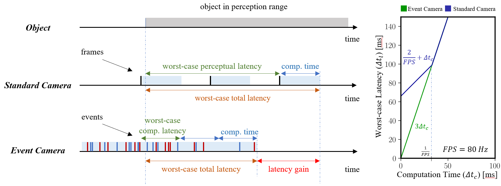
As stated in the introduction, event cameras do not suffer from a latency-bandwidth tradeoff, as do RGB cameras. In this section we will clarify this point, by studying the worst-case latency incurred by algorithms operating on images or events. We will assume that the goal of is to find the parabola describing the ballistic trajectory of the object to be caught, and that this parabola is estimated via a sequence of 3D position and/or 3D velocity measurements. We measure the latency of as the worst-case waiting period to collect a minimum number of measurements that describe the parabola. In this work, we focus on two-shot methods, that require two consecutive 3D position measurements but discuss the potentially interesting class of one-shot methods that measure 3D position and velocity simultaneously and can therefore be even faster. We will discuss the latency considerations for two-shot algorithms designed for standard cameras and event cameras next, summarized in Fig. 1.
Standard camera Algorithms for processing standard images fall in the category of two-shot methods, since single images do not carry motion information. We assume a camera with inter-frame time interval and an algorithm with processing time . In the worst case the robot has to wait a period before it can execute a detection because it has to wait for the next frame to arrive, or a previous detection cycle to terminate (see Fig. 1 middle). Then it can initiate two consecutive detections, which together take , where the first and second term measure the latency for detecting on the first and second frame respectively. If the computation time is lower than the framerate, the detector still needs to wait until the second frame arrives, so its latency is lower-bounded by . As a result, the algorithm has a worst-case latency
| (1) |
Event Camera For an event-based algorithm , so the initial waiting period before detection can start is dominated by a previous detection cycle (see Fig. 1 bottom). In that case, the total worst-case latency becomes
| (2) |
However, since events also carry motion information, an algorithm may try to simultaneously extract 3D position and velocity, and thus this latency can be reduced to . As a result, an event-based algorithm can have lower latency when the following conditions are satisfied
| (3) | |||
| (4) |
In the next section we present a two-shot approach to object catching, and thus our method will benefit more from a fast execution time, outperforming RGB camera-based approaches for similar inter-frame intervals. We leave the study of one-shot approaches for future work.
IV Approach
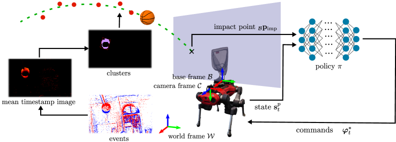
Our object-catching algorithm consists of two main components: A visual frontend, which is tasked with object trajectory estimation based on event-based visual input, and a planning backend that converts the predicted trajectory to low-level motor commands for the quadruped robot. Our full method is illustrated in Fig. 2 and described further below.
IV-A Visual Frontend
Our trajectory estimator is inspired by the moving object detector used in [4], followed by trajectory fitting and filtering steps. For completeness, we will briefly summarize the method below.
Moving Object Detection: Our estimator takes in measurements by an Inertial Measurement Unit (IMU) and a rolling buffer of asynchronous events from a monocular event camera, where each event corresponds to a brightness change measurement at pixel , time and sign .
We then compute the motion compensated mean timestamp image, , using the average of the angular rate measurements by the IMU over the duration of the event buffer. is defined as
| (5) | ||||
Where the represent motion compensated coordinates, with calibration matrix . For events that are well explained by a pure rotation, such as when events are triggered in the background, will be small, while for independently moving objects, will feature higher values. By thresholding we can thus segment out independently moving objects in the image plane resulting in the binary map:
| (6) |
Where is a suitable normalization of the mean timestamp image by its mean, and time window. We use an adaptive threshold, which depends on the angular rate since higher angular rates will cause a higher average . Having identified pixels of moving objects, we fit maximal rectangles around them by employing the DBSCAN clustering algorithm [23]. DBSCAN works by minimizing a dissimilarity score between pixels assigned to the same cluster. We use the same formulation as in [4] which minimizes
| (7) | |||||
where and are pairs of pixels. Similar to [4] we also use optical flow similarity as a criterion. We compute it by using dense Lucas Kanade optical flow on consecutive mean timestamp images . The resulting output of DBSCAN is a set of clusters that we circumscribe with bounding boxes before going to the trajectory estimation step.
Trajectory Estimation
Our next step consists of finding the impact point of the object in the plane perpendicular to the robot, which is used by the planner to execute the catching maneuver. To do this we continuously estimate the ballistic trajectory of the object, from noisy 3D position measurements during observation. While the bounding boxes described above provide us with direction estimates for each point along the parabola, the depth is unobserved for monocular setups. We, therefore, assume a known object size with which we can calculate the object depth according to
| (8) |
where and are the width of the object in the real world and image plane respectively, and is the focal length of the camera. As a result, we can recover the 3D positions of the objects in the camera frame by back-projecting the ray of the center of the bounding box by a depth , and transform it to the fixed world frame with a known transformation from the robot’s odometry. We next fit a parabola of the form
| (9) |
through these 3D points. In the world frame, gravity is . Since these points contain outliers, we use RANSAC to remove them. We successively select random pairs of 3D points, for which we find a solution for and . For each solution we construct the parabola and count the 3D points within a weighted euclidean distance of the parabola, i.e. inliers, satisfying
| (10) | |||
| (11) |
where is the inlier threshold, rotates vectors from camera to world frame, and correspond to variances in , , and direction respectively. Since our 3D object detector exhibit higher noise in the camera -direction, we select and . We select the minimal solution that yields the highest number of inliers, and then fit a and which minimizes the square euclidean distance to the inlier points.
| (12) |
which has a closed-form solution.
Impact Point Estimation The backend controller expects an estimate of the target position of the net which can catch the object. To estimate this position, we calculate the intersecting point of the parabola trajectory and a plane which is spanned in the gravity vector and the y-axis of the robot base. The base frame is centered on the body of the robot and visualized in Fig. 2. We choose to share the origin of . Points on this plane satisfy the relation
| (13) |
with Substituting the parabola equation (9), expressed in body frame and solving for , we can find the time to impact, and the impact point as:
| (14) |
To further improve robustness, we apply a median filter to the series of impact point detections, until the robot initiates the catching maneuver.
IV-B Robot Locomotion Backend
For object catching, we train a policy that controls each joint of a quadrupedal robot to reach with a net mounted on the robot as fast as possible. We model this catching problem as an Markov Decision Process (MDP) and use reinforcement learning to solve it in order to achieve agile behavior with low calculation latency. The objective of reinforcement learning is to maximize a discounted sum of rewards over a finite time horizon, i.e. finding
| (15) |
with discount factor , termination time , and reward function . We used Proximal Policy Optimization (PPO) [24] to train the policy.
 |
 |
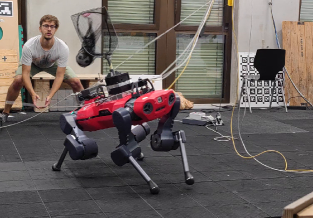 |
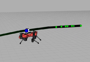
| (a) observed events | (b) estimated parabola | (c) catching maneuver |
States, Action space and Policy We use ANYmal C [25] as a quadrupedal robot model and use the actuator net [13] which simulates the dynamics of the actuator. A policy outputs joint level action that is the differences between the desired and nominal joint position. At each discrete time step it takes as input the state defined as
| (16) |
It comprises the impact point expressed in the body frame of the robot, and proprioceptive states defined as
| (17) |
where is the gravity expressed in the base frame, and represents body linear velocity and angular velocity, and are the joint position and velocity respectively, and is the previous action.
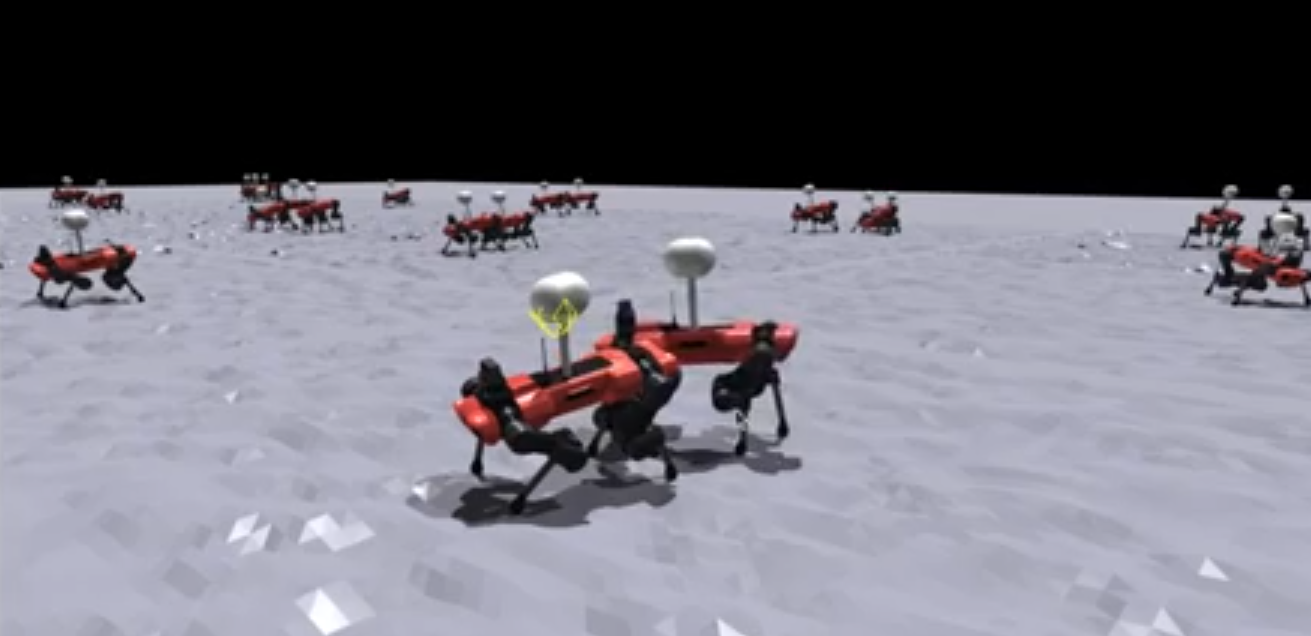
Environment setup We use Isaac gym [26] to build the simulation environment and leverage the highly parallelized implementation on a Graphics Processing Unit (GPU) [27]. In the simulation environment, we spawn a quadrupedal robot equipped with a net on terrain and randomly sample target net position (Fig. 3). The target net position is randomly sampled around the current net position within the range of cm on the x-axis, cm on the y-axis, and cm on the z-axis in the robot base frame. We resample the target net position every 1.0 seconds with a probability of 0.2. To make the policy robust to noisy sensor readings and unexpected foot trapping, we add noise to the observation and a slight roughness to the terrain as seen in Fig. 3. The maximum episode length is 20 sec and we terminate the episode when the robot base or thigh hits the ground.
Rewards
To make the policy track the target net position, we used the following rewards.
Target tracking :
In addition, we have the following penalty rewards to make the motion smooth.
Base linear velocity:
Base angular velocity:
Joint velocity:
Joint acceleration:
Joint torque:
Action difference:
Base orientation:
The final reward is defined as follows by checking the behavior of the policy.
| (18) | |||||
V Experiments
Hardware setup We directly deploy the policy learnt in simulation on the real robot, finding that it required no additional fine-tuning to run in the real world. We use the ANYmal C quadruped robot [25], coupled with a VGA resolution event camera, an IniVation DVXplorer [28], fitted with a field-of-view (FoV) objective. For catching, a landing net with a diameter of m was mounted on the quadruped with its center being m above the base frame. The detection algorithm runs on an NVIDIA Jetson Orin developer kit and
the catching policy was deployed on the robot’s onboard PC, an Intel core i7 8850H with 6 cores and 12 threads. To display the debugging visualization, two Ethernet cables were attached to the laptop PC, but all compute necessary to execute the catching maneuver is running on board. With this hardware setup, our vision algorithm is capable of running at up to 100 Hz.
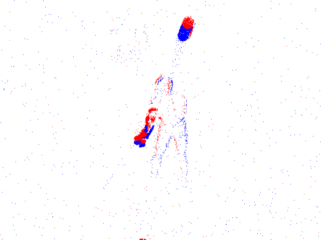
We test the catching pipeline by throwing balls manually in a cluttered environment. To test texture generalization, two different rubber balls were used, each with a diameter of cm. The balls were thrown manually at average speeds between m/s, with net center deviations in the range of m. At these speeds, the incidence angle of the ball was around with respect to the net. A preview of the experiments, including event camera and parabola visualization can be viewed in Fig. 4
Evaluation Proceedure We validate our method by measuring two forms of success rate, one for the vision algorithm, and one to evaluate the overall performance of the system. In the first, we measure the percentage of impact point measurements that have an error lower than the net radius and report the results of this experiment in Tab. II. To evaluate the overall performance we report the percentage of successful catches within a working range of 0.6 m from the initial net position and study the success rate for different throw speeds and deviations from the initial net center. We selected this working range, since beyond it, ANYmal needs to perform significant sideways locomotion, instead of lunging, which slows down the maneuver. These results are summarized in Tab. I. We collect data for a total of 22 throws, for which the ball enters the feasible range of 0.6 m from the robot. While estimated impact points were measured in our visualization (see Fig. 4), measurements of ball speeds and impact points in the real world were measured using footage from a 60 fps external camera.
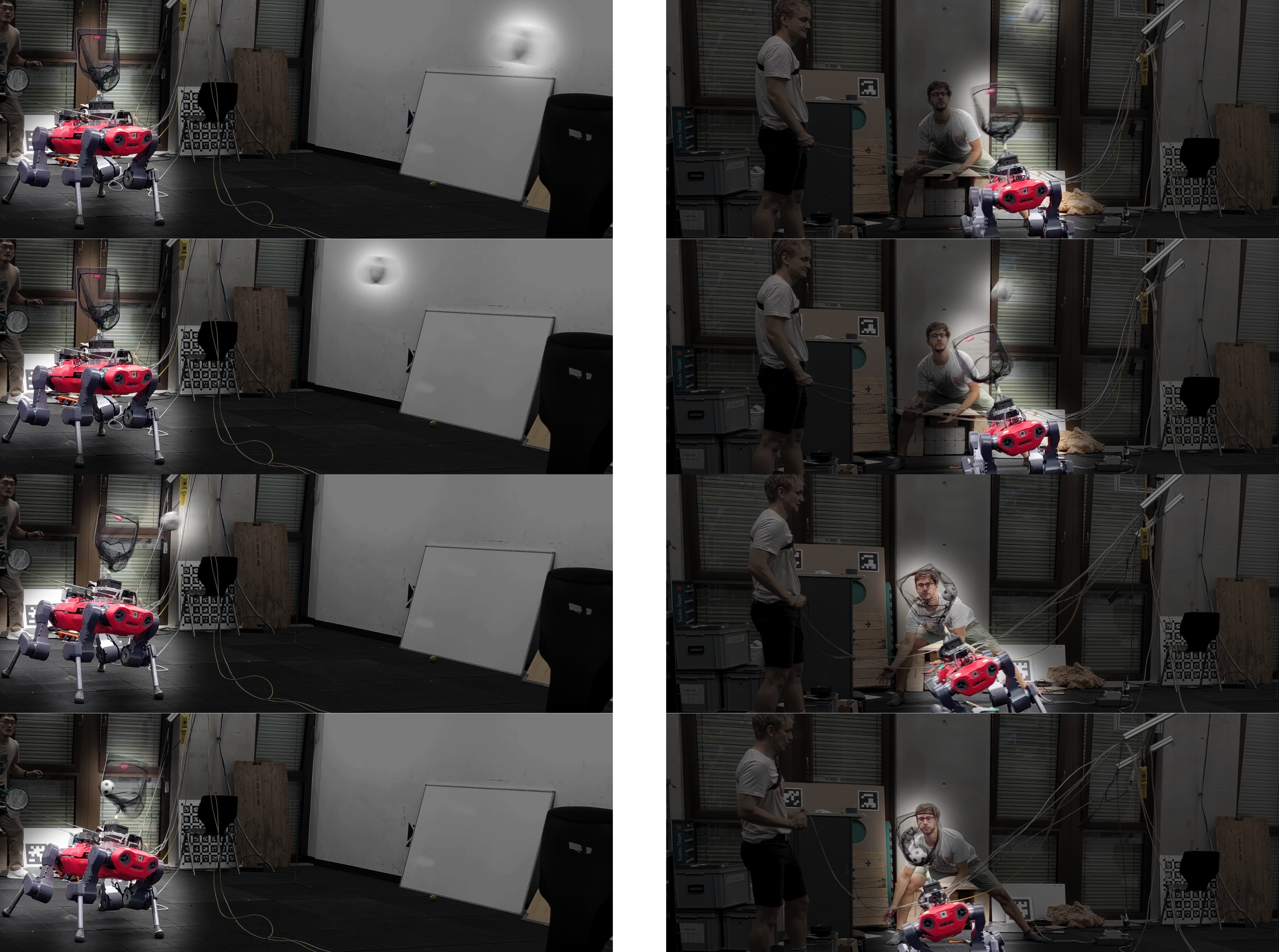
Results We find from Tab. II that our vision algorithm only degrades at speeds m/s and deviations from the net position of m. At 15 m/s and 0.6 m deviation, we still capture 50.25% of the impact points within a reasonable accuracy for catching. The degradation can be explained by two factors: as speed increases, fewer samples are collected to fit a parabola, reducing its overall accuracy. Similarly, throwing the ball further out, means that the ball quickly leaves the FoV, resulting in fewer observations. In Tab. I we find that catching success rate remains above 80% reaching a maximum at m/s. Two examples of successful catching maneuvers can be found in Fig. 5. We found that too high speeds cause vision to fail more often due to too few samples being recorded. Additionally, the robot cannot react fast enough to catch the objects. Conversely, at too low speeds, our vision algorithm can correctly identify where the robot should go, but the low speeds cause higher variability in the range of the trajectory and the impact angle at which the ball trajectory reaches the robot becomes steeper. If objects arrive at steep impact angles, the effective area with which the robot can catch the object is reduced. The impact angle is not directly observed by our policy, which reduces its robustness to this factor.
| Object Speed [m/s] | |||
| <8.0 | <10.0 | <12.0 | <15.0 |
| Distance from Net Position [m] | Object Speed [m/s] | |
|---|---|---|
| <9 | <15 | |
| <0.4 | ||
| <0.6 | ||
VI Discussion
The current work demonstrates agile catching of high-speed objects between m/s with a quadruped robot using an event camera for estimating the ballistic trajectories of the flying objects. Being the first example of catching with a quadruped robot using onboard sensing, our pipeline demonstrates agile catching skills and catches balls coming at a m deviation from the current center of the landing net. Importantly, as shown in II, the onboard event-based ball-tracking pipeline performs reliably on a larger range of m, making sure that the estimations provided to the rather dynamic motion policy will always be adequate. While this approach was enough for the first working demo of quadruped catching with onboard sensing, improvements could be made to improve the robot’s "range" to the side by for example using a higher FoV camera. Since our method is monocular, it requires knowledge of the object size. However, this requirement could be easily lifted by using a stereo setup, which would also reduce depth uncertainty making us less reliant on filtering. Also, the current control strategy was simply reaching the target position as quickly as possible. By taking into account the ball movement, sensor property and detection pipeline during the training, the trained policy could further improve its capability. Finally, to eliminate failure cases due to steep impact trajectories, which reduce the effective net area, we may consider augmenting our policy input by the velocity vector at the impact point.
VII Conclusion
On the quest toward animal-like agility and robustness, current quadruped robots have reached a high degree of versatility through the use of both proprioceptive and exteroceptive sensors. However, commonly used sensors such as RGB cameras or LiDARs currently suffer from major limitations due to the bandwidth-latency trade-off, meaning that both low-latency and low-bandwidth cannot be achieved with current systems. In this work, we break this cycle by outfitting a quadrupedal robot with an event camera, which does not have this tradeoff. We design a method that combines a high-speed visual frontend with a learning-based planner to perform the complex task of agile ball-catching. Thanks to the low latency of the event camera, as well as the robustness of the planner we reach an 83% success rate while catching objects thrown at up to 15 m/s.
References
- [1] T. Miki, J. Lee, J. Hwangbo, L. Wellhausen, V. Koltun, and M. Hutter, “Learning robust perceptive locomotion for quadrupedal robots in the wild,” Science Robotics, vol. 7, no. 62, p. eabk2822, 2022.
- [2] J. Lee, J. Hwangbo, and M. Hutter, “Robust recovery controller for a quadrupedal robot using deep reinforcement learning,” Jan. 2019.
- [3] K. Su and S. Shen, “Catching a flying ball with a vision-based quadrotor,” in International Symposium on Experimental Robotics. Springer, 2016, pp. 550–562.
- [4] D. Falanga, K. Kleber, and D. Scaramuzza, “Dynamic obstacle avoidance for quadrotors with event cameras,” Science Robotics, vol. 5, no. 40, p. eaaz9712, Mar. 2020.
- [5] N. J. Sanket, C. M. Parameshwara, C. D. Singh, A. V. Kuruttukulam, C. Fermüller, D. Scaramuzza, and Y. Aloimonos, “Evdodgenet: Deep dynamic obstacle dodging with event cameras,” in IEEE Int. Conf. Robot. Autom. (ICRA). IEEE, 2020, pp. 10 651–10 657.
- [6] D. Falanga, S. Kim, and D. Scaramuzza, “How fast is too fast? the role of perception latency in high-speed sense and avoid,” IEEE Robotics and Automation Letters, vol. 4, no. 2, pp. 1884–1891, 2019.
- [7] S. Kim, A. Shukla, and A. Billard, “Catching objects in flight,” IEEE Trans. Robot., vol. 30, no. 5, pp. 1049–1065, 2014.
- [8] P. Bouffard, A. Aswani, and C. Tomlin, “Learning-based model predictive control on a quadrotor: Onboard implementation and experimental results,” in IEEE Int. Conf. Robot. Autom. (ICRA). IEEE, 2012, pp. 279–284.
- [9] Z. Wang, F. C. Ojeda, A. Bisulco, D. Lee, C. J. Taylor, K. Daniilidis, M. A. Hsieh, D. D. Lee, and V. Isler, “Ev-catcher: High-speed object catching using low-latency event-based neural networks,” IEEE Robot. Autom. Lett., vol. 7, no. 4, pp. 8737–8744, 2022.
- [10] P. D. Neuhaus, J. E. Pratt, and M. J. Johnson, “Comprehensive summary of the institute for human and machine cognition’s experience with LittleDog,” The International Journal of Robotics Research, vol. 30, no. 2, pp. 216–235, 2011.
- [11] F. Jenelten, T. Miki, A. E. Vijayan, M. Bjelonic, and M. Hutter, “Perceptive locomotion in rough terrain–online foothold optimization,” IEEE Robotics and Automation Letters, vol. 5, no. 4, pp. 5370–5376, 2020.
- [12] R. Grandia, F. Jenelten, S. Yang, F. Farshidian, and M. Hutter, “Perceptive locomotion through nonlinear model predictive control,” Aug. 2022.
- [13] J. Hwangbo, J. Lee, A. Dosovitskiy, D. Bellicoso, V. Tsounis, V. Koltun, and M. Hutter, “Learning agile and dynamic motor skills for legged robots,” Sci Robot, vol. 4, no. 26, Jan. 2019.
- [14] J. Lee, J. Hwangbo, L. Wellhausen, V. Koltun, and M. Hutter, “Learning quadrupedal locomotion over challenging terrain,” Science Robotics, vol. 5, no. 47, 2020.
- [15] X. B. Peng, E. Coumans, T. Zhang, T.-W. Lee, J. Tan, and S. Levine, “Learning agile robotic locomotion skills by imitating animals,” Robotics: Science and Systems, 2020.
- [16] J. Siekmann, K. Green, J. Warila, A. Fern, and J. Hurst, “Blind bipedal stair traversal via sim-to-real reinforcement learning,” arXiv preprint arXiv:2105.08328, 2021.
- [17] D. Kim, D. Carballo, J. Di Carlo, B. Katz, G. Bledt, B. Lim, and S. Kim, “Vision aided dynamic exploration of unstructured terrain with a small-scale quadruped robot,” in 2020 IEEE International Conference on Robotics and Automation (ICRA). IEEE, 2020, pp. 2464–2470.
- [18] P. Fankhauser, M. Bjelonic, C. D. Bellicoso, T. Miki, and M. Hutter, “Robust rough-terrain locomotion with a quadrupedal robot,” in 2018 IEEE International Conference on Robotics and Automation (ICRA). IEEE, 2018, pp. 5761–5768.
- [19] T. Miki, L. Wellhausen, R. Grandia, F. Jenelten, T. Homberger, and M. Hutter, “Elevation mapping for locomotion and navigation using GPU,” in IEEE/RSJ Int. Conf. Intell. Robot. Syst. (IROS), 2022.
- [20] W. Yu, D. Jain, A. Escontrela, A. Iscen, P. Xu, E. Coumans, S. Ha, J. Tan, and T. Zhang, “Visual-locomotion: Learning to walk on complex terrains with vision,” in Proceedings of the 5th Conference on Robot Learning, ser. Proceedings of Machine Learning Research, A. Faust, D. Hsu, and G. Neumann, Eds., vol. 164. PMLR, 08–11 Nov 2022, pp. 1291–1302. [Online]. Available: https://proceedings.mlr.press/v164/yu22a.html
- [21] R. Yang, M. Zhang, N. Hansen, H. Xu, and X. Wang, “Learning vision-guided quadrupedal locomotion end-to-end with cross-modal transformers,” in International Conference on Learning Representations, 2022. [Online]. Available: https://openreview.net/forum?id=nhnJ3oo6AB
- [22] X. Huang, Z. Li, Y. Xiang, Y. Ni, Y. Chi, Y. Li, L. Yang, X. B. Peng, and K. Sreenath, “Creating a dynamic quadrupedal robotic goalkeeper with reinforcement learning,” arXiv preprint arXiv:2210.04435, 2022.
- [23] M. Ester, H.-P. Kriegel, J. Sander, and X. Xu, “A density-based algorithm for discovering clusters in large spatial databases with noise,” in KDD, 1996.
- [24] J. Schulman, F. Wolski, P. Dhariwal, A. Radford, and O. Klimov, “Proximal policy optimization algorithms,” arXiv preprint arXiv:1707.06347, 2017.
- [25] M. Hutter, C. Gehring, D. Jud, A. Lauber, C. D. Bellicoso, V. Tsounis, J. Hwangbo, K. Bodie, P. Fankhauser, M. Bloesch, et al., “Anymal-a highly mobile and dynamic quadrupedal robot,” in 2016 IEEE/RSJ international conference on intelligent robots and systems (IROS). IEEE, 2016, pp. 38–44.
- [26] V. Makoviychuk, L. Wawrzyniak, Y. Guo, M. Lu, K. Storey, M. Macklin, D. Hoeller, N. Rudin, A. Allshire, A. Handa, and Gavriel State, “Isaac gym: High performance GPU-Based physics simulation for robot learning,” Aug. 2021.
- [27] N. Rudin, D. Hoeller, P. Reist, and M. Hutter, “Learning to walk in minutes using massively parallel deep reinforcement learning,” in Conf. on Robotics Learning (CoRL). PMLR, 2022, pp. 91–100.
- [28] P. Lichtsteiner, C. Posch, and T. Delbruck, “A 128128 120 dB 15 s latency asynchronous temporal contrast vision sensor,” IEEE J. Solid-State Circuits, vol. 43, no. 2, pp. 566–576, 2008.