Contrastive Hierarchical Clustering

Abstract

Deep clustering has been dominated by flat models, which split a dataset into a predefined number of groups. Although recent methods achieve an extremely high similarity with the ground truth on popular benchmarks, the information contained in the flat partition is limited. In this paper, we introduce CoHiClust, a Contrastive Hierarchical Clustering model based on deep neural networks, which can be applied to typical image data. By employing a self-supervised learning approach, CoHiClust distills the base network into a binary tree without access to any labeled data. The hierarchical clustering structure can be used to analyze the relationship between clusters, as well as to measure the similarity between data points. Experiments demonstrate that CoHiClust generates a reasonable structure of clusters, which is consistent with our intuition and image semantics. Moreover, it obtains superior clustering accuracy on most of the image datasets compared to the state-of-the-art flat clustering models. Our implementation is available at https://github.com/MichalZnalezniak/Contrastive-Hierarchical-Clustering.

1 Introduction

Clustering, a fundamental branch of unsupervised learning, is often one of the first steps in data analysis, which finds applications in anomaly detection [2], personalized recommendations [45] or bioinformatics [22]. Since it does not use any information about class labels, representation learning becomes an integral part of deep clustering methods. Initial approaches use representations taken from pre-trained models [13, 30] or employ autoencoders in joint training of the representation and the clustering model [14, 26]. Recent models designed to image data frequently follow the self-supervised learning principle, where the representation is trained on pairs of similar images generated automatically by data augmentations [23, 9]. Since augmentations used for image data are class-invariant, the latter techniques of ten obtain a very high similarity to the ground truth classes. However, we should be careful when comparing clustering techniques only by inspecting their accuracy with ground truth classes because the primary goal of clustering is to deliver information about data and not to perform classification.

Figure 1: A hierarchy generated by CoHiClust for ImageNet-10. As can be seen, CoHiClust reliably reflected the ground-truth classes in leaf nodes. In addition to information delivered by flat partition, in hierarchical models neighbor leaves contain images sharing similar characteristic. It is evident that images with soccer ball are similar to pictures with oranges because of their shapes. Dogs are more similar to leopards than to penguins, which is reflected in the constructed hierarchy. The same hold when analyzing the leafs representing cars, trucks and ships. Looking at the first hierarchy level, we observe a distinction on the right sub-tree representing machines and left-sub-tree dominated by animals. Moreover, balls and oranges are separated from the animal branch.

Most of the works in the area of deep clustering focus on producing flat partitions with a predefined number of groups. Although hierarchical clustering has gained considerable attention in classical machine learning and has been frequently applied in real-life problems [46, 32], its role has been drastically marginalized in the era of deep learning. In the case of hierarchical clustering, the exact number of clusters does not have to be specified because we can inspect the partition at various tree levels. Moreover, we can analyze the clusters’ relationships, e.g. by finding superclusters or measuring the distance between groups in the hierarchy. These advantages make hierarchical clustering an excellent tool for analyzing complex data. However, to take full advantage of hierarchical clustering, it is necessary to create an appropriate image representation, which is possible due to the use of deep neural networks. To our knowledge, DeepECT [26, 27] is the only hierarchical clustering model trained jointly with the neural network. However, this method has not been examined for larger datasets of color images.

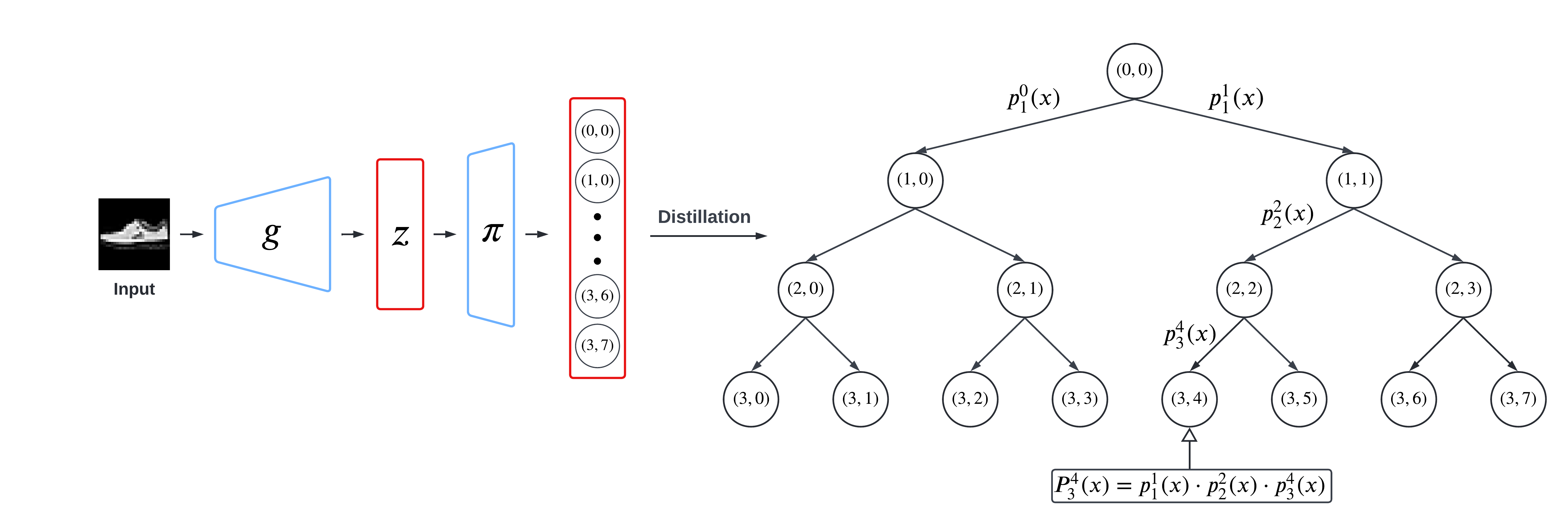
To fill this gap, we introduce CoHiClust (Contrastive Hierarchical Clustering), which creates a cluster hierarchy and works well on typical color image databases. CoHiClust uses a neural network to generate a high-level representation of data, which is then distilled into the tree hierarchy by applying the projection head, see Figure 2. The whole framework is trained jointly in an end-to-end manner without labels using our novel contrastive loss and data augmentations generated automatically following the self-supervised learning principle.

The constructed hierarchy uses the structure of a binary tree, where the sequence of decisions made by the internal nodes determines the final assignment to the clusters (leaf nodes). In consequence, similar examples are processed longer by the same path than dissimilar ones. By inspecting the number of edges needed to connect two clusters (leaves), we obtain a natural similarity measure between data points. By applying a pruning strategy, which removes the least informative leaf nodes, we can restrict the hierarchy to a given number of leaves and fine-tune the whole hierarchy.

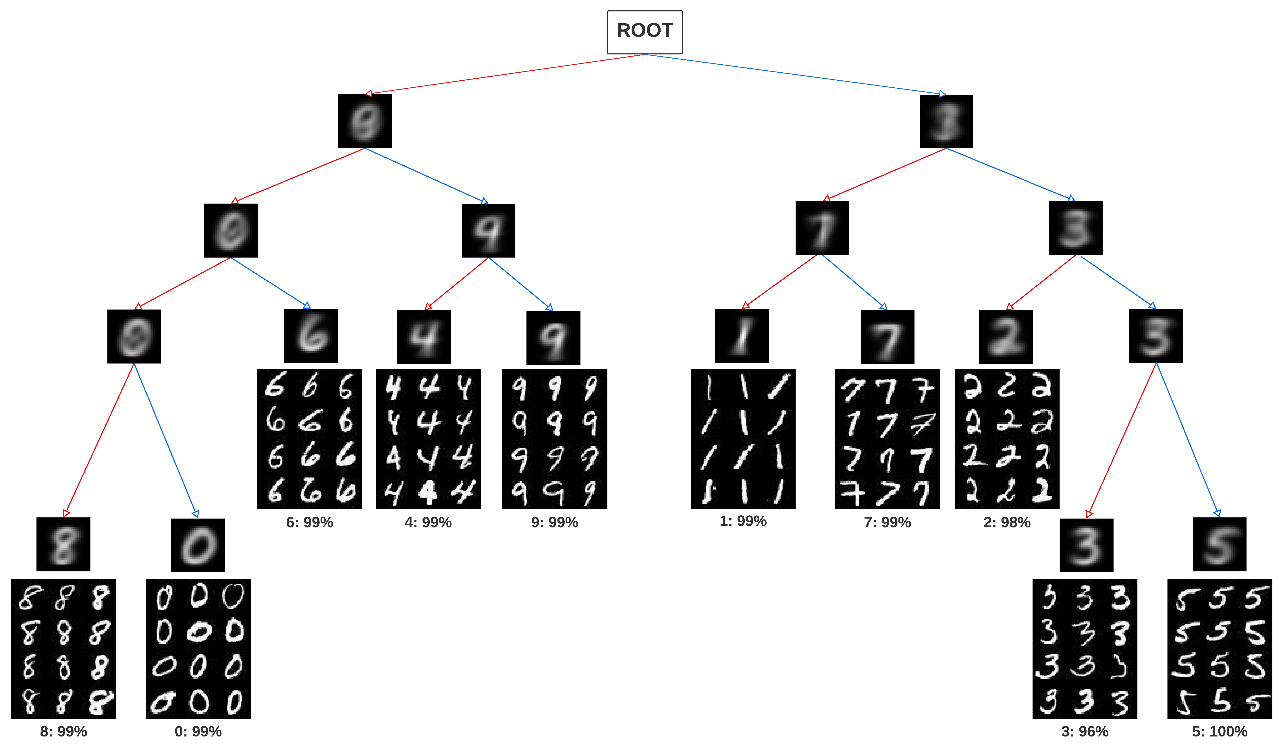
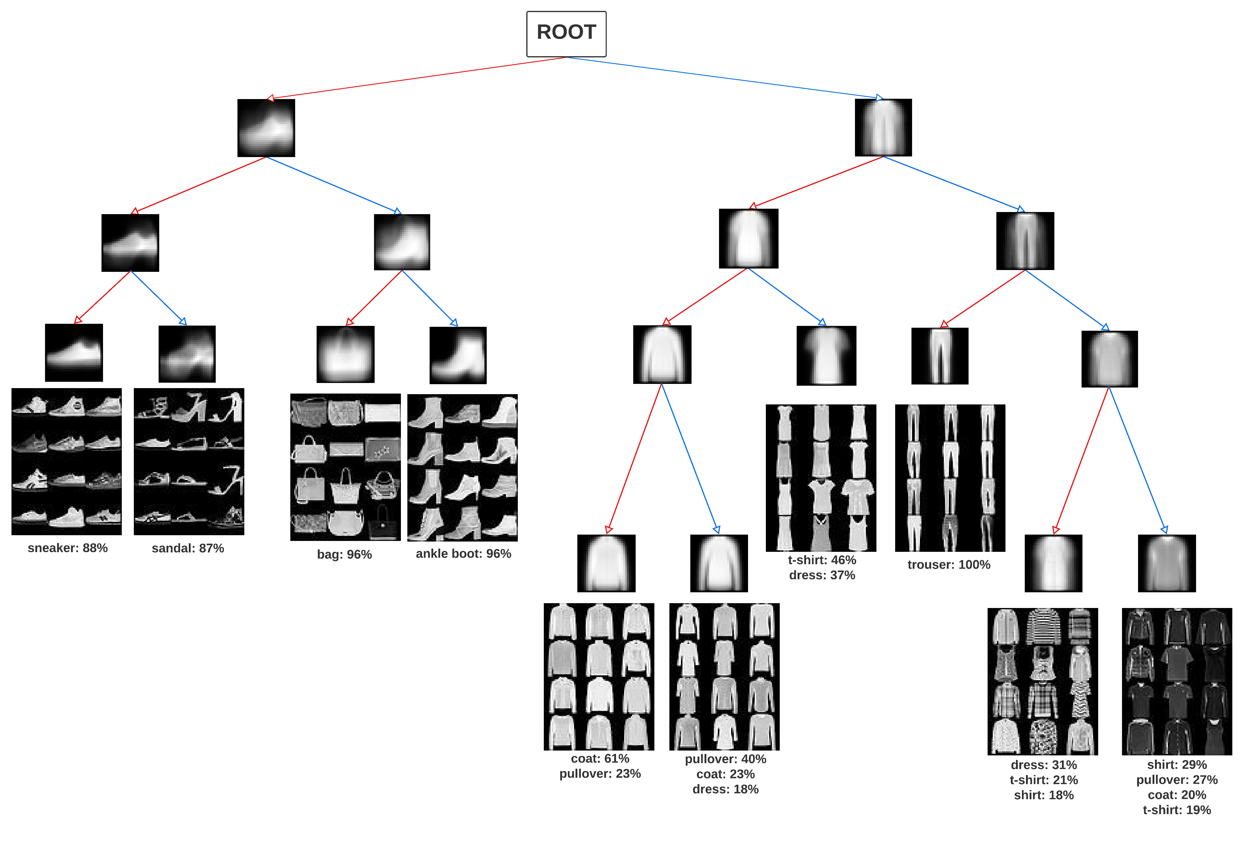
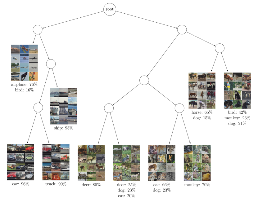
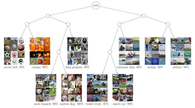
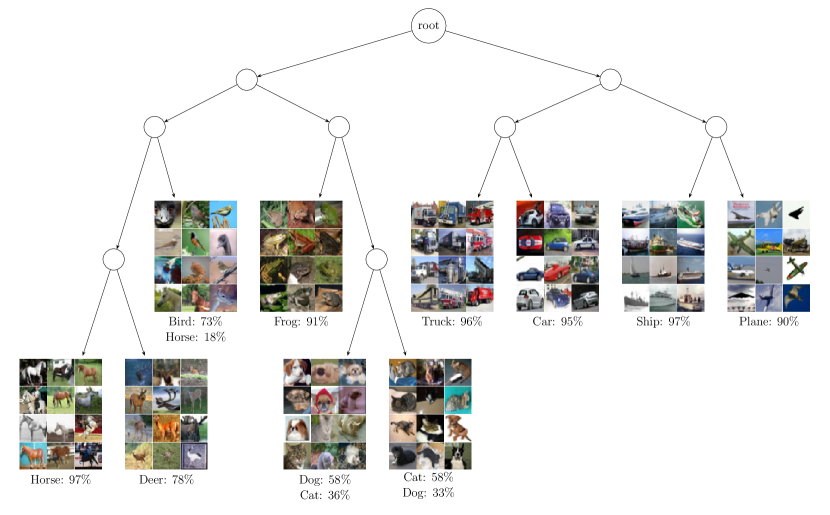
The proposed model has been examined on various image datasets and compared with hierarchical and flat clustering baselines. By analyzing the constructed hierarchies, we show that CoHiClust generates a structure of clusters that is consistent with our intuition and image semantics, see Figures 1 and 3 for illustration and discussion. Our analysis is supported by a quantitative study, which shows that CoHiClust outperforms the current clustering models on 5 out of 7 image datasets, see Tables 1 and 6.

Our main contributions are summarized as follows:

• We introduce a hierarchical clustering model CoHiClust, which converts the base neural network into a binary tree. The model is trained effectively without supervision using our novel hierarchical contrastive loss applied to self-generated data augmentations.

• We conducted an extensive experimental study, which confirms that CoHiClust is very competitive with current state-of-the-art flat clustering models. Moreover, we show that it builds hierarchies based on well-defined and intuitive patterns retrieved from the data.

• Since CoHiClust is the first deep hierarchical clustering model applied to color image datasets, we provide a benchmark, which can be used to compare hierarchical clustering methods.

2 Related Work

In this section, we briefly introduce some recent developments on three related topics: contrastive learning, deep clustering, and hierarchical methods.

Contrastive Learning

The basic idea of contrastive learning is to learn a feature space in which similar pairs stay close to each other, while dissimilar ones are far apart [8]. In recent works, it was observed that in selected domains, such as computer vision, positive (similar) pairs can be generated automatically using adversarial perturbations [28] or data augmentation [16], giving rise to a new field called self-supervised learning [7]. Fine-tuning a simple classifier on self-supervised representation allows for obtaining the accuracy comparable to a fully supervised setting. SimCLR [16] applies NT-Xent loss to maximize the agreement between differently augmented views of the same sample. Barlow Twins [41] learns to make the cross-correlation matrix between two distorted versions of the same samples close to the identity. BYOL [12] claims to achieve new state-of-the-art results without using negative samples. Other works use memory banks to reduce the cost of computing the embeddings of negative samples in every batch [37, 16].

Deep clustering

A primary focus in deep embedded clustering has merely been on flat clustering objectives with the actual number of clusters known a priori. DEC [38] is one of the first works, which combines the auto-encoder loss with a clustering objective to jointly learn the representation and perform clustering. This idea was further explored with some improvements in IDEC [14], JULE [39] and DCEC [15]. IMSAT [17] and IIC [19] use perturbations to generate pairs of similar examples and apply information-theoretic objectives for training. PICA [18] maximizes the global partition confidence of the clustering solution to find the most semantically plausible data separation. Following progress in self-supervised learning, CC [23] and DCSC [44] perform contrastive learning by generating pairs of positive and negative instances through data augmentations.

Hierarchical methods

Hierarchical clustering algorithms are a well-established area within classical data mining [29], but have rarely been studied in deep learning. DeepECT [26, 27] is the only method that jointly learns deep representation using autoencoder architecture and performs hierarchical clustering in a top-down manner. Unfortunately, no comparative study has been conducted on large image data. The experimental study of objective-based hierarchical clustering methods performed on the embedding vectors of pre-trained deep learning models is presented in [30]. In the case of classification, there is a growing interest in deep hierarchical methods, which in our opinion should also be reflected in the area of unsupervised learning. SDT [10] is one of the first models that distills the base neural networks into a soft decision tree. More advanced methods automatically generate deep networks with a tree structure in a multistep or end-to-end manner [33, 1, 35].

3 CoHiClust model

The proposed CoHiClust builds a hierarchy of clusters based on the output of the base neural network. There are three key components of CoHiClust:

• The base neural network that generates the representation used by the tree.

• The tree model, which assigns data points to clusters by a sequence of decisions.

• The regularized contrastive loss, which allows for training the whole framework.

We discuss the above components in detail in the following parts.

3.1 Tree hierarchy

We use a soft binary decision tree to create a hierarchical structure, where leaves play the role of clusters (similar to [10]). In contrast to hard decision trees, every internal node defines the probability of taking a left/right branch. The final assignment of the input examples to clusters involves partial decisions made by the internal nodes. Aggregating these decisions induces the posterior probability over leaves.

Let us consider a complete binary tree with $T$ levels, where the root is located at the level $0$ and the leaves are represented at the level $T$. This gives us $2^{t}$ nodes at the level $t$ denoted by tuples $(t,i)$, for $i=0,1,\ldots,2^{t}-1$, see Figure 2. The path from root to node $(t,i)$ is given by the sequence of binary decisions $y=(y_{1},\ldots,y_{t})\in\{0,1\}^{t}$ made by the internal nodes, where $y_{s}=0$ ($y_{s}=1$) means that we take the left (right) branch that is at the node at the level $s$. Observe that we can retrieve the index $j$ of the node at the level $s$ from $y$ by taking ${j=b_{s}(y)=\sum_{m=1}^{s}y_{m}2^{s-m}}$. In other words, the first $s$ bits of $y$ are a binary representation of the number $j$.

We consider the path induced by the sequence of decisions $y=(y_{1},\ldots,y_{t})\in\{0,1\}^{t}$, which goes from the root to the node $(t,i)$, where $i=b_{t}(y)$. We want to calculate the probability $P_{t}^{i}(x)$ that the input example $x\in\mathbb{R}^{D}$ reaches node $(t,i)$. If $p_{s}^{b_{s}(y)}(x)$ is the probability of going from the parent node $(s-1,b_{s-1}(y))$ to its descendant $(s,b_{s}(y))$, then

$$P_{t}^{i}(x)=p_{1}^{b_{1}(y)}(x)\cdot p_{2}^{b_{2}(y)}(x)\cdot\ldots p_{t}^{b_{t}(y)}(x).$$

Observe that $P_{t}(x)=[P_{t}^{0}(x),P_{t}^{1}(x),\ldots,P_{t}^{2^{t}-1}(x)]$ defines a proper probability distribution, i.e. ${\sum_{j=0}^{2^{t}-1}P_{t}^{j}(x)=1}$. As a consequence, the probability distribution on the clusters (leaves) is equal to $P_{T}(x)$, see Figure 2.

Figure 2: Illustration of CoHiClust. The output neurons of the projection head $\pi$ (appended to the base network $g$) model decisions made by the internal tree nodes. The final assignment of the input example to the cluster (leaf node) is performed by aggregating edge probabilities located on the path from the root to this leaf.

3.2 Tree generation

To generate our tree model, we need to parameterize the probabilities $p_{t}^{i}(x)$ of taking the left/right branch in every internal node. To this end, we employ a neural network $g:\mathbb{R}^{D}\to\mathbb{R}^{N}$ with an additional projection head $\pi:\mathbb{R}^{N}\to\mathbb{R}^{K}$, where $K=2^{T}-1$ and $T$ is the height of the tree. The number $K$ of output neurons equals the number of internal tree nodes.

The neural network $g$ is responsible for extracting high-level information from the data. It can be instantiated by a typical architecture, such as ResNet, and is used to generate embeddings $z=g(x)$ of the input data.

The projection head $\pi$ operates on the embeddings $z$ and parameterizes the decisions made by the internal tree nodes. In our case, $\pi$ is a single layer network with the output dimension equal to the number of internal nodes. To model binary decisions of internal nodes, we apply the sigmoid function $\sigma$. Consequently, the projection head is given by $\pi(z)=[\sigma(w_{1}^{T}z+b_{1}),\ldots,\sigma(w_{K}^{T}z+b_{K})]$, where $w_{n}\in\mathbb{R}^{N}$ and $b_{n}\in\mathbb{R}$ are trainable parameters of $\pi$. By interpreting the output neurons of $\pi$ as the internal nodes of the decision tree, we obtain the probabilities of the left edges in the nodes:

$$p_{t+1}^{2i}(x)=\sigma(w_{n}^{T}z+b_{n})\text{ , for }n=2^{t}+i.$$

Note that $p_{t+1}^{2i-1}(x)=1-p_{t+1}^{2i}(x)$ always corresponds to the probability of the right edge.

3.3 Contrastive hierarchical loss

To train CoHiClust, we introduce the hierarchical contrastive loss function designed for trees. Our idea is based on maximizing the likelihood that similar data points will follow the same path. The more similar data points, the longer they should be routed through the same nodes. Since we work in an unsupervised setting, we use a self-supervised approach and generate similar images using data augmentations.

Let us consider two data points $x_{1},x_{2}$ and their posterior probabilities $P_{t}(x_{1}),P_{t}(x_{2})$ at the level $t$. The probability that $x_{1}$ and $x_{2}$ reach the same node at this level is given by the scalar product $P_{t}(x_{1})\cdot P_{t}(x_{2})=\sum_{i=0}^{2^{t}-1}P_{t}^{i}(x_{1})P_{t}^{i}(x_{2})$. This term is maximal if both probabilities are identical one-hot vectors. In a training phase, we do not want to force hard splits in the nodes (binary probabilities), because in this way the model quickly finds a local minimum by assigning data points to fixed leaves with high confidence. Instead of sticking to hard assignments in a few training epochs, we want to let the model explore possible solutions. To this end, we take the square root before applying the scalar product, which corresponds to the Bhattacharyya coefficient [4]:

$$s_{t}(x_{1},x_{2})=\sqrt{P_{t}(x_{1})\cdot P_{t}(x_{2})}=\sum_{i=0}^{2^{t}-1}\sqrt{P_{t}^{i}(x_{1})P_{t}^{i}(x_{2})}.$$ (1)

Observe that $s_{t}(x_{1},x_{2})=1$, if only $P_{t}(x_{1})=P_{t}(x_{2})$ (probabilities do not have to binarize), which leads to the exploration of possible paths. By aggregating the similarity scores over all tree levels, we arrive at our final similarity function $s(x_{1},x_{2})=\sum_{t=0}^{T-1}s_{t}(x_{1},x_{2})$.

In a training phase, we take a minibatch $\{x_{j}\}_{j=1}^{N}$ of $N$ examples and generate its augmented view $\{\tilde{x}_{j}\}_{j=1}^{N}$. Every pair $(x_{j},\tilde{x}_{j})$ is considered positive, which means that we will maximize their similarity score. As a consequence, we encourage the model to assign them to the same leaf node. To avoid degenerate solutions, where all points end up in the same leaf, we treat all other pairs as negative and minimize their similarity scores. Finally, the proposed hierarchical contrastive loss is given by:

$$\mathrm{CoHiLoss}=\frac{1}{N(N-1)}\sum_{j=1}^{N}\sum_{i\neq j}s(x_{j},\tilde{x}_{i})-\frac{1}{N}\sum_{j=1}^{N}s(x_{j},\tilde{x}_{j}).$$

By minimizing the above loss, we maximize the likelihood that similar data points follow the same path (second term) and minimize the likelihood that dissimilar ones are grouped together.

3.4 Regularization

The final cluster assignments are induced by aggregating several binary decisions made by the internal tree nodes. In practice, the base neural network may not train all nodes and, in consequence, use only a few leaves for clustering. While selecting the number of clusters in flat clustering is desirable, here we would like to create a hierarchy, which is not restricted to a given number of leaves. To enable end-to-end training of the base neural network with an arbitrary number of leaves, we consider two regularization strategies.

The first regularization (dubbed $R_{1}$) explicitly encourages the model to use both left and right sub-trees equally [10]. We realize this postulate by minimizing the cross-entropy between the desired distribution $[0.5,0.5]$ and the actual distribution to choose the left or right path in a given node.

The second regularization (dubbed $R_{2}$) does not directly influence the routing in the tree, but focuses on improving the output representation of the base network $g$. For this purpose, we use a projection head $\phi:\mathbb{R}^{N}\to\mathbb{R}^{M}$, which transforms the embeddings $z=g(x)$ of the input data, and apply the NT-Xent loss [7] to $\tilde{z}=\phi(z)$. With the NT-Xent loss, we maximize the cosine similarity for all positive pairs and minimize the cosine similarity for all negative pairs. For simple datasets, such as MNIST or F-MNIST, $\phi$ is an identity function, while for more complex color images, it is a two-layer network.

Taking together the contrastive loss $\mathrm{CoHiLoss}$ with two regularization functions $R_{1}$ (for entropy) and $R_{2}$ (for NT-Xent), we arrive at our final loss:

$$\mathrm{Loss}= \mathrm{CoHiLoss}+\beta_{1}R_{1}+\beta_{2}R_{2},$$ (2)

where $\beta_{1},\beta_{2}$ are the hyperparameters that define the importance of the regularization terms $R_{1}$ and $R_{2}$, respectively. To generate a complete hierarchy (complete tree with assumed height), we set $\beta_{1}$ proportional to the depth of the tree $\beta_{1}=2^{-T}$ [10] and $\beta_{2}=1$ [24].

3.5 Training

CoHiClust can be trained end-to-end by minimizing (2). We verified that training is even more effective when we introduce a pre-training phase of the base neural network. To this end, we perform self-supervised representation learning of the base network $g$ using $R_{2}$ regularization (it corresponds to the SimCLR model [7]). In Section 4.2, we show that pre-training allows us to reduce the number of training epochs and leads to a better overall performance of CoHiClust.

The proposed model builds a complete tree with $2^{T}$ leaves. Although such a structure is useful for analyzing the hierarchy of clusters, in some cases we are interested in creating a tree with the requested number of groups. For this purpose, we apply a pruning step that reduces the least significant leaf nodes. Namely, we reduce leaves with the lowest expected fraction of data points: $P_{T}^{i}=\frac{1}{|X|}\sum_{x\in X}P_{T}^{i}(x)$. Pruning is realized after a few first training epochs of CoHiClust (after the pre-training phase). We remove one leave per epoch. Next, CoHiClust is trained with the final number of leaves.

4 Experiments

Table 1: Comparison with flat clustering methods on datasets of color images.

Dataset	CIFAR-10			CIFAR-100			STL-10			ImageNet-10			ImageNet-Dogs
Metrics	NMI	ACC	ARI	NMI	ACC	ARI	NMI	ACC	ARI	NMI	ACC	ARI	NMI	ACC	ARI
K-means [25]	0.087	0.229	0.049	0.084	0.130	0.028	0.125	0.192	0.061	0.119	0.241	0.057	0.055	0.105	0.020
SC [43]	0.103	0.247	0.085	0.090	0.136	0.022	0.098	0.159	0.048	0.151	0.274	0.076	0.038	0.111	0.013
AC [11]	0.105	0.228	0.065	0.098	0.138	0.034	0.239	0.332	0.140	0.138	0.242	0.067	0.037	0.139	0.021
NMF [5]	0.081	0.190	0.034	0.079	0.118	0.026	0.096	0.180	0.046	0.132	0.230	0.065	0.044	0.118	0.016
AE [3]	0.239	0.314	0.169	0.100	0.165	0.048	0.250	0.303	0.161	0.210	0.317	0.152	0.104	0.185	0.073
DAE [34]	0.251	0.297	0.163	0.111	0.151	0.046	0.224	0.302	0.152	0.206	0.304	0.138	0.104	0.190	0.078
DCGAN [31]	0.265	0.315	0.176	0.120	0.151	0.045	0.210	0.298	0.139	0.225	0.346	0.157	0.121	0.174	0.078
DeCNN [42]	0.240	0.282	0.174	0.092	0.133	0.038	0.227	0.299	0.162	0.186	0.313	0.142	0.098	0.175	0.073
VAE [20]	0.245	0.291	0.167	0.108	0.152	0.040	0.200	0.282	0.146	0.193	0.334	0.168	0.107	0.179	0.079
JULE [39]	0.192	0.272	0.138	0.103	0.137	0.033	0.182	0.277	0.164	0.175	0.300	0.138	0.054	0.138	0.028
DEC [38]	0.257	0.301	0.161	0.136	0.185	0.050	0.276	0.359	0.186	0.282	0.381	0.203	0.122	0.195	0.079
DAC [6]	0.396	0.522	0.306	0.185	0.238	0.088	0.366	0.470	0.257	0.394	0.527	0.302	0.219	0.275	0.111
DCCM [36]	0.496	0.623	0.408	0.285	0.327	0.173	0.376	0.482	0.262	0.608	0.710	0.555	0.321	0.383	0.182
PICA [18]	0.591	0.696	0.512	0.310	0.337	0.171	0.611	0.713	0.531	0.802	0.870	0.761	0.352	0.352	0.201
CC [24]	0.705	0.790	0.637	0.431	0.429	0.266	0.764	0.850	0.726	0.859	0.893	0.822	0.445	0.429	0.274
CoHiClust	0.779	0.839	0.731	0.467	0.437	0.299	0.584	0.613	0.474	0.907	0.953	0.899	0.411	0.355	0.232

First, we evaluate our method on several datasets of color images of various resolutions and with a diverse number of classes. In addition to reporting similarity scores with ground-truth partitions, we analyze the constructed hierarchies, which in our opinion is equally important in practical use-cases. Next, we perform an ablation study and investigate the properties of CoHiClust. Finally, we compare CoHiClust with existing hierarchical methods. Details of the experimental settings and additional results are included in the Appendix.

4.1 Clustering color images

Benchmark

We perform the evaluation on typical bemchmark datasets: CIFAR-10, CIFAR-100, STL-10, ImageNet-Dogs, and ImageNet-10, see the Appendix for their summary. We process each data set at its original resolution. Since none of the previous hierarchical methods have been examined on these datasets, we use the benchmark that includes the flat clustering methods reported in [24]. According to previous works in contrastive clustering, CoHiClust uses ResNet architectures as a backbone network. To measure the similarity of the constructed partition with the ground truth, we apply three widely-used clustering metrics: normalized mutual information (NMI), clustering accuracy (ACC), and adjusted rand index (ARI). In the Appendix, we also show the DP (dendrogram purity) of the hierarchies generated by CoHiClust.

Figure 3: A tree hierarchy generated by CoHiClust for CIFAR-10. There is an evident distinction into animals (left branch) and machines (right branch). Moreover, all neighbor leaves represent visually similar classes (horses and deers, dogs and cats, trucks and cars, ships and planes). Images with frogs seem to be visually similar to cats and dogs, which leads to their placement in the neighbor leaves (however cats and dogs are connected by a stronger relationship). Interestingly, a small portion of images with horses’ heads are grouped together with birds because of their similar shapes. Although there is a slight mismatch between dogs and cats classes, the left leaf contains pets with bright fur photographed in front, while the right leaf includes animals with dark fur presented from the side, which coincides with our intuition.

The results presented in Table 1 show that CoHiClust outperforms the comparative methods in 3 out of 5 datasets. It gives extremely good results on CIFAR-10 and ImageNet-10, but is notably worse than CC on STL-10. We suspect that lower performance on STL-10 can be caused by inadequate choice of the backbone architecture to process images at resolution $96\times 96$. Nevertheless, one should keep in mind that CoHiClust is the only hierarchical method in this comparison, and constructing a clustering hierarchy, which resembles ground truth classes, is more challenging than directly generating a flat partition.

Figure 4: Distance matrices retrieved from the constructed hierarchies for ground truth classes of CIFAR-10 dataset, see text in the paper for the interpretation.

Analyzing clustering hierarchies

To better analyze the results returned by CoHiClust, we plot the constructed hierarchies. Figures 1 and 3 present and discuss the results obtained for ImageNet-10 and CIFAR-10, respectively (we refer the reader to the Appendix for more examples). In both cases, CoHiClust was able to accurately model ground-truth classes as leaf nodes. In addition to the information contained in a flat partition, CoHiClust allows us to find relations between clusters. In particular, we observe that similar classes are localized on neighboring nodes.

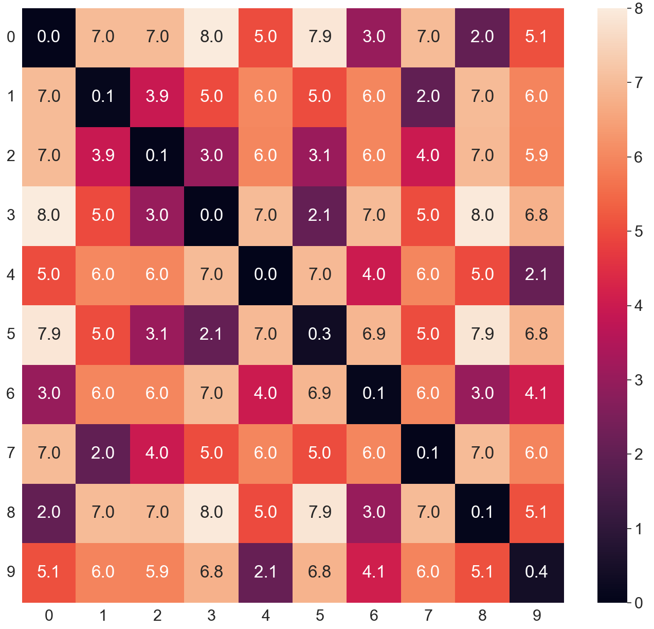
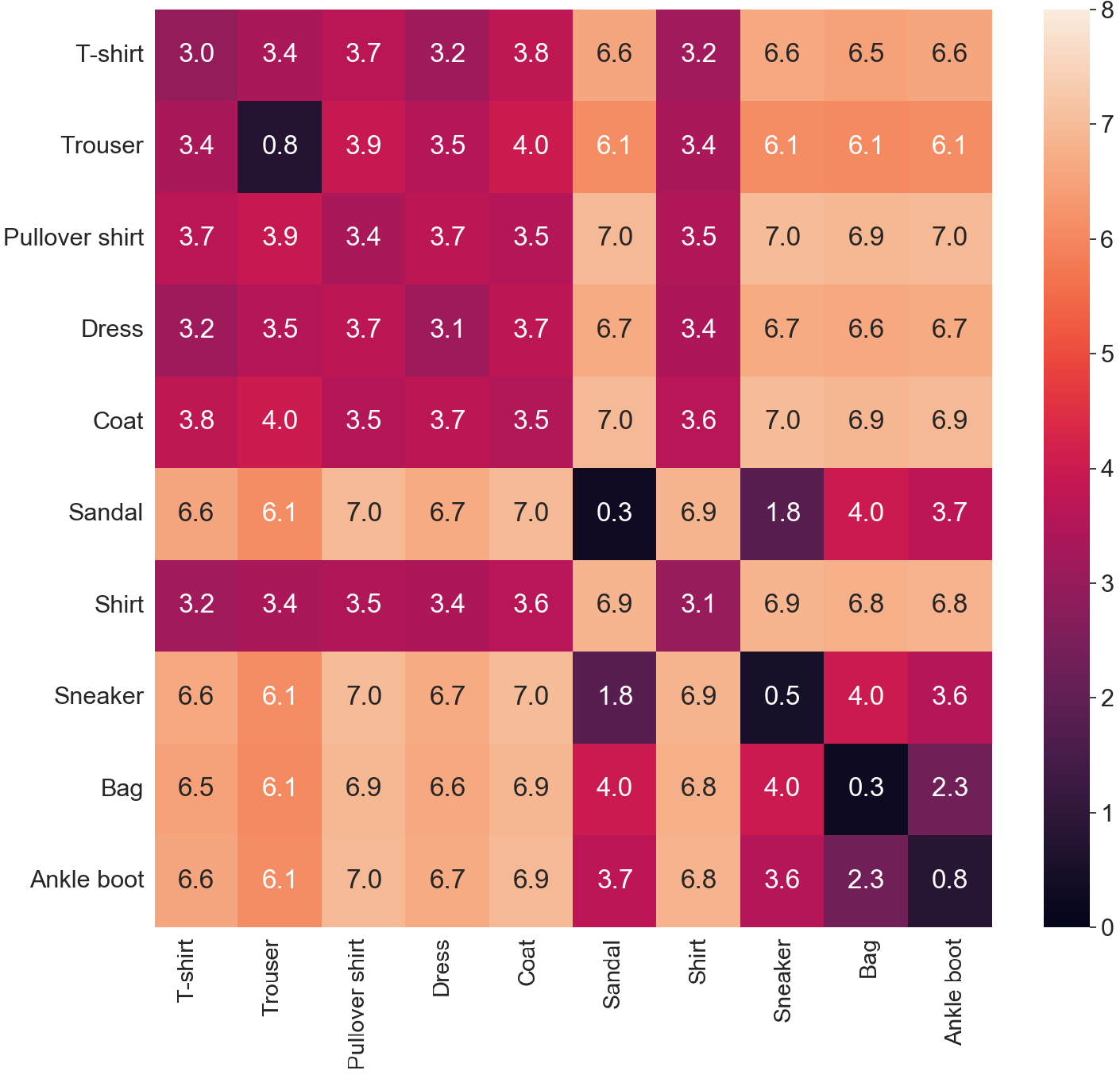
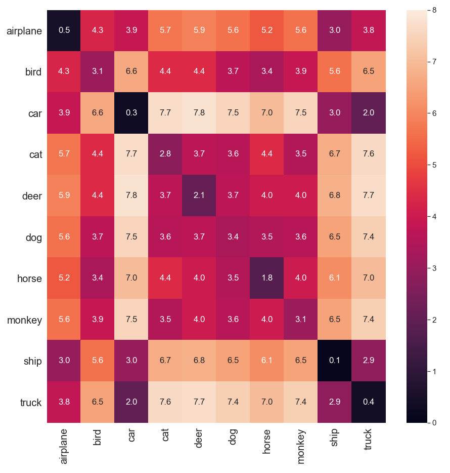
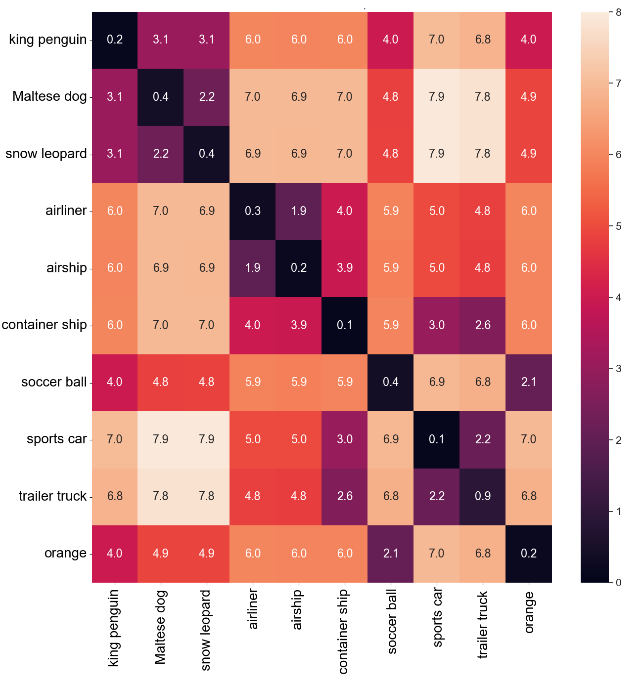
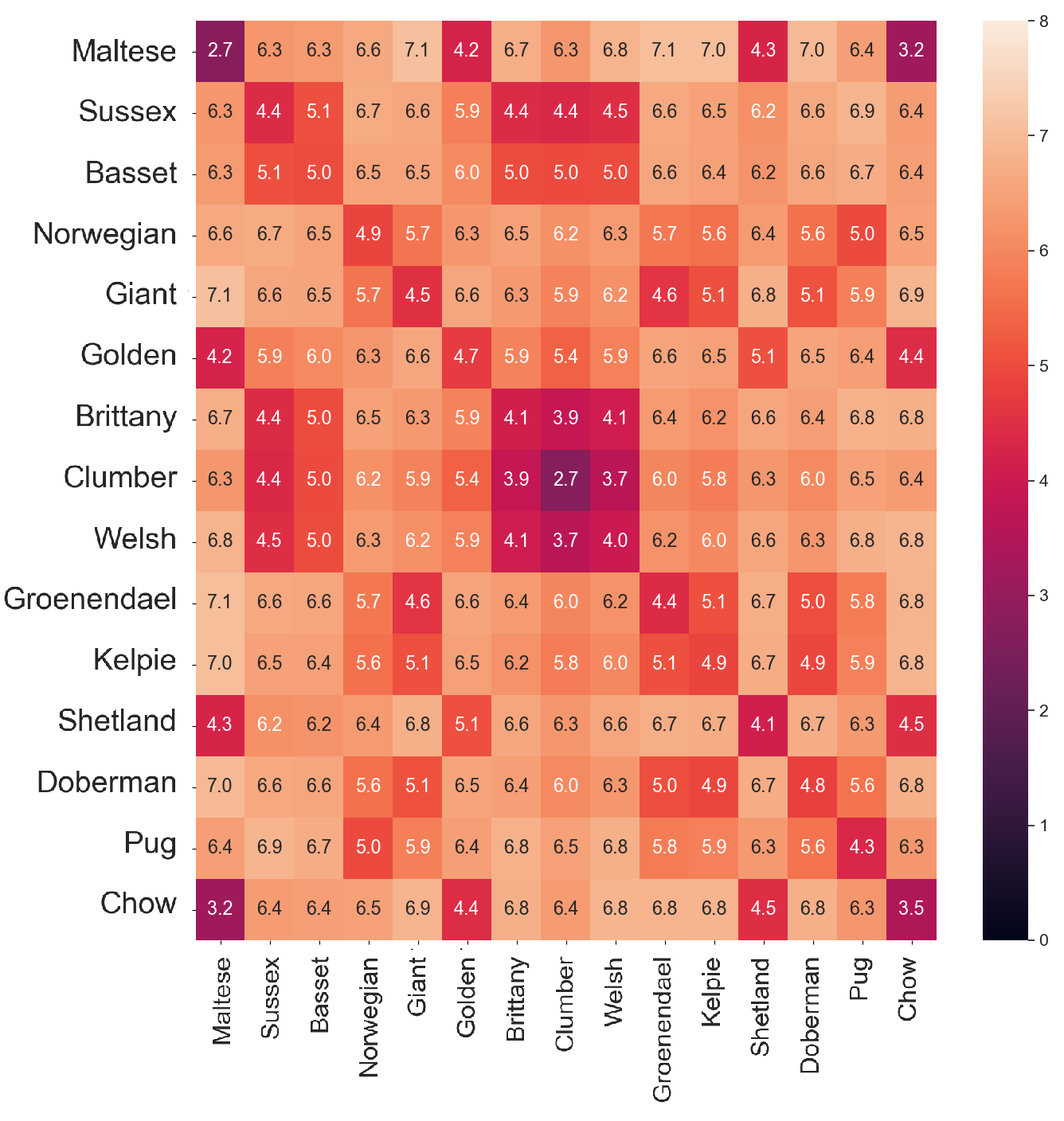
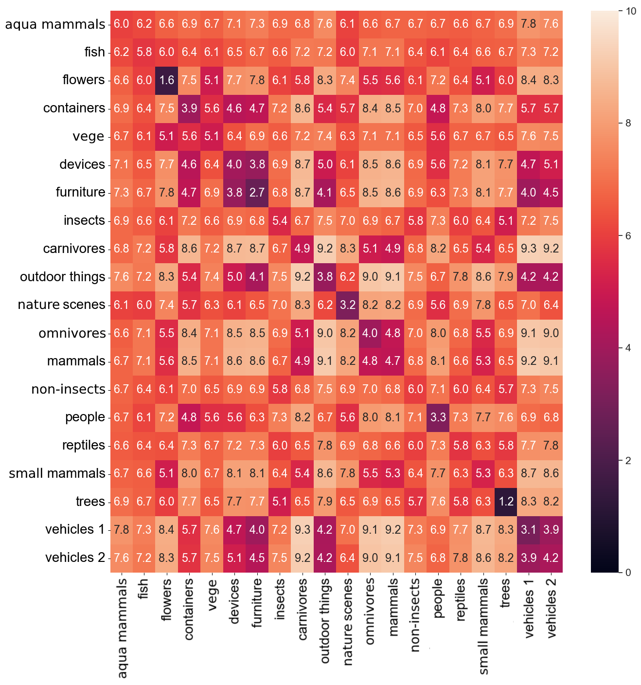
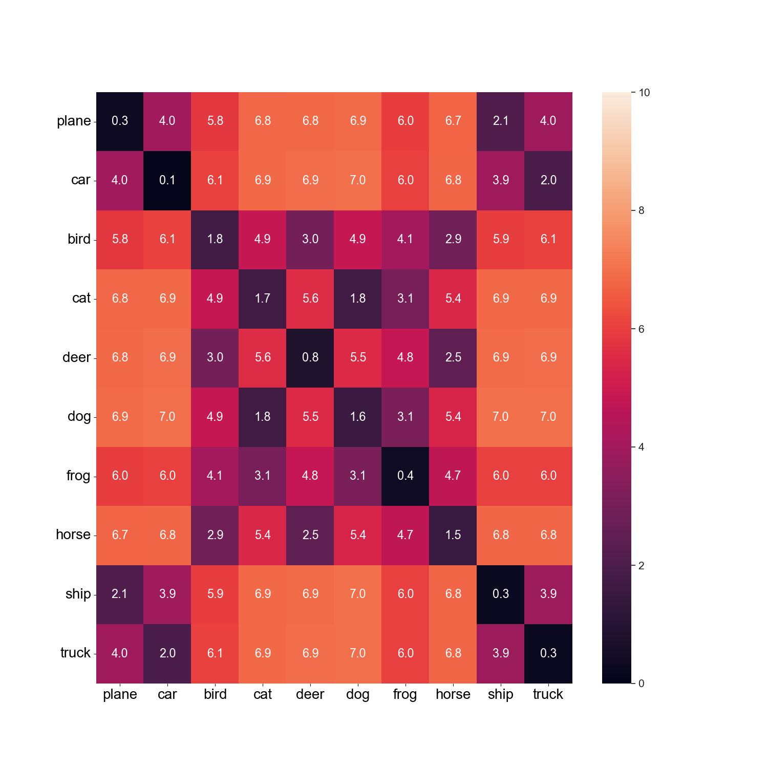
The hierarchy also allows us to define the distance $d(a,b)$ between two examples $a,b$ using the number of edges that connect them. We use the average of this score to calculate the similarity between the ground truth classes $A$ and $B$ as $d(A,B)=\frac{1}{Z}\sum_{a\in A}\sum_{b\in B}d(a,b)$, where $Z$ is the number of all pairs. The distance is small if examples from classes $A$ and $B$ are located in nearby leaf nodes (on average).

Analysis of the distance matrix in Figure 4 confirms that objects representing the same class have the strongest relationship in the hierarchy (the diagonal entries contain the smallest values in the matrix). We also see high similarities between classes representing dogs and cats (1.8 jumps), cars and trucks (2 jumps), etc. In general, the distance matrix supports our previous findings quantitatively.

4.2 Analysis of the CoHiClust model

We analyze selected properties of CoHiClust including the choice of the backbone network, the influence of regularization functions, the initial depth of the tree, and the training curves. Additionally, we demonstrate that training typical hierarchical methods on top of self-supervised learning models is sub-optimal. All experiments were carried out on the CIFAR-10 dataset.

Reliance on backbone network

In Table 2, we show how the selection of the architecture of the base network $g$ influences the clustering results. As can be seen, CoHiClust gradually improves its performance with the depth of the architecture, suggesting that CoHiClust adapts well to deeper networks. In contrast, CC seems to be resistant to the selection of architecture and obtains optimal results on a medium-sized network.

Table 2: The importance of architecture choice.

Method	CoHiClust			CC [24]
Backbone	NMI	ACC	ARI	NMI	ACC	ARI
ResNet18	0.711	0.768	0.642	0.650	0.736	0.569
ResNet34	0.730	0.788	0.667	0.705	0.790	0.637
ResNet50	0.767	0.840	0.720	0.663	0.747	0.585

Analysis of loss function

Next, we explain the influence of particular components of the CoHiClust loss function. Additionally, we verify the role of pre-training phase. As shown in Table 3, regularization functions have a significant impact on the results of CoHiClust boosting the NMI score by 0.2. It is also evident that pre-trainig is an essential ingredient of CoHiClust, which allows selecting a better starting point for building a clustering tree.

Table 3: Ablation study of CoHiClust loss function performed on CIFAR-10.

	NMI	ACC	ARI
CoHiLoss	0.567	0.569	0.457
CoHiLoss + R1	0.629	0.726	0.549
CoHiLoss + R1 + R2	0.767	0.84	0.72
CoHiClust w/o pre-training	0.59	0.657	0.50

Selecting depth of the tree

We investigate the choice of the initial depth of the clustering hierarchy. In Table 4, we observe a slight increase in performance by changing depth from 4 to 5. However, adding one more level does not lead to further improvement. In our opinion, using deeper trees allows for better exploration and leads to more fine-grained clusters. On the other hand, increasing the number of nodes makes optimization harder, which might explain the lower results for depth 6.

Table 4: Influence of tree depth on the clustering results.

Depth	NMI	ACC	ARI
4	0.767	0.840	0.720
5	0.779	0.839	0.731
6	0.689	0.713	0.581

Learning curves

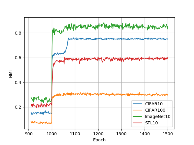
To illustrate the training phases of CoHiClust, we show the learning curves in Figure 5. Up to epoch 1000, we only trained the backbone model. Since in the pre-training phase, the clustering tree returns random decisions, we get a very low NMI value. After that, we start optimizing the CoHiLoss, and the NMI rapidly grows. In epoch 1050, we have a pruning phase, which results in further improvement of the NMI score. As can be seen, the model stabilizes its performance just after the pruning stage, which suggests that we can stop the training in epoch 1100. In conclusion, CoHiClust requires less than 100 epochs to obtain an optimal clustering score given a pre-trained model.

Figure 5: Learning curves on the validation set of CIFAR-10. Pre-training is performed until epoch 1000 and pruning is applied in epoch 1050. The model stabilizes its performance quickly after pruning.

Comparison with agglomerative clustering

We show that our top layer responsible for constructing a decision tree is an important component of CoHiClust and cannot be replaced by alternative hierarchical clustering methods. For this purpose, we first train a backbone network with a typical self-supervised SimCLR technique. Next, we apply agglomerative clustering to the resulting representation. As can be seen in Table 5, agglomerative clustering gets very low results, which means that joint optimization of the backbone network and clustering tree using the proposed $\mathrm{CoHiLoss}{}$ is a significantly better choice. In consequence, the representation taken from a typical self-supervised learning model does not provide a representation, which can be clustered accurately using simple methods.

Table 5: Comparison with agglomerative clustering trained on the representation generated by the self-supervised learning model.

	NMI	ACC	ARI
Agglomerative clustering	0.265	0.363	0.147
CoHiClust	0.767	0.84	0.72

4.3 Comparison with hierarchical clustering methods

To our knowledge, DeepECT [26] is the only hierarchical clustering method based on deep neural networks. Following their experimental setup, we report the results on two popular image datasets, MNIST and F-MNIST, and consider classical hierarchical algorithms evaluated on the latent representation created by the autoencoder and IDEC [14]. In addition to the previous clustering metrics, we also use dendrogram purity (DP) [21, 40], which directly compares the constructed hierarchy with the ground-truth partition. It attains its maximum value of 1 if and only if all data points from the same class are assigned to some pure sub-tree.

Table 6: Comparison with hierarchical models in terms of DP, NMI and ACC (higher is better).

Method	MNIST			F-MNIST
	DP	NMI	ACC	DP	NMI	ACC
DeepECT	0.82	0.83	0.85	0.47	0.60	0.52
DeepECT + Aug	0.94	0.93	0.95	0.44	0.59	0.50
IDEC (agglomerative complete*)	0.40	0.86	0.85	0.35	0.58	0.53
AE + k-means (bisecting*)	0.53	0.70	0.77	0.38	0.52	0.48
CoHiClust	0.97	0.97	0.99	0.52	0.62	0.65

* To report DP for flat clustering models, we use (optimally selected) typical hierarchical algorithms to build a hierarchy on the obtained data representation.

The results summarized in Table 6 demonstrate that CoHiClust outperforms all baselines on both MNIST and F-MNIST datasets in terms of all metrics. Interestingly, DeepECT benefits from data augmentation in the case of MNIST, while on F-MNIST it deteriorates its performance. All methods except CoHiClust and DeepECT failed completely to create a hierarchy recovering true classes (see the DP measure), which confirms that there is a lack of powerful hierarchical clustering methods based on neural networks. The disproportion between the results obtained on MNIST and F-MNIST demonstrates that recovering true classes of clothes is a significantly more challenging task than recognizing handwritten digits.

5 Conclusion

We proposed a contrastive hierarchical clustering model CoHiClust, which suits well to clustering of large-scale image databases. The hierarchical structure constructed by CoHiClust provides significantly more information about the data than typical flat clustering models. In particular, we can inspect the similarity between selected groups by measuring their distance in the hierarchy tree and, in consequence, find super-clusters. Experimental analysis performed on typical clustering benchmarks confirms that the produced partitions are highly similar to ground-truth classes. At the same time, CoHiClust allows us to discover important patterns that have not been encoded in the class labels.

5.0.1 Acknowledgements

The research of P. Rola was supported by the National Science Centre (Poland), grant no. 2021/41/B/ST6/01370. The research of J. Tabor was supported by the National Science Centre (Poland), grant no. 2022/45/B/ST6/01117. The research of M. Śmieja was supported by the Foundation for Polish Science co-financed by the European Union under the European Regional Development Fund in the POIR.04.04.00-00-14DE/18-00 project carried out within the Team-Net program. For the purpose of Open Access, the author has applied a CC-BY public copyright licence to any Author Accepted Manuscript (AAM) version arising from this submission.

Appendix 0.A Experimental setup

Gray-scale images: MNIST and F-MNIST

We instantiate the backbone network $g$ using ResNet18. Projection head $\pi$ used for parameterizing decisions made by internal tree nodes is a single-layer network. The projection head $\phi$ used for applying regularization $R_{2}$ is an identity function (NT-Xent loss is applied on the output of backbone network). We run CoHiClust with 16 leaves (4 tree levels). CoHiClust is trained for 200 epochs of pre-training and 100 epochs of tree construction (pruning is performed in epochs 10-15) using a minibatch size of $256$.

Color images

For CIFAR-10, CIFAR-100 and ImageNet-10, we use ResNet50 as a backbone network. The remaining datasets of color images employed ResNet-34 network. Projection heads $\pi$ and $\phi$ are separate two-layer networks. For CIFAR-10 and CIFAR-100, we run CoHiClust with 32 leaves, while for the remaining datasets we use 16 leaves. CoHiClust is trained for 1000 epochs of pre-training and 500 epochs of tree construction using a minibatch size of $512$ for CIFAR-10, CIFAR-100 and STL-10. In case of ImageNet-10 and ImageNet-Dogs we used minibatch with size of $128$. Pruning starts after 50 epochs of tree construction and we remove one leaf per epoch.

Summary of datasets

Table 7 summarizes datasets used for evaluation.

Table 7: A summary of datasets.

Dataset	Split	Samples	Classes	Resolution
CIFAR-10	Train+Test	60 000	10	$32\times 32$
CIFAR-100	Train+Test	60 000	20	$32\times 32$
STL-10	Train+Test	13 000	10	$96\times 96$
ImageNet-10	Train	13 000	10	$224\times 224$
ImageNet-Dogs	Train	19 500	15	$224\times 224$

Augmentations

For all datasets, we applied four types of augmentations: random cropping, horizontal flip, color jittering, and grayscaling.

Appendix 0.B Dendrogram purity for datasets of color images

In Table 8, we present dendrogram purity obtained by CoHiClust for datasets of color images. This benchmark can be used to compare other hierarchical clustering models.

Table 8: Dendrogram purity on color images.

	DP
CIFAR-10	0.715
CIFAR-100	0.231
STL-10	0.530
ImageNet-10	0.895
ImageNet-Dogs	0.190

Appendix 0.C Additional results

We present hierarchies and distance matrices constructed for the remaining datasets in the following figures.

Figure 6: Tree hierarchy constructed for MNIST. Observe that neighboring leaves contain images of visually similar classes, e.g. 8 and 0; 4 and 9; 1 and 7. Such a property holds also for nodes in the upper levels of the tree – the left sub-tree contain digits with circular shapes, while the digits located in the right sub-tree consist of lines.

Figure 7: Tree hierarchy generated by CoHiClust for F-MNIST (images in the nodes denote mean images in each sub-tree). The right sub-tree contains clothes while the other items (shoes and bags) are placed in the left branch. Looking at the lowest hierarchy level, we have clothes with long sleeves grouped in the neighboring leaves. The same holds for clothes with designs. Observe that CoHiClust assigned white-colored t-shirts and dresses to the same cluster, while trousers are in the separate one. Small shoes such as sneakers or sandals are considered similar (neighboring leaves) and distinct from ankle shoes. Concluding, CoHiClust is able to retrieve meaningful information about image semantics, which is complementary to the ground truth classification.

Figure 8: Tree hierarchy generated by CoHiClust for STL-10

(a) MNIST

(b) F-MNIST

(c) STL-10

(d) ImageNet-10

(e) ImageNet-Dogs

(f) CIFAR-100

Figure 9: Distance matrices retrieved from the constructed hierarchies for ground truth classes.

References

- [1] Alaniz, S., Marcos, D., Schiele, B., Akata, Z.: Learning decision trees recurrently through communication. In: Proceedings of the IEEE/CVF Conference on Computer Vision and Pattern Recognition. pp. 13518–13527 (2021)
- [2] Barai, A., Dey, L.: Outlier detection and removal algorithm in k-means and hierarchical clustering. World Journal of Computer Application and Technology 5(2), 24–29 (2017)
- [3] Bengio, Y., Lamblin, P., Popovici, D., Larochelle, H.: Greedy layer-wise training of deep networks. In: Schölkopf, B., Platt, J., Hoffman, T. (eds.) Advances in Neural Information Processing Systems. vol. 19. MIT Press (2006)
- [4] Bhattacharyya, A.: On a measure of divergence between two multinomial populations. Sankhyā: the indian journal of statistics pp. 401–406 (1946)
- [5] Cai, D., He, X., Wang, X., Bao, H., Han, J.: Locality preserving nonnegative matrix factorization 9, 1010––1015 (2009)
- [6] Chang, J., Wang, L., Meng, G., Xiang, S., Pan, C.: Deep adaptive image clustering. In: Proceedings of the IEEE International Conference on Computer Vision (ICCV) (Oct 2017)
- [7] Chen, T., Kornblith, S., Norouzi, M., Hinton, G.: A simple framework for contrastive learning of visual representations. In: III, H.D., Singh, A. (eds.) Proceedings of the 37th International Conference on Machine Learning. Proceedings of Machine Learning Research, vol. 119, pp. 1597–1607. PMLR (13–18 Jul 2020), https://proceedings.mlr.press/v119/chen20j.html
- [8] Chopra, S., Hadsell, R., LeCun, Y.: Learning a similarity metric discriminatively, with application to face verification. In: 2005 IEEE Computer Society Conference on Computer Vision and Pattern Recognition (CVPR’05). vol. 1, pp. 539–546. IEEE (2005)
- [9] Dang, Z., Deng, C., Yang, X., Wei, K., Huang, H.: Nearest neighbor matching for deep clustering. In: Proceedings of the IEEE/CVF Conference on Computer Vision and Pattern Recognition. pp. 13693–13702 (2021)
- [10] Frosst, N., Hinton, G.: Distilling a neural network into a soft decision tree. arXiv preprint arXiv:1711.09784 (2017)
- [11] Gowda, K.C., Krishna, G.: Agglomerative clustering using the concept of mutual nearest neighbourhood. Pattern Recognition 10, 105–112 (1978)
- [12] Grill, J.B., Strub, F., Altché, F., Tallec, C., Richemond, P., Buchatskaya, E., Doersch, C., Avila Pires, B., Guo, Z., Gheshlaghi Azar, M., et al.: Bootstrap your own latent-a new approach to self-supervised learning. Advances in neural information processing systems 33, 21271–21284 (2020)
- [13] Guérin, J., Gibaru, O., Thiery, S., Nyiri, E.: Cnn features are also great at unsupervised classification. arXiv preprint arXiv:1707.01700 (2017)
- [14] Guo, X., Gao, L., Liu, X., Yin, J.: Improved deep embedded clustering with local structure preservation. In: Ijcai. pp. 1753–1759 (2017)
- [15] Guo, X., Liu, X., Zhu, E., Yin, J.: Deep clustering with convolutional autoencoders. In: International conference on neural information processing. pp. 373–382. Springer (2017)
- [16] He, K., Fan, H., Wu, Y., Xie, S., Girshick, R.: Momentum contrast for unsupervised visual representation learning. In: 2020 IEEE/CVF Conference on Computer Vision and Pattern Recognition (CVPR). pp. 9726–9735 (2020). https://doi.org/10.1109/CVPR42600.2020.00975
- [17] Hu, W., Miyato, T., Tokui, S., Matsumoto, E., Sugiyama, M.: Learning discrete representations via information maximizing self-augmented training. In: International conference on machine learning. pp. 1558–1567. PMLR (2017)
- [18] Huang, J., Gong, S., Zhu, X.: Deep semantic clustering by partition confidence maximisation. In: Proceedings of the IEEE/CVF Conference on Computer Vision and Pattern Recognition. pp. 8849–8858 (2020)
- [19] Ji, X., Henriques, J.F., Vedaldi, A.: Invariant information clustering for unsupervised image classification and segmentation. In: Proceedings of the IEEE International Conference on Computer Vision. pp. 9865–9874 (2019)
- [20] Kingma, D.P., Welling, M.: Auto-encoding variational bayes. arXiv preprint arXiv:1312.6114 (2013)
- [21] Kobren, A., Monath, N., Krishnamurthy, A., McCallum, A.: A hierarchical algorithm for extreme clustering. In: Proceedings of the 23rd ACM SIGKDD international conference on knowledge discovery and data mining. pp. 255–264 (2017)
- [22] Lakhani, J., Chowdhary, A., Harwani, D.: Clustering techniques for biological sequence analysis: A review. Journal of Applied Information Scienc 3(1), 14–32 (2015)
- [23] Li, Y., Hu, P., Liu, Z., Peng, D., Zhou, J.T., Peng, X.: Contrastive clustering. In: Proceedings of the AAAI Conference on Artificial Intelligence. vol. 35, pp. 8547–8555 (2021)
- [24] Li, Y., Hu, P., Liu, Z., Peng, D., Zhou, J.T., Peng, X.: Contrastive clustering. Proceedings of the AAAI Conference on Artificial Intelligence 35(10), 8547–8555 (May 2021), https://ojs.aaai.org/index.php/AAAI/article/view/17037
- [25] MacQueen, J.: Some methods for classification and analysis of multivariate observations 1, 281––297 (1967)
- [26] Mautz, D., Plant, C., Böhm, C.: Deep embedded cluster tree. In: 2019 IEEE International Conference on Data Mining (ICDM). pp. 1258–1263. IEEE (2019)
- [27] Mautz, D., Plant, C., Böhm, C.: Deepect: The deep embedded cluster tree. Data Science and Engineering 5(4), 419–432 (2020)
- [28] Miyato, T., Maeda, S.i., Koyama, M., Ishii, S.: Virtual adversarial training: a regularization method for supervised and semi-supervised learning. IEEE transactions on pattern analysis and machine intelligence 41(8), 1979–1993 (2018)
- [29] Murtagh, F., Contreras, P.: Algorithms for hierarchical clustering: an overview. Wiley Interdiscip Rev Data Min Knowl Discov 2(1), 86–97 (2012)
- [30] Naumov, S., Yaroslavtsev, G., Avdiukhin, D.: Objective-based hierarchical clustering of deep embedding vectors. In: AAAI. pp. 9055–9063 (2021)
- [31] Radford, A., Metz, L., Chintala, S.: Unsupervised representation learning with deep convolutional generative adversarial networks. arXiv preprint arXiv:1511.06434 (11 2015)
- [32] Śmieja, M., Warszycki, D., Tabor, J., Bojarski, A.J.: Asymmetric clustering index in a case study of 5-ht1a receptor ligands. PloS one 9(7), e102069 (2014)
- [33] Tanno, R., Arulkumaran, K., Alexander, D., Criminisi, A., Nori, A.: Adaptive neural trees. In: International Conference on Machine Learning. pp. 6166–6175. PMLR (2019)
- [34] Vincent, P., Larochelle, H., Lajoie, I., Bengio, Y., Manzagol, P.A.: Stacked denoising autoencoders: Learning useful representations in a deep network with a local denoising criterion. Journal of Machine Learning Research 11(110), 3371–3408 (2010)
- [35] Wan, A., Dunlap, L., Ho, D., Yin, J., Lee, S., Jin, H., Petryk, S., Bargal, S.A., Gonzalez, J.E.: Nbdt: neural-backed decision trees. arXiv preprint arXiv:2004.00221 (2020)
- [36] Wu, J., Long, K., Wang, F., Qian, C., Li, C., Lin, Z., Zha, H.: Deep comprehensive correlation mining for image clustering. In: Proceedings of the IEEE/CVF International Conference on Computer Vision (ICCV) (October 2019)
- [37] Wu, Z., Xiong, Y., Yu, S.X., Lin, D.: Unsupervised feature learning via non-parametric instance discrimination. In: Proceedings of the IEEE conference on computer vision and pattern recognition. pp. 3733–3742 (2018)
- [38] Xie, J., Girshick, R., Farhadi, A.: Unsupervised deep embedding for clustering analysis. In: International conference on machine learning. pp. 478–487. PMLR (2016)
- [39] Yang, J., Parikh, D., Batra, D.: Joint unsupervised learning of deep representations and image clusters. In: Proceedings of the IEEE conference on computer vision and pattern recognition. pp. 5147–5156 (2016)
- [40] Yang, R., Qu, D., Qian, Y., Dai, Y., Zhu, S.: An online log template extraction method based on hierarchical clustering. EURASIP Journal on Wireless Communications and Networking 2019(1), 1–12 (2019)
- [41] Zbontar, J., Jing, L., Misra, I., LeCun, Y., Deny, S.: Barlow twins: Self-supervised learning via redundancy reduction. In: International Conference on Machine Learning. pp. 12310–12320. PMLR (2021)
- [42] Zeiler, M.D., Krishnan, D., Taylor, G.W., Fergus, R.: Deconvolutional networks. In: 2010 IEEE Computer Society Conference on Computer Vision and Pattern Recognition. pp. 2528–2535 (2010)
- [43] Zelnik-Manor, L., Perona, P.: Self-tuning spectral clustering. In: Advances in Neural Information Processing Systems. vol. 17. MIT Press (2004)
- [44] Zhang, F., Li, L., Hua, Q., Dong, C.R., Lim, B.H.: Improved deep clustering model based on semantic consistency for image clustering. Knowledge-Based Systems 253, 109507 (2022). https://doi.org/https://doi.org/10.1016/j.knosys.2022.109507, https://www.sciencedirect.com/science/article/pii/S0950705122007560
- [45] Zhang, Y., Ahmed, A., Josifovski, V., Smola, A.: Taxonomy discovery for personalized recommendation. In: Proceedings of the 7th ACM international conference on Web search and data mining. pp. 243–252 (2014)
- [46] Zou, Q., Lin, G., Jiang, X., Liu, X., Zeng, X.: Sequence clustering in bioinformatics: an empirical study. Briefings in bioinformatics 21(1), 1–10 (2020)