Self-supervised Sequential Information Bottleneck for Robust Exploration in Deep Reinforcement Learning
Abstract
Effective exploration is critical for reinforcement learning agents in environments with sparse rewards or high-dimensional state-action spaces. Recent works based on state-visitation counts, curiosity and entropy-maximization generate intrinsic reward signals to motivate the agent to visit novel states for exploration. However, the agent can get distracted by perturbations to sensor inputs that contain novel but task-irrelevant information, e.g. due to sensor noise or changing background. In this work, we introduce the sequential information bottleneck objective for learning compressed and temporally coherent representations by modelling and compressing sequential predictive information in time-series observations. For efficient exploration in noisy environments, we further construct intrinsic rewards that capture task-relevant state novelty based on the learned representations. We derive a variational upper bound of our sequential information bottleneck objective for practical optimization and provide an information-theoretic interpretation of the derived upper bound. Our experiments on a set of challenging image-based simulated control tasks show that our method achieves better sample efficiency, and robustness to both white noise and natural video backgrounds compared to state-of-art methods based on curiosity, entropy maximization and information-gain.
Index Terms:
Reinforcement learning, representation learning, exploration, intrinsic motivation, information bottleneck.1 Introduction
Deep reinforcement learning has achieved impressive success in complex environments, including navigation [1, 2], manufacturing [3, 4, 5] and healthcare [6]. Reinforcement learning agents learn an optimal policy by maximizing the external reward while interacting with the environment. A fundamental challenge in reinforcement learning, commonly referred to as the exploration-exploitation dilemma [7, 8], is to trade off between exploring different solutions to maximize reward, and improving the current best solution. Auxiliary rewards for intrinsic motivation are often used to guide exploration, which is in particular important for environments with sparse rewards or high-dimensional state-action spaces [9, 10].
Constructing auxiliary reward signals based on the novelty of the states has been shown to be effective [11, 12, 13]. State novelty can be quantified based on state-visitation counts [14, 15, 16], prediction errors of dynamic models [17, 18, 19], or based on the entropy of the state distribution induced by the agent’s policy [20, 21]. While these approaches utilize the generated intrinsic reward to encourage the agent to explore novel states, they often fail to capture task-specific state novelty in the presence of perturbations, since they have no incentive to filter out novel but distractive information (e.g., due to noise or changes in the background). For example, using the predictive error of a dynamic model as an intrinsic reward motivates the agent to choose actions that cause surprising transitions even if they are only surprising with respect to task-irrelevant information.
The information bottleneck principle [22] provides a useful insight in extracting task-relevant information from raw states. Specifically, the information bottleneck aims to obtain a sufficient and maximally compressed representation from the raw input given the target variable by maximizing the predictive information and meanwhile minimizing the mutual information between the input and the compressed representation, that is,
| (1) |
where is a positive coefficient for trading off both objectives. Some recent approaches directly apply the information bottleneck to learn compressed representations from raw states for measuring the task-specific state novelty for guiding exploration [23, 24, 25].
However, the original information bottleneck principle is only suitable for compressing individual observations and fails to model the temporal information gain within the sequential observations of a reinforcement learning agent. Instead, modelling and compressing temporal information gain in time-series observations may enable the agent to learn compressed representations that capture the temporal correlations and long-term dependencies between observations at multiple time steps, which may help the agent to better understand the consequences of its actions. Moreover, measuring the state novelty on the obtained compressed representation could be used to filter out task-irrelevant information for efficient exploration in noisy environments.
Hence, in this paper we propose a sequential information bottleneck method to quantify task-relevant state novelty for exploration, SIBE, which learns compressed and temporal-coherent representations by modelling and compressing information gain in a sequence of state representations. Specifically, our method maximizes the predictive information between sequential latent bottleneck variables while minimizing the mutual information between a sequence of compact state representations and bottleneck variables for compression. We derive an upper bound of our sequential information bottleneck objective using variational inference for computationally feasible optimization, and provide an information-theoretic interpretation of the derived upper bound. Furthermore, we construct an auxiliary reward function in the learned latent space of bottleneck variables for guiding exploration. Our reward function measures the state novelty by the InfoNCE bound [26] on the temporal predictive information between the current bottleneck variable and action and the next bottleneck variable. The agent receives the intrinsic reward when it encounters latent states with high InfoNCE loss, which indicates that the task-relevant aspects of the states—encoded by the learned bottleneck variables—are hard to predict by our model. To the best of our knowledge, our method is the first that models and compresses the overall predictive information in sequential observations for exploration in reinforcement learning problems.
We train our sequential information bottleneck model along with a standard soft actor-critic [27] reinforcement learning agent for learning a policy from high-dimensional states. We conduct extensive experiments on a set of challenging image-based continuous control tasks, including standard Mujoco tasks, and Mujoco tasks with distractive backgrounds, where we use both, white noise and natural videos. We summarize our contributions as follows:
-
•
We introduce the sequential information bottleneck objective and use it for compressing the overall predictive information in a sequence of observations, which enables us to learn compressed and temporal-coherent bottleneck representations from time-series observations.
-
•
We derive a variational upper bound of our sequential information bottleneck objective for practical optimization, and provide an interpretation of our derived upper bound from the perspective of information theory.
-
•
We propose an intrinsic reward function based on the InfoNCE bound on the temporal predictive information of the bottleneck variables, which quantifies the task-relevant state novelty for guiding exploration.
-
•
Empirical evaluations show that our method achieves better sample efficiency on standard Mujoco tasks, while also being more robust to both noisy and natural video backgrounds compared to state-of-the-art baselines based on prediction-error, entropy-maximization or information-gain.
The remainder of the paper is organized as follows. In Section 2, we discuss previous exploration methods based on intrinsic reward. In Section 3, we present the proposed sequential information bottleneck objective and the intrinsic reward function for exploration. We show the implementation of our method and the experimental results on the benchmark tasks in Section 4. In Section 5, we draw a conclusion and discuss limitations and future work.
2 Related Work
Several prior works on exploration use an intrinsic motivation mechanism that quantifies the novelty of states for guiding exploration [17, 12, 28, 23]. An intuitive approach for providing a measure of novelty is to compute the pseudo-counts of state visitations. For example, Bellemare et al. [14] and Ostrovski et al. [15] estimate pseudo-counts based on density models over the state space and subsequently use a function of state visitation count as intrinsic reward. Tang et al. [29] use a hash table to transform visited states into hash codes and then compute the state visitation counts based on the hash table. An alternative approach for estimating state novelty is curiosity-driven exploration [30], which uses the prediction error of a dynamics model as novelty measurement and encourages the agent to explore the unpredictable parts of the environment. For instance, ICM [17] builds forward and inverse dynamic models in the latent space and uses the prediction error of the forward model as intrinsic motivation. The generated intrinsic rewards encourage the agent to visit states with large prediction errors. Plan2Explore [18] uses an ensemble of environment models to compute the disagreement in the next predicted state embedding and then use this disagreement as intrinsic reward. EMI [13] learns a latent state space via maximizing the mutual information between state and action embeddings, and subsequently imposes linear dynamics on the learned latent space. The prediction error of the linear dynamic model serves as intrinsic reward for exploration. However, these aforementioned count-based and curiosity-driven exploration methods have no incentive to remove novel but task-irrelevant information from observations, such as white-noise. Hence, they can capture task-irrelevant state novelty and therefore mislead exploration.
Entropy-based exploration methods maximize the entropy of the state distribution to encourage the agent to visit novel states. For example, Hazan et al. [12] employ a concave function of the policy-induced state distribution as intrinsic reward function. APT [31] uses a particle-based estimate of the state entropy and maximizes this estimate to guide exploration. The particle-based entropy estimator is based on the averaged distance between each state representation and its k-nearest neighbor. Similar to APT, Proto-RL [20] learns an encoder to transform image observations into a low-dimensional latent space along with a set of prototypical embeddings. A k-nearest-neighbor entropy estimator computed over latent state embeddings and prototypical embeddings approximates the state entropy for exploration. However, these methods based on entropy maximization are sensitive to state noise and can, thus, fail for noisy environments, since the state entropy is easily affected by random noises in the state space.
Some pioneering methods apply the information bottleneck principle to distill task-relevant information from observations and then capture task-relevant state novelty for boosting exploration. For instance, Tao et al. [25] use many auxiliary tasks to shape the representation space and then learn a latent dynamic model based on the information bottleneck principle. They define an intrinsic reward function by measuring the average distance between the state embedding and its k-nearest-neighbors. Kim et al. [24] maximize the mutual information between the current state representation and its target value while minimizing the mutual information between the current state and its representation for compression. They subsequently use the information gain between the current state and its representation as an intrinsic reward for guiding exploration. More recently, DB [23] learns compressed dynamic-relevant representations via the information bottleneck principle and encourage the agent to explore novel state-action pairs with high information gain. In contrast, our method aims to compress a sequence of state representations, which generates a sequence of bottleneck variables for capturing compressed prediction information over multiple time steps. Our sequential information bottleneck is significantly different from existing (non-sequential) information bottleneck methods [25, 23, 24], which only compress individual states or state representations.
Sequential mutual information was already used for robust predictable control (RPC [32]). Eysenbach et al. [32] maximize external rewards while minimizing the sequential mutual information between the states and the latent representations used by the policy, for limiting the amount of observed information that affects the agent’s behavior. However, our self-supervised sequential information bottleneck objective not only learns a compressed representation, but also retains predictive information within the sequence of latent representations, which enables us to capture temporal correlations in latent sequential representations.
Our work is also related to unsupervised representation learning methods based on mutual information estimation [33, 34]. Laskin et al. [35] apply two independent data augmentations on the same state and maximize the mutual information between the corresponding representations for learning compact state representations, while Oord et al. [26] learn state representations by maximizing the mutual information between consecutive states. Moreover, Lee et al. [36] use the conditional entropy bottleneck to maximize the mutual information between the current embedding and the future state and reward, while minimizing the mutual information between the current state and the state embedding. In contrast to these methods, our method captures the compressed predictive information within multiple time steps for shaping the latent state space, and moreover, provides a useful reward signal for exploration. To the best of our knowledge, our approach is the first to compress and preserve the predictive information over a sequence of states for guiding exploration in reinforcement learning.
3 Sequential Information Bottleneck
In this section, we formulate our objective of compressing sequential state representations and derive a practical optimization objective based on variational inference. We also describe how to generate intrinsic rewards based on the InfoNCE bound [26], and how our method can be integrated with soft actor-critic [27].
3.1 Preliminaries and Notation
We consider a Markov decision process (MDP) formulated by the tuple , where is the state space, is the action space, is the stochastic dynamic model, is the reward function and is the discount factor. At each time step, the agent observes the current state and selects its actions based on its stochastic policy , and then receives the reward . The reinforcement learning objective is to maximize the expected cumulative rewards where denotes the agent’s trajectory. We focus on image-based reinforcement learning, where the state space is in the form of images. We do not explicitly consider partial observability of single image observations, but assume that stacking the most recent images yields a high-dimensional but Markovian state where is the observed image at time step .
3.2 The Sequential Information Bottleneck Objective
We propose the sequential information bottleneck model, SIBE, for compressing predictive information over a sequence of state representations. We first map a sequence of high-dimensional states into compact state representations using a deterministic convolutional network. We further use a parameterized stochastic neural network that takes state representations as input and randomly outputs latent samples . The goal of SIBE is to find maximally compressed and temporal coherent representations given a sequence of state representations .
Following the original information bottleneck principle [22], the proposed objective of SIBE aims to compress the mutual information between and while preserving sufficient predictive information between latent variables , by solving the optimization problem,
| (2) |
where is a positive coefficient for controlling the compression-relevance trade-off. Intuitively, minimizing the sequential mutual information allows us to filter out overall task-irrelevant information from a sequence of state representations , e.g. white noise or irrelevant backgrounds. Meanwhile, the sequential predictive information measures the overall interdependency between latent bottleneck variables . Maximizing the predictive information forces the latent bottleneck variable to capture the overall dependency for joint compression of . This is the key difference to previous information-bottleneck based methods [23, 24, 25] that only perform individual compression on single observations. Moreover, unlike the original information bottleneck principle, our sequential information bottleneck objective is a self-supervised objective by encouraging the latent bottleneck variables to predict themselves, which eliminates the need to give an explicit target .
3.3 Algorithm Overview

Unfortunately, optimizing the sequential information bottleneck directly is computationally intractable. Hence, we derive an upper bound of Eq. 2 by upper-bounding the sequential mutual information and lower-bounding the sequential predictive information . We use our upper bound as an auxiliary loss during reinforcement learning for learning compressed representations for policy and Q-function. Furthermore, we build an intrinsic reward for guiding exploration.
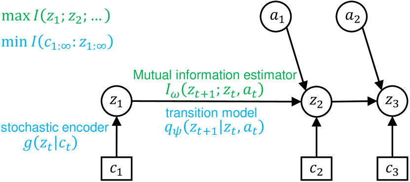
Before showing the concrete loss functions, the reward function and their derivations, we provide an overview of the proposed network architecture in Fig. 1. We use an online deterministic encoder with parameters to extract the compact state representation from the state at the current time step. An online stochastic encoder with parameters is used to map the state representation into mean and standard deviation of a diagonal Gaussian distribution , which is used for sampling the bottleneck variable. The sampled bottleneck variable and action are fed into a transition model with parameters , which outputs the mean and standard deviation of a variational Gaussian distribution which is trained to predict the embedding at the next time step. A projection head with parameters and an online prediction head with parameters are used to introduce a nonlinear transformation to the bottleneck variable and action for computing the InfoNCE loss, which will be introduced during the derivation of the lower bound of the sequential predictive information .
However, when determining the next state representation and latent bottleneck representation , we use target networks for preventing gradients to flow through the deterministic and stochastic encoders. We also use a target prediction head without gradient flow when introducing a nonlinear transformation of the next representation for the InfoNCE loss. In contrast to the online deterministic encoder with parameters , the online stochastic encoder with parameters and the online prediction head with parameters , the respective parameters of the target networks (, and ) are not optimized with respect to our objective functions, but follow their online counterparts using an exponential moving average [37],
| (3) | ||||
where is the coefficient of the exponential moving average. Target networks can efficiently avoid mode collapse, as shown in prior studies [37, 35]. The state representations and their corresponding latent bottleneck representations are, hence, created using the models,
| (4) | ||||||
3.4 Maximizing a Lower Bound of
We will now construct a lower bound on the mutual information suitable for optimization. We first introduce the conditional distribution to the definition of multivariate mutual information ,
| (5) | ||||
where is the joint distribution of and . The inequality directly follows from the non-negativity of the KL divergence.
Without loss of generality, we can write the conditional distribution in its autoregressive form,
| (6) |
We plug Eq. 6 into Eq. 5 to obtain
| (7) | ||||
where the expectation is computed over the distribution . For tractability, we further use the conditional distribution instead of , which is an approximation due to the non-Markovianity of the learned embeddings. Our objective, however, remains a lower bound of the true mutual information ,
| (8) | ||||
This derivation shows that the multivariate mutual information can be lower-bounded by the sum of the mutual information between the current bottleneck variable and action , and the next bottleneck variable . The term measures overall predictive information that all latent representations share over time, which can be interpreted as the \sayglobal information gain associated with the sequence of bottleneck variables . The term quantifies the predictive information between individual transition of bottleneck variables , which can be interpreted as the \saylocal information gain related to the environment dynamics. Maximizing the \sayglobal predictive information is equivalent to maximizing a sum of the \saylocal mutual information, which encourages latent bottleneck variables to preserve sufficient relevant information for future prediction. Eq. 8 simplifies the complex multivariate mutual information objective into a sum of computationally simpler mutual information objective .
For maximizing the lower bound of (Eq. 8), we employ the InfoNCE lower bound [26] on the local mutual information terms . Specifically, let denote samples randomly sampled from the joint distribution which we refer to positive sample pairs, and let denote a set of negative samples drawn from the marginal distribution . Then, the InfoNCE loss for maximizing the lower bound of is given as
| (9) |
where is the score function and the expectation is computed with respect to the joint distribution of , and , and the negative sample sets. Minimizing the InfoNCE loss is equivalent to maximizing the lower bound on the mutual information . The score function transforming feature variables into scalar-valued scores is given by
| (10) |
Here the function concatenates and and is a learnable weight transformation matrix. The projection head and the online prediction head are utilized to nonlinearly transform , while using the target prediction head to introduce a nonlinear transformation to . By maximizing the inner product between the nonlinear transformations of and , the InfoNCE loss with the score function forces our model to learn temporally predictive bottleneck variables.
To compute the lower bound of the sequential mutual information (Eq. 8), we need to maximize the sum of over multiple time steps. In practice, we randomly draw a minibatch of sequence chunks with chunk length from the replay buffer. As our lower bound (Eq. 8) decomposes into additive loss terms for different time steps, the only effect of sampling trajectory chunks, is to ensure that the minibatch contains subsequent time steps. We will show in Section 4.5, that ensuring at least two sequential transitions in the minibatch significantly improves the performance. We acquire a minibatch of sequence chunks of positive sample pairs by feeding into our network architecture. For time step to , we construct a negative sample set for a given positive sample pair by replacing with all from other sample pairs in the same minibatch.
3.5 Minimizing an Upper Bound of
For obtaining an upper bound on the sequential mutual information , we introduce a parametric variational distribution to approximate the marginal distribution ,
| (11) | ||||
where the expectation is computed over the distribution , and denotes the Gaussian distribution of the bottleneck variable given state representation at the initial step. The inequality in Eq. 11 follows from the non-negativity of the KL divergence. Following [32], we parameterize our variational distribution as
| (12) |
with Gaussian distributions and .
We then plug Eq. 12 to Eq. 11 to obtain our upper bound on the sequential mutual information,
| (13) | ||||
which is given in terms of KL divergences between our stochastic encoder and the transition model, encouraging the variational distribution to approximate the dynamics of the bottleneck variable . The term measures the uncertainty of given , which can be interpreted as the unavoidable information cost for encoding into . The term measures the uncertainty of given and , which can be regarded as the information gain, encouraging the bottleneck variable to predict the future well. Hence, the first term in Eq. 13 can be interpreted as the sum of information gain and cost over time steps. The last term in Eq. 13 measures the sum of information gain and cost at the first step. Although we could store the time steps in the replay buffer and treat the first time step separately by using an unconditional variational distribution , we omit this term for simplifying the implementation. For each sample in our minibatch, we compute the KL divergence analytically based on the means and standard deviations of two diagonal Gaussian distribution and , that is
| (14) | ||||
To minimize the KL divergence over multiple consecutive time steps, we use the same minibatch of sequence chunks that we use for optimizing Eq. 8.
3.6 The Loss Function and Optimization
Based on our bounds on the sequential mutual information and the sequential predictive information , we minimize the sequential information bottleneck (Eq. 2) by minimizing the upper bound
| (15) | ||||
The derived upper bound contains a summation over time steps and enables us to preserve and compress predictive information in time-series observations. We optimize the upper bound via sampling during training. The parameters of the online deterministic encoder , the online stochastic encoder , the latent transition model , the projection head , the online prediction head and the weight transformation matrix are simultaneously optimized by minimizing this loss function. We show the generative process of learned sequential bottleneck variables in Fig.2.
3.7 Intrinsic Reward for Exploration
By minimizing the upper bound (Eq. 15), we can induce a compact latent space of bottleneck variables which filters out distractive information. In this section, we discuss how we can use the task-specific novelty in the learned latent space for guiding exploration. Our intrinsic reward function is based on curiosity-driven exploration [17] where the agent is driven to visit novel states with high prediction errors. The agent is only rewarded when it encounters states that are hard to predict. The InfoNCE loss measures how difficult the next bottleneck variable is for the agent to predict given the current bottleneck variable and the action . The agent cannot accurately predict the future bottleneck variables with large InfoNCE loss. Therefore, we propose to use the InfoNCE loss on bottleneck variables as an intrinsic reward to encourage the agent to explore novel states. The intrinsic reward at the current time step is given by
| (16) |
where the expectation is computed with respect to the distribution and is a scaling factor. Intuitively, the intrinsic rewards encourage the agent to choose the actions that result in transitions that our model is not able to predict well. Combing the environment reward with the intrinsic reward , we obtain the augmented reward
| (17) |
3.8 Plugging into a Reinforcement Learning algorithm
We train our representation jointly with a soft actor-critic agent [27]. The training procedure is presented in Algorithm 1. The algorithm alternates between collecting new experience from the environment, and updating the parameters of the SIBE model, the actor and critic networks of SAC. The actor takes the deterministic state representations computed with the online deterministic encoder as input and select actions. We let the gradients of the critic backpropagate through the online deterministic encoder, since the environment reward can provide useful task-relevant information. We stop the gradient of the actor through the embedding, since this can degrade performance by implicitly modifying the Q-function during the actor update [38].
4 Experimental Evaluation
4.1 Experimental Setup
We evaluate the proposed algorithm SIBE on a set of challenging standard Mujoco tasks from the Deepmind control suite [39] (Fig. 3 top row). Specifically, we evaluate our method in six continuous control Mujoco tasks with high-dimensional observations: 1) in the Ball-in-cup Catch task, the agent is only provided with a sparse reward when the ball is caught, 2) in the Cartpole Swingup-sparse task, the agent obtains a sparse reward for bringing the unactuated pole close to the upright position, 3) in the Reacher Easy task, the agent obtains sparse reward for reaching the target location, 4) in the Cartpole Swingup task the agent obtains images from a fixed camera and may move out of sight, 5) in the Walker Walk and 6) Cheetah Run tasks the agent needs to control a robot with large action dimensions and complex dynamics due to ground control. Every task poses a set of challenges for learning an optimal policy, including sparse rewards, high-dimensional states, contacts and complex dynamics.
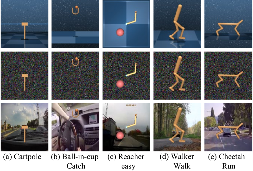
We further carry out our evaluation in two more settings for testing the robustness of our algorithm: the noisy setting and the natural video setting. We refer to Mujoco tasks in the noisy setting and the natural video setting as noisy Mujoco tasks and natural Mujoco tasks, respectively. The image observations of standard Mujoco tasks (Fig. 3 top row) from the Deepmind control suite only have simple backgrounds (see Fig. 3 top row). In the noisy setting, each background image (see Fig. 3 middle row) is filled with pixel-wise Gaussian white noise that is regarded as a strong state distractor for reinforcement learning tasks [40, 23]. Furthermore, in order to simulate robots in natural environments with complex observations, in the natural video setting (see Fig. 3 bottom row) the background of the Mujoco tasks is replaced by natural videos [41, 42] sampled from the Kinetics dataset [43]. The backgrounds of natural Mujoco tasks are continuously changing during training and evaluation, which introduces realistic and strong perturbations to observation images.
We compare SIBE with the following leading baselines for exploration in our experiments: 1) Proto-RL [20], an entropy maximization exploration method which measures the state entropy using prototypical representations and builds an entropy-based intrinsic reward for exploration, 2) DB [23], which learns dynamic-relevant compressed representations by using an information bottleneck objective and constructs an intrinsic reward signal to encourage the agent to explore novel states with high information gain, 3) Plan2Explore [18], a curiosity-driven exploration method which utilizes the disagreement in the predicted next state representations as intrinsic rewards, 4) RPC [32], which constructs an information-theoretic intrinsic reward function for encouraging the agent to learn a simple policy that uses few bits of information. We use the same codebase of the SAC algorithm for DB, Proto-RL and RPC to ensure a fair comparison to other model-free methods, while following the original implementation of the model-based method Plan2explore. The implementation details of our method are available in Appendix A.
The performance of each algorithm is evaluated by computing an average return over 10 episodes every 10K environment steps. For each method, the agent performs one gradient update per environment step for all tasks to ensure a fair comparison. For a more reliable comparison, we run each algorithm with five different random seeds for each task. All figures plot the average reward over these seeds, together with 95% confidence shading.
4.2 Sample Efficiency
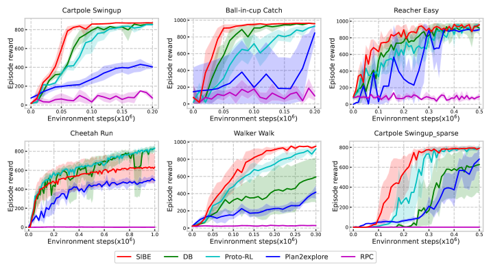
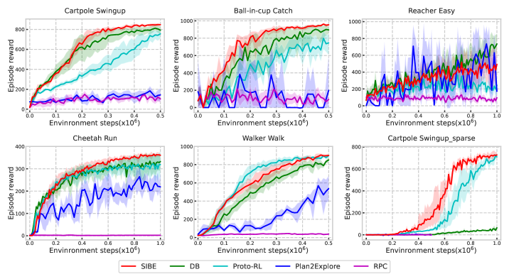
In this section, we investigate whether SIBE can succeed in challenging benchmark tasks. Fig. 4 compares our algorithm with DB, Proto-RL, Plan2explore and RPC on six standard Mujoco tasks from the Deepmind control suite. SIBE achieves better sample efficiency compared to all baselines on five out of six tasks. The results indicate that the compressed representations and the intrinsic reward learned by SIBE significantly help to learn good policies on challenging image-based tasks.
| 500K step scores | SIBE(Ours) | DB | Proto-RL | Plan2Explore | RPC | ||||
| Noisy Mujoco tasks | Cartpole Swingup | 867 8∗ | 858 5 | 845 5 | 79723 | 10213 | |||
| Ball-in-cup Catch | 966 2∗ | 602 187 | 926 8 | 95110 | 4121 | ||||
| Reacher Easy | 959 17∗ | 945 18 | 954 18 | 951 7 | 9113 | ||||
| Cheetah Run | 330 10∗ | 273 26 | 267 4 | 253 14 | 21 | ||||
| Walker Walk | 943 7 ∗ | 869 38 | 904 19 | 74232 | 251 | ||||
| Cartpole Swingup-sparse | 750 13∗ | 503 119 | 595 73 | 625 41 | 0 0 | ||||
| Natural Mujoco tasks | Cartpole Swingup | 848 5∗ | 793 18 | 756 21 | 14334 | 10319 | |||
| Ball-in-cup Catch | 954 6∗ | 896 20 | 746 63 | 198177 | 5524 | ||||
| Reacher Easy | 387 48 | 396 70 | 283 45 | 529 196∗ | 98 12 | ||||
| Cheetah Run | 314 15∗ | 293 17 | 29210 | 232 27 | 2 1 | ||||
| Walker Walk | 901 12∗ | 852 17 | 899 10 | 53673 | 383 | ||||
| Cartpole Swingup-sparse | 169 54∗ | 1 1 | 46 7 | 0 0 | 0 0 | ||||
4.3 Robustness to Noisy Observations
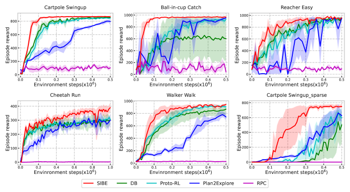
To study whether our method is robust in the presence of white noise, we corrupt the image observations in the Mujoco tasks (Fig. 3 middle row) with random Gaussian white noise, which introduces random task-irrelevant patterns to the raw observations. Fig. 5 compares the robustness of SIBE against DB, Proto-RL, Plan2explore and RPC on six noisy Mujoco tasks. SIBE outperforms all baselines on all six tasks in terms of robustness to noisy observations. Moreover, we observed that the performance of our method remains consistent when handling noisy Mujoco tasks, whereas the baselines show a clear decline in performance. For example, SIBE achieves similar performance in standard and noisy Ball-in-cup Catch and Cartpole Swingup-sparse tasks, while the performance of strong baselines DB and Proto-RL clearly decrease in presence of Gaussian white noise.
Following previous work [35], in the top half of Table I, we also compare performance (mean and standard error) at a fixed number of environment interactions (e.g. 500K) on the noisy Mujoco tasks. SIBE achieves better asymptotic performance at 500K environment steps compared to the baselines across all tasks. The results in the noisy setting demonstrate that SIBE is robust to noisy observations.
4.4 Robustness to Natural Background
We further investigate the robustness of our method on the natural Mujoco tasks (Fig. 3 bottom row), where the natural backgrounds of the observations are constantly changing. As shown in Fig. 6, except for Reacher Easy, SIBE achieves better performance than the baselines.
The performance at 500K environment interactions is shown in the bottom half of Table I. Our method achieves better or at least comparable performance across all tasks compared to the baselines. Moreover, our algorithm maintains consistent performance on the majority of natural Mujoco tasks, while the performance of baselines (e.g. Proto-RL and Plan2Explore) drop dramatically. The experimental results in the natural video setting show that SIBE is robust to task-irrelevant changes in the background.

4.5 Ablation
We conduct ablation studies to analyze the individual contributions of each component in our model. In our ablation studies, we focus on three sparse-reward tasks, namely Ball-in-cup Catch, Reacher Easy and Cartpole Swingup-Sparse. We first investigate two ablations of our SIBE model: non-reward SIBE, which removes the intrinsic reward signal during policy learning and non-compression SIBE, which removes the first terms in Eq. 15 derived from the compression objective . Fig. 7 presents the performance of SIBE and its two ablations on the standard Cartpole Swingup-sparse task with raw images (left), white noise (middle) and natural video background (right). The results on all three sparse-reward tasks in each setting are provided in Appendix B. SIBE outperforms all ablations on all standard Mujoco tasks, the noisy Mujoco tasks, as well as the natural Mujoco tasks. More specifically, by comparing the performance of SIBE and non-reward SIBE, we observed using InfoNCE loss as intrinsic reward to encourage the agent to visit novel states helps to achieve better performance for all settings. Moreover, the performance gain achieved by SIBE compared to non-compression SIBE indicates that compressing sequential observations improves the performance, especially in Mujoco tasks with distractive information (both white noise and natural video backgrounds).
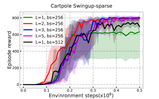
We also tested whether preserving and compressing predictive information in a sequence of observations improves the performance compared to using individual transitions, which only involves two time steps. Whereas, in all previous experiments we used the fixed chunk length , in the following experiments we evaluate the performance of SIBE when using different chunk lengths for sampling from the replay buffer. When the chunk length is set to 1, SIBE only uses individual transitions. We show the performance of SIBE for 4 different chunk lengths on the standard Cartpole Swingup-sparse task in Fig. 8 and additional results on three reward-sparse tasks in Appendix B. Using at least two sequential transitions outperforms SIBE with chunk length on all three tasks. As the number of data samples increases when increasing the chunk length , we also ran an experiment with and doubled batch size for the SIBE loss. The only difference to our experiment with is that the latter guarantees that the minibatch contains consecutive time steps. We conclude that capturing compressed predictive information in sequential observations helps to improve the performance compared to only compressing individual transitions.
4.6 Visualization
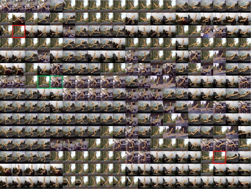
We visualize the learned representations by our method on natural Mujoco tasks using t-SNE [44] to gain more insights into the learned compressed embeddings. While t-SNE projects multidimensional representations into 2D plots, there tend to be many overlapping points in the 2D map. In order to avoid overlapping, we quantize t-SNE points into a 2D grid of size using RasterFairy [45]. In Fig. 9 we show the visualization of the representations learned by SIBE on the Walker Walk task with natural background. The latent space of the learned compressed representation organizes the variation in robot configurations even in presence of natural backgrounds. Specifically, images with similar robot configurations and clearly different backgrounds appear close to each other (e.g. the image pair marked by green square), while observations with different robot configurations but similar natural backgrounds are far away to each other (e.g. the two images marked by red square), indicating that the learned compressed representations Z meaningfully capture task-relevant information related to robot configurations, while filtering out task-irrelevant perturbations (e.g. changing natural background).
5 Conclusion and Discussion
We presented the sequential information bottleneck model, SIBE, for learning compressed and temporal-coherent bottleneck variables by preserving and compressing the overall predictive information over a sequence of observations. We further build intrinsic reward signals by measuring task-specific state novelty in the learned latent space of bottleneck variables for effective exploration in noisy environments. We optimize our model by deriving an upper bound on the sequential information bottleneck objective using variational inference. Empirical evaluations on a set of challenging image-based standard Mujoco tasks show that SIBE achieves better sample efficiency than the baselines on the majority of tasks, outperforming curiosity based, entropy-maximization based and information-gain based methods. Furthermore, we evaluate the performance of our method on complex Mujoco tasks with noisy and natural video backgrounds. The results demonstrate that our method is more robust to observations with both white noise and natural video backgrounds compared to the baselines.
Although SIBE outperforms the baseline in a set of challenging images-based benchmark tasks, our method slightly increases the computation time during policy learning, since we require to sample a minibatch of sequence chunks from the replay buffer. In addition, our method only focuses on extracting task-relevant information from pure visual data and lacks a mechanism to compress predictive information in multimodal sensory data. Utilizing and compressing the redundant information in multiple sensory modalities to further improve the robustness is a natural extension of our work. Our future work also considers extending the sequential information bottleneck objective into other types of time-series data, such as video or natural language.
Acknowledgments
Bang You gratefully acknowledges the financial support from China Scholarship Council Scholarship program (No.202006160111).
References
- [1] X. Wang et al., “Vision-language navigation policy learning and adaptation,” IEEE Trans. Pattern Anal. Mach. Intell., vol. 43, no. 12, pp. 4205–4216, 2020.
- [2] Y. Zhu et al., “Target-driven visual navigation in indoor scenes using deep reinforcement learning,” in Proc. IEEE Int. Conf. Robot. Autom., 2017, pp. 3357–3364.
- [3] N. Funk, G. Chalvatzaki, B. Belousov, and J. Peters, “Learn2assemble with structured representations and search for robotic architectural construction,” in Proc. Annu. Conf. Robot Learn. PMLR, 2022, pp. 1401–1411.
- [4] M. A. Lee et al., “Making sense of vision and touch: Learning multimodal representations for contact-rich tasks,” IEEE Trans. Robot., vol. 36, no. 3, pp. 582–596, 2020.
- [5] Z. Hou, J. Fei, Y. Deng, and J. Xu, “Data-efficient hierarchical reinforcement learning for robotic assembly control applications,” IEEE Trans. Ind. Electron., vol. 68, no. 11, pp. 11 565–11 575, 2020.
- [6] A. Guez, R. D. Vincent, M. Avoli, and J. Pineau, “Adaptive treatment of epilepsy via batch-mode reinforcement learning.” in Proc. AAAI Conf. Artif. Intell., 2008, pp. 1671–1678.
- [7] R. S. Sutton and A. G. Barto, Reinforcement learning: An introduction. Cambridge, MA, USA: MIT press, 2018.
- [8] R. Kumaraswamy, M. Schlegel, A. White, and M. White, “Context-dependent upper-confidence bounds for directed exploration,” Proc. Int. Conf. Neural Inf. Process. Syst., vol. 31, 2018.
- [9] R. Houthooft, X. Chen, Y. Duan, J. Schulman, F. De Turck, and P. Abbeel, “Vime: Variational information maximizing exploration,” Proc. Int. Conf. Neural Inf. Process. Syst., vol. 29, 2016.
- [10] N. Ratzlaff, Q. Bai, L. Fuxin, and W. Xu, “Implicit generative modeling for efficient exploration,” in Proc. Int. Conf. Mach. Learn. PMLR, 2020, pp. 7985–7995.
- [11] E. Conti, V. Madhavan, F. Petroski Such, J. Lehman, K. Stanley, and J. Clune, “Improving exploration in evolution strategies for deep reinforcement learning via a population of novelty-seeking agents,” Proc. Int. Conf. Neural Inf. Process. Syst., vol. 31, 2018.
- [12] E. Hazan, S. Kakade, K. Singh, and A. Van Soest, “Provably efficient maximum entropy exploration,” in Proc. Int. Conf. Mach. Learn. PMLR, 2019, pp. 2681–2691.
- [13] H. Kim, J. Kim, Y. Jeong, S. Levine, and H. O. Song, “Emi: Exploration with mutual information,” in Proc. Int. Conf. Mach. Learn. PMLR, 2019, pp. 3360–3369.
- [14] M. Bellemare, S. Srinivasan, G. Ostrovski, T. Schaul, D. Saxton, and R. Munos, “Unifying count-based exploration and intrinsic motivation,” Proc. Int. Conf. Neural Inf. Process. Syst., vol. 29, 2016.
- [15] G. Ostrovski, M. G. Bellemare, A. Oord, and R. Munos, “Count-based exploration with neural density models,” in Proc. Int. Conf. Mach. Learn. PMLR, 2017, pp. 2721–2730.
- [16] J. Martin, S. S. Narayanan, T. Everitt, and M. Hutter, “Count-based exploration in feature space for reinforcement learning,” in Proc. 26th Int. Joint Conf. Artif. Intell., 2017, pp. 2471–2478.
- [17] D. Pathak, P. Agrawal, A. A. Efros, and T. Darrell, “Curiosity-driven exploration by self-supervised prediction,” in Proc. Int. Conf. Mach. Learn. PMLR, 2017, pp. 2778–2787.
- [18] R. Sekar, O. Rybkin, K. Daniilidis, P. Abbeel, D. Hafner, and D. Pathak, “Planning to explore via self-supervised world models,” in Proc. Int. Conf. Mach. Learn. PMLR, 2020, pp. 8583–8592.
- [19] Y. Burda, H. Edwards, D. Pathak, A. Storkey, T. Darrell, and A. A. Efros, “Large-scale study of curiosity-driven learning,” in Proc. 7th Int. Conf. Learn. Representations, 2019, pp. 1–17.
- [20] D. Yarats, R. Fergus, A. Lazaric, and L. Pinto, “Reinforcement learning with prototypical representations,” in Proc. Int. Conf. Mach. Learn. PMLR, 2021, pp. 11 920–11 931.
- [21] Y. Seo, L. Chen, J. Shin, H. Lee, P. Abbeel, and K. Lee, “State entropy maximization with random encoders for efficient exploration,” in Proc. Int. Conf. Mach. Learn. PMLR, 2021, pp. 9443–9454.
- [22] N. TISHBY, “The information bottleneck method,” in Proc. 37th Annu. Allerton Conf. Commun., Control, Comput., 1999, pp. 368–377.
- [23] C. Bai et al., “Dynamic bottleneck for robust self-supervised exploration,” Proc. Int. Conf. Neural Inf. Process. Syst., vol. 34, 2021.
- [24] Y. Kim, W. Nam, H. Kim, J.-H. Kim, and G. Kim, “Curiosity-bottleneck: Exploration by distilling task-specific novelty,” in Proc. Int. Conf. Mach. Learn. PMLR, 2019, pp. 3379–3388.
- [25] R. Y. Tao, V. François-Lavet, and J. Pineau, “Novelty search in representational space for sample efficient exploration,” Proc. Int. Conf. Neural Inf. Process. Syst., vol. 33, 2020.
- [26] A. v. d. Oord, Y. Li, and O. Vinyals, “Representation learning with contrastive predictive coding,” 2018, arXiv:1807.03748.
- [27] T. Haarnoja, A. Zhou, P. Abbeel, and S. Levine, “Soft actor-critic: Off-policy maximum entropy deep reinforcement learning with a stochastic actor,” in Proc. Int. Conf. Mach. Learn. PMLR, 2018, pp. 1861–1870.
- [28] M. C. Machado, M. G. Bellemare, and M. Bowling, “Count-based exploration with the successor representation,” in Proc. AAAI Conf. Artif. Intell., vol. 34, no. 04, 2020, pp. 5125–5133.
- [29] H. Tang et al., “# exploration: A study of count-based exploration for deep reinforcement learning,” Proc. Int. Conf. Neural Inf. Process. Syst., vol. 30, 2017.
- [30] J. Schmidhuber, “Curious model-building control systems,” in Proc. Int. Joint Conf. Neural Netw., 1991, pp. 1458–1463.
- [31] H. Liu and P. Abbeel, “Behavior from the void: Unsupervised active pre-training,” Proc. Int. Conf. Neural Inf. Process. Syst., vol. 34, 2021.
- [32] B. Eysenbach, R. R. Salakhutdinov, and S. Levine, “Robust predictable control,” Proc. Int. Conf. Neural Inf. Process. Syst., vol. 34, 2021.
- [33] A. Anand, E. Racah, S. Ozair, Y. Bengio, M.-A. Côté, and R. D. Hjelm, “Unsupervised state representation learning in atari,” in Proc. 33th Int. Conf. Neural Inf. Process. Syst., 2019, pp. 8769–8782.
- [34] B. You, O. Arenz, Y. Chen, and J. Peters, “Integrating contrastive learning with dynamic models for reinforcement learning from images,” Neurocomput., 2022.
- [35] M. Laskin, A. Srinivas, and P. Abbeel, “Curl: Contrastive unsupervised representations for reinforcement learning,” in Proc. Int. Conf. Mach. Learn. PMLR, 2020, pp. 5639–5650.
- [36] K.-H. Lee et al., “Predictive information accelerates learning in rl,” Proc. Int. Conf. Neural Inf. Process. Syst., pp. 11 890–11 901, 2020.
- [37] K. He, H. Fan, Y. Wu, S. Xie, and R. Girshick, “Momentum contrast for unsupervised visual representation learning,” in Proc. IEEE Conf. Comput. Vis. Patter Recognit., 2020, pp. 9729–9738.
- [38] D. Yarats, A. Zhang, I. Kostrikov, B. Amos, J. Pineau, and R. Fergus, “Improving sample efficiency in model-free reinforcement learning from images,” in Proc. AAAI Conf. Artif. Intell., no. 12, 2021, pp. 10 674–10 681.
- [39] Y. Tassa et al., “Deepmind control suite,” 2018, arXiv:1801.00690.
- [40] M. Everett, B. Lütjens, and J. P. How, “Certifiable robustness to adversarial state uncertainty in deep reinforcement learning,” IEEE Trans. Neural Netw. Learn. Syst., 2021.
- [41] X. Ma, S. CHEN, D. Hsu, and W. S. Lee, “Contrastive variational reinforcement learning for complex observations,” in Proc. Annu. Conf. Robot Learn. PMLR, 2021, pp. 959–972.
- [42] A. Zhang, R. T. McAllister, R. Calandra, Y. Gal, and S. Levine, “Learning invariant representations for reinforcement learning without reconstruction,” in Proc. Int. Conf. Learn. Representations, 2020.
- [43] W. Kay et al., “The kinetics human action video dataset,” 2017, arXiv:1705.06950.
- [44] L. Van der Maaten and G. Hinton, “Visualizing data using t-sne,” J. Mach. Learn. Res., no. 11, 2008.
- [45] M. Klingemann, “Rasterfairy,” 2015. [Online]. Available: https://github.com/Quasimondo/RasterFairy
- [46] D. Hafner et al., “Learning latent dynamics for planning from pixels,” in Proc. Int. Conf. Mach. Learn. PMLR, 2019, pp. 2555–2565.
Appendix A Implementation Details
The online deterministic encoder in our model is parameterized by a convolutional neural network, which consists of four convolutional layers and a single fully connected layer. Each convolutional layer has a kernel size with 32 channels and a stride of 1. The output dimension of the fully-connected layer is set to 50. The online stochastic model consists of two fully-connected layers. Its hidden dimension is set to 1024 and the outputs are 50-dimensional mean and standard deviation vectors for a diagonal Gaussian distribution. The transition model is parameterized by a 3-layer fully-connected network that outputs the mean and standard deviation of a Gaussian distribution. The hidden dimension is set to 1024 and the dimension of mean and standard deviation is set to 50. The projection head is parameterized by a single fully-connected layer and its output dimension is set to 50. The online prediction head consists of two fully-connected layers. Its hidden dimension is set to 1024 and the output dimension is set to 50. We employ ReLU activation functions for all above networks. The target deterministic and stochastic encoders and the target prediction head share the same network architecture with their online counterparts.
We obtain an individual state by stacking 3 consecutive frames, where each frame is an RGB rendering image with size . We sample sequence chunks of states with short chunk length from the replay buffer. We follow Proto-RL [20] by performing data augmentation by randomly shifting the image by , before we feed states into the encoders.
We use the publicly released Pytorch implementation of SAC by [38]. We refer to [38] for more detailed descriptions of the implementation of SAC. The coefficient is set to 0.1, and the hyperparameter is set to 0.001 for all tasks. The remaining hyperparameters are shown in Table II. Following common practice [46, 34], we treat action repeat and batch size as hyperparameters to the agent. We show the number of action repeat and the batch size for each task in Table III.
| Parameter | Value |
| Learning rate for , , , and | |
| Learning rate for Q-function and policy | |
| Optimizer | Adam |
| Replay buffer capacity | 100 000 |
| Critic target update freq | 2 |
| Initial steps | 1000 |
| Discount | 0.99 |
| Initial temperature | 0.1 |
| Encoder and projection model EMA | 0.05 |
| Q-function EMA | 0.01 |
| Task |
Action
Repeat |
Batch
size |
| Ball-in-cup Catch | 4 | 256 |
| Cartpole Swingup-sparse | 8 | 256 |
| Reacher Easy | 4 | 256 |
| Cartpole Swingup | 8 | 256 |
| Walker Walk | 2 | 128 |
| Cheetah Run | 4 | 256 |
Appendix B Full Results of Ablation Studies
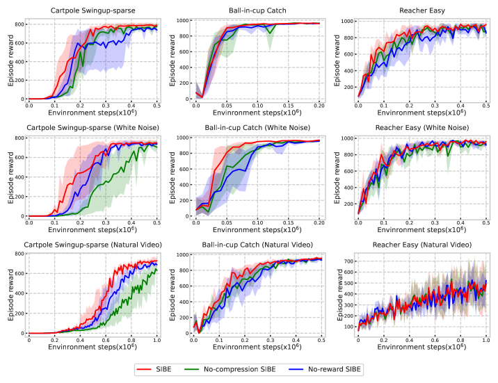
We show the performance of SIBE, Non-reward SIBE and Non-compression SIBE on three reward-sparse tasks in three settings in Fig. 10. SIBE achieves better or at least comparable performance to its own ablations across all tasks.
In Fig. 11 we present the performance of SIBE with 4 different chunk lengths on three reward-sparse tasks. Using at least two consecutive transitions achieves better performance than SIBE with chunk length on all three tasks.
