Foundations of the Wald Space for Phylogenetic Trees

Abstract.

Evolutionary relationships between species are represented by phylogenetic trees, but these relationships are subject to uncertainty due to the random nature of evolution. A geometry for the space of phylogenetic trees is necessary in order to properly quantify this uncertainty during the statistical analysis of collections of possible evolutionary trees inferred from biological data. Recently, the wald space has been introduced: a length space for trees which is a certain subset of the manifold of symmetric positive definite matrices. In this work, the wald space is introduced formally and its topology and structure is studied in detail. In particular, we show that wald space has the topology of a disjoint union of open cubes, it is contractible, and by careful characterization of cube boundaries, we demonstrate that wald space is a Whitney stratified space of type (A). Imposing the metric induced by the affine invariant metric on symmetric positive definite matrices, we prove that wald space is a geodesic Riemann stratified space. A new numerical method is proposed and investigated for construction of geodesics, computation of Fréchet means and calculation of curvature in wald space. This work is intended to serve as a mathematical foundation for further geometric and statistical research on this space.

1. Introduction

1.1. Background

Over billions of years, evolution has been driven by unobserved random processes. Inferences about evolutionary history, which by necessity are largely based on observations of present-day species, are therefore always subject to some level of uncertainty. Phylogenetic trees are used to represent possible evolutionary histories relating a set of species, or taxa, which form the leaves of each tree. Internal vertices on phylogenetic trees usually represent speciation events, and edge lengths represent the degree of evolutionary divergence over any given edge. Trees are typically inferred from genetic sequence data from extant species, and a variety of well-established statistical methods exist for phylogenetic inference (Felsenstein, 2003). These generally output a sample of trees – a collection of possible evolutionary histories compatible with the data. Moreover, evolutionary relationships can vary stochastically from one gene to another, giving a further source of random variation in samples of trees (Maddison, 1997). It is then natural to pose statistical questions about such samples: for example identifying a sample mean, identifying principal modes of variation in the sample, or testing differences between samples. This, in turn, calls for the design of suitable metric spaces in which each element is a phylogenetic tree on some fixed set of taxa, and which are ideally both biologically substantive and computationally tractable.

The design of these tree spaces is aggravated by the continuous and combinatorial nature of phylogenetic trees and furthermore, a metric space that is also a geodesic space (so that distance corresponds to the length of shortest paths, also called geodesics) is to be preferred, as it facilitates computation of statistics like the Fréchet mean significantly. The first geodesic space of phylogenetic trees was introduced by Billera et al. (2001) and is called the BHV space, where BHV is an acronym of the authors Billera, Holmes and Vogtmann. For a fixed set of species $L=\{1,\dots,N\}$, also called taxa or labels, with $3\leq N\in\mathbb{N}$, BHV space is constructed via embedding all phylogenetic trees into a Euclidean space $\mathbb{R}^{M}$, where $M\in\mathbb{N}$ is exponentially growing in $N$, and then taking the infinitesimally induced intrinsic distance on this embedded subset, giving a metric space. As a result, BHV space features a very rich and computationally tractable geometry as it is CAT(0) space, i.e. globally of non-positive curvature, and thus having unique geodesics and Fréchet means. Starting with the development of a polynomial time algorithm for computing geodesics and thereby overcoming the combinatorial difficulties (Owen and Provan (2011)), many algorithms have been derived for computing statistics like sample means (Bačák (2014); Miller et al. (2015)) and variance (Brown and Owen (2020)), confidence regions for the population mean (Willis (2016)) and principal component analysis Nye (2011, 2014); Nye et al. (2016), Feragen et al. 2013). The BHV paper has had considerable influence more widely on research in phylogenetics (see Suchard (2005) for example), non-Euclidean statistics (Marron and Alonso (2014)), algebraic geometry (Ardila and Klivans (2006)), probability theory (Evans et al. (2006)) and other area of mathematics (Baez and Otter (2015)). In addition to the BHV tree space, a variety of alternative tree spaces have been proposed, both for discrete and continuous underlying point sets of trees. For example, in the tropical tree space (Speyer and Sturmfels, 2004; Monod et al., 2022) edge weights are times, not evolutionary divergence, thus allowing for a distance metric between two trees involving tropical algebra.

The geometries of the BHV and tropical tree spaces are unrelated to the methods used to infer phylogenies from sequence data. In contrast, there are substantially different tree spaces that originate via the evolutionary genetic substitution models used by molecular phylogenetic methods for tree inference (see Yang (2006) for details of these). Evolutionary substitution models are essentially Markov processes on a phylogenetic tree with state space $\Omega$. For DNA sequence data, the state space is $\Omega=\{\mathrm{A},\mathrm{C},\mathrm{T},\mathrm{G}\}$. Under an appropriate set of assumptions on the substitution model, each tree determines a probability distribution on the set of possible letter patterns at the labelled vertices $L$, (i.e. a probability mass function $p\colon\Omega^{N}\to[0,1]$), $N=|L|$, and this can be used to compute the likelhiood of any tree. At about the same that BHV space was introduced, Kim (2000) provided a geometrical interpretation of tree estimation methods, where, given the substitution model, an embedding of phylogenetic trees into an $|\Omega|^{N}$-dimensional simplex using the likelihoods was discussed informally. The concept was then picked up by Moulton and Steel (2004), introducing the topological space known as the edge-product space, taking not only into account phylogenetic trees but also forests, characterising each forest via a vector containing correlations between all pairs of labels in $L$ under the induced distribution $p$. This representation is then an embedding of all phylogenetic forests into a $N(N-1)/2$-dimensional space. Using the same characterisation of phylogenetic trees via distributions on $\Omega^{N}$ obtained from a fixed substitution model, Garba et al. (2018) considered probabilistic distances to obtain metrics on tree space, but these metrics do not yield length spaces. Therefore, in Garba et al. (2021), the fact that all phylogenetic trees with a fixed fully resolved tree topology are a manifold was used to apply the Fisher information geometry for statistical manifolds on each such piece of the space to eventually obtain a metric space that is a length space. Additionally, instead of using substitution models with finite state space $\Omega$, Garba et al. (2021) considered a Gaussian model with state space $\Omega=\mathbb{R}$ in order to deal with the problem of computational tractability. The distributions characterising phylogenetic trees are then zero-mean multivariate Gaussians, and sums over $\Omega^{N}$ for discrete $\Omega$ are replaced with integrals over $\mathbb{R}^{N}$. The characterisation with this Gaussian model together with the choice of the Fisher information geometry and the extension to phylogenetic forests ultimately leads to the wald space, which is essentially an embedding of the phylogenetic forests into the real symmetric $N\times N$-dimensional strictly positive definite matrices $\mathcal{P}$ (Garba et al. (2021)). The elements of wald space are called wälder (“Wald” is a German word meaning “forest”).

Figure 1. Two trees $T_{1}$ and $T_{2}$ with positive edge length $\ell\in(0,\infty)$. Letting $\ell\to\infty$, the intuitive limit element for both trees is the forest $F$, as species are considered not related if their evolutionary distance approaches infinity. In wald space, the distance between $T_{1}$ and $T_{2}$ goes to zero accordingly as $\ell\to\infty$ and their limit is the forest $F$ that is also contained in wald space. In BHV space however, their distance goes to infinity as $\ell\to\infty$ and $F$ is not an element of the space.

The geometry of wald space is fundamentally different from BHV space (Garba et al. (2021); Lueg et al. (2021)), as illustrated in Fig. 1, which also underlines the biological reasonability of the wald space. Loosely speaking, wald space can be viewed topologically as being obtained by compactifying the boundaries at the “infinities” of BHV space, which comes with the price of fundamentally changing the geometry that is not locally Euclidean anymore. We avoid, though, the compactification at the “zeroes” of the edge-product space proposed by Moulton and Steel (2004) which suggests itself by mathematical elegance. It is biologically questionable, however, as it would allow different taxa to agree with one another. In Garba et al. (2021), apart from defining the wald space, certain properties of the space were established, such as showing the distance between any two points to be finite, and algorithms for approximating geodesics were proposed. In Lueg et al. (2021), a compact definition of wald space as well as more refined algorithms for approximating geodesics were introduced.

1.2. Contribution of this paper

Previous work on wald space established the space as a length space, and this paper was originally motivated by the aim of proving the existence of a minimising geodesic betweeen every two points, i.e. establishing wald space as a geodesic metric space, since the existence of geodesics is crucial for performing statistical analysis within the space. This aim is achieved in Theorem 4.2.1 below. The proof involves three essential characterisations of the elements of wald space (as graph-theoretic forests; as split systems; and as certain symmetric positive definite matrices). In turn, these enable a rigorous analysis of the topology of wald space, such as Theorem 3.3.5 about its stratified structure, in addition to providing a foundation for further research on this space.

The remainder of the paper is structured as follows. In Section 2 we define the wald space $\mathcal{W}$ for a fixed set of labels $\{1,\dots,N\}$ as equivalence classes of partially labelled graph-theoretic forests. The topology on $\mathcal{W}$ is obtained by defining a map $\psi$ from $\mathcal{W}$ into the set of $N\times N$ symmetric positive definite matrices and requiring $\psi$ to be a homeomorphism onto its image. We then provide an equivalent, but more tractable, definition in terms of splits or biparitions of labels, and an equivalent map $\phi$ from split-representations of wälder to symmetric positive definite matrices. In particular, we show that wald space can be identified topologically with a disjoint union of open unit cubes. Each open unit cube is called a grove. In Section 3 we describe the structure or stratification of the wald space by investigating on how the groves are glued together along their respective boundaries. This is achieved by first providing in Section 3.1 a detailed characterization of the matrices in the image $\phi(\mathcal{W})$ in terms of a set of algebraic constraints on the matrix elements. Using this characterization, for example, we show that wald space is contractible. Then in Section 3.2 we use a partial ordering of forest topologies, first introduced by Moulton and Steel (2004) to establish results about the boundaries of groves and the stratification of wald space. This culminates in Section 3.3 in which we prove wald space satifies certain axioms at grove boundaries, collectively known as Whitney condition (A) (Pflaum, 2001), which ensure that tangent spaces behave well as the boundaries of strata are approached. We then go on to consider the induced affine invariant or information geometry on wald space in Section 4. We show the topology induced by the metric is the same as the previous topology defined using $\phi$, and hence show that $\mathcal{W}$ is a geodesic metric space (i.e. every two points are connected by a minimising geodesic). Finally in Section 5, we use a new algorithm for computing approximate geodesics to explore the geometry on wald space, specifically computing sectional curvatures within groves and Alexandrov curvatures for fundamental examples. We also investigate the behaviour of the sample Fréchet mean, in particular with reference to the issue of stickiness observed in in BHV space (see for example Hotz et al. (2013); Huckemann et al. (2015) for a discription). In Section 6 we discuss the contributions of the paper and some of the many open questions and unsolved problems about the geometry of wald space.

1.3. Notation

Throughout the paper we use the following notation and concepts, where points 4–6 below can be found in standard textbooks of differential geometry, e.g. (Lang, 1999, Chapter XII):

1. $2\leq N\in\mathbb{N}$ is a fixed integer defining the set of labels $L=\{1,\dots,N\}$.

2. $\sqcup_{i=1}^{n}A_{i}$ denotes the union if the $A_{i}$ are pairwise disjoint ($i=1,\ldots,n$).

3. When we speak of partitions, no empty sets are allowed.

4. For a set $E$, its cardinality is denoted by $|E|$.

5. $\mathcal{S}$ is the Euclidean space of real symmetric $N\times N$ matrices.

6. $\mathcal{P}$ is the space of real symmetric and positive definite $N\times N$ matrices. It is an open cone in $\mathcal{S}$ and carries the topology and smooth manifold structure inherited from $\mathcal{S}$. In particular, every tangent space $T_{P}\mathcal{P}$ at $P\in\mathcal{P}$ is isomorphic to $\mathcal{S}$.

7. We equip $\mathcal{P}$ with the affine invariant Riemannian metric, also called information geometry, yielding a Cartan-Hadamard manifold. Its metric tensor is given by

   $$\langle X,Y\rangle_{P}=\operatorname*{trace}(P^{-1}XP^{-1}Y)$$

   for $X,Y\in\mathcal{S}\cong T_{P}\mathcal{P}$ and the unique geodesic $\gamma$ through $P=\gamma(0),Q=\gamma(1)\in\mathcal{P}$ is given by

   $$(-\infty,\infty)\to\mathcal{P},~{}t\mapsto\gamma(t)=\sqrt{P}\exp\left(t\log\left(\sqrt{P}^{-1}Q\sqrt{P}^{-1}\right)\right)\sqrt{P}$$

   with the usual matrix exponential and logarithm, respectively. Here, $\sqrt{P}$ denotes the unique positive definite root of $P$.

8. The Riemannian metric induces a metric on $\mathcal{P}$ denoted by $d_{\mathcal{P}}$ and for a rectifiable curve $\gamma:[a,b]\to\mathcal{P}$ let $L_{\mathcal{P}}(\gamma)$ be its length.

In a word of caution we note that the term topology appears in two contexts: (i) as a system of open sets defining a topological space and (ii) as a branching structure of a graph-theoretic forest. The latter is standard in the phylogenetic literature, despite the potential for confusion.

2. Definition of Wald Space via Graphs and Splits

2.1. From a Graph Viewpoint

This section recalls definitions and results from Garba et al. (2021) and Lueg et al. (2021).

Definition 2.1.1.

A forest is a triple $(\mathfrak{V},\mathfrak{E},\ell)$, where

1. $(\mathfrak{V},\mathfrak{E})$ is a graph-theoretical undirected forest with vertex set $\mathfrak{V}$ such that $L\subseteq\mathfrak{V}$ and that $v\in\mathfrak{V}\setminus L$ implies $\deg(v)\geq 3$, where $\deg(v)$ is the degree of a vertex $v$, and edge set $\mathfrak{E}\subseteq\big{\{}\{u,v\}:u,v\in\mathfrak{V},\,u\neq v\big{\}}$,

2. and $\ell=(\ell_{e})_{e\in\mathfrak{E}}\in(0,\infty)^{\mathfrak{E}}$.

Definition 2.1.2.

Two forests $(\mathfrak{V},\mathfrak{E},\ell),(\mathfrak{V}^{\prime},\mathfrak{E}^{\prime},\ell^{\prime})$ are topologically equivalent, if there is a bijection $f\colon\mathfrak{V}\to\mathfrak{V}^{\prime}$ such that

1. $f(u)=u$ for all $u\in L$,

2. $\{u,v\}\in\mathfrak{E}\Leftrightarrow\{f(u),f(v)\}\in\mathfrak{E}^{\prime}$.

They are phylogenetically equivalent if additionally

1. $\ell_{\{u,v\}}=\ell^{\prime}_{\{f(u),f(v)\}}$ for all edges $\{u,v\}\in\mathfrak{E}$.
   

Moreover,

1. Every phylogenetic equivalence class is called a phylogenetic forest and denoted by $\mathfrak{F}=[\mathfrak{V},\mathfrak{E},\ell]$.

2. $\mathcal{W}$ is the set of all phylogenetic forests.

3. Every topological equivalence class is called a forest topology and denoted by $[\mathfrak{F}]=[\mathfrak{V},\mathfrak{E}]$.

Definition 2.1.3.

Let $(\mathfrak{V},\mathfrak{E},\ell)$ be a forest. For two leaves $u,v\in L$ let $\mathfrak{E}(u,v)$ be the set of edges in $\mathfrak{E}$ of the unique path between $u$ and $v$, if $u$ and $v$ are connected, else set $\mathfrak{E}(u,v)=\emptyset$. Further define a mapping of forests via

$$\psi:(\mathfrak{V},\mathfrak{E},\ell)\mapsto\big{(}\rho_{uv}\big{)}_{u,v=1}^{N}\in\mathcal{S}$$

where

(2.1) $$\rho_{uv}=\left\{\begin{array}[]{cl}\displaystyle\exp\bigg{(}-\sum_{e\in\mathfrak{E}(u,v)}\ell_{e}\bigg{)}&\mbox{ if }u\neq v\mbox{ and }\mathfrak{E}(u,v)\neq\emptyset\\[10.00002pt] 0&\mbox{ if }u\neq v\mbox{ and }\mathfrak{E}(u,v)=\emptyset\\[10.00002pt] 1&\mbox{ if }u=v\end{array}\right.$$

for $1\leq u,v\leq N$.

By definition, the above matrix is the same for two forests representing the same phylogenetic forest. It is even positive definite and characterizes phylogenetic forests uniquely as the following theorem shows.

Theorem 2.1.4 (Garba et al. (2021), Theorem 4.1).

For every forest $(\mathfrak{V},\mathfrak{E},\ell)$, we have

$$\psi(\mathfrak{V},\mathfrak{E},\ell)\in\mathcal{P}$$

and for any two forests $(\mathfrak{V},\mathfrak{E},\ell)$ and $(\mathfrak{V}^{\prime},\mathfrak{E}^{\prime},\ell^{\prime})$ we have

$$\psi(\mathfrak{V},\mathfrak{E},\ell)=\psi(\mathfrak{V}^{\prime},\mathfrak{E}^{\prime},\ell^{\prime})$$

if and only if

$$[\mathfrak{V},\mathfrak{E},\ell]=[\mathfrak{V}^{\prime},\mathfrak{E}^{\prime},\ell^{\prime}]\,.$$

In consequence of Theorem 2.1.4, $\psi$ induces a well defined injection from $\mathcal{W}$ into $\mathcal{P}$. In slight abuse of notation we denote this mapping also by $\psi$, that is

(2.2) $$\psi\colon\mathcal{W}\to\mathcal{P},\quad\mathfrak{F}=[\mathfrak{V},\mathfrak{E},\ell]\mapsto\psi(\mathfrak{F})\coloneqq\psi(\mathfrak{V},\mathfrak{E},\ell).$$

Definition 2.1.5.

The wald space is the topological space $\mathcal{W}$ equipped with the unique topology under which the map $\psi\colon\mathcal{W}\to\mathcal{P}$ from Equation 2.2 is a homeomorphism onto its image.

2.2. From a Split Viewpoint

If $(\mathfrak{V},\mathfrak{E},\ell)$ is a representative of a phylogenetic forest $\mathfrak{F}$, there is $K\in\mathbb{N}$ such that the graph-theoretic forest $(\mathfrak{V},\mathfrak{E})$ decomposes into $K$ disjoint nonempty graph-theoretic trees

$$(\mathfrak{V}_{1},\mathfrak{E}_{1}),\ldots,(\mathfrak{V}_{K},\mathfrak{E}_{K})\,.$$

In particular, this decomposition induces a partition $L_{1},\ldots,L_{K}$ of the leaf set $L$ with $L_{\alpha}\subseteq\mathfrak{V}_{\alpha}$, $1\leq\alpha\leq K$.

Furthermore for $1\leq\alpha\leq K$, taking away an edge $e\in\mathfrak{E}_{\alpha}$ decomposes $(\mathfrak{V}_{\alpha},\mathfrak{E}_{\alpha})$ into two disjoint graph-theoretic trees that split the leaf set $L_{\alpha}$ into two disjoint subsets $A$ and $B$.

The representation of phylogenetic trees via splits is more abstract than as graphs but more tractable. We first introduce the weighted split representation and then show equivalence of the concepts.

Definition 2.2.1.

A tuple $F=(E,\lambda)$ with $E\neq\emptyset$ is a split-based phylogenetic forest if

1. there is $1\leq K\leq N$ and a partition $L_{1},\ldots,L_{K}$ of the leaf set $L$;

2. every element $e\in E$ is of the form $e=\{A,B\}$, called a split, where for some $1\leq\alpha\leq K$, $A,B$ is a partition of $L_{\alpha}$; $E_{\alpha}$ denotes the elements in $E$ that are splits of $L_{\alpha}$; for notational ease we write interchangeably

   $$e=\{A,B\}=A|B=a_{1}\ldots a_{r}|b_{1}\ldots b_{s}=a_{1}\ldots a_{r}|B=A|b_{1}\ldots b_{s}\,,$$

   whenever $A=\{a_{1},\ldots,a_{r}\}$, $B=\{b_{1},\ldots,b_{s}\}$;

3. all splits in $E_{\alpha}$ ($1\leq\alpha\leq K$) are pairwise compatible with one another, where two splits $A|B$ and $C|D$ of $L_{\alpha}$ are compatible with one another if one of the sets below is empty:

   $$A\cap C,\quad A\cap D,\quad B\cap C,\quad B\cap D\,;$$

4. for all distinct $u,v\in L_{\alpha}$, $1\leq\alpha\leq K$, there exists a split $e=A|B\in E_{\alpha}$ such that $u\in A$ and $v\in B$;

5. $\lambda\coloneqq(\lambda_{e})_{e\in E}\in(0,1)^{E}$.

Moreover $F_{\infty}$ with $E=\emptyset$ and void array $\lambda$ is the completely disconnected split-based phylogenetic forest with leaf partion $\{1\},\ldots,\{N\}$.

The partition $L_{1},\ldots,L_{K}$ is not mentioned explicitly in the definition of a split-based phylogenetic forest $F=(E,\lambda)$ since it can be derived from $E$ via $\{L_{1},\dots,L_{\tilde{K}}\}\coloneqq\big{\{}A\cup B\colon A|B\in E\big{\}}$, where $\tilde{K}\leq K$, and for all $u\in L\setminus\bigcup_{\alpha=1}^{\tilde{K}}L_{\alpha}$, the singleton $\{u\}$ is added to the collection to obtain $L_{1},\dots,L_{K}$.

Theorem 2.2.2.

There is a one-to-one correspondence between split-based phylogenetic forests $F=(E,\lambda)$ from Definition 2.2.1 and phylogenetic forests $\mathfrak{F}=[\mathfrak{V},\mathfrak{E},\ell]$ from Definition 2.1.2 with $\ell$ and $\lambda$ related by

(2.3) $$\lambda_{s}\coloneqq 1-\exp\big{(}-\ell_{e}\big{)}\,.$$

with an arbitrary but fixed representative $(\mathfrak{V},\mathfrak{E},\ell)$. Furthermore, there is a one-to-one correspondence between compatible split sets $E$ from Definition 2.2.1 (i) - (iv), and phylogenetic forest topologies $[\mathfrak{V},\mathfrak{E}]$.

Proof.

Case I. Suppose $K=1$, i.e. $\mathfrak{F}$ comprises only one tree: We take recourse to (Semple and Steel, 2003, Theorem 3.1.4) who establish a one-to-one correspondence of compatible split sets $E$ from Definition 2.2.1 (i) - (iv), and phylogenetic forest topologies $[\mathfrak{V},\mathfrak{E}]$, in case these are taken from graph-theoretic trees. Indeed, our phylogenetic forest topologies correspond to isomorphic X-trees there (our $L$ is $X$ there and the labelling map from (Semple and Steel, 2003, Definition 2.1.1) is the identity in our case) and for every representative $(\mathfrak{V},\mathfrak{E})\in[\mathfrak{V},\mathfrak{E}]$ there is a unique compatible split set $E$ from Definition 2.2.1 (i) - (iv) ((iv). is a consequence of $L\subseteq\mathfrak{V}$, $K=1$ and injectivity of the labelling map). Vice versa, there is a bijection $e\mapsto s_{e},\mathfrak{E}\to E$ that, removing the edge $e$ from $\mathfrak{E}$ produces two disconnected trees, yields a unique split $s=s_{e}=A|B$ of the leaf set $L=A\cup B$. This yields the second assertion, namely a one-to-one correspondence between compatible split sets $E$ from Definition 2.2.1 (i) - (iv) and phylogenetic forest topologies $[\mathfrak{V},\mathfrak{E}]$ in case of underlying graph-theoretic trees. The first assertion follows from the correspondence in (2.3), which thus yields, due to phylogenetic equivalence in Definition 2.1.2 (iii), a one-to-one correspondence between split based phylogenetic forests $F=(E,\lambda)$ and phylogenetic forests $[\mathfrak{V},\mathfrak{E},\ell]$, in case of underlying graph-theoretic trees.

Case II. Suppose $\mathfrak{F}$ comprises several $K>1$ trees: Here, consider two phylogenetic forests representatives $(\mathfrak{V},\mathfrak{E},\ell),(\mathfrak{V}^{\prime},\mathfrak{E}^{\prime},\ell^{\prime})\in[\mathfrak{V},\mathfrak{E},\ell]$. Due to Definition 2.1.2, (i) and (ii), both $(\mathfrak{V},\mathfrak{E},\ell)$ and $(\mathfrak{V}^{\prime},\mathfrak{E}^{\prime},\ell^{\prime})$ have the same number of connected components, each of which is a graph-theoretic tree and the bijection $f$ from Definition 2.1.2 restricts to bijections between the corresponding graph-theoretic trees. For each of these, Case I ($K=1$) is applicable, thus yielding the assertion in the general case. ∎

In consequence of Theorem 2.2.2 we introduce the following additional notation.

Definition 2.2.3.

From now on, we identify split-based phylogenetic forests $F=(E,\lambda)$ with phylogenetic forests $\mathfrak{F}=[\mathfrak{V},\mathfrak{E},\ell]$ and say that $F$ is a wald, in plural wälder, so that $F\in\mathcal{W}$, and use interchangeably the name split and edges for the elements of $E$ (as they are “edges” in equivalence classes). In particular, the $\lambda_{e},e\in E$, from Definition 2.2.1, 5., are called edge weights. Furthermore,

1. $[F]\coloneqq E$ also denotes the topology $[\mathfrak{V},\mathfrak{E}]$ of $F$ and

   $$\mathcal{E}:=\{E:\exists\lambda\in(0,1)^{E}\mbox{ such that }(E,\lambda)\mbox{ is a split-based phylogenetic forest}\}\cup\{\emptyset\}\,$$

   denotes the set of all possible topologies;

2. wälder of the same topology $E$ form a grove

   $$\mathcal{G}_{E}=\big{\{}F=(E^{\prime},\lambda^{\prime})\in\mathcal{W}\colon E=E^{\prime}\big{\}},$$

3. for any two $u,v\in L$ with leaf partition $L_{1},\ldots,L_{K}$, define

   $$E(u,v):=\{A|B:\exists\,1\leq\alpha\leq K\mbox{ and }e\in\mathfrak{E}(u,v)\mbox{ that splits }L_{\alpha}\mbox{ into }A\mbox{ and }B\}\,,$$

   which also denotes set of edges between $u$ and $v$, that may be empty;

4. the edge length based matrix representation $\psi$ from Equation 2.2 translates to the edge weight based matrix representation $\phi$ defined by

   (2.4) $$\phi\colon\mathcal{W}\to\mathcal{P},\quad F=(E,\lambda)\mapsto(\rho_{uv})_{u,v=1}^{N}\coloneqq\bigg{(}\prod_{e\in E(u,v)}\big{(}1-\lambda_{e}\big{)}\bigg{)}_{u,v=1}^{N},$$

   with the agreement that in case of empty $E(u,v)$

   (2.7) $$\left.\begin{array}[]{rl}&\rho_{uv}\coloneqq 1\text{ whenever }u=v\text{ and }\\ &\rho_{uv}\coloneqq 0\text{ whenever }u\in L_{\alpha}\text{ and }v\in L_{\beta}\text{, }\alpha\neq\beta\text{, }\alpha,\beta\in\{1,\dots,K\}\end{array}\right\}\,;$$

   here $\lambda$ is computed from $\ell$ as defined in Equation 2.3.

Remark 2.2.4.

In light of Definition 2.1.5, the wald space is the topological space $\mathcal{W}$ equipped with the unique topology such that the map $\phi\colon\mathcal{W}\to\mathcal{P}$ is a homeomorphism onto its image. Thus, groves can be identified topologically with open unit cubes

(2.8) $$\mathcal{G}_{E}\cong(0,1)^{E}\,$$

and the wald space thus with the disjoint union

(2.9) $$\mathcal{W}=\bigsqcup_{E\in\mathcal{E}}\mathcal{G}_{E}\cong\bigsqcup_{E\in\mathcal{E}}(0,1)^{E}\,,$$

where we note that $|E|$ runs from $0$ (corresponding to $F_{\infty}$) to $2N-3$ (for fully resolved trees), as is easily seen upon induction on $N$.

Furthermore, observe that

1. Equation 2.3 links strictly monotonous edge weights with edge lengths so that the limits $\lambda_{e}\to 0,1$ correspond to the limits $\ell_{e}\to 0,+\infty$, respectively;

2. for any partition $A,B$ of $L_{\alpha}$ ($1\leq\alpha\leq K$, as above), we have that

   (2.10) $$e=A|B\iff e\in E(u,v)\mbox{ for all }u\in A,v\in B\,,$$

   where the implication to the right is a consequence of $E_{\alpha}$ being a tree topology and the reverse implication is a consequence of $A$ and $B$ being a partition of $L_{\alpha}$.

Example 2.2.5.

Let $N=6$. Consider

$$E=\big{\{}1|234,3|124,4|123,12|34,5|6\big{\}},$$

i.e. the partition of labels is $L_{1}=\{1,2,3,4\}$, $L_{2}=\{5,6\}$, the corresponding graph is depicted in Figure 2. One can easily check that all edges that are splits of $L_{1}$ are compatible, likewise for all splits of $L_{2}$ (there is only one split, $5|6$, in this case).

Moreover, observe that the unique path from $1$ to $4$ contains the edges $E(1,4)=\big{\{}1|234,4|123,12|34\big{\}}$, i.e. all splits separating $1$ and $4$.

Indeed, for every connected pair of leaves, there is a split separating this pair, for instance for all $u,v\in L_{1}$ there is a split $e=A|B\in E$ such that $u\in A$ and $v\in B$. Removing the edge $1|234$ from the subtree comprising the leaf set $L_{1}$ violates this condition: If there is no split separating $1$ and $2$, which remain connected, then one vertex is labelled twice with $1$ and $2$. (Semple and Steel, 2003, e.g. Section 3.1.) allow such trees, we, however, exclude them.

Figure 2. The topology $E$ as defined in Example 2.2.5 with the corresponding splits annotated to the edges.

3. Topology and Stratification of Wald Space

3.1. Embedding

Recall from Theorem 2.1.4 that $\psi:\mathcal{W}\to\mathcal{P}$ from Equation 2.1 is injective and so is the equivalent $\phi:\mathcal{W}\to\mathcal{P}$ from Equation 2.4. Its image is characterized by algebraic equalities and inequalities, as shown by the the following theorem. Further exploration will yield that the topology of wald space is that of a stratified union of disjoint open unit cubes, each corresponding to a grove from Definition 2.2.3.

Theorem 3.1.1.

A matrix $P=(\rho_{uv})_{u,v=1}^{N}\in\mathcal{P}$ is the $\phi$-image of a wald $F\in\mathcal{W}$ if and only if all of the following conditions are satisfied for arbitrary $u,v,s,t\in L$:

1. $\rho_{uu}=1$,

2. two of the following three are equal and smaller than (or equal to) the third

   $$\rho_{uv}\rho_{st},\quad\rho_{us}\rho_{vt},\quad\rho_{ut}\rho_{vs}\,,$$

3. $\rho_{uv}\geq 0$.

Furthermore, the wald $F\in\mathcal{W}$ is then uniquely determined.

Before proving Theorem 3.1.1, we elaborate on the above algebraic conditions.

Remark 3.1.2.

1. Condition (R2) above is called the four-point-condition. In its non-strict version, all three products are equal and this indicates some degeneracy, namely that some internal vertices have degree four or higher. The four-point-condition is equivalent to (e.g. Buneman (1974) or (Semple and Steel, 2003, p.147))

   (3.1) $$\rho_{uv}\rho_{st}\geq\min\big{\{}\rho_{us}\rho_{vt},\;\rho_{ut}\rho_{vs}\big{\}}$$

   and implies (e.g. setting $s=t$ in (R2) and exploiting (R1))

   1. $\rho_{uv}\geq\rho_{us}\rho_{sv}$ for all $u,v,s\in L$.

   Notably (R1) and (R2) imply, in conjunction with $P\in\mathcal{P}$ that

   1. $\rho_{uv}<1$ for all $u\neq v$,

   for otherwise, if $\rho_{uv}=1$ for some $u\neq v$, Condition 1(R4) implied for any $s\in L$ that

   $$\rho_{us}\geq\rho_{uv}\rho_{vs}=\rho_{vs}\quad\text{ and }\quad\rho_{vs}\geq\rho_{uv}\rho_{us}=\rho_{us},$$

   so $\rho_{us}=\rho_{vs}$ and hence, $P$ would be singular, a contradiction to $P\in\mathcal{P}$.

2. Observe that $\phi(F)=(\exp(-d_{uv}))_{u,v=1}^{N}$, where the $d_{uv}$ are the finite or infinite distances

   $$d_{uv}\coloneqq\sum_{e\in E(u,v)}\ell_{e}=-\log\rho_{uv},$$

   between leaves $u,v\in L$, and, with Definition 2.2.3 5., this translates to $d_{uu}=0$ and $d_{uv}=\infty$ whenever $u$ and $v$ are in different components. In the literature, $(d_{uv})_{u,v=1}^{N}$ is also called tree metric (e.g. (Semple and Steel, 2003, Chapter 7)) or distance matrix (e.g. (Felsenstein, 2003, Chapter 11)). Indeed, it conveys a metric on $L$ as Condition 1(R4) encodes the triangle inequality (for any $u,v,s\in L$)

   $$d_{uv}\leq d_{us}+d_{vs}.$$

3. In particular, the unit $N\times N$ matrix $I=(\delta_{uv})_{u,v\in L}\in\mathcal{P}$ is the $\phi$-image of the complete disconnected wald $F_{\infty}\in\mathcal{W}$ with topology $E_{\infty}=\emptyset$ in which each leaf comprises one of the $K=N$ single element trees.

4. For a given $P\in\mathcal{P}$ satisfying conditions (R1), (R2) and (R3) there are neighbour joining algorithms in (Semple and Steel, 2003, Scn 7.3), determining its split $E\in\mathcal{E}$.

Proof of Theorem 3.1.1..

“$\Longrightarrow$”. Let $F\in\mathcal{W}$ and $(\rho_{uv})_{u,v=1}^{N}=\phi(F)$. (R1) and (R3) hold by definition. Further, applying Semple and Steel (2003, Theorem 7.2.6) to each connected component asserts (R2) for all $u,v,s,t\in L_{\alpha}$ for all $\alpha=1,\dots,K$. Furthermore, since $\rho_{uv}=0$ whenever $u\neq v$ are in different components, for any $s\in L\setminus\{u,v\}$, $\rho_{us}=0$ or $\rho_{vs}=0$, so (R2) holds true in general.

“$\Longleftarrow$”. Let $P=(\rho_{uv})_{u,v=1}^{N}\in\mathcal{P}$ satisfy (R1), (R2) and (R3) (and thus by Remark 3.1.2 also 1(R4) and 1(R5)). The equivalence relation on $L$, defined by $u\sim v\iff\rho_{uv}\neq 0$ partitions $L$ into $L_{1},\dots,L_{K}$ for some $K\in\{1,\dots,N\}$. For each $\alpha=1,\dots,K$, apply Semple and Steel (2003, Theorem 7.2.6) to each tree metric $(d_{uv})_{u,v\in L_{\alpha}}$ (defined in Remark 3.1.2 2.) to obtain a unique corresponding tree, say $[\mathfrak{V}_{\alpha},\mathfrak{E}_{\alpha},\ell^{(\alpha)}]$, where, in contrast to our definition, Semple and Steel (2003) allow leaves on top of each other, in their language, vertices labelled more than once. The union of trees gives a forest $\mathfrak{F}=[\mathfrak{V},\mathfrak{E},\ell]$ with label set $L$ with $\mathfrak{V}=\bigcup_{\alpha}\mathfrak{V}_{\alpha}$, $\mathfrak{E}=\bigcup_{\alpha}\mathfrak{E}_{\alpha}$, satisfying $\psi(\mathfrak{F})=P$. Suppose now a vertex was labelled more than once, say, with distinct leaf labels $u,v\in L_{\alpha}$, i.e. $u\neq v$, for some $\alpha=1,\dots,K$. Then, $u$ and $v$ have zero distance $d_{uv}$, hence $\rho_{uv}=1$, yielding a contradiction to 1(R5) (i.e. $P\not\in\mathcal{P}$ as argued in Remark 3.1.2 1.) Thus $\mathfrak{F}\in\mathcal{W}$ and with Definition 2.2.3, we obtain $F\in\mathcal{W}$ with $\phi(F)=\psi(\mathfrak{F})=P$. ∎

Since $\phi(\mathcal{W})$ is defined by algebraic equalities and nonstrict inequalities, we have the following corrollary at once.

Corollary 3.1.3.

$\phi(\mathcal{W})\subseteq\mathcal{P}$ is a closed subset of $\mathcal{P}$.

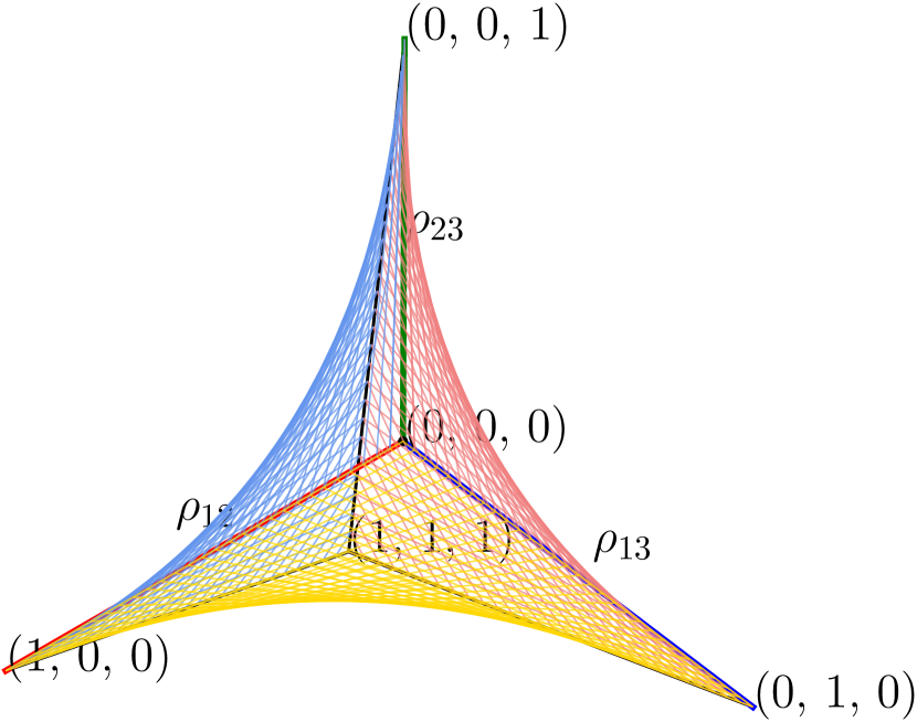
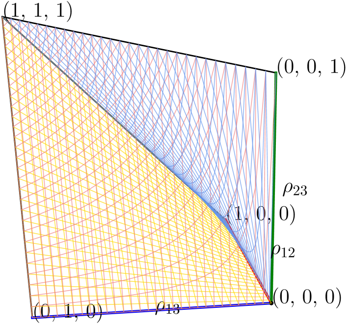
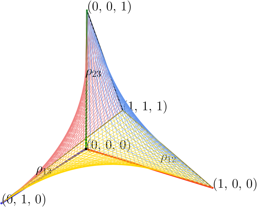
Example 3.1.4 ($\mathcal{W}$ for $N=3$).

For $N=3$, all matrices $P=\phi(F)$ with $F\in\mathcal{W}$ are given by (using Theorem 3.1.1)

$$\begin{pmatrix}1&\rho_{12}&\rho_{13}\\ \rho_{12}&1&\rho_{23}\\ \rho_{13}&\rho_{23}&1\end{pmatrix}\quad\text{satisfying the triangle inequalities}\quad\left\{\begin{array}[]{c}\rho_{12}\geq\rho_{13}\rho_{23},\\ \rho_{13}\geq\rho_{12}\rho_{23},\\ \rho_{23}\geq\rho_{12}\rho_{13},\end{array}\right.$$

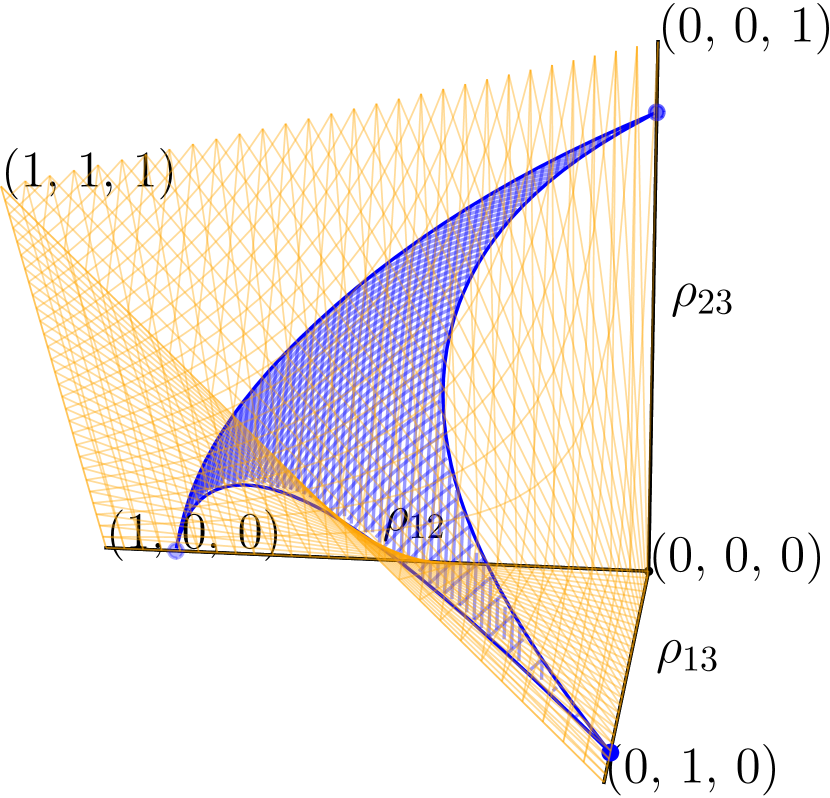
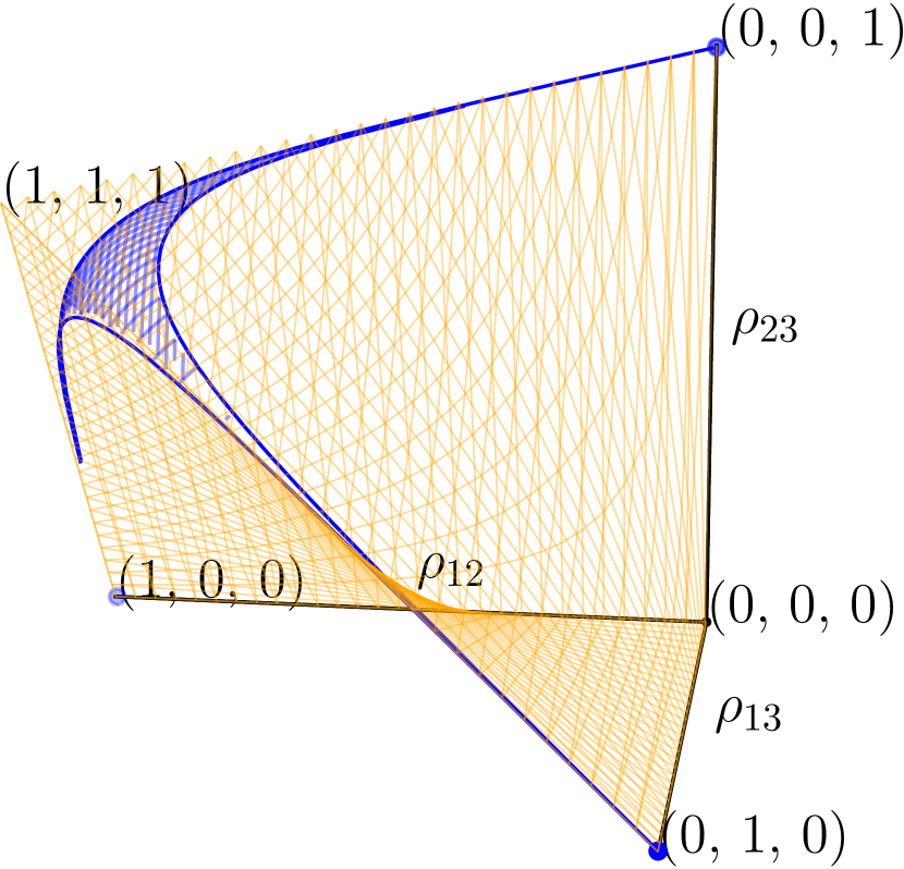
and $0\leq\rho_{12},\rho_{13},\rho_{23}<1$. This set in coordinates $\rho_{12},\rho_{13},\rho_{23}$ is depicted in Figure 3, where the two-dimensional surfaces correspond to the non-linear boundaries resulting from the triangle inequalities. Note that the regions, where at least one coordinate is one, are not included in $\phi(\mathcal{W})$, as the corresponding matrix is no longer strictly positive definite.

Figure 3. $\phi(\mathcal{W})$ for $N=3$ embedded in $\mathcal{P}$, where only the off-diagonal entries on the boundary are depicted. Note that the geometry of the wald space is not Euclidean and thus this depiction may be deceiving (as it is a non-isometric embedding into $\mathbb{R}^{3}$), e.g. the regions where one coordinate equals 1 are infinitely far away.

Corollary 3.1.5.

Conveyed by the homeomorphism $\phi$, $\mathcal{W}$ is star shaped as a subset $\mathbb{R}^{N\times N}$ with respect to $F_{\infty}$ and hence contractible.

Proof.

Let $F\in\mathcal{W}$ with $\phi(F)=P=(\rho_{uv})_{u,v\in L}$ satisfying (R1) - (R3) by Theorem 3.1.1. Recalling from Remark 3.1.2, 3., that $\phi(F_{\infty})=I$, consider

$$(\rho_{uv}^{(x)})_{u,v\in L}=P^{(x)}=x\,I+(1-x)P,$$

and observe that for all $x\in[0,1]$, $P^{(x)}\in\mathcal{P}$, $\rho^{(x)}_{uu}=1=\rho_{uu}$ for all $u\in L$ and $\rho^{(x)}_{uv}=(1-x)\rho_{uv}\geq 0$ for all $u,v\in L$ with $u\neq v$, i.e. $P^{(x)}$ satisfies (R1) and (R3) for all $x\in[0,1]$. Moreover, to see that $P^{(x)}$ satisfies Equation 3.1 for all $x\in(0,1)$ for all $u,v,s,t\in L$, assume w.l.o.g that

(3.2) $$\rho_{uv}\rho_{st} =\rho_{us}\rho_{vt}\leq\rho_{ut}\rho_{vs}\,.$$

If all four $u,v,s,t$ are pairwise distinct then

(3.3) $$\rho^{(x)}_{uv}\rho^{(x)}_{st} =\rho^{(x)}_{us}\rho^{(x)}_{vt}\leq\rho^{(x)}_{ut}\rho^{(x)}_{vs}\,,$$

as well. If only one pair is equal, there are two typical cases. If $u=v$, say, we obtain a different but valid four point condition

$$\rho^{(x)}_{uv}\rho^{(x)}_{st}~{}\geq~{}\rho^{(x)}_{us}\rho^{(x)}_{vt}~{}=~{}\rho^{(x)}_{ut}\rho^{(x)}_{vs}\,,$$

where the inequality is strict in case of $\rho_{st}>0$ due to $1-x>(1-x)^{2}$. If $u=t$, say, then we obtain Equation 3.3 where the inequality is strict if $\rho_{vs}>0$. If exactly two pairs are the same, then, with the above setup only $u=t$ and $v=s$ is possible and both Equation 3.2 and Equation 3.3 are strict. In case of three equal indices, one different, or the same, Equation 3.3 holds again. Therefore, $P^{(x)}$ satisfies (R2) for all $x\in[0,1]$, and by Theorem 3.1.1 the entire continuous path $x\mapsto P^{(x)},[0,1]\to\mathcal{P}$ corresponds to a path $F^{(x)}\coloneqq\phi^{-1}(P^{(x)})\in\mathcal{W}$, connecting $F=F^{(0)}$ with $F_{\infty}=F^{(1)}$ as asserted. ∎

Showing contractibility of the edge-product space, Moulton and Steel contract to the same forest (cf. (Moulton and Steel, 2004, Proposition 5.1)), employing a different proof, however.

Remark 3.1.6.

We make the following observations about the proof of Corollary 3.1.5.

1. All of the wälder $\phi^{-1}(P^{(x)})$, for $0\leq x<1$ in the proof share the same partition of leaves into connected tree components, due to $\rho_{uv}\neq 0\iff(1-x)\rho_{uv}\neq 0$ for all $x\in[0,1)$ for all $u,v\in L$.

2. For $0<x<1$, $P^{(x)}$ satisfies unchanged, strict or nonstrict four-point conditions (R2), that may be different, though, from those of $P^{(0)}=\phi(F)$.

3. All triangle inequalites 1(R4) involving initial nonzero $\rho_{uv}$ are strict, however, for $0<x<1$, so that for $\phi^{-1}(P^{(x)})$ none of the leaves have degree 2. For example, starting with the wald consisting of a chain of three vertices with $N=3$ (so each vertex is labelled and the middle is of degree two), it is immediately transformed into a fully resolved tree (and stays one for all $x\in(0,1)$).

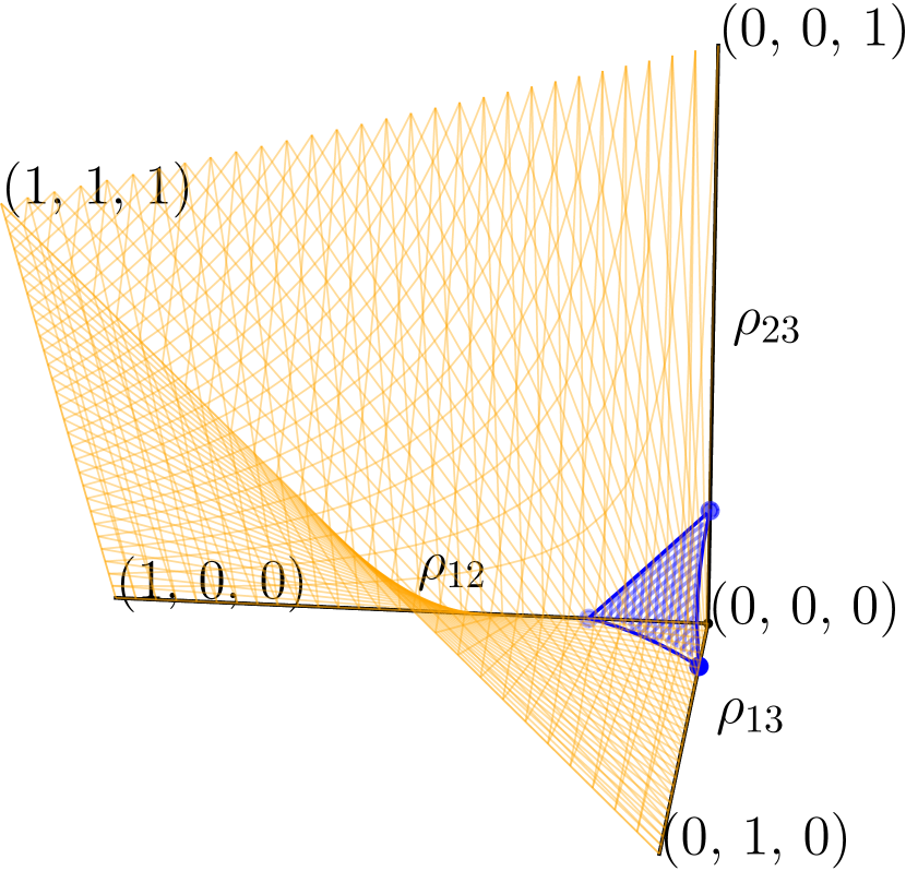
4. The point $F_{\infty}$ can be viewed as a vantage point of $\mathcal{W}$ which is then a bounded part of a cone where every

   $$B_{a}=\Big{\{}F\in\mathcal{W}\;\Big{|}\;\phi(F)=(\rho_{uv})_{u,v=1}^{N},~{}a=1-\prod_{\begin{subarray}{c}u,v=1\\ u<v\end{subarray}}^{N}\big{(}1-\rho_{uv}\big{)}\Big{\}}.$$

   is a slice of level $a\in[0,1)$. Then for every $F\in B_{a}$, there is $r_{F}>1$ such that

   $$F=\phi^{-1}\left((1-x)\phi(F_{\infty})+x\phi(F)\right)\in\mathcal{W}$$

   for all $0\leq x<r_{F}$ and $\phi(F)$ is singular for $x=r_{F}$. For $N=3$, the set $B_{a}$ for several $a\in(0,1]$ embedded into $\mathcal{P}$ is depicted in Fig. 4.

Figure 4. Depicting the off-diagonal matrix entries of $\phi(\mathcal{W})$ embedded in $\mathcal{P}$ for $N=3$ (orange boundary) in a 3-dimensional coordinate system (cf. Example 3.1.4) and the 2-dimensional images $\phi(B_{a})$ (purple) of the slices $B_{a}$ for $a=0.2,0.87,0.997$ (from left to right).

We next consider the restriction of the map $\phi$ to each grove $\mathcal{G}_{E}$ explicitly in terms of edge weights.

Definition 3.1.7.

With the agreement (2.7) in case of empty $E(u,v)$, we denote the restriction of $\phi\colon\mathcal{W}\to\mathcal{P}$ from Definition 2.2.3 to a grove $\mathcal{G}_{E}$ by

(3.4) $$\phi_{E}\colon(0,1)^{E}\to\mathcal{P},\qquad\lambda\mapsto(\rho_{uv})_{u,v\in L}=\Bigg{(}\prod_{e\in E(u,v)}\big{(}1-\lambda_{e}\big{)}\Bigg{)}_{u,v=1}^{N};$$

its continuation onto all of $\mathbb{R}^{E}$ is denoted by

(3.5) $$\bar{\phi}_{E}\colon\mathbb{R}^{E}\to\mathcal{S},\qquad\lambda\mapsto(\rho_{uv})_{u,v\in L}=\Bigg{(}\prod_{e\in E(u,v)}\big{(}1-\lambda_{e}\big{)}\Bigg{)}_{u,v=1}^{N},$$

Remark 3.1.8.

The continuation $\bar{\phi}_{E}$ is multivariate real analytic on all of $\mathbb{R}^{E}$.

The following theorem characterizes each grove.

Theorem 3.1.9.

1. For $F=(E,\lambda)\in\mathcal{W}$ with $\phi(F)=(\rho_{uv})_{u,v\in L}$ we have

   $$\lambda_{e}=1-\max_{\begin{subarray}{c}u,v\in A\\ s,t\in B\end{subarray}}\sqrt{\frac{\rho_{ut}\rho_{vs}}{\rho_{uv}\rho_{st}}}\,,\mbox{ for all }e=A|B\in E\,.$$

2. The derivative of $\phi_{E}$ has full rank $|E|$ throughout $(0,1)^{E}$.

3. The map $\phi_{E}\colon(0,1)^{E}\cong\mathcal{G}_{E}\to\mathcal{P}$ is a smooth embedding.

Proof.

For the first assertion consider $e=A|B$, where $A\cup B=L_{\alpha}$, for some $1\leq\alpha\leq K$ and where $L_{1},\ldots,L_{K}$ is the leaf partition induced by $E$. Then the matrix entries $d_{uv}\coloneqq-\log\,\rho_{uv}$ ($u,v\in L_{\alpha}$) define a metric on $L_{\alpha}$, as noted in Remark 3.1.2. For such a metric, (Buneman, 1971, Lemma 8) asserts that one can assign a tree $(\mathfrak{V}_{\alpha},\mathfrak{E}_{\alpha},\ell^{\alpha})$ where

(3.6) $$\ell^{\alpha}_{e}=\min_{\begin{subarray}{c}u,v\in A\\ s,t\in B\end{subarray}}\frac{1}{2}\big{(}d_{ut}+d_{vs}-d_{uv}-d_{st}\big{)},$$

which is uniquely determined by (Buneman, 1971, Theorem 2). Due to our uniqueness results from Theorem 2.2.2 and Theorem 3.1.1, due to Equation 2.3, $\lambda_{e}=1-\exp(-\ell^{\alpha}_{e})$ and hence, using $\rho_{uv}=\exp(-d_{uv})$, the asserted equation follows at once from Equation 3.6.

For the second assertion, let $e\in E$ and suppose that $F=(E,\lambda)$ decomposes into $K$ subtrees inducing the leaf partition $L_{1},\ldots,L_{K}$. Using Equation 3.4, if either $u,v\in L$ are in different subtrees or $u=v$, then

$$\bigg{(}\frac{\partial\phi_{E}}{\partial\lambda_{e}}(\lambda)\bigg{)}_{uv}=0\,.$$

Else, if $u,v\in L_{\alpha}$ for some $1\leq\alpha\leq K$, then $\rho_{uv}>0$ and with the Kronecker delta $\delta$,

(3.7) $$\bigg{(}\frac{\partial\phi_{E}}{\partial\lambda_{e}}(\lambda)\bigg{)}_{uv}=-\delta_{e\in E(u,v)}\prod_{\begin{subarray}{c}\tilde{e}\in E(u,v)\\ \tilde{e}\neq e\end{subarray}}\big{(}1-\lambda_{\tilde{e}}\big{)}=-\frac{\rho_{uv}}{1-\lambda_{e}}\delta_{e\in E(u,v)}\,,$$

Thus, for every $x\in\mathbb{R}^{E}$, we have

$$\Big{(}(\mathrm{d}\phi_{E})_{\lambda}(x)\Big{)}_{uv}=-\rho_{uv}\,\sum_{e\in E}\frac{x_{e}}{1-\lambda_{e}}\delta_{e\in E(u,v)}\,,$$

so that $\Big{(}(\mathrm{d}\phi_{E})_{\lambda}(x)\Big{)}_{uv}=0$ implies

(3.8) $$0=\sum_{e\in E(u,v)}\frac{x_{e}}{1-\lambda_{e}}\eqqcolon h_{uv}.$$

We now view each of the $\ell^{\prime}_{e}:=\frac{x_{e}}{1-\lambda_{e}}$, $e\in E$ as a real valued “length” of $e$. With a representative $(\mathfrak{V},\mathfrak{E})$ of $E$ with leaf set partition $L_{1},\ldots,L_{K}$, for every $e\in E$ there are $v_{1},v_{2}\in\mathfrak{V}_{\alpha}$ with suitable $1\leq\alpha\leq K$ such that $e$ corresponds to $\{v_{1},v_{2}\}\in\mathfrak{E}_{\alpha}$. In particular, since $(\mathfrak{V}_{\alpha},\mathfrak{E}_{\alpha})$ is a tree, there are $u,v,s,t\in L_{\alpha}$ (not necessarily all of them distinct), such that

$$\ell^{\prime}_{e}=\frac{1}{2}\big{(}h_{uv}+h_{st}-h_{ut}-h_{vs}\big{)}.$$

If the r.h.s. is zero due to Equation 3.8, then $x_{e}=0$, yielding that $(\mathrm{d}\phi_{E})_{\lambda}$ has full rank, as asserted.

The third assertion follows directly from 1. and 2., i.e. $\phi_{E}$ is bijectively smooth onto its image and its differential is injective. ∎

In the following, we are concerned with $\bar{\phi}_{E}(\lambda)$ if $\lambda\in(0,1)^{E}$ approaches the boundary. The next result characterises exactly under which conditions $\bar{\phi}_{E}(\lambda)$ stays in the image $\phi(\mathcal{W})$ of wald space under $\phi$.

Lemma 3.1.10.

Let $F\in\mathcal{W}$ with topology $[F]=E$ and let $\lambda^{*}\in\partial([0,1]^{E})$ with $\bar{\phi}_{E}(\lambda^{*})=(\rho_{uv}^{*})_{u,v=1}^{N}$. Then

$$\bar{\phi}_{E}(\lambda^{*})\in\phi(\mathcal{W})\iff\bar{\phi}_{E}(\lambda^{*})\in\mathcal{P}\iff\rho_{uv}^{*}<1\text{ for all }u,v\in L\text{ with }u\neq v.$$

Proof.

The first equivalence follows from that Equation 3.9 is well-defined. We prove the second equivalence.
“$\Rightarrow$”: Follows from Remark 3.1.2, Condition (R5).
“$\Leftarrow$”: Analogously to the proof of Theorem 3.1.1, “$\Leftarrow$”, we find a phylogenetic forest in the sense of (Semple and Steel, 2003, Chapter 2.8), whose tree metric coincides with the one obtained from $\bar{\phi}_{E}(\lambda^{*})$, but there might be multiply labelled vertices. However, this is impossible due to $\rho_{uv}^{*}<1$ for any $u\neq v$, which is equivalent to a distance greater than zero between $u$ and $v$. Therefore, there exists a phylogenetic forest $F^{\prime}\in\mathcal{W}$ with $\phi(F^{\prime})=\bar{\phi}_{E}(\lambda^{*})$, and thus by Theorem 3.1.1, $\bar{\phi}_{E}(\lambda^{*})\in\mathcal{P}$. ∎

The previous result immediately shows which matrices in $\mathcal{P}$ form the boundary of a grove.

Corollary 3.1.11.

Let $E$ be a wald topology. Then the boundary of the grove $\mathcal{G}_{E}$ in $\mathcal{W}$ is given by

(3.9) $$\partial\mathcal{G}_{E}=\Big{\{}\phi^{-1}\big{(}\bar{\phi}_{E}(\lambda^{*})\big{)}\colon\lambda^{*}\in\partial([0,1]^{E}),\;\bar{\phi}_{E}(\lambda^{*})\in\mathcal{P}\Big{\}}\,.$$

The following result gives a first glimpse on how different groves are connected through the convergence of wälder.

Theorem 3.1.12.

Let $\mathcal{W}\ni(E_{n},\lambda^{(n)})=F_{n}\to F^{\prime}=(E^{\prime},\lambda^{\prime})\in\mathcal{W}$. Then there is a subsequence $n_{k}$, $k\in\mathbb{N}$, and a common topology $E$ such that $E_{n_{k}}=E$ for all $k\in\mathbb{N}$. Furthermore

1. $\lambda^{(n_{k})}$ has a cluster point $\lambda^{*}\in[0,1]^{E}$,

2. and $\phi(F^{\prime})=\bar{\phi}_{E}(\lambda^{*})$ for every of such cluster point $\lambda^{*}\in[0,1]^{E}$,

3. and $F^{\prime}\in\partial\mathcal{G}_{E}$ whenever $E\neq E^{\prime}$.

Proof.

For the first assertion, noting that there are only finitely many wald topologies, there needs to exist a subsequence $F_{n_{k}}$ of $F_{n}$ with $E_{n_{k}}=E$ for some topology $E$ for all $k\in\mathbb{N}$, and thus, since $F_{n_{k}}\in\mathcal{G}_{E}\cong(0,1)^{E}$, there exists $\lambda^{(n_{k})}\in(0,1)^{E}$ with $\phi_{E}(\lambda^{(n_{k})})=\phi(F_{n_{k}})$ for all $k\in\mathbb{N}$.

For 1., by Bolzano-Weierstraß, there needs to exist a cluster point $\lambda^{*}\in[0,1]^{E}$ of $\lambda^{(n_{k})}$.

For 2., for any cluster point $\lambda^{*}\in[0,1]^{E}$, from the continuity of $\bar{\phi}_{E}$, $\bar{\phi}_{E}(\lambda^{*})$ is a cluster point of $(\phi(F_{n}))_{n\in\mathbb{N}}$ and by $F_{n}\to F^{\prime}$ we find $\phi(F_{n})\to\phi(F^{\prime})$ and thus $\bar{\phi}_{E}(\lambda^{*})=\phi(F^{\prime})$.

For 3., let $\lambda^{*}\in[0,1]^{E}$ be a cluster point. If $\lambda^{*}\in(0,1)^{E}$ then $F^{\prime}\in\mathcal{G}_{E}$ and $E=E^{\prime}$, a contradiction. Thus $\lambda^{*}\in\partial([0,1]^{E})$, and due to $\bar{\phi}_{E}(\lambda^{*})=\phi(F^{\prime})\in\mathcal{P}$, the assertion follows. ∎

The following example teaches that when $F_{n}\to F$, $\lambda^{(n)}$ can have distinct cluster points.

Example 3.1.13.

Let $N=3$, set $e_{i}\coloneqq u|(L\setminus\{u\})$, $u\in L=\{1,2,3\}$ and $E=\{e_{1},e_{2},e_{3}\}$. Define the sequence of wälder $F_{n}\coloneqq(E,\lambda^{(n)})$, $n\in\mathbb{N}$, using a sequence $\varepsilon_{n}\in(0,\frac{1}{4})$ with $\varepsilon_{n}\to 0$ as $n\to\infty$, via

$$\lambda^{(2n-1)}_{e_{1}}\coloneqq\frac{1}{2}-\varepsilon_{n}, \lambda^{(2n-1)}_{e_{2}}\coloneqq\varepsilon_{n}, \lambda^{(2n-1)}_{e_{3}}\coloneqq 1-\varepsilon_{n},$$

$$\lambda^{(2n)}_{e_{1}}\coloneqq\varepsilon_{n}, \lambda^{(2n)}_{e_{2}}\coloneqq\frac{1}{2}-\varepsilon_{n}, \lambda^{(2n)}_{e_{3}}\coloneqq 1-\varepsilon_{n}.$$

The corresponding forests are depicted in Figure 5. Clearly, the sequence $\lambda^{(n)}$ ($n\in\mathbb{N}$) has two distinct cluster points $(1/2,0,1),(0,1/2,1)\in(0,1)^{3}$. We observe, however, that

$$\phi(F_{2n-1})=\begin{pmatrix}1&(1-\varepsilon_{n})(\frac{1}{2}+\varepsilon_{n})&(\frac{1}{2}+\varepsilon_{n})\varepsilon_{n}\\ (1-\varepsilon_{n})(\frac{1}{2}+\varepsilon_{n})&1&(1-\varepsilon_{n})\varepsilon_{n}\\ (\frac{1}{2}+\varepsilon_{n})\varepsilon_{n}&(1-\varepsilon_{n})\varepsilon_{n}&1\end{pmatrix}\overset{n\to\infty}{\longrightarrow}\begin{pmatrix}1&\frac{1}{2}&0\\ \frac{1}{2}&1&0\\ 0&0&1\end{pmatrix},$$

and similarly, $\phi(F_{2n})$ converges to the same matrix as $n\to\infty$. Letting $e^{\prime}=1|2$ and defining $F^{\prime}=(E^{\prime},\lambda^{\prime})=(\{e^{\prime}\},\lambda^{\prime})$ with $\lambda^{\prime}_{e^{\prime}}=\frac{1}{2}$ (i.e. label partitions $L^{\prime}_{1}=\{3\}$, $L^{\prime}_{2}=\{1,2\}$; cf. Figure 5), we have that $\phi(F_{n})\to\phi(F^{\prime})$, so $F_{n}\to F^{\prime}$.

Figure 5. A sequence of wälder (left and middle) converging (right) but having different $\lambda$ cluster points as detailed in Example 3.1.13.

Theorem 3.1.12 shows that whenever a sequence of wälder $F_{n}\in\mathcal{G}_{E}$ converges to a wald $F^{\prime}\in\mathcal{W}$ with topology $E^{\prime}$ and $F^{\prime}\notin\mathcal{G}_{E}$, then $F^{\prime}\in\partial\mathcal{G}_{E}$. In the following section we make this relationship between $E^{\prime}$ and $E$ more precise and unravel the boundary correspondences via a partial ordering on the wald topologies.

3.2. At Grove’s End

In light of Theorem 3.1.12, we investigate how two wald topologies $E=[F]$ and $E^{\prime}=[F^{\prime}]$ are related to each other.

Definition 3.2.1.

Let $F\in\mathcal{W}$ be a wald with topology $E=[F]$. For an edge $e=A|B\in E$, we define the edge restricted to some subset $L^{\prime}\subseteq L$ by

$$e|_{L^{\prime}}\coloneqq(A\cap L^{\prime})|(B\cap L^{\prime})$$

if both of the sets above are non void, else, we say that the restriction does not exist. In case of existence, we also say that $e|_{L^{\prime}}$ is a valid split.

The following definition is from Moulton and Steel (2004) and translated into the language of wälder and their topologies.

Definition 3.2.2.

For two wälder $F,F^{\prime}\in\mathcal{W}$ with topologies $E=[F],E^{\prime}=[F^{\prime}]$, respectively, we say that

(3.10) $$E^{\prime}=[F^{\prime}]\leq[F]=E$$

if all of the following three properties hold:

Refinement:

with the partitions $L_{1},\dots,L_{K}$ and $L^{\prime}_{1},\ldots,L_{K^{\prime}}^{\prime}$ of $L$ induced by $E^{\prime}$ and $E$, respectively, for every $1\leq\alpha^{\prime}\leq K^{\prime}$ there is $1\leq\alpha\leq K$ with $L^{\prime}_{\alpha^{\prime}}\subseteq L_{\alpha}$;

Restriction:

for every $1\leq\alpha^{\prime}\leq K^{\prime}$,

$$E^{\prime}_{\alpha^{\prime}}\subseteq E|_{L^{\prime}_{\alpha^{\prime}}}\coloneqq\big{\{}\tilde{e}\colon\exists e\in E\mbox{ such that }\tilde{e}\coloneqq e|_{L^{\prime}_{\alpha^{\prime}}}\text{ is a valid split}\big{\}}$$

where the r.h.s. is the set of splits $E$ restricted to $L^{\prime}_{\alpha^{\prime}}$;

Cut:

for every $1\leq\alpha^{\prime}_{1}\neq\alpha^{\prime}_{2}\leq K^{\prime}$ and $1\leq\alpha\leq K$ with $L^{\prime}_{\alpha^{\prime}_{1}},L^{\prime}_{\alpha^{\prime}_{2}}\subset L_{\alpha}$, there is some

$$A|B\in E\mbox{ with }L^{\prime}_{\alpha^{\prime}_{1}}\subseteq A,~{}L^{\prime}_{\alpha^{\prime}_{2}}\subseteq B\,.$$

Further, we say $E^{\prime}<E$ if $E\neq E^{\prime}\leq E$. We also write $F^{\prime}<F$ if $E^{\prime}<E$.

The restriction condition above corresponds to the definition of a tree displaying another tree in Moulton and Steel (2004). From (Moulton and Steel, 2004, Lemma 3.1), it follows at once that the relation $\leq$ as defined in Equation 3.10 is a partial ordering.

Example 3.2.3.

Let $N=5$, so $L=\{1,\dots,5\}$. Define three wald topologies

$$E =\big{\{}1|2345,12|345,3|1245,123|45,1234|5,1235|4\big{\}},$$

$$E_{1}^{\prime} =\{2|3,4|5\},$$

$$E_{2}^{\prime} =\{2|5,3|4\big{\}}.$$

They are depicted in Figure 6. Then $E_{1}^{\prime}<E$, as the refinement property holds, the restriction property, due to $E|_{\{2,3\}}=\{2|3\}$, $E|_{\{4,5\}}=\{4|5\}$, and the cut property, since the edge $1|2345$ separates $\{1\}$ from $\{2,3\}$ and $\{4,5\}$, and $123|45$ separates $\{2,3\}$ from $\{4,5\}$. Separating edges like $1|2345$ cannot be restricted to any of the leaf sets $\{1\}$, $\{2,3\}$ and $\{4,5\}$, and if edges are restricted, they can only be restricted to one leaf set, e.g. $12|345$ can be restricted only to $\{2,3\}$ and not to any of the others.

In contrast, $E_{2}^{\prime}\not\leq E$, although the refinement and restriction properties are satisfied, the cut property is not, since there is no edge $A|B=e\in E$ with $\{2,5\}\subseteq A$ and $\{3,4\}\subseteq B$.

Figure 6. Wald topologies $E$, $E_{1}^{\prime}$ and $E_{2}^{\prime}$ from Example 3.2.3, where $E_{1}^{\prime}<E$ but $E_{2}^{\prime}\not\leq E$.

Definition 3.2.4.

Let $E,E^{\prime}$ be wald topologies with $E^{\prime}\leq E$.

1. For each edge $e^{\prime}\in E^{\prime}_{\alpha^{\prime}}$, $1\leq\alpha^{\prime}\leq K^{\prime}$, denote the set of all corresponding splits in $E$ by

   $$R_{e^{\prime}}\coloneqq\big{\{}e\in E\colon e|_{L^{\prime}_{\alpha^{\prime}}}=e^{\prime}\big{\}}.$$

2. Furthermore, denote the set of all disappearing splits in $E$ with

   $$R_{dis}\coloneqq\big{\{}e\in E\colon\exists\alpha^{\prime}\mbox{ s.t. }e|_{L^{\prime}_{\alpha^{\prime}}}\mbox{ is a valid split of }L^{\prime}_{\alpha^{\prime}}\mbox{, but }e|_{L^{\prime}_{\alpha^{\prime}}}\notin E^{\prime}\big{\}}.$$

3. Denote the set of all cut splits with

   $$R_{cut}\coloneqq\big{\{}e\in E\colon\not\exists\alpha^{\prime}\mbox{ s.t. }e|_{L^{\prime}_{\alpha^{\prime}}}\mbox{ is a valid split of }L^{\prime}_{\alpha^{\prime}}\big{\}}.$$

Example 3.2.5.

1. We revisit Example 3.2.3, cf. also Figure 6. Note that with respect to $E_{1}^{\prime}<E$, we have, for instance, with $e^{\prime}=2|3$ that $R_{e^{\prime}}=\{12|345,3|1245\}$, $R_{dis}=\emptyset$ and $R_{cut}=\{1|2345,123|45\}$. By definition, none of the cut edges can be restricted.

2. Let $N=4$, so $L=\{1,2,3,4\}$. Define two wald topologies with

   $$E =\big{\{}1|234,2|134,3|124,123|4,12|34\big{\}},$$

   $$E^{\prime} =\big{\{}1|234,2|134,3|124,123|4\big{\}},$$

   where $E$ is a fully resolved tree with interior edge $12|34$ and $E^{\prime}$ is a star tree, i.e. four leaves attached to one interior vertex, cf. Figure 7. Then $E^{\prime}<E$ since $E^{\prime}\subset E$, and the split $12|34$ disappears, i.e. $R_{dis}=\{12|34\}$. Furthermore, $R_{cut}=\emptyset$ and $R_{e^{\prime}}=\{e^{\prime}\}$ for all $e^{\prime}\in E^{\prime}$.

3. Let $N=5$, so $L=\{1,2,3,4,5\}$. Define two wald topologies with

   $$E =\big{\{}1|2345,2|1345,3|1245,4|1235,5|1234,12|345,123|45\big{\}},$$

   $$E^{\prime} =\big{\{}1|245,2|145,4|125,5|124,12|45\big{\}},$$

   where $E$ is a fully resolved tree with two cherries containing $1,2$ and $4,5$, respectively, and $3$ attached as a leaf to an interior vertex, cf. Figure 8. Furthermore, $E^{\prime}$ has two connected components, a fully resolved tree with labels $1,2,4,5$ and isolated label $3$, cf. Figure 8. Then $E^{\prime}<E$ and $R_{12|45}=\{12|345,123|45\}$, $R_{cut}=\{3|1245\}$ and $R_{dis}=\emptyset$.

Figure 7. Wald topologies $E$ and $E^{\prime}$ from Example 3.2.5 (2), where $E^{\prime}<E$.

Figure 8. Wald topologies $E$ and $E^{\prime}$ from Example 3.2.5 (3), where $E^{\prime}<E$.

Lemma 3.2.6.

Let $E^{\prime}\leq E$ with label partitions $L_{1},\ldots,L_{K}$ and $L^{\prime}_{1},\ldots,L^{\prime}_{K^{\prime}}$, respectively, and $u,v\in L$. Then the following hold

1. If $K=K^{\prime}$ then w.l.o.g. $L^{\prime}_{\alpha}=L_{\alpha}$ and $E^{\prime}_{\alpha}\subseteq E_{\alpha}$ for all $\alpha=1,\dots,K$ and $R_{e^{\prime}}=\{e^{\prime}\}$ for all $e^{\prime}\in E^{\prime}$.

2. $K<K^{\prime}\iff R_{cut}\neq\emptyset$.

3. If $K=K^{\prime}$ then $E^{\prime}<E\iff R_{dis}\neq\emptyset$.

4. $R_{e^{\prime}}\neq\emptyset$ for all $e^{\prime}\in E^{\prime}$ and if $\,\exists e^{\prime}\in E^{\prime}_{\alpha^{\prime}}$ with $|R_{e^{\prime}}|>1$ and $L^{\prime}_{\alpha^{\prime}}\subseteq L_{\alpha}$, then $L^{\prime}_{\alpha^{\prime}}\subsetneq L_{\alpha}$.

5. $E=E^{\prime}\iff(R_{dis}=\emptyset\text{ and }R_{cut}=\emptyset)$.

6. $R_{e^{\prime}}\cap R_{e^{\prime\prime}}=\emptyset$ for all $E^{\prime}\ni e^{\prime}\neq e^{\prime\prime}\in E^{\prime}$.

7. The splits in $E|_{L^{\prime}_{\alpha^{\prime}}}$ are pairwise compatible.

8. $e^{\prime}\in E^{\prime}(u,v)\iff R_{e^{\prime}}\cap E(u,v)\neq\emptyset\iff R_{e^{\prime}}\subseteq E(u,v)$.

9. $R_{dis},R_{cut}$ in conjunction with the $R_{e^{\prime}}$ over all $e^{\prime}\in E^{\prime}$ give a pairwise disjoint union of $E$, where $R_{dis}$ and $R_{cut}$ might be empty.

10. Let $u,v\in L^{\prime}_{\alpha^{\prime}}$ for some $1\leq\alpha^{\prime}\leq K^{\prime}$. Then $R_{dis}\cap E(u,v)$ in conjunction with the $R_{e^{\prime}}$ over all $e^{\prime}\in E^{\prime}(u,v)$ give a pairwise disjoint union of $E(u,v)$, where $R_{dis}\cap E(u,v)$ might be empty.

11. For any $L^{\prime}_{\alpha^{\prime}},L^{\prime}_{\alpha^{\prime\prime}}\subset L_{\alpha}$ with $\alpha^{\prime}\neq\alpha^{\prime\prime}$, there exists a split $A|B=e\in E$ with $L^{\prime}_{\alpha^{\prime}}\subseteq A$, $L^{\prime}_{\alpha^{\prime\prime}}\subseteq B$ and $e\in R_{cut}$.

Let $F,F^{\prime}\in\mathcal{W}$ with $\rho=\phi(F)$, $\rho^{\prime}=\phi(F^{\prime})$ and topologies $E$ and $E^{\prime}$, respectively, with label partitions $L_{1},\ldots,L_{K}$ and $L^{\prime}_{1},\ldots,L^{\prime}_{K^{\prime}}$, respectively. Then the following hold

1. If for all $u,v\in L$: $\rho_{uv}=0\implies\rho^{\prime}_{uv}=0$, then $L^{\prime}_{1},\dots,L^{\prime}_{K^{\prime}}$ is a refinement of $L_{1},\dots,L_{K}$.

Finally, we have the general result

1. For every wald topology $E^{\prime}$ with $|E^{\prime}|<2N-3$ there is a wald topology $E$ with $|E|=|E^{\prime}|+1$ and $E^{\prime}<E$.

Proof.

Since Assertion (ii), which, among others, implies Assertion (v), follows from Assertion (xi) we proceed in the following logical order.

(i): $K=K^{\prime}$ implies w.l.o.g. $L_{\alpha}=L^{\prime}_{\alpha}$ for all $\alpha=1,\dots,K$ and therefore $e|_{L^{\prime}_{\alpha}}=e|_{L_{\alpha}}=e$ are valid splits for all $e\in E_{\alpha}$ for all $\alpha=1,\dots,K$, so $E^{\prime}_{\alpha}\subseteq E_{\alpha}$ as well as $R_{e^{\prime}}=\{e^{\prime}\}$ for all $e^{\prime}\in E^{\prime}$.

(iii): From (i) w.l.o.g. $L_{\alpha}=L^{\prime}_{\alpha}$ and $E^{\prime}_{\alpha}\subseteq E_{\alpha}$, $\alpha=1,\dots,K$. Thus $R_{dis}=\emptyset\iff(\text{for all }\alpha=1,\dots,K,~{}E^{\prime}_{\alpha}=E_{\alpha})\iff E^{\prime}=E$.

(iv): By the restriction property of $E^{\prime}\leq E$, each $e^{\prime}\in E^{\prime}_{\alpha^{\prime}}$ is the restriction of some $e\in E_{\alpha}$, thus $e\in R_{e^{\prime}}\neq\emptyset$. Assume that there exist $e_{1},e_{2}\in R_{e^{\prime}}$ with $e_{1}\neq e_{2}$. If $L^{\prime}_{\alpha^{\prime}}=L_{\alpha}$ was true, then $e_{1}=e_{1}|_{L^{\prime}_{\alpha^{\prime}}}=e_{2}|_{L^{\prime}_{\alpha^{\prime}}}=e_{2}$, a contradiction.

(vi): Assume the contrary: let $A|B=e\in R_{e^{\prime}}\cap R_{e^{\prime\prime}}$, where $e^{\prime}\in L^{\prime}_{\alpha^{\prime}}\subset L_{\alpha}$ and $e^{\prime\prime}\in L^{\prime}_{\alpha^{\prime\prime}}\subset L_{\alpha}$.
If $\alpha^{\prime}=\alpha^{\prime\prime}$, then $e^{\prime}=e|_{L^{\prime}_{\alpha^{\prime}}}=e^{\prime\prime}$, a contradiction to $e^{\prime}\neq e^{\prime\prime}$, so $\alpha^{\prime}\neq\alpha^{\prime\prime}$. Since $e$ is in both $R_{e^{\prime}}$ and $R_{e^{\prime\prime}}$, both restrictions to $L^{\prime}_{\alpha^{\prime}}$ and $L^{\prime}_{\alpha^{\prime\prime}}$ exist and therefore

$$A\cap L^{\prime}_{\alpha^{\prime}}\neq\emptyset,\quad B\cap L^{\prime}_{\alpha^{\prime}}\neq\emptyset,\quad A\cap L^{\prime}_{\alpha^{\prime\prime}}\neq\emptyset,\quad B\cap L^{\prime}_{\alpha^{\prime\prime}}\neq\emptyset.$$

Due to $E^{\prime}\leq E$, by the cut property there exists $C|D=\tilde{e}\in E_{\alpha}$ separating $L^{\prime}_{\alpha^{\prime}}$ and $L^{\prime}_{\alpha^{\prime\prime}}$, i.e. $L^{\prime}_{\alpha^{\prime}}\subseteq C$ and $L^{\prime}_{\alpha^{\prime\prime}}\subseteq D$. But then $\tilde{e},e\in E_{\alpha}$ cannot be compatible, a contradiction.

(vii): Let $L^{\prime}_{\alpha^{\prime}}\subset L_{\alpha}$ and $e^{\prime},e^{\prime\prime}\in E|_{L^{\prime}_{\alpha^{\prime}}}$ such that $e^{\prime}=e|_{L^{\prime}_{\alpha^{\prime}}}$ and $e^{\prime\prime}=e^{\circ}|_{L^{\prime}_{\alpha^{\prime}}}$ with $e=A|B\in E$ and $e^{\circ}=A^{\circ}|B^{\circ}\in E$. Then $e,e^{\circ}\in E_{\alpha}$ for otherwise their restrictions to $L^{\prime}_{\alpha^{\prime}}$ would not be valid splits. Since $e$ and $e^{\circ}$ are compatible, w.l.o.g. $A\cap A^{\circ}=\emptyset$. Consequently, $e^{\prime}=(A\cap L^{\prime}_{\alpha^{\prime}})|(B\cap L^{\prime}_{\alpha^{\prime}})$ and $e^{\prime\prime}=(A^{\circ}\cap L^{\prime}_{\alpha^{\prime}})|(B^{\circ}\cap L^{\prime}_{\alpha^{\prime}})$ are compatible as $(A\cap L^{\prime}_{\alpha^{\prime}})\cap(A^{\circ}\cap L^{\prime}_{\alpha^{\prime}})=\emptyset$.

(viii): We show $e^{\prime}\in E^{\prime}(u,v)\implies R_{e^{\prime}}\subseteq E(u,v)\implies R_{e^{\prime}}\cap E(u,v)\neq\emptyset\implies e^{\prime}\in E^{\prime}(u,v)$.
If $e^{\prime}\in E^{\prime}(u,v)$, then due to (iv), $R_{e^{\prime}}\neq\emptyset$. Hence $e^{\prime}\coloneqq e|_{L^{\prime}_{\alpha^{\prime}}}=(A\cap L^{\prime}_{\alpha^{\prime}})|(B\cap L^{\prime}_{\alpha^{\prime}})$ for some $e=A|B\in R_{e^{\prime}}$, and thus $u\in A$, $v\in B$, or vice versa, i.e. $e\in E(u,v)$. Since the choice $e\in R_{e^{\prime}}$ was arbitrary, $R_{e^{\prime}}\subseteq E(u,v)$.
If $e\in R_{e^{\prime}}\cap E(u,v)$, $u,v\in L^{\prime}_{\alpha^{\prime}}$, then $e^{\prime}=e|_{L^{\prime}_{\alpha^{\prime}}}$ and $e^{\prime}\in E^{\prime}(u,v)$ due to Equation 2.10.

(ix): By definition of $R_{dis}$ and $R_{cut}$, they are disjoint and furthermore have empty intersection with each $R_{e^{\prime}}$, $e^{\prime}\in E^{\prime}$ and the latter are pair-wise disjoint due to (vi).

(x): By definition, $R_{cut}\cap E(u,v)$ for all $u,v\in L^{\prime}_{\alpha^{\prime}}$ (else $R_{cut}$ would contain valid splits). Then (ix) in conjunction with (viii) yields the assertion.

(xi): Without loss of generality, let $K=1<K^{\prime}$ and suppose that $\alpha^{\prime}=1$, $\alpha^{\prime\prime}=2$.
In the first step note that it suffices to find a split $e=A|B$ that separates $L^{\prime}_{1}$ from $L^{\prime}_{\alpha^{\prime}}$ for all $2\leq\alpha^{\prime}\leq K^{\prime}$ for then, w.l.o.g. $L^{\prime}_{1}\subseteq A$, $L^{\prime}_{2},\ldots L^{\prime}_{K^{\prime}}\subset B$, which implies $L^{\prime}_{1}=A$, $L^{\prime}_{2}\cup\ldots\cup L^{\prime}_{K^{\prime}}=B$, so that none of the $e|_{L^{\prime}_{1}},\ldots e|_{L^{\prime}_{K^{\prime}}}$ is a valid split and in consequence $e\in R_{cut}$ as desired.
In the second step we show the existence of such a $e$. In fact, to this end, it suffices to establish the following claim for all $3\leq J\leq K^{\prime}$, invoke induction and separately show the assertion for $K^{\prime}=2$.

Claim: If $\exists$ split $f=C|D$ separating $L^{\prime}_{1}$ from all of $L^{\prime}_{1},\ldots,L^{\prime}_{J-1}$, i.e. w.l.o.g. $L^{\prime}_{1}\subseteq C,~{}L^{\prime}_{2},\ldots,L^{\prime}_{J-1}\subset D$, that has the property $C\cap L^{\prime}_{J}\neq\emptyset\neq D\cap L^{\prime}_{J}$ then $\forall$ compatible splits $e=A|B$ separating $L^{\prime}_{1}$ from $L^{\prime}_{J}$ where, w.l.o.g. $L^{\prime}_{1}\subseteq A,L^{\prime}_{J}\subseteq B$ we have that $e$ separates $L^{\prime}_{1}$ from all of $L^{\prime}_{1},\ldots,L^{\prime}_{J}$, i.e. equivalently

$$L^{\prime}_{\alpha^{\prime}}\subset B~{}\forall 2\leq\alpha^{\prime}\leq J\,.$$

Indeed, if $K^{\prime}=2$ and $e=A|B$ separates $L^{\prime}_{1}$ from $L^{\prime}_{2}$ then, w.l.o.g., $A=L^{\prime}_{1}$ and $B=L^{\prime}_{2}$.
In the third step we show the claim. To this end let $K^{\prime}\geq 3$, $3\leq J\leq K^{\prime}$, $f=C|D$ as in the claim’s hypothesis and suppose that $e=A|B$ is an arbitrary compatible split with $L^{\prime}_{1}\subseteq A$, $L^{\prime}_{J}\subseteq B$. Then

$$C\cap A\supseteq L^{\prime}_{1}\neq\emptyset,~{}C\cap B\supseteq C\cap L^{\prime}_{J}\neq\emptyset,~{}D\cap B\supseteq D\cap L^{\prime}_{J}\neq\emptyset\,.$$

By compatibility of splits we have thus $\emptyset=D\cap A\supseteq L^{\prime}_{\alpha^{\prime}}\cap A$ for all $2\leq\alpha^{\prime}\leq J$ by hypothesis, yielding

$$L^{\prime}_{\alpha^{\prime}}\subset B~{}\forall 2\leq\alpha^{\prime}\leq J\,,$$

thus establishing the claim.

(ii): We show equivalently $K=K^{\prime}\Leftrightarrow R_{cut}=\emptyset$. “$\Rightarrow$”: If $K=K^{\prime}$, then by (i) w.l.o.g. $L^{\prime}_{\alpha}=L_{\alpha}$ and in particular $e|_{L^{\prime}_{\alpha}}=e|_{L_{\alpha}}=e$ are valid splits for all $e\in E_{\alpha}$, $\alpha=1,\dots,K$, so that $R_{cut}=\emptyset$. “$\Leftarrow$” follows at once from (xi).

(v): “$\Rightarrow$”: Trivial. “$\Leftarrow$”: $R_{cut}=\emptyset\implies K=K^{\prime}$ due to (ii) and thus $R_{dis}=\emptyset\implies E=E^{\prime}$ due to (iii).

(xii): Let $1\leq\alpha^{\prime}\leq K^{\prime}$ and $u\in L^{\prime}_{\alpha^{\prime}}$. Then, there is $1\leq\alpha\leq K$ such that $u\in L_{\alpha}$. For any other $v\in L^{\prime}_{\alpha^{\prime}}$, $\rho^{\prime}_{uv}>0$, so by assumption $\rho_{uv}>0$, thus $v\in L_{\alpha}$, yielding $L^{\prime}_{\alpha^{\prime}}\subseteq L_{\alpha}$.

(xiii): Suppose that $F^{\prime}$ is a wald with leaf partition $L^{\prime}_{1},\ldots,L^{\prime}_{K^{\prime}}$ and $|E^{\prime}|<2N-3$.
In case of $K^{\prime}=1$ there is a vertex of degree $k\geq 4$, i.e. there is a partition $A_{1},\ldots,A_{k}$ of $L=L^{\prime}_{1}$ with splits

$$A_{i}|L\setminus A_{i}\in E^{\prime},~{}1\leq i\leq k$$

and all other splits in $E^{\prime}$ are of form

$$A^{\prime}_{i}|L\setminus A^{\prime}_{i}\in E^{\prime},~{}1\leq i\leq k$$

where $A^{\prime}_{i}$ is a suitable subset of $A_{i}$. Then one verifies at once that the new split $e:=A_{1}\cup A_{2}|L\setminus(A_{1}\cup A_{2})$ is compatible with all splits in $E^{\prime}$ so that $E:=E^{\prime}\cup\{e\}$ is a wald topology with the desired properties $|E|=|E^{\prime}|+1$ and $E^{\prime}<E$. For the latter note that $R_{e^{\prime}}=\{e^{\prime}\}$ for all $e^{\prime}\in E^{\prime}$, $R_{cut}=\emptyset$ and $R_{dis}=\{e\}$.
In case of $K^{\prime}\geq 2$ introduce the new split $f:=L^{\prime}_{1}|L^{\prime}_{2}$ and for every $e^{\prime}_{1}=A|B\in E^{\prime}_{1}$ let $e(e^{\prime}_{1}):=A|B\cup L^{\prime}_{2}$, so that $e(e^{\prime}_{1})|_{L^{\prime}_{1}}=e^{\prime}_{1}$. Similarly, for every $e^{\prime}_{2}=C|D\in E^{\prime}_{2}$ let $e(e^{\prime}_{2}):=C|D\cup L^{\prime}_{1}$, so that $e(e^{\prime}_{2})|_{L^{\prime}_{2}}=e^{\prime}_{2}$. Setting

$$E:=\{e(e^{\prime}):e^{\prime}\in E^{\prime}_{1}\cup E^{\prime}_{2}\}\cup\{f\}\cup E^{\prime}_{3}\ldots\cup E^{\prime}_{K^{\prime}}$$

one verifies that all splits in $E$ are pairwise compatible. Hence $E$ is a wald topology with $|E|=|E^{\prime}|+1$ and $E^{\prime}<E$. Indeed, for the latter note that $R_{e^{\prime}}=\{e(e^{\prime})\}$ for all $e^{\prime}\in E^{\prime}_{1}\cup E^{\prime}_{2}$, $R_{e^{\prime}}=\{e^{\prime}\}$ for all $e^{\prime}\in E^{\prime}_{3}\cup\ldots\cup E^{\prime}_{K^{\prime}}$, $R_{cut}=\{f\}$ and $R_{dis}=\emptyset$. ∎

In the following theorem, we characterize the boundaries of groves via the partial ordering on wald topologies.

Theorem 3.2.7.

For wald topologies $E$ and $E^{\prime}$, the following three statements are equivalent (with $\partial\mathcal{G}_{E}$ as in Equation 3.9):

1. $E^{\prime}<E$,

2. $\mathcal{G}_{E^{\prime}}\subset\partial\mathcal{G}_{E}$,

3. $\mathcal{G}_{E^{\prime}}\cap\partial\mathcal{G}_{E}\neq\emptyset$.

Proof.

Let $E$ have label partition $L_{1},\dots,L_{K}$.

“$(i)\implies(ii)$”. Assume that $F^{\prime}=(E^{\prime},\lambda^{\prime})\in\mathcal{G}_{E^{\prime}}$ with partition $L_{1}^{\prime},\dots,L_{K^{\prime}}^{\prime}$. Using Lemma 3.2.6, (ix), set

$$\lambda^{*}_{e}\coloneqq\left\{\begin{array}[]{cl}0&e\in R_{dis}\\ 1&e\in R_{cut}\\ 1-(1-\lambda^{\prime}_{e^{\prime}})^{1/|R_{e^{\prime}}|}&e\in R_{e^{\prime}},e^{\prime}\in E^{\prime}\end{array}\right.$$

to obtain $\lambda^{*}\in\partial([0,1]^{E})$ since $R_{cut}\cup R_{dis}\neq\emptyset$ due to $E^{\prime}<E$ by Lemma 3.2.6, (v). By injectivity of $\phi$, it suffices to show $(*)$:

$$\bar{\phi}_{E}(\lambda^{*})\eqqcolon(\rho_{uv}^{*})_{u,v=1}^{N}\overset{(*)}{=}(\rho_{uv}^{\prime})_{u,v=1}^{N}\coloneqq\phi(F^{\prime})\,.$$

First, observe by Agreement (2.7) that for all $u\in L$,

$$\rho^{*}_{uu}=1=\rho^{\prime}_{uu}\,.$$

Next, again from Agreement (2.7), for all $u,v\in L$ with $u\neq v$ that are not connected in $F^{\prime}$, say $u\in L^{\prime}_{\alpha^{\prime}_{1}}$, $v\in L^{\prime}_{\alpha_{2}^{\prime}}$ for some $\alpha^{\prime}_{1},\alpha^{\prime}_{2}\in\{1,\dots,K^{\prime}\}$, we have $\rho_{uv}^{\prime}=0$. If $u$ and $v$ are also not connected in $E$, then $\rho_{uv}^{*}=0=\rho_{uv}^{\prime}$. Assume now that $u$ and $v$ are connected in $E$. Then, by Lemma 3.2.6, (xi), there exists an edge $A|B=e\in R_{cut}$ with $u\in A$ and $v\in B$, and due to $\lambda^{*}_{e}=1$ by construction, $\rho^{*}_{uv}=0=\rho^{\prime}_{uv}$.

Finally, for all $u,v\in L$ that are connected in $F^{\prime}$, we have, due to construction and Lemma 3.2.6, (x),

$$\rho^{*}_{uv} = \prod_{e\in E(u,v)}(1-\lambda^{*}_{e})$$

$$= \bigg{(}\prod_{e\in R_{dis}\cap E(u,v)}(1-\lambda^{*}_{e})\bigg{)}\bigg{(}\prod_{e^{\prime}\in E^{\prime}(u,v)}\prod_{e\in R_{e^{\prime}}}(1-\lambda^{\prime}_{e^{\prime}})^{1/|R_{e^{\prime}}|}\bigg{)}$$

$$= \prod_{e^{\prime}\in E^{\prime}(u,v)}(1-\lambda^{\prime}_{e^{\prime}})~{}=~{}\rho^{\prime}_{uv}\,.$$

Thus, we have shown $\phi(F^{\prime})=\bar{\phi}_{E}(\lambda^{*})$. As $F^{\prime}=(E^{\prime},\lambda^{\prime})$ was arbitrary, we have shown $\mathcal{G}_{E^{\prime}}\subset\partial\mathcal{G}_{E}$ where equality cannot be due to $\lambda^{*}\in\partial([0,1]^{E})$.

“$(ii)\implies(iii)$” is trivial.

“$(iii)\implies(i)$”. Let $F^{\prime}=(E^{\prime},\lambda^{\prime})\in\mathcal{G}_{E^{\prime}}\cap\partial\mathcal{G}_{E}$, i.e. there exists $\lambda^{*}\in\partial([0,1]^{E})$ with $\bar{\phi}_{E}(\lambda^{*})=\phi(F^{\prime})\in\mathcal{P}$. In the following, we will construct $F^{\circ}=(E^{\circ},\lambda^{\circ})$ with $\lambda^{\circ}\in(0,1)^{E^{\circ}}$ and show that

Claim I::

$E^{\circ}<E$, and

Claim II::

$\phi(F^{\circ})=\phi(F^{\prime})$.

As Claim II implies $F^{\circ}=F^{\prime}$ and $E^{\circ}=E^{\prime}$, in conjunction with Claim I we then obtain the assertion $E^{\prime}<E$.

In order to see Claim I, let $\bar{\phi}_{E}(\lambda^{*})=(\rho_{uv}^{*})_{u,v=1}^{N}$. Denote the connectivity classes of $L$, where $u,v\in L$ are connected if and only if $\rho^{*}_{uv}>0$, by

$$L^{\circ}_{1},\ldots,L^{\circ}_{K^{\circ}},$$

with $1\leq K^{\circ}\leq N$. Since $\rho^{*}_{uv}>0$ implies $\rho_{uv}>0$, we have that $L^{\circ}_{1},\ldots,L^{\circ}_{K^{\circ}}$ is a refinement of $L_{1},\dots,L_{K}$ by Lemma 3.2.6, (xii).

Define $E^{\circ}$ by setting for each $1\leq\alpha^{\circ}\leq K^{\circ}$ (where, say, $L^{\circ}_{\alpha^{\circ}}\subset L_{\alpha}$ for some $1\leq\alpha\leq K$)

(3.11) $$E^{\circ}_{\alpha^{\circ}}\coloneqq\Big{\{}e|_{L^{\circ}_{\alpha^{\circ}}}\colon\exists e\in E\mbox{ such that }e|_{L^{\circ}_{\alpha^{\circ}}}\text{ is a valid split and }\lambda^{*}_{e}\neq 0\Big{\}},$$

and $E^{\circ}\coloneqq\bigcup_{\alpha^{\circ}}E^{\circ}_{\alpha^{\circ}}$. By Lemma 3.2.6 (vii), each $E^{\circ}_{\alpha^{\circ}}$ comprises compatible splits only so that $E^{\circ}$ satisfies the restriction property from Definition 3.2.2.

Verifying the cut property, suppose there exist $1\leq\alpha_{1}^{\circ}\neq\alpha_{2}^{\circ}\leq K^{\circ}$ and $1\leq\alpha\leq K$ such that $L^{\circ}_{\alpha_{1}^{\circ}},L^{\circ}_{\alpha_{2}^{\circ}}\subset L_{\alpha}$. Hence by construction

(3.12) $$\rho_{us}^{*}=0,~{}\rho_{uv}^{*}>0\mbox{ and }\rho_{st}^{*}>0\mbox{ for all }u,v\in L^{\circ}_{\alpha_{1}}\mbox{ and }s,t\in L^{\circ}_{\alpha_{2}}\,.$$

Let now $u\in L^{\circ}_{\alpha_{1}^{\circ}}$ and $s\in L^{\circ}_{\alpha_{2}^{\circ}}$, then by definition of $\bar{\phi}_{E}$, $\rho_{us}^{*}=\prod_{e\in E(u,s)}(1-\lambda_{e}^{*})=0$, so there must exist $e=A|B\in E(u,s)$ with $\lambda_{e}^{*}=1$. This implies $L^{\circ}_{\alpha_{1}^{\circ}}\subseteq A$ and $L^{\circ}_{\alpha_{2}^{\circ}}\subseteq B$, for otherwise, if $A\not\ni v\in L^{\circ}_{\alpha_{1}^{\circ}}$, say, then $v\in B$ and hence $e\in E(u,v)$ due to Equation 2.10 and hence $\rho^{*}_{uv}=0$, due to $\lambda^{*}_{e}=1$, a contradiction to Equation 3.12. Thus the cut property holds.

Having verified all of the properties from Definition 3.2.2, we have shown $E^{\circ}\leq E$, and we can use the notation introduced in Definition 3.2.4 and Lemma 3.2.6 is applicable for $E^{\circ}\leq E$. Since $\lambda^{*}$ is on the boundary, there must be some $e\in E$ with either $\lambda^{*}_{e}=1>\lambda_{e}>0$ or all $\lambda^{*}_{e}<1$ and there is $\lambda^{*}_{e}=0<\lambda_{e}$. In the first case, $e\in R_{cut}$, in the second case $e\in R_{dis}$, so that in both cases $E^{\circ}\neq E$ by Lemma 3.2.6, (v), yielding $E^{\circ}<E$, which was Claim I.

In order to see Claim II we define suitable edge weights $\lambda^{\circ}$. Let $1\leq\alpha^{\circ}\leq K^{\circ}$ be arbitrary and let $1\leq\alpha\leq K$ be such that $L^{\circ}_{\alpha^{\circ}}\subseteq L_{\alpha}$. For each $e^{\circ}\in E^{\circ}_{\alpha^{\circ}}$, define

(3.13) $$\lambda^{\circ}_{e^{\circ}}\coloneqq 1-\prod_{e\in R_{e^{\circ}}}(1-\lambda^{*}_{e})\,.$$

Indeed, $\lambda^{\circ}_{e^{\circ}}\in(0,1)$, since by Lemma 3.2.6 (ix), none of the $e\in R_{e^{\circ}}$ lie in $R_{cut}$, we have $\lambda^{*}_{e}<1$, and, since at least for one $e\in R_{e^{\circ}}$, we have $\lambda^{*}_{e}>0$ by LABEL:{eq:groves-end-proof-restrict}. Thus $F^{\circ}\coloneqq(E^{\circ},\lambda^{\circ})$ is a well defined wald.

We now show the final part of Claim II, namely that $\phi(F^{\prime})=\phi(F^{\circ})$. Recall that $\phi(F^{\prime})=\bar{\phi}_{E}(\lambda^{*})=(\rho_{uv}^{*})_{u,v=1}^{N}$ and let $\phi(F^{\circ})=(\rho^{\circ}_{uv})_{u,v=1}^{N}$. By Agreement (2.7), for all $u\in L$ we have $\rho^{*}_{uu}=1=\rho^{\circ}_{uu}$ and by definition of the connectivity classes $L^{\circ}_{1},\dots,L^{\circ}_{K^{\circ}}$ we have $\rho^{*}_{uv}=0$ if and only if $\rho^{\circ}_{uv}=0$ for all $u,v\in L$.

For all other $u,v\in L$, we may assume that $u,v\in L^{\circ}_{\alpha^{\circ}}$ with $L^{\circ}_{\alpha^{\circ}}\subseteq L_{\alpha}$ for some $1\leq\alpha^{\circ}\leq K^{\circ}$ and $1\leq\alpha\leq K$. By Lemma 3.2.6 (viii) and (ix), the sets $R_{dis}\cap E(u,v)$ in conjunction with $R_{e^{\circ}}$ for all $e^{\circ}\in E^{\circ}(u,v)$ form a partition of $E(u,v)$. For the first set we have

(3.14) $$e\in R_{dis}\cap E(u,v)\Rightarrow\lambda^{*}_{e}=0\,.$$

Indeed, if $e\in R_{dis}\cap E(u,v)$ then the restriction $e^{\circ}\coloneqq e|_{L^{\circ}_{\alpha^{\circ}}}$ is a valid split as it splits $L^{\circ}_{\alpha^{\circ}}$ into two non empty sets. But as $e\in R_{dis}$ this split does not exist in $E^{\circ}$ which, taking into account Equation 3.11, is only possible for $\lambda^{*}_{e}=0$.

In consequence, we have (the first and the last equality are the definitions, respectively, the second uses that $R_{dis}\cap E(u,v)$ and $R_{e^{\circ}}$, $e^{\circ}\in E^{\circ}(u,v)$ partition $E(u,v)$ and the third uses for the first factor (3.14) and (3.13) for the second factor)

$$\rho^{*}_{uv} =\prod_{e\in E(u,v)}(1-\lambda^{*}_{e})$$

$$=\bigg{(}\underbrace{\prod_{e\in R_{dis}\cap E(u,v)}(1-\lambda^{*}_{e})}_{=1}\bigg{)}\bigg{(}\prod_{e^{\circ}\in E^{\circ}(u,v)}\underbrace{\prod_{e\in R_{e^{\circ}}}(1-\lambda^{*}_{e})}_{=1-\lambda^{\circ}_{e^{\circ}}}\bigg{)}$$

$$=\prod_{e^{\circ}\in E^{\circ}(u,v)}(1-\lambda^{\circ}_{e^{\circ}})$$

$$=\rho^{\circ}_{uv},$$

completing the proof. ∎

From the above theorem and its proof, we collect at once the following key relationships.

Corollary 3.2.8.

Let $F\in\mathcal{W}$ with topology $E$. Then

$$\partial\mathcal{G}_{E}=\bigsqcup_{E^{\prime}<E}\mathcal{G}_{E^{\prime}}.$$

Further for $F^{\prime}\in\mathcal{W}$ with topology $E^{\prime}<E$, $\phi_{E^{\prime}}(\lambda^{\prime})=\phi(F^{\prime})=\bar{\phi}_{E}(\lambda^{*})$ for $\lambda^{\prime}\in(0,1)^{E^{\prime}}$ and $\lambda^{*}\in\partial([0,1]^{E})$, the following hold:

1. for each $1\leq\alpha^{\prime}\leq K^{\prime}$, we have that

   $$E^{\prime}_{\alpha^{\prime}}=\Big{\{}e|_{L^{\prime}_{\alpha^{\prime}}}\colon e\in E\mbox{ such that }e|_{L^{\prime}_{\alpha^{\prime}}}\text{ is a valid split and }\lambda^{*}_{e}\neq 0\Big{\}},$$

2. for any $e^{\prime}\in E^{\prime}$,

   $$\lambda^{\prime}_{e^{\prime}}=1-\bigcup_{e\in R_{e^{\prime}}}(1-\lambda_{e}^{*})\,.$$

Example 3.2.9.

Let $N=3$, so $L=\{1,2,3\}$ and let

$$E=\{e_{1}=1|23,~{}e_{2}=2|13,~{}e_{3}=3|12\}.$$

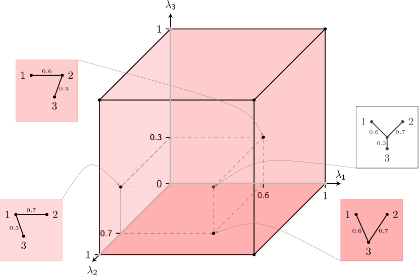
Abbreviating $\lambda_{e_{i}}=\lambda_{i}$ for $i=1,2,3$ we have $\mathcal{G}_{E}\cong(0,1)^{3}$, cf. Equation 2.8, and the map $\bar{\phi}_{E}\colon[0,1]^{3}\to\mathcal{S}$ from Equation 3.5 has the form

$$\bar{\phi}_{E}(\lambda)=\begin{pmatrix}1&\rho_{12}&\rho_{13}\\ \rho_{12}&1&\rho_{23}\\ \rho_{13}&\rho_{23}&1\end{pmatrix}=\begin{pmatrix}1&(1-\lambda_{1})(1-\lambda_{2})&(1-\lambda_{1})(1-\lambda_{3})\\ (1-\lambda_{1})(1-\lambda_{2})&1&(1-\lambda_{2})(1-\lambda_{3})\\ (1-\lambda_{1})(1-\lambda_{3})&(1-\lambda_{2})(1-\lambda_{3})&1\end{pmatrix}\,.$$

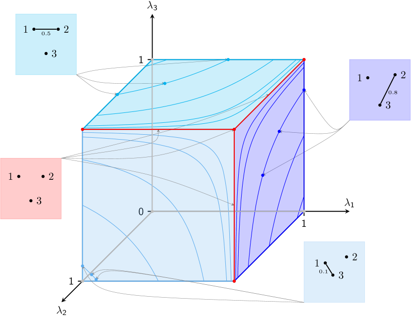
One can easily see from Lemma 3.1.10 that $\bar{\phi}_{E}(\lambda)\in\mathcal{P}$ if and only if at most one coordinate of $\lambda$ is zero, otherwise there would exist $u,v\in L$ with $u\neq v$ such that $\rho_{uv}=1$. This means that the origin and the intersections of the coordinate axes with the cube $[0,1]^{3}$ are not mapped into $\phi(\mathcal{W})$ and thus not part of the boundary of $\mathcal{G}_{E}$. The cube and the corresponding wälder $F^{\prime}\in\mathcal{W}$ of the grove’s boundaries (i.e. there exists $\lambda\in\partial([0,1]^{E})$ with $\bar{\phi}_{E}(\lambda)=\phi(F^{\prime})$) are depicted in Figure 9.

Note that for the boundaries where at least one $\lambda$ coordinate is one, infinitely many coordinates give the same wald: let $F^{\prime}=(\{2|3\},\lambda^{\prime})$ with $\lambda^{\prime}_{2|3}=0.8$, then all coordinates $\lambda^{*}=(1,\lambda_{2}^{*},\lambda_{3}^{*})\in\partial([0,1]^{E})$ that satisfy $1-(1-\lambda_{2}^{*})(1-\lambda_{3}^{*})=0.8$ give $\bar{\phi}_{E}(\lambda^{*})=\phi(F^{\prime})$. This is also illustrated in Figure 9 (right panel), where several arrows point to the coordinates on curves that correspond the same wald. This means that a two-dimensional boundary of the cube collapses into a one-dimensional grove.

If at least two coordinates of $\lambda^{*}$ are equal to 1, then the corresponding phylogenetic forest will be the forest consisting of three isolated vertices, and in this case, four points as well as the three segments where two coordinates are $1$ and one is strictly between zero and one on the boundary of the cube collapse to only one point in $\mathcal{W}$, marked red in Figure 9 (right panel).

Figure 9. Depicting the grove $\mathcal{G}_{E}\cong(0,1)^{3}$ of a fully resolved tree with $N=3$ leaves, and its boundary $\partial\mathcal{G}_{E}$, as discussed in Example 3.2.9. Left: $\mathcal{G}_{E}$ and its two-dimensional “boundary at zero” (coordinate axes are excluded). Right: the “boundary at one” comprising the one-dimensional component (points on same blue curves represent a single wald) and zero-dimensional component (points on the red spider) represent $F_{\infty}$.

Corollary 3.2.10.

Let $F,F^{\prime}\in\mathcal{W}$ with topologies $E,E^{\prime}$, respectively, and let $(F_{n})_{n\in\mathbb{N}}\subset\mathcal{G}_{E}\subset\mathcal{W}$ be a sequence. If $F_{n}\to F^{\prime}$, then $E^{\prime}\leq E$.

Proof.

Let $\lambda^{(n)}\in(0,1)^{E}\cong\mathcal{G}_{E}$ such that $\phi_{E}(\lambda^{(n)})=\phi(F_{n})$ for all $n\in\mathbb{N}$. With the same argument as in the proof of Theorem 3.1.12, there exists at least one subsequence $(\lambda^{(n_{k})})_{k\in\mathbb{N}}$ such that $\lambda^{(n_{k})}\to\lambda^{*}\in[0,1]^{E}$ with $\bar{\phi}_{E}(\lambda^{*})=\phi(F^{\prime})\in\mathcal{P}$, so either $F^{\prime}\in\mathcal{G}_{E}$, then $E^{\prime}=E$, or $F^{\prime}\in\partial\mathcal{G}_{E}$ (by definition of $\partial\mathcal{G}_{E}$ from Equation 3.9), then by Theorem 3.2.7 it follows that $E^{\prime}<E$, so in general $E^{\prime}\leq E$. ∎

3.3. Whitney Stratification of wald space

Recall from Section 1.3 the differentiable manifold of strictly positive definite matrices $\mathcal{P}$, and that the tangent space $T_{P}\mathcal{P}$ at $P\in\mathcal{P}$ is isomorphic to the vector space of symmetric matrices $\mathcal{S}$. In order to study convergence of linear subspaces of $\mathcal{S}$, we recall the Grassmannian manifold of $k$-dimensional linear subspaces in $\mathbb{R}^{m}$, $0\leq k\leq m$, see e.g. (Lee, 2018, Chapter 7).

Every $k$-dimensional linear subspace $\mathcal{V}$ of $\mathbb{R}^{m}$ is the span of the columns $v_{1},\ldots,v_{k}$ of a matrix $(v_{1},\ldots,v_{k})=V\in S(m,k)$, the column space,

$$\mathcal{V}=\mathrm{span}\{v_{1},\ldots,v_{k}\}=\mathrm{col}(V)$$

where

$$S(m,k)=\{V\in\mathbb{R}^{m\times k}:\mathrm{rank}(V)=k\}$$

is the Stiefel manifold of maximal rank $(m\times k)$-matrices equipped with the smooth manifold structure inherited from embedding in the Euclidean $\mathbb{R}^{m\times k}$. Since $\mathrm{col}(V)=\mathrm{col}(VG)$ for every $G\in S(k,k)$ and $V\in S(k,m)$, the space

$$\big{\{}\mathcal{V}\subset\mathbb{R}^{m}\colon\mathcal{V}\text{ linear subspace},\dim(\mathcal{V})=k\big{\}}$$

can be identified with the Grassmannian

$$G(m,k)\coloneqq S(m,k)/S(k,k)\,.$$

As every orbit $\{VG:G\in S(k,k)\}$ of $V\in S(m,k)$ is closed in $S(m,k)$ and since for every $V\in S(m,k)$ its isotropy group $\{G\in S(k,k):VG=V\}$ contains the unit matrix only, the quotient carries a canonical smooth manifold structure.

Definition 3.3.1.

With the above notation, a sequence of $k$-dimensional linear subspaces $\mathcal{V}_{n}$ , $n\in\mathbb{N}$, of $\mathbb{R}^{m}$, $1\leq k<m$, converges in the Grassmannian $G(m,k)$ to a $k$-dimensional linear subspace $\mathcal{V}$ if there are $V_{n},V\in S(m,k)$ and $G_{n}\in S(k,k)$ such that

$$\mathrm{col}(V_{n})=\mathcal{V}_{n}\mbox{ for all }n\in\mathbb{N},~{}\mathrm{col}(V)=\mathcal{V}\mbox{ and }\|V_{n}G_{n}-V\|\to 0\mbox{ as }n\to\infty\,.$$

Remark 3.3.2.

1) Note that none of the cluster points of $G_{n}$ or $G_{n}/\|G_{n}\|$ can be singular, hence they are all in $S(k,k)$

2) There may be, however, a sequence $V_{n}\in S(m,k)$ and $V\in S(m,k)$, $W\in\mathbb{R}^{m\times k}\setminus S(m,k)$ with

$$\mathrm{col}(V_{n})=\mathcal{V}_{n}\to\mathcal{V}=\mathrm{col}(V)$$

in the Grassmanian $G(m,k)$ but

$$\|V_{n}-W\|\to 0$$

in $\mathbb{R}^{m\times k}$. Nevertheless we have the following relationship.

Lemma 3.3.3.

Let $V_{n}\in S(m,k)$ and assume that the two limits below exist. Then

$$\mathrm{col}\left(\lim_{n\to\infty}V_{n}\right) \subseteq \lim_{n\to\infty}\mathrm{col}(V_{n})\,.$$

Proof.

Let $v\in\mathbb{R}^{m}$ with $v\perp\lim_{n\to\infty}\mathrm{col}(V_{n})$. Then the assertion follows, once we show $v\perp W$ with $W=\lim_{n\to\infty}V_{n}$.

By hypothesis, for every $\epsilon>0$ there are $N\in\mathbb{N}$ and $G_{n}\in S(k,k)$ such that

$$|v^{T}V_{n}G_{n}|<\epsilon~{}\forall n>N\,.$$

Let us first assume that there is a subsequence $n_{k}$ with $\|G_{n_{k}}\|>1$. Then

$$|v^{T}V_{n_{k}}R_{n_{k}}|<\frac{\epsilon}{\|G_{n_{k}}\|}<\epsilon~{}\forall n_{k}>N\,,$$

where $R_{n_{k}}=\frac{G_{n_{k}}}{\|G_{n_{k}}\|}\in S(k,k)$ is of unit norm, hence it has a cluster point $R$ satisfying $|v^{T}WR|\leq\epsilon$. As $\epsilon>0$ was arbitrary, we have $v^{T}WR=0$. Since $R\in S(k,k)$ by Remark 3.3.2 we have thus $v^{T}W=0$ as asserted.

If there is no such subsequence, w.l.o.g. we may assume $\|G_{n}\|\leq 1$ for all $n\geq N$. Again, $G_{n}$ has a cluster point $R$ and thus $|v^{T}WR|\leq\epsilon$ which implies, as above, $v^{T}WR=0$. Since $R\in S(k,k)$ by Remark 3.3.2 we have $v^{T}W=0$ as asserted.

∎

In the following, recall the definition of a Whitney stratified space of type (A) and (B), respectively, taken from the wording of Huckemann and Eltzner (2020, Section 10.6).

Definition 3.3.4.

A stratified space $\mathcal{S}$ of dimension $m$ embedded in a Euclidean space (possibly of higher dimension $M\geq m$) is a direct sum

$$\mathcal{S}=\bigsqcup_{i=1}^{k}S_{i}$$

such that $0\leq d_{1}<\ldots<d_{k}=m$, each $S_{i}$ is a $d_{i}$-dimensional manifold and $S_{i}\cap S_{j}=\emptyset$ for $i\neq j$ and if $S_{i}\cap\overline{S_{j}}\neq\emptyset$ then $S_{i}\subset\overline{S_{j}}$.

A stratified space $\mathcal{S}$ is Whitney stratified of type (A),

• if for a sequence $q_{1},q_{2},\dots\in S_{j}$ that converges to some point $p\in S_{i}$, such that the sequence of tangent spaces $T_{q_{n}}S_{j}$ converges in the Grassmannian $G(M,d_{j})$ to a $d_{j}$-dimensional linear space $T$ as $n\to\infty$, then $T_{p}S_{i}\subseteq T$, where all the linear spaces are seen as subspaces of $\mathbb{R}^{M}$.

Moreover, a stratified space $\mathcal{S}$ is a Whitney stratified space of type (B),

• if for sequences $p_{1},p_{2},\dots\in S_{i}$ and $q_{1},q_{2},\dots\in S_{j}$ which converge to the same point $p\in S_{i}$ such that the sequence of secant lines $c_{n}$ between $p_{n}$ and $q_{n}$ converges to a line $c$ as $n\to\infty$ (in the Grassmannian $G(M,1)$), and such that the sequence of tangent planes $T_{q_{n}}S_{j}$ converges to a $d_{j}$-dimensional plane $T$ as $n\to\infty$ (in the Grassmannian $G(M,d_{j})$), then $c\subset T$.

Theorem 3.3.5.

Wald space with the smooth structure on every grove $\mathcal{G}_{E}$ conveyed by $\phi_{E}$ from (3.4), is a Whitney stratified space of type (A).

Proof.

First, we show that $\mathcal{W}$ is a stratified space. In conjunction with Remark 2.2.4, the manifolds $S_{i}$ of dimension $d_{i}=i$ are the unions over disjoint groves of $\mathcal{W}$ of equal dimenison $i=0,\dots,2N-3=m$, counting the number of edges, each diffeomorphic to an $i$-dimensional open unit cube,

$$S_{i}=\bigsqcup_{|E|=i}\mathcal{G}_{E}\,.$$

If $S_{i}\cap\overline{S_{j}}\neq\emptyset$ for some $0\leq i\neq j\leq m$ then there are wald topologies $E,E^{\prime}$ with $j=|E|$, $i=|E^{\prime}|$ and $\mathcal{G}_{E^{\prime}}\cap\in\overline{\mathcal{G}_{E}}\neq\emptyset$, implying $\mathcal{G}_{E^{\prime}}\subset\overline{\mathcal{G}_{E}}$ by Theorem 3.2.7. In particular, then $i<j$. Further, if $\widetilde{E}^{\prime}$ with $i=|E^{\prime}|$ is any other wald topology, induction on Lemma 3.2.6 (xiii) shows that it can be extended to a wald topology $\widetilde{E}$ with $j=|E|$ such that $\widetilde{E}^{\prime}<\widetilde{E}$ and hence $\mathcal{G}_{\widetilde{E}^{\prime}}\subset\overline{\mathcal{G}_{\widetilde{E}^{\prime}}}$ by Theorem 3.2.7. Thus, we have shown that $S_{i}\subset\overline{S_{j}}$, as required.

In order to show Whitney condition (A), it suffices to assume $i\neq j$. Let $F_{1},F_{2},\dots\in S_{j}$ be a sequence of wälder that converges to some wald $F^{\prime}=(E^{\prime},\lambda^{\prime})\in S_{i}$, so $i<j$. Since $S_{j}$ is a disjoint union of finitely many groves, w.l.o.g. we may assume that $F_{1},F_{2},\dots\in\mathcal{G}_{E}$ for some wald topology $E>E^{\prime}$ with $|E|=j$. Hence, under the hypothesis that $T_{F_{n}}\mathcal{G}_{E}\cong T_{\Phi(F_{n})}\Phi_{E}(\mathcal{G}_{E})\subset\mathcal{S}$ converges in the Grassmannian $G(\dim(\mathcal{S}),j)$, to a $j$-dimensional linear space $T\subset\mathcal{S}$ as $n\to\infty$, we need to show that

(3.15) $$T_{F^{\prime}}\mathcal{G}_{E^{\prime}}\cong T_{\Phi(F^{\prime})}\Phi_{E^{\prime}}(\mathcal{G}_{E^{\prime}})\subseteq T\,.$$

With the analytic continuation $\bar{\phi}_{E}$ of $\phi_{E}$, see Remark 3.1.8, a cluster point $\lambda^{*}\in[0,1]^{E}$ of $\lambda^{(n)}=\phi_{E}^{-1}(F_{n})\in(0,1)^{E}$, $F^{\prime}=\phi^{-1}\circ\bar{\phi}_{E}(\lambda^{*})$, see Theorem 3.1.12, and the unit standard basis $\partial/\partial\lambda_{e}$, $e\in E$ of $\mathcal{G}_{E}\cong(0,1)^{E}$ we have thus

$$T_{\Phi(F_{n})}\Phi_{E}(\mathcal{G}_{E})=\operatorname{span}\bigg{\{}\frac{\partial\bar{\phi}_{E}}{\partial\lambda_{e}}\big{(}\lambda^{(n)}\big{)}\colon e\in E\bigg{\}}\,$$

and, due to Lemma 3.3.3,

$$\operatorname{span}\bigg{\{}\frac{\partial\bar{\phi}_{E}}{\partial\lambda_{e}}\big{(}\lambda^{*}\big{)}\colon e\in E\bigg{\}} =\operatorname{span}\bigg{\{}\lim_{n\to\infty}\frac{\partial\bar{\phi}_{E}}{\partial\lambda_{e}}\big{(}\lambda^{(n)}\big{)}\colon e\in E\bigg{\}}$$

$$\subseteq\lim_{n\to\infty}\operatorname{span}\bigg{\{}\frac{\partial\bar{\phi}_{E}}{\partial\lambda_{e}}\big{(}\lambda^{(n)}\big{)}\colon e\in E\bigg{\}}=T.$$

Since likewise

$$T_{\phi(F^{\prime})}\phi(\mathcal{G}_{E^{\prime}})=\operatorname{span}\bigg{\{}\frac{\partial\phi_{E^{\prime}}}{\partial\lambda^{\prime}_{e^{\prime}}}(\lambda^{\prime})\colon e^{\prime}\in E^{\prime}\bigg{\}}$$

showing assertion (3.15) is equivalent to showing

$$\operatorname{span}\bigg{\{}\frac{\partial\phi_{E^{\prime}}}{\partial\lambda^{\prime}_{e^{\prime}}}(\lambda^{\prime})\colon e^{\prime}\in E^{\prime}\bigg{\}}\subseteq\operatorname{span}\bigg{\{}\frac{\partial\bar{\phi}_{E}}{\partial\lambda_{e}}\big{(}\lambda^{*}\big{)}\colon e\in E\bigg{\}}\,.$$

To see this, it suffices to show that for each $e^{\prime}\in E^{\prime}$, there exists a constant $c>0$ and an edge $e\in E$ such that

(3.16) $$\frac{\partial\phi_{E^{\prime}}}{\partial\lambda^{\prime}_{e^{\prime}}}(\lambda^{\prime})=c\,\frac{\partial\bar{\phi}_{E}}{\partial\lambda_{e}}(\lambda^{*}).$$

In the following we show (3.16).

Recalling for $u,v\in L$

$$\Big{(}\bar{\phi}_{E}(\lambda^{*})\Big{)}_{uv}=\prod_{e\in E(u,v)}\big{(}1-\lambda^{*}_{e}\big{)}\,,\quad\Big{(}\phi_{E^{\prime}}(\lambda^{\prime})\Big{)}_{uv}=\prod_{e^{\prime}\in E^{\prime}(u,v)}\big{(}1-\lambda^{\prime}_{e^{\prime}}\big{)}$$

from Definition 3.1.7, obtain their derivatives

(3.17) $$\bigg{(}\frac{\partial\bar{\phi}_{E}}{\partial\lambda_{e}}(\lambda^{*})\bigg{)}_{uv} =-\mathbf{1}_{e\in E(u,v)}\prod_{\begin{subarray}{c}\tilde{e}\in E(u,v)\\ \tilde{e}\neq e\end{subarray}}\big{(}1-\lambda^{*}_{\tilde{e}}\big{)},$$

(3.18) $$\bigg{(}\frac{\partial\phi_{E^{\prime}}}{\partial\lambda^{\prime}_{e^{\prime}}}(\lambda^{\prime})\bigg{)}_{uv} =-\mathbf{1}_{e^{\prime}\in E^{\prime}(u,v)}\prod_{\begin{subarray}{c}\tilde{e}^{\prime}\in E^{\prime}(u,v)\\ \tilde{e}^{\prime}\neq e^{\prime}\end{subarray}}\big{(}1-\lambda^{\prime}_{\tilde{e}^{\prime}}\big{)}.$$

Recall from Corollary 3.2.8 the two relationships between $F^{\prime}$ and $\bar{\phi}_{E}(\lambda^{*})$:

$$E^{\prime}_{\alpha^{\prime}}=\big{\{}e^{\prime}\colon e^{\prime}=e|_{L^{\prime}_{\alpha^{\prime}}}\text{ is a valid split of }L^{\prime}_{\alpha^{\prime}},e\in E\text{ and }\lambda^{*}_{e}\neq 0\big{\}}$$

as well as for each $e^{\prime}\in E^{\prime}$,

(3.19) $$\lambda^{\prime}_{e^{\prime}}=1-\prod_{e\in R_{e^{\prime}}}(1-\lambda^{*}_{e})\neq 0.$$

Consequently, for any $e^{\prime}\in E^{\prime}_{\alpha^{\prime}}$ there exists $e\in R_{e^{\prime}}$ with $\lambda^{*}_{e}\neq 0$.

Now, let $u,v\in L$ be arbitrary and for every $e^{\prime}\in E^{\prime}$, we consider $e$ as above.

1. Case $e\notin E(u,v)$. Then $(\bar{\phi}_{E}(\lambda^{*}))_{uv}$ is constant as $\lambda_{e}$ varies and since $R_{e^{\prime}}\ni e\not\in E(u,v)$, i.e. $R_{e^{\prime}}\not\subseteq E(u,v)$, we have $e^{\prime}\not\in E^{\prime}(u,v)$ by Lemma 3.2.6 (viii) so that likewise $(\phi_{E^{\prime}}(\lambda^{\prime}))_{uv}$ is constant as $\lambda^{\prime}_{e^{\prime}}$ varies, yielding

   $$\bigg{(}\frac{\partial\phi_{E^{\prime}}}{\partial\lambda^{\prime}_{e^{\prime}}}(\lambda^{\prime})\bigg{)}_{uv}=0=\bigg{(}\frac{\partial\bar{\phi}_{E}}{\partial\lambda_{e}}(\lambda^{*})\bigg{)}_{uv}.$$

   Thus for $c$ in (3.16) any positive constant can be chosen.

2. Case $e=A|B\in E(u,v)$. W.l.o.g. assume that $u\in A$ and $v\in B$. Then there are two subcases:

   1. $e^{\prime}\notin E^{\prime}(u,v)$. On the one hand, as above this implies $\big{(}\frac{\partial\phi_{E^{\prime}}}{\partial\lambda^{\prime}_{e^{\prime}}}(\lambda^{\prime})\big{)}_{uv}=0$, on the other hand, as $e^{\prime}=A\cap L^{\prime}_{\alpha^{\prime}}|B\cap L^{\prime}_{\alpha^{\prime}}\notin E^{\prime}(u,v)$, either $u\notin L^{\prime}_{\alpha^{\prime}}$ or $v\notin L^{\prime}_{\alpha^{\prime}}$, implying

      $$0=\big{(}\phi_{E^{\prime}}(\lambda^{\prime})\big{)}_{uv}=\big{(}\bar{\phi}_{E}(\lambda^{*})\big{)}_{uv}=\prod_{\tilde{e}\in E(u,v)}\big{(}1-\lambda^{*}_{\tilde{e}}\big{)}\,.$$

      Thus $\lambda^{*}_{\tilde{e}}=1$ for some $\tilde{e}\in E(u,v)$ with $\tilde{e}\neq e$ (recall that $\lambda^{*}_{e}<1$ for otherwise $\lambda^{\prime}_{e^{\prime}}=1$ by (3.19)), which implies in conjunction with (3.17) that

      $$\bigg{(}\frac{\partial\bar{\phi}_{E}}{\partial\lambda_{e}}(\lambda^{*})\bigg{)}_{uv}=0=\bigg{(}\frac{\partial\phi_{E^{\prime}}}{\partial\lambda^{\prime}_{e^{\prime}}}(\lambda^{\prime})\bigg{)}_{uv}.$$

      Again, for $c$ in (3.16)) any positive constant can be chosen.

   2. $e^{\prime}\in E^{\prime}(u,v)$. Then Lemma 3.2.6 (viii) yields $R_{e^{\prime}}\subseteq E(u,v)$ and we have, invoking (3.18) as well as (3.19), that

      (3.20) $$\bigg{(}\frac{\partial\phi_{E^{\prime}}}{\partial\lambda^{\prime}_{e^{\prime}}}(\lambda^{\prime})\bigg{)}_{uv}~{}=~{}-\prod_{\begin{subarray}{c}\tilde{e}^{\prime}\in E^{\prime}(u,v)\\ \tilde{e}^{\prime}\neq e^{\prime}\end{subarray}}\big{(}1-\lambda^{\prime}_{\tilde{e}^{\prime}}\big{)} = -\prod_{\begin{subarray}{c}\tilde{e}^{\prime}\in E^{\prime}(u,v)\\ \tilde{e}^{\prime}\neq e^{\prime}\end{subarray}}\prod_{\tilde{e}\in R_{\tilde{e}^{\prime}}}\big{(}1-\lambda^{*}_{\tilde{e}}\big{)}\$$

      $$= -\prod_{\begin{subarray}{c}\tilde{e}\in E(u,v)\\ \tilde{e}\notin R_{e^{\prime}}\end{subarray}}\big{(}1-\lambda^{*}_{\tilde{e}}\big{)}\,,$$

      where the last equality follows from observing that $\tilde{e}\notin R_{e^{\prime}}\Leftrightarrow\exists\tilde{e}^{\prime}\in E^{\prime},\tilde{e}^{\prime}\neq e^{\prime}\mbox{ such that }\tilde{e}\in R_{\tilde{e}^{\prime}}$, due to Lemma 3.2.6 (vi). Furthermore, again by (3.17), recalling from above that $R_{e^{\prime}}\subseteq E(u,v)$ and (3.20),

      $$\bigg{(}\frac{\partial\bar{\phi}_{E}}{\partial\lambda_{e}}(\lambda^{*})\bigg{)}_{uv} =-\prod_{\begin{subarray}{c}\tilde{e}\in E(u,v)\\ \tilde{e}\neq e\end{subarray}}\big{(}1-\lambda^{*}_{\tilde{e}}\big{)}$$

      $$=-\bigg{(}\prod_{\begin{subarray}{c}\tilde{e}\in R_{e^{\prime}}\\ \tilde{e}\neq e\end{subarray}}\big{(}1-\lambda^{*}_{\tilde{e}}\big{)}\bigg{)}\bigg{(}\prod_{\begin{subarray}{c}\tilde{e}\in E(u,v)\\ \tilde{e}\notin R_{e^{\prime}}\end{subarray}}\big{(}1-\lambda^{*}_{\tilde{e}}\big{)}\bigg{)}$$

      $$=\bigg{(}\prod_{\begin{subarray}{c}\tilde{e}\in R_{e^{\prime}}\\ \tilde{e}\neq e\end{subarray}}\big{(}1-\lambda^{*}_{\tilde{e}}\big{)}\bigg{)}\bigg{(}\frac{\partial\phi_{E^{\prime}}}{\partial\lambda^{\prime}_{e^{\prime}}}(\lambda^{\prime})\bigg{)}_{uv}\,.$$

      Thus

      $$c=\prod_{\begin{subarray}{c}\tilde{e}\in R_{e^{\prime}}\\ \tilde{e}\neq e\end{subarray}}\big{(}1-\lambda^{*}_{\tilde{e}}\big{)}$$

      satisfies (3.16) as it does not depend on $u$ and $v$ and is non-zero by Equation 3.19.

Having thus shown (3.16), as detailed above we have established (3.15) thus verifying Whitney condition (A). ∎

Whitney condition (B) is a conjecture.

4. Information Geometry for Wald Space

In Garba et al. (2021) we equipped the space of phylogenetic forests with a metric induced from the metric of the Fisher-information Riemannian metric $g$ on $\mathcal{P}$ (see Section 1.3), where the latter induces the metric $d_{\mathcal{P}}$ on $\mathcal{P}$. In this section we show, first that this induced metric is compatible with the stratification structure of $\mathcal{W}$, and second that this turns $\mathcal{W}$ into a geodesic Riemann stratified space.

4.1. Induced Intrinsic Metric

In Garba et al. (2021) we introduced a metric on $\mathcal{W}$ induced from the geodesic distance metric $d_{\mathcal{P}}$ of $\mathcal{P}$ introduced in Section 1.3. Recalling also the definition of path length $L_{\mathcal{P}}$ from Section 1.3, for two wälder $F,F^{\prime}\in\mathcal{W}$, set

$$d_{\mathcal{W}}(F,F^{\prime}):=\inf_{\begin{subarray}{c}\gamma\colon[0,1]\to\mathcal{W}\\ \phi\circ\gamma\text{ continuous in }\mathcal{P},\\ \gamma(0)=F,\gamma(1)=F^{\prime}\end{subarray}}L_{\mathcal{P}}(\phi\circ\gamma)\,.$$

This metric defines the induced intrinsic metric topology on $\mathcal{W}$. While in general this topology may be finer than the one conveyed by making an embedding a homeomorphism, as the following example teaches, this is not the case for wald space.

Example 4.1.1.

Consider

$$\mathcal{M}:=(\{1\}\times[0,1])\quad\cup\bigcup_{y\in\{1/n:n\in\mathbb{N}\}\cup\{0\}}[-1,1)\times\{y\}\,,$$

an infinite union of half open intervals in $\mathbb{R}^{2}$ connected vertically on the right. In the trace topology where the canonical embedding $\iota:\mathcal{M}\hookrightarrow\mathbb{R}^{2}$ is a homeomorphism, the sequence $q_{n}=(0,1/n)$ converges to $q=(0,0)$. For the induced intrinsic metric

$$d_{\mathcal{M}}(x,y)=\inf_{\begin{subarray}{c}\gamma\colon[0,1]\to\mathcal{M}\\ \gamma\text{ continuous in }\mathbb{R}^{2},\\ \gamma(0)=x,\gamma(1)=y\end{subarray}}L_{\mathbb{R}^{2}}(\gamma)\,,$$

with the Euclidean length $L_{\mathbb{R}^{2}}$, we have, however, $d_{W}(q_{n},q)\geq 2$ for all $n\in\mathbb{N}$.

Theorem 4.1.2.

The topology of $\mathcal{W}$ obtained from making $\phi$ a homeomorphism agrees with the topology induced from the induced intrinsic metric $d_{\mathcal{W}}$. In particular $d_{\mathcal{W}}$ turns $\mathcal{W}$ into a metric space.

Proof.

By definition we have that $d_{\mathcal{W}}\geq d_{\mathcal{P}}$, which implies that sequences that converge with respect to $d_{\mathcal{W}}$ also converge with respect to $d_{\mathcal{P}}$.

For the converse, assume that $\mathcal{W}\ni F_{n}\to F^{\prime}\in\mathcal{W}$ w.r.t. $d_{\mathcal{P}}$, as $n\to\infty$. Since there are only finitely many groves in $\mathcal{W}$ it suffices to show that $d_{\mathcal{W}}(F_{n},F)\to 0$ for $F_{n}\in\mathcal{G}_{E}$ and $F\in\overline{\mathcal{G}_{E}}$ with a common grove $\mathcal{G}_{E}$. Hence, we assume that $\bar{\phi}^{-1}_{E}\circ\phi(F_{n})=\lambda_{n}\in(0,1)^{E}$ and $\bar{\phi}^{-1}_{E}\circ\phi(F^{\prime})=\lambda^{\prime}\in[0,1]^{E}$ with $\lambda_{n}\to\lambda^{\prime}$, due to Theorem 3.1.12. Then, with $\delta(t)=t\lambda^{\prime}+(1-t)\lambda_{n}$,

$$\gamma:[0,1]\to\mathcal{P},t\mapsto\phi^{-1}\circ\bar{\phi}_{E}\circ\delta(t))=:\gamma(t)$$

is a path in $\mathcal{W}$ connecting $\gamma(0)=F$ with $\gamma(1)=F_{n}$. For $k\in\mathbb{N}$ and $j=1,\ldots,k$ we note that

$$\bar{\phi}_{E}\circ\delta_{n}\left(\frac{j}{k}\right) = \bar{\phi}_{E}\circ\delta_{n}\left(\frac{j-1}{k}\right)+(D\bar{\phi}_{E})\circ\delta_{n}\left(\frac{j-1}{k}\right)\cdot\frac{\lambda^{\prime}-\lambda_{n}}{k}+o\left(\frac{\|\lambda^{\prime}-\lambda_{n}\|}{k}\right)$$

where both terms

$$\bar{\phi}_{E}\circ\delta_{n}\left(\frac{j-1}{k}\right),(D\bar{\phi}_{E})\circ\delta_{n}\left(\frac{j-1}{k}\right)$$

are bounded, also uniformly $n\in\mathbb{N}$, due to Remark 3.1.8. In consequence, in conjunction with Section 1.3,

$$d_{\mathcal{W}}(F_{n},F)$$

$$\leq \lim_{k\to\infty}\sum_{j=1}^{k}d_{\mathcal{P}}\left(\bar{\phi}_{E}\circ\delta\left(\frac{j-1}{k}\right),\bar{\phi}_{E}\circ\delta\left(\frac{j}{k}\right)\right)$$

$$= \lim_{k\to\infty}\sum_{j=1}^{k}\left\|\log\left(\sqrt{\bar{\phi}_{E}\circ\delta\left(\frac{j-1}{k}\right)}^{-1}\bar{\phi}_{E}\circ\delta_{n}\left(\frac{j}{k}\right)\sqrt{\bar{\phi}_{E}\circ\delta_{n}\left(\frac{j-1}{k}\right)}^{-1}\right)\right\|$$

$$\leq C\|\lambda^{\prime}-\lambda_{n}\|$$

with a constant $C>0$ independent of $n$. Letting $n\to\infty$ thus yields the assertion.

∎

4.2. Geodesic Space and Riemann Stratification

Having established the equivalence between the stratification topology and that of the Fisher information metric, we longer distinguish between them.

Theorem 4.2.1.

The wald space equipped with the information geometry is a geodesic metric space, i.e. every two points in $(\mathcal{W},d_{\mathcal{W}})$ are connected by a minimising geodesic.

Proof.

By (Lang, 1999, p.325), $(\mathcal{P},g)$ is geodesically complete as a Riemannian manifold and thus by the Hopf-Rinow Theorem for Riemannian manifolds (among others, (Lang, 1999, p.224)), it follows that $(\mathcal{P},d_{\mathcal{P}})$ is complete and locally compact. By Corollary 3.1.3, $\phi(\mathcal{W})$ is a closed subset of the complete and locally compact metric space $\mathcal{P}$ and so $(\phi(\mathcal{W}),d_{\mathcal{P}})$ itself is, and so is $(\mathcal{W},d_{\mathcal{P}})$. By (Garba et al., 2021, Theorem 5.1), any two wälder in are connected by a continuous path of finite length in $(\mathcal{W},d_{\mathcal{P}})$, which is complete, and thus applying (Hu and Kirk, 1978, Corollary on p.123) yields that $(\mathcal{W},d_{\mathcal{W}})$ is complete. Applying the Hopf-Rinow Theorem for metric spaces (Bridson and Haefliger, 1999, p.35) to $(\mathcal{W},d_{\mathcal{W}})$, the assertion holds. ∎

Following Huckemann and Eltzner (2020, Section 10.6), extend the notion of a Whitney stratified space in Definition 3.3.4 to the notion of a Riemann stratified space.

Definition 4.2.2.

A Riemann stratified space is a Whitney stratified space $\mathcal{S}$ of type (A) such that each stratum $S_{i}$ is a $d_{i}$-dimensional Riemannian manifold with Riemannian metric $g^{i}$, respectively, if whenever a sequence $q_{1},q_{2},\dots\in S_{j}$ which converges to a point $p\in S_{i}$ (where, assume again that the sequence of tangent planes $T_{q_{n}}S_{j}$ converges to some $d_{j}$-dimensional plane $T$ as $n\to\infty$), then the Riemannian metric $g_{q_{n}}^{j}$ converges to some two form $g_{p}^{*}\colon T\otimes T\to\mathbb{R}$ with $g_{p}^{i}\equiv g_{p}^{*}|_{T_{p}S_{i}\otimes T_{p}S_{i}}$.

Theorem 4.2.3.

The wald space $\mathcal{W}$ equipped with the information geometry is a Riemann stratified space.

Proof.

As we impose the Riemannian metric $g$ from $\mathcal{P}$ onto all of $\phi(\mathcal{W})\subset\mathcal{P}$, the assertion follows immediately. ∎

Example 4.2.4 (Geometry of wald space for $N=2$).

For $N=2$, $L=\{1,2\}$, there is one edge $e=1|2$, and two different topologies, namely

$$E=\{1|2\}\qquad\text{ and }\qquad E^{\prime}=\emptyset.$$

The corresponding groves are then $\phi(\mathcal{G}_{E^{\prime}})=\{I\}$, where $I$ is the $2\times 2$ unit matrix, and $\mathcal{G}_{E}\cong(0,1)$ such that $\mathcal{W}=\mathcal{G}_{E}\sqcup\mathcal{G}_{E^{\prime}}\cong(0,1]$. Using $\lambda\in(0,1)$ for the only edge $e=1|2$ we have

$$\phi(\mathcal{G}_{E})=\bigg{\{}\phi_{E}(\lambda)=\begin{pmatrix}1&1-\lambda\\ 1-\lambda&1\end{pmatrix}\colon\lambda\in(0,1)\bigg{\}},$$

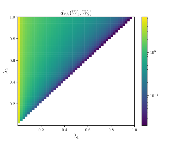
Thus, with the definition of $d_{\mathcal{P}}$ in Section 1.3, the distance between two phylogenetic forests $F_{1}=\bar{\phi}_{E}(\lambda_{1})$, $F_{2}=\bar{\phi}_{E}(\lambda_{2})$ with $\lambda_{1},\lambda_{2}\in(0,1]$ can be calculated as

$$d_{\mathcal{W}}\big{(}F_{1},F_{2}\big{)}=\Bigg{|} \ln\Bigg{(}\frac{1-\lambda_{2}+\frac{1}{\sqrt{2}}p(\lambda_{2})}{1-\lambda_{1}+\frac{1}{\sqrt{2}}p(\lambda_{1})}\Bigg{)}$$

$$+\frac{1}{2\sqrt{2}}\ln\Bigg{(}\frac{\big{(}p(\lambda_{1})+(1-\lambda_{1})\big{)}^{2}-1}{\big{(}p(\lambda_{1})-(1-\lambda_{1})\big{)}^{2}-1}\,\cdot\,\frac{\big{(}p(\lambda_{2})-(1-\lambda_{2})\big{)}^{2}-1}{\big{(}p(\lambda_{2})+(1-\lambda_{2})\big{)}^{2}-1}\Bigg{)}\Bigg{|},$$

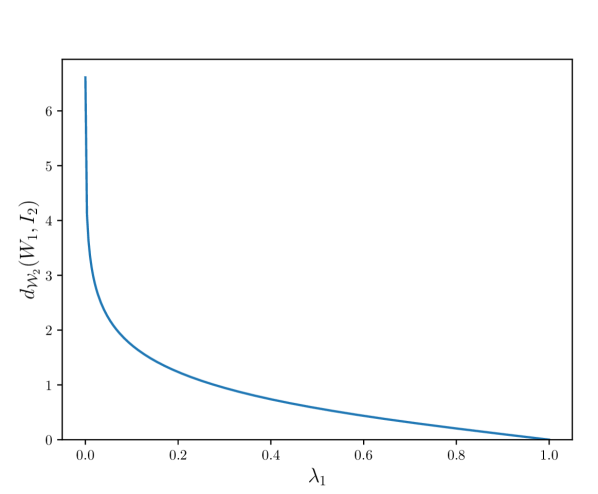
where $p(x)=\sqrt{2}\sqrt{(1-x)^{2}+1}$ for $x\in[0,1]$. Fig. 10 (right) depicts the distance as a function of $\lambda_{1},\lambda_{2}$. We obtain the distance to the disconnected forest $F_{\infty}=\phi^{-1}\bar{\phi}_{E}(1)$:

$$d_{\mathcal{W}}\big{(}F_{1},F_{\infty}\big{)}=\bigg{|}\frac{1}{2\sqrt{2}}\ln\bigg{(}\frac{(p(\lambda_{1})+(1-\lambda_{1}))^{2}-1}{(p(\lambda_{1})-(1-\lambda_{1}))^{2}-1}\bigg{)}-\ln\Big{(}1-\lambda_{1}+\frac{1}{\sqrt{2}}p(\lambda_{1})\Big{)}\bigg{|}.$$

This distance is depicted (as a function in $\lambda_{1}$) in Fig. 10 (left).

Figure 10. Depicting the distance $d_{\mathcal{W}}$ of an arbitrary wald, to the disconnected forest $F_{\infty}$ as a function of $\lambda_{1}$ (left) and between any two other wälder in $\mathcal{W}$, as a function of $(\lambda_{1},\lambda_{2})$ (right) as detailed in Example 4.2.4.

5. Numerical Exploration of Wald Space

In this section we propose a new algorithm to approximate geodesics between two fully resolved trees $F_{1}$ and $F_{2}$, that is a mixture of the successive projection algorithm and the extrinsic path straightening algorithm from Lueg et al. (2021). Using this algorithms allows to explore curvature and so-called stickiness of Fréchet means.

5.1. Approximating Geodesics in Wald Space

From the ambient geometry of $\mathcal{P}$, recalling the notation from Section 1.3, we employ the globally defined Riemannian exponential $\mathrm{Exp}$ and logarithm $\mathrm{Log}$ at $P\in\mathcal{P}$, with $Q\in\mathcal{P}$, $X\in T_{P}\mathcal{P}$, as well as points on the unique (if $P\neq Q$) geodesic $\gamma_{P,Q}$ in $\mathcal{P}$ comprising $P$ and $Q$. Further, $\exp$ and $\log$ denote the matrix exponential and logarithm, respectively:

$$\mathrm{Exp}_{P} \colon T_{P}\mathcal{P}\to\mathcal{P}, X\mapsto\sqrt{P}\exp\big{(}\sqrt{P}^{-1}X\sqrt{P}^{-1}\big{)}\sqrt{P},$$

$$\mathrm{Log}_{P} \colon\mathcal{P}\to T_{P}\mathcal{P}, Q\mapsto\sqrt{P}\log\big{(}\sqrt{P}^{-1}Q\sqrt{P}^{-1}\big{)}\sqrt{P},$$

$$\gamma_{P,Q}^{(\mathcal{P})} \colon[0,1]\to\mathcal{P}, t\mapsto\mathrm{Exp}_{P}\big{(}t\,\mathrm{Log}_{P}(Q)\big{)},$$

Furthermore, for a forest $F\in\mathcal{W}$ with topology $E$, denote the orthogonal projection from the tangent space $T_{P}\mathcal{P}$ at $P=\phi(F)$ onto the tangent space of the sub-manifold $T_{P}\phi_{E}(\mathcal{G}_{E})$, as a subspace of $T_{P}\mathcal{P}$, with

$$\pi_{P}\colon T_{P}\mathcal{P}\to T_{P}\phi_{E}(\mathcal{G}_{E}).$$

This projection is computed using an orthonormal basis of $T_{P}\phi_{E}(\mathcal{G}_{E})$ obtained from applying Gram-Schmidt to the basis

$$\bigg{\{}\frac{\partial\phi_{E}}{\partial\lambda_{e}}(\lambda)\colon e\in E\bigg{\}}.$$

of $T_{P}\phi_{E}(\mathcal{G}_{E})$. Finally, we make use of the projection

$$\pi\colon\mathcal{P}\to\mathcal{W},\qquad P\mapsto\operatorname*{\mbox{\rm argmin}}_{F\in\mathcal{W}}d_{\mathcal{P}}\big{(}P,\phi(F)\big{)},$$

where $\pi$ is well-defined for $P\in\mathcal{P}$ close enough to $\phi(\mathcal{W})$. The following algorithm is similar to the extrinsic path straightening algorithm from Lueg et al. (2021), which has been inspired by Schmidt et al. (2006). It starts with generating a discrete curve using the successive projection algorithm from Lueg et al. (2021) and then iteratively straightening it and adding more points in between the points of the discrete curve. To keep notation simple, we omit $\phi$ and identify a forest $F\in\mathcal{W}$ with its matrix representation $\phi(F)$.

Definition 5.1.1 (Geodesic Approximation Algorithm).

Let $5\leq n_{0}\in\mathbb{N}$ be the odd number of points in the initial path, $I\in\mathbb{N}$ the number of extensions iterations and $J\in\mathbb{N}$ the number of straightening iterations of the path.

Input:

$F,F^{\prime}\in\mathcal{W}$

Initial path:

Set $F_{1}\coloneqq F$, $F_{n_{0}}\coloneqq F^{\prime}$, then, for $i=2,\dots,(n_{0}-3)/2$, compute

$$F_{i} =\pi\bigg{(}\gamma_{F_{i-1},F_{n_{0}-i+2}}\Big{(}\frac{1}{n_{0}-2i+3}\Big{)}\bigg{)},$$

$$F_{n_{0}-i+1} =\pi\bigg{(}\gamma_{F_{n_{0}-i+2},F_{i-1}}\Big{(}\frac{1}{n_{0}-2i+3}\Big{)}\bigg{)},$$

and, with $F_{(n_{0}-1)/2}\coloneqq\pi(\gamma_{F_{(n_{0}-3)/2},F_{(n_{0}+1)/2}}(0.5))$, set the current discrete path to

$$\Gamma\coloneqq\big{(}F_{1},\dots,F_{(n_{0}-3)/2},F_{(n_{0}-1)/2},F_{(n_{0}+1)/2},\dots,F_{n_{0}}\big{)}.$$

Iteratively extend and straighten::

Do $I$ times:

Extend:

With the current discrete path $\Gamma=\big{(}F_{0},\dots,F_{n}\big{)}$, for $i=0,\dots,n-1$ compute $G_{i}\coloneqq\pi\big{(}\gamma_{F_{i},F_{i+1}}(0.5)\big{)}$ and define the new current discrete path

$$\Gamma\coloneqq\big{(}F_{0},G_{0},F_{1},G_{1},\dots,F_{n-1},G_{n-1},F_{n}\big{)}.$$

Do $J$ times:

Straighten:

With the current discrete path $\Gamma=\big{(}F_{0},\dots,F_{n}\big{)}$, for $i=2,\dots,n-1$, compute $X_{i}=\frac{1}{2}\big{(}\mathrm{Log}_{F_{i}}(F_{i-1})+\big{(}\mathrm{Log}_{F_{i}}(F_{i+1})\big{)}$, update $F_{i}\coloneqq\pi\big{(}\mathrm{Exp}_{F_{i}}^{(\mathcal{P})}(X_{i})\big{)}$, and define the new current discrete path

$$\Gamma\coloneqq\big{(}F_{0},F_{1},\dots,F_{n}\big{)}.$$

Return:

The current discrete path $\Gamma$, which is a discrete approximation of the geodesic between $F$ and $F^{\prime}$ with $2^{I}(n_{0}-1)+1$ points.

While Theorem 4.2.1 guarantees the existence of a shortest path between any $F,F^{\prime}\in\mathcal{W}$, it may not be unique, and it is not certain whether the path found by the algorithm is near a shortest path or represents just a local approximation.

To better assess the quality of the approximation $\Gamma=(F_{0},\ldots,F_{n})$ found by the algorithm, Rumpf and Wirth (2015) propose considering its energy,

$$E(\Gamma)=\frac{1}{2}\sum_{i=0}^{n-1}d_{\mathcal{P}}(F_{i},F_{i+1})^{2}\,,$$

yielding a means of comparison for discrete paths with equal number of points.

Example 5.1.2 (Geodesics in wald space for $N=3$).

Revisiting $\mathcal{W}$ from Example 3.2.9 with unique top-dimensional grove $\mathcal{G}_{E}\cong(0,1)^{3}$, we approximate a shortest path between the two phylogenetic forests $F_{1},F_{2}\in\mathcal{W}$ with $\phi(F_{1})=\phi_{E}(\lambda^{(1)})$ and $\phi(F_{2})=\phi_{E}(\lambda^{(2)})$ using the algorithm from Definition 5.1.1, where

$$\lambda^{(1)}=(0.1,0.9,0.07)\qquad\text{ and }\qquad\lambda^{(2)}=(0.3,0.1,0.9).$$

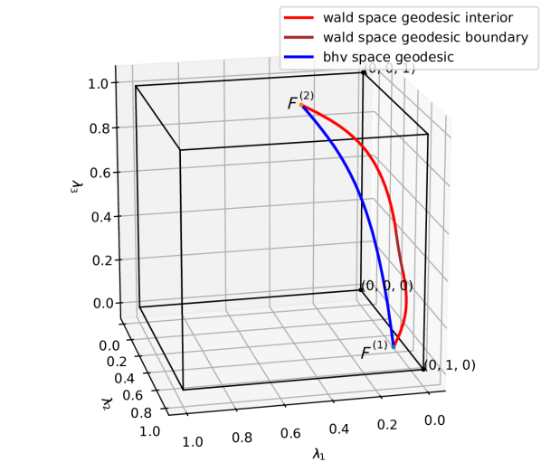
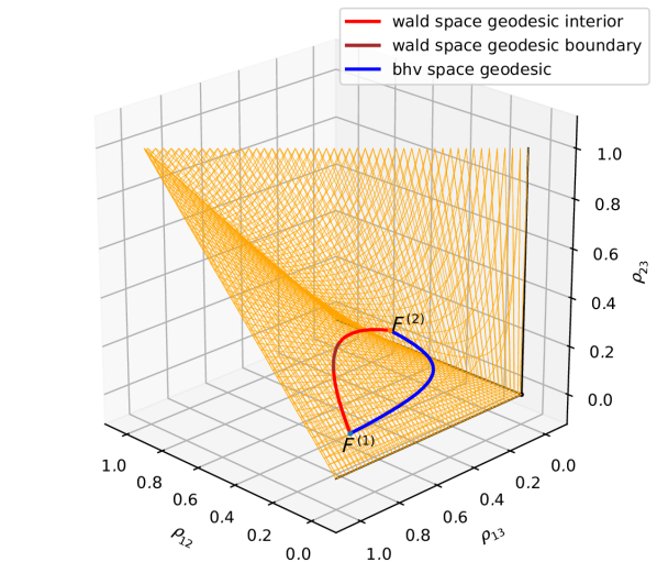
This path is depicted in Figure 11, as well as the BHV space geodesic (which is a straight line with respect to the $\ell$-parametrization from Definition 2.1.2), first in the coordinates $\lambda\in(0,1)^{3}$ and second embedded into $\mathcal{P}$ viewed as $\mathbb{R}^{3}$, cf. Figure 3. In contrast to the BHV geometry, the shortest path in the wald space geometry sojourns on the two-dimensional boundary, where the coordinate $\lambda_{1}$ is zero for some time. The end points $\lambda^{(1)},\lambda^{(2)},$ are trees that show a high level of disagreement over the location of taxon 1, but a similar divergence between taxon 2 and taxon 3. The section of the approximate geodesic with $\lambda_{1}=0$ represents trees on which the overall divergence between taxon 1 and the other two taxa is reduced. In this way, the conflicting information in the end points is resolved by reducing the divergence (and hence increasing the correlation) between taxon 1 and the other two taxa, in comparison to the BHV geodesic which has $\lambda_{1}>0$ along its length.

Figure 11. The wald space geodesic (red) between fully resolved phylogenetic forests $F_{1},F_{2}\in\mathcal{W}$ ($N=3$) sojourns on the boundary (brown). The image of the BHV space geodesic (blue) remains in the grove as discussed in Example 5.1.2. In $\lambda$-representation (left) and embedded in $\mathcal{P}$ viewed as $\mathbb{R}^{3}$ (right, cf. Figure 3).

5.2. Exploring Curvature of Wald Space

Since curvature computations involving higher order tensors are heavy on indices, we keep notation as simple as possible in the following by indexing splits in $E$ by

$$h,i,j,k,m,s,t\in E\,.$$

The concepts of transformation of metric tensors, Christoffel symbols and curvature employed in the following can be found in any standard text book on differential geometry, e.g. Lang (1999); Lee (2018).

Recall that the Riemannian structure of wald space is inherited on each grove $\mathcal{G}_{E}\cong(0,1)^{E}$ from the information geometric Riemann structure of $\mathcal{P}$ pulled back from $\phi_{E}\colon(0,1)^{E}\to\mathcal{P}$. In consequence, the Riemannian metric tensor $g_{\lambda}^{(\mathcal{G}_{E})}$ of $\mathcal{G}_{E}$, evaluated at $\lambda\in(0,1)^{E}$, is given by the Riemannian metric tensor $g_{\lambda}^{\mathcal{P}}$ at $\phi_{E}(\lambda)=P$, where base vectors transform under the derivative of $\phi_{E}$:

$$g^{(\mathcal{G}_{E})}_{\lambda}(x,y)=\sum_{i\in E}\sum_{j\in E}x_{i}y_{j}\;g^{(\mathcal{P})}_{P}\bigg{(}\frac{\partial\phi_{E}}{\partial\lambda_{i}}(\lambda),\,\frac{\partial\phi_{E}}{\partial\lambda_{j}}(\lambda)\bigg{)}$$

for $(x,y)\in T_{\lambda}\mathcal{G}_{E}\times T_{\lambda}\mathcal{G}_{E}\cong\mathbb{R}^{E}\times\mathbb{R}^{E}$ and

$$(\mathrm{d}\phi_{E})_{\lambda}\big{(}T_{\lambda}\mathcal{G}_{E}\big{)}=\operatorname{span}\bigg{\{}\frac{\partial\phi_{E}}{\partial\lambda_{i}}(\lambda)\colon i\in E\bigg{\}}\subseteq T_{P}\mathcal{P}.$$

As usual $(g_{ij})_{i,j\in E}$ denotes the matrix of $g^{(\mathcal{G}_{E})}_{\lambda}$ in standard coordinates and $(g^{ij})_{i,j\in E}$ its inverse. This yields the Christoffel symbols for $i,j,m\in E$,

$$\Gamma_{ij}^{m}=\frac{1}{2}\sum_{k\in E}\bigg{(}\frac{\partial g_{jk}}{\partial\lambda_{i}}+\frac{\partial g_{ki}}{\partial\lambda_{j}}-\frac{\partial g_{ij}}{\partial\lambda_{k}}\bigg{)}g^{km},$$

which give the representation of the curvature tensor

$$R_{ijks}=\sum_{t\in E}\bigg{(}\sum_{h\in E}\Gamma_{ik}^{h}\Gamma_{jh}^{t}-\sum_{h\in E}\Gamma_{jk}^{h}\Gamma_{ih}^{t}+\frac{\partial}{\partial\lambda_{j}}\Gamma_{ik}^{t}-\frac{\partial}{\partial\lambda_{i}}\Gamma_{jk}^{t}\bigg{)}g_{ts}$$

in the coordinates $i,j,k,s\in E$.

Introducing the notation ($P=\phi_{E}(\lambda)$)

$$Q_{i}=P^{-1}\,\frac{\partial\phi_{E}}{\partial\lambda_{i}}(\lambda)\qquad\text{and}\qquad Q_{ij}=P^{-1}\frac{\partial^{2}\phi_{E}}{\partial\lambda_{i}\partial\lambda_{j}}(\lambda)$$

and performing a longer calculation in coordinates $i,j\in E$, gives

$$R_{ijij}=\frac{1}{4} \sum_{a,h\in E}g^{ah}\operatorname*{Tr}\Big{[}\big{(}2Q_{ij}-Q_{j}Q_{i}-Q_{i}Q_{j}\big{)}Q_{a}\Big{]}\operatorname*{Tr}\Big{[}\big{(}2Q_{ij}-Q_{j}Q_{i}-Q_{i}Q_{j}\big{)}Q_{h}\Big{]}$$

$$- \sum_{a,h\in E}g^{ah}\operatorname*{Tr}\Big{[}Q_{i}^{2}Q_{a}\Big{]}\operatorname*{Tr}\Big{[}Q_{j}^{2}Q_{h}\Big{]}$$

$$- \operatorname*{Tr}\Big{[}\big{(}2Q_{ij}-Q_{j}Q_{i}-Q_{i}Q_{j}\big{)}Q_{ij}\Big{]}.$$

Evaluating the sectional curvature tensor at a pair of tangent vectors $x,y\in T_{\lambda}\mathcal{G}_{E}\cong\mathbb{R}^{E}$ at $\lambda$ gives the sectional curvature $K(x,y)$ at $\lambda$ of the local two-dimensional subspace spanned by geodesics with initial directions generated by linear combinations of $x$ and $y$. Abbreviating $|x|_{\lambda}^{(\mathcal{G}_{E})}\coloneqq(g_{\lambda}^{(\mathcal{G}_{E})}(x,x))^{1/2}$ we have

$$K(x,y)=\frac{\sum_{i\in E}\sum_{j\in E}x_{i}y_{i}R_{ijij}}{|x|_{\lambda}^{(\mathcal{G}_{E})}|y|_{\lambda}^{(\mathcal{G}_{E})}-g^{(\mathcal{G}_{E})}_{\lambda}(x,y)}.$$

Example 5.2.1.

Again revisiting $\mathcal{W}$ from Example 3.2.9 with $N=3$, we first consider wälder in the unique top-dimensional grove $\mathcal{G}_{E}\cong(0,1)^{3}$, and then on its boundary.

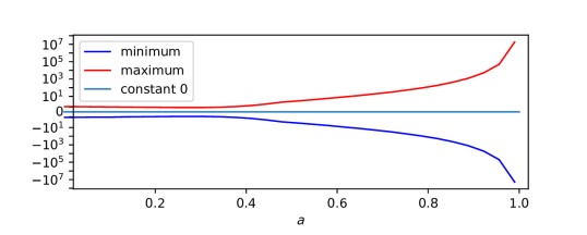
1. We compute minimum and maximum sectional curvatures at the wälder $F$ with $\lambda=(a,a,a)$, for $a\in(0,1)$, as displayed in Figure 12. Traversing along $0<a<1$ we find both positive and negative sectional curvatures and their extremes escape to positive and negative infinity as the vantage point, the isolated forest $F_{\infty}$, is approached, where all dimensions collapse.

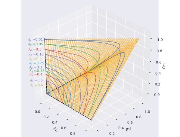
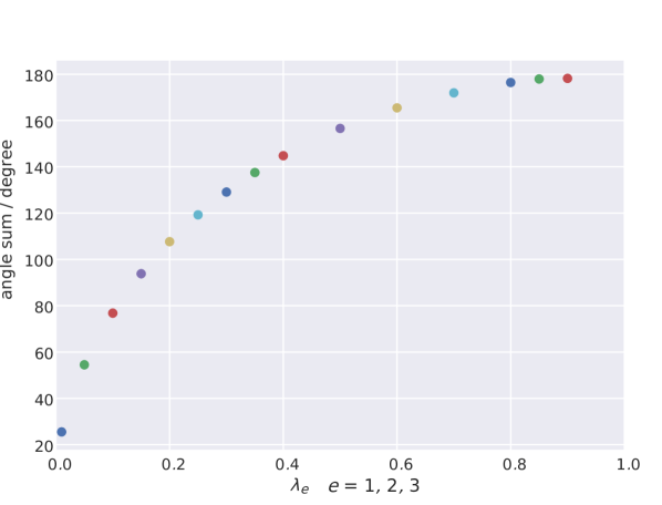
2. In order to assess Alexandrov curvature that measures “fatness/slimless” of geodesic triangles (hence it does not require a Riemannian structure, a geodesic space suffices, see Sturm (2003)) we compute several geodesic triangles and their respective angle sums within $\mathcal{W}$. The corners of the triangles are wälder $F_{1},F_{2},F_{3}\in\mathcal{W}$, where $\{i,j,k\}=\{1,2,3\}$, $E_{i}:=\{j|k\}$ and $\lambda_{j|k}\in(0,1]$. Figure 13 depicts the geodesic triangles (left panel) non isometrically embedded in $\mathbb{R}^{3}$ representing the off-diagonals in $\mathcal{P}$, as well as their respective angle sums (right panel). When the two connected leaves approach one another ($\lambda_{e}\approx 0$) triangles become infinitely thin, but near $F_{\infty}$ ($\lambda_{e}\approx 1$) the triangles become Euclidean.

Figure 12. Minimum and maximum sectional curvatures along $0<a<1$ of wald space ($N=3$) at $F\in\mathcal{W}$ with $\lambda=(a,a,a)$, as described in Example 5.2.1.

Figure 13. Displaying sums of angles in degrees (right) of geodesic triangles spanned by three wälder for $N=3$ with one disconnected leaf and edge weight $0<\lambda_{e}<1$ between the other two leaves as discussed in Example 5.2.1. Embedding $\mathcal{W}$ in $\mathcal{P}$ viewed (non isometrically) as $\mathbb{R}^{3}$, the geodesic triangles are visualized on the left, where the origin corresponds to $\lambda_{e}=1$.

Conjecture 5.2.2.

This example hints towards a general situation:

• Wald space groves feature positive and negative sectional curvatures alike, both of which become unbounded when approaching the vantage point $F_{\infty}$.

• When approaching the infinitely far away boundary of $\mathcal{P}$ from within $\mathcal{W}$, some Alexandrov curvatures tend to negative infinity.

5.3. Exploring Stickiness in Wald Space

Statistical applications in tree space often require the concept of a mean or average tree. Since the expectation of a random variable taking values in a non-Euclidean metric space $(M,d)$ is not well-defined, Fréchet (1948) proposed to resort instead to a minimizer of expected squared distance to a random element $X$ in $M$,

$$p^{*}\in\operatorname*{\mbox{\rm argmin}}_{p\in M}\mathbb{E}[d(p,X)^{2}]\,$$

called a barycenter or Fréchet mean. In a Euclidean geometry, if existent, the Fréchet mean is unique and identical to the expected value of $X$. Given a sample $X_{1},\ldots,X_{n}\stackrel{{\scriptstyle i.i.d.}}{{\sim}}X$, measurable selections from the set

$$\operatorname*{\mbox{\rm argmin}}_{p\in M}\mathcal{F}(p),\quad\mathcal{F}(p):=\frac{1}{n}\sum_{j=1}^{n}d(p,X_{j})^{2}$$

are called empirical Fréchet means and their asymptotic fluctuations allow for nonparametric statistics. Usually, $\mathcal{F}$ is called the empirical Fréchet function.

Recently, it has been discovered by Hotz and Huckemann (2015); Eltzner and Huckemann (2019) that positive curvatures may increase asymptotic fluctuation by orders of magnitude, and by Hotz et al. (2013); Huckemann et al. (2015) that infinite negative Alexandrov curvature may completely cancel asymptotic fluctuation, putting a dead end to this approach of non-Euclidean statistics. In particular, this can be the case for BHV spaces, cf. Barden et al. (2013, 2018); Barden and Le (2018).

Example 5.3.1 (Stickiness in wald space).

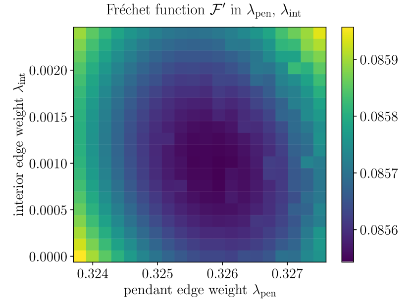
Consider two samples $F_{1},F_{2},F_{3}\in\mathcal{W}$ and $F_{1}^{\prime},F_{2},F_{3}\in\mathcal{W}$ with $N=4$, depicted in Figure 14, where $F_{1}$ and $F_{1}^{\prime}$ only differ by weights of their interior edges. By symmetry, their Fréchet means are of form $F$ having equal but unknown pendent edge weights $0<\lambda_{pen}<1$ and unknown interior edge weights $0\leq\lambda_{int}<1$, as in Figure 14. It turns out that the Fréchet means of both samples agree in BHV with $\lambda_{int}=0$, i.e. the empirical mean sticks to the lower dimensional star tree stratum (featuring only pendant edges).

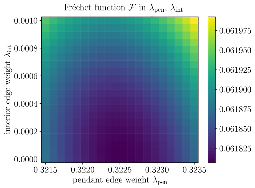
In contrast, the two empirical Fréchet functions in wald space

$$\mathcal{F}(F) = \frac{1}{3}\left(d_{\mathcal{W}}(F,F_{1})^{2}+d_{\mathcal{W}}(F,F_{2})^{2}+d_{\mathcal{W}}(F,F_{3})^{2}\right)$$

$$\mathcal{F}^{\prime}(F) = \frac{1}{3}\left(d_{\mathcal{W}}(F,F^{\prime}_{1})^{2}+d_{\mathcal{W}}(F,F_{2})^{2}+d_{\mathcal{W}}(F,F_{3})^{2}\right)$$

have different minimizers, and, in particular the minimizer for $\mathcal{F}^{\prime}$ does not stick to the star stratum but has $\lambda_{int}>0$. Figure 15 illustrates the values of $\mathcal{F}$ and $\mathcal{F}^{\prime}$ for different values of the parameters $\lambda_{\mathrm{pen}},\lambda_{\mathrm{int}}$ of $F$ near the respective minima.

Figure 14. Two samples of wälder: $F_{1},F_{2},F_{3}$ and $F_{1}^{\prime},F_{2},F_{3}$ where $F_{1}$ and $F_{1}^{\prime}$ only differ by weights of their interior edges. By symmetry, $F$ is a candidate for each Fréchet mean, see Example 5.3.1.

Figure 15. Heat map for the values of the Fréchet functions $\mathcal{F}$ (left) and $\mathcal{F}^{\prime}$ (right) of two samples as functions of $\lambda_{\mathrm{pen}},\lambda_{\mathrm{int}}$ determining candidate minimiziers $F$ as detailed in Example 5.3.1 and illustrated in Figure 14.

Remark 5.3.2.

This preliminary research indicates that effects of stickiness, which are still expected where “too many” lower dimensional strata hit higher dimensional strata, are less severe in wald space than in BHV space, thus making wald space more attractive for asymptotic statistics based on Fréchet means.

6. Discussion

In previous work (Garba et al., 2021), the wald space was introduced as a space for statistical analysis of phylogenetic trees, based on assumptions with a stronger biological motivation than existing spaces. In that work, the focus was primarily on geometry, whereas here we have provided a rigorous characterization of the toplogy of wald space. Specifically, wald space $\mathcal{W}$ is a disjoint union of open cubes with the Euclidean toplogy, and as topological subspaces we have

$$\mathcal{BHV}_{N-1}\subset\mathcal{W}\subset\mathcal{E}_{N}\,$$

with the BHV space $\mathcal{BHV}_{N-1}$ from Billera et al. (2001) and the edge-product space $\mathcal{E}_{N}$ from Moulton and Steel (2004). We have shown that this topology is the same as that induced by the information metric $d_{\mathcal{W}}$ defined in Garba et al. (2021). Furthermore, we have shown $\mathcal{W}$ is contractible, and so does not contain holes or handles of any kind. Examples suggest that $\mathcal{W}$ is a truncated cone in some sense (see Figure 4), but its precise formulation remains an open problem. As established in Theorem 3.3.5, boundaries between strata in wald space satisfy Whitney condition (A); whether Whitney condition (B) holds is an open problem, although we expect it to hold on the boundaries of any grove $(0,1)^{E}\cong\mathcal{G}_{E}$ corresponding to the limit as one or more coordinates $\lambda_{e}\rightarrow 0$ (i.e. the boundaries between strata in $\mathcal{BHV}_{N-1}$). Our key geometrical result is that with the metric $d_{\mathcal{W}}$, wald space is a geodesic metric space, Theorem 4.2.1. The existence of geodesics greatly enhances the potential of wald space as a home for statistical analysis.

The approximate geodesics computed via the algorithm in Definition 5.1.1 provide insight into the geometry and a source of conjectures. For example, unlike geodesics in BHV tree space, it appears that geodesics in wald space can run for a proportion of their length along grove boundaries, even when the end points are within the interior of the same grove (see Example 5.1.2). If wald space is uniquely geodesic (so that there is a unique geodesic between any given pair of points), its potential as a home for statistical analysis would be improved further. However, the presence of positive and negative sectional curvatures for different pairs of tangent vectors at the same point, and an apparent lack of global bounds on these, suggests geodesics may be non-unique, or at least makes proving uniqueness more challenging. Finally, Example 5.3.1 which involves approximate calculation of Fréchet means, suggests that wald space is less ‘sticky’ than BHV tree space and hence more attractive for studying asymptotic statistics.

A variety of open problems remain, and we make the following conjectures.

1. All points on any geodesic between two trees are also trees.

2. Geodesics between trees in the same grove do not leave the closure of that grove.

3. The disconnected forest $F_{\infty}$ is repulsive, in the sense that the only geodesics passing through the disconnect forest have an end point there.

Other open problems include the following, all mentioned elsewhere in the paper.

1. Is wald space a truncated topological cone?

2. Does Whitney condition (B) hold at grove boundaries?

3. Most importantly for statistical applications, is wald space uniquely geodesic or can examples of exact non-unique geodesics be constructed? What is then the structure of cut loci?

References

- Ardila and Klivans (2006) Ardila, F. and Klivans, C. J. (2006). The Bergman complex of a matroid and phylogenetic trees. J. Comb. Theory B, 96(1):38–49.
- Baez and Otter (2015) Baez, J. C. and Otter, N. (2015). Operads and phylogenetic trees. arXiv:1512.03337.
- Barden and Le (2018) Barden, D. and Le, H. (2018). The logarithm map, its limits and Fréchet means in orthant spaces. P. Lond. Math. Soc., 117(4):751–789.
- Barden et al. (2013) Barden, D., Le, H., and Owen, M. (2013). Central limit theorems for Fréchet means in the space of phylogenetic trees. Electron. J. Probab., 18:1–25.
- Barden et al. (2018) Barden, D., Le, H., and Owen, M. (2018). Limiting behaviour of Fréchet means in the space of phylogenetic trees. Ann. I. Stat. Math., 70(1):99–129.
- Bačák (2014) Bačák, M. (2014). Computing medians and means in Hadamard spaces. SIAM J. Optimiz., 24(3):1542–1566.
- Billera et al. (2001) Billera, L. J., Holmes, S. P., and Vogtmann, K. (2001). Geometry of the space of phylogenetic trees. Adv. Appl. Math., 27(4):733–767.
- Bridson and Haefliger (1999) Bridson, M. R. and Haefliger, A. (1999). Metric Spaces of Non-Positive Curvature, volume 319 of Grundlehren der mathematischen Wissenschaften. Springer, Berlin, Heidelberg.
- Brown and Owen (2020) Brown, D. G. and Owen, M. (2020). Mean and variance of phylogenetic trees. Syst. Biol., 69(1):139–154.
- Buneman (1971) Buneman, P. (1971). The recovery of trees from measures of dissimilarity. In Mathematics in the Archeological and Historical Sciences: Proceedings of the Anglo-Romanian Conference, Mamaia, 1970, pages 387–395.
- Buneman (1974) Buneman, P. (1974). A note on the metric properties of trees. J. Comb. Theory B, 17(1):48–50.
- Eltzner and Huckemann (2019) Eltzner, B. and Huckemann, S. F. (2019). A smeary central limit theorem for manifolds with application to high-dimensional spheres. Ann. Stat., 47(6):3360–3381.
- Evans et al. (2006) Evans, S. N., Pitman, J., and Winter, A. (2006). Rayleigh processes, real trees, and root growth with re-grafting. Probab. Theory Rel., 134(1):81–126.
- Felsenstein (2003) Felsenstein, J. (2003). Inferring phylogenies. Oxford University Press.
- Fréchet (1948) Fréchet, M. (1948). Les éléments aléatoires de nature quelconque dans un espace distancié. Ann. I. H. Poincaré, 10(4):215–310.
- Garba et al. (2018) Garba, M. K., Nye, T. M. W., and Boys, R. J. (2018). Probabilistic distances between trees. Syst. Biol., 67(2):320–327.
- Garba et al. (2021) Garba, M. K., Nye, T. M. W., Lueg, J., and Huckemann, S. F. (2021). Information geometry for phylogenetic trees. J. Math. Biol., 82(3):19.
- Hotz and Huckemann (2015) Hotz, T. and Huckemann, S. (2015). Intrinsic means on the circle: Uniqueness, locus and asymptotics. Ann. I. Stat. Math., 67(1):177–193.
- Hotz et al. (2013) Hotz, T., Skwerer, S., Huckemann, S., Le, H., Marron, J. S., Mattingly, J. C., Miller, E., Nolen, J., Owen, M., and Patrangenaru, V. (2013). Sticky central limit theorems on open books. Ann. Appl. Probab., 23(6):2238–2258.
- Hu and Kirk (1978) Hu, T. and Kirk, W. A. (1978). Local contractions in metric spaces. P. Am. Math. Soc., 68(1):121–124.
- Huckemann and Eltzner (2020) Huckemann, S. and Eltzner, B. (2020). Statistical methods generalizing principal component analysis to non-Euclidean spaces. In Grohs, P., Holler, M., and Weinmann, A., editors, Handbook of Variational Methods for Non-Linear Geometric Data, pages 317–338. Springer International Publishing.
- Huckemann et al. (2015) Huckemann, S. F., Mattingly, J., Miller, E., and Nolen, J. (2015). Sticky central limit theorems at isolated hyperbolic planar singularities. Electron. J. Probab., 20:1–34.
- Kim (2000) Kim, J. (2000). Slicing hyperdimensional oranges: The geometry of phylogenetic estimation. Mol. Phylogenet. Evol., 17(1):58–75.
- Lang (1999) Lang, S. (1999). Fundamentals of Differential Geometry. Graduate Texts in Mathematics. Springer.
- Lee (2018) Lee, J. M. (2018). Introduction to Riemannian Manifolds. Graduate Texts in Mathematics. Springer, 2 edition.
- Lueg et al. (2021) Lueg, J., Garba, M. K., Nye, T. M. W., and Huckemann, S. F. (2021). Wald space for phylogenetic trees. In Nielsen, F. and Barbaresco, F., editors, Geometric Science of Information, Lecture Notes in Computer Science, pages 710–717. Springer International Publishing.
- Maddison (1997) Maddison, W. P. (1997). Gene trees in species trees. Syst. Biol., 46(3):523–536.
- Marron and Alonso (2014) Marron, J. S. and Alonso, A. M. (2014). Overview of object oriented data analysis. Biometrical J., 56(5):732–753.
- Miller et al. (2015) Miller, E., Owen, M., and Provan, J. S. (2015). Polyhedral computational geometry for averaging metric phylogenetic trees. Adv. Appl. Math., 68:51–91.
- Monod et al. (2022) Monod, A., Lin, B., Yoshida, R., and Kang, Q. (2022). Tropical geometry of phylogenetic tree space: a statistical perspective. arXiv preprint arXiv:1805.12400.
- Moulton and Steel (2004) Moulton, V. and Steel, M. (2004). Peeling phylogenetic ‘oranges’. Adv. App. Math., 33(4):710–727.
- Nye (2011) Nye, T. M. W. (2011). Principal components analysis in the space of phylogenetic trees. Ann. Stat., 39(5):2716–2739.
- Nye (2014) Nye, T. M. W. (2014). An algorithm for constructing principal geodesics in phylogenetic treespace. IEEE-ACM T. Comput. Bi., 11(2):304–315.
- Nye et al. (2016) Nye, T. M. W., Tang, X., Weyenberg, G., and Yoshida, R. (2016). Principal component analysis and the locus of the Fréchet mean in the space of phylogenetic trees. Biometrika, 104(4).
- Owen and Provan (2011) Owen, M. and Provan, J. S. (2011). A fast algorithm for computing geodesic distances in tree space. IEEE-ACM T. Comput. Bi., 8(1):2–13.
- Pflaum (2001) Pflaum, M. J. (2001). Analytic and Geometric Study of Stratified Spaces, volume 1768 of Lecture Notes in Mathematics. Springer.
- Rumpf and Wirth (2015) Rumpf, M. and Wirth, B. (2015). Variational time discretization of geodesic calculus. IMA J. Numer. Anal., 35(3):1011–1046.
- Schmidt et al. (2006) Schmidt, F., Clausen, M., and Cremers, D. (2006). Shape matching by variational computation of geodesics on a manifold. In Franke, K., Müller, K.-R., Nickolay, B., and Schäfer, R., editors, Pattern Recognition, volume 4174 of Lecture Notes in Computer Science, pages 142–151. DAGM (German Association for Pattern Recognition), Springer.
- Semple and Steel (2003) Semple, C. and Steel, M. (2003). Phylogenetics. Oxford Lecture Series in Mathematics and Its Applications. Oxford University Press.
- Speyer and Sturmfels (2004) Speyer, D. and Sturmfels, B. (2004). The tropical Grassmannian. Adv. Geom., 4(3):389–411.
- Sturm (2003) Sturm, K.-T. (2003). Probability measures on metric spaces of nonpositive curvature. In Auscher, P., Coulhon, T., and Grigor’yan, A., editors, Heat Kernels and Analysis on Manifolds, Graphs, and Metric Spaces: Lecture Notes from a Quarter Program on Heat Kernels, Random Walks, and Analysis on Manifolds and Graphs: April 16-July 13, 2002, Emile Borel Centre of the Henri Poincaré Institute, Paris, France, volume 338 of Contemporary Mathematics. American Mathematical Society.
- Suchard (2005) Suchard, M. A. (2005). Stochastic models for horizontal gene transfer: taking a random walk through tree space. Genetics, 170(1):419–431.
- Willis (2016) Willis, A. (2016). Confidence sets for phylogenetic trees. J. Am. Stat. Assoc., 114.
- Yang (2006) Yang, Z. (2006). Computational Molecular Evolution. Oxford University Press.