Variability Catalog of Stars Observed During the TESS Prime Mission

Abstract

During its 2-year Prime Mission, TESS observed over 232,000 stars at a 2-min cadence across $\sim$70% of the sky. These data provide a record of photometric variability across a range of astrophysically interesting time scales, probing stellar rotation, stellar binarity, and pulsations. We have analyzed the TESS 2-min light curves to identify periodic variability on timescales 0.01–13 days, and explored the results across various stellar properties. We have identified over 46,000 periodic variables with high confidence, and another 38,000 with moderate confidence. These light curves show differences in variability type across the HR diagram, with distinct groupings of rotational, eclipsing, and pulsational variables. We also see interesting patterns across period-luminosity space, with clear correlations between period and luminosity for high-mass pulsators, evolved stars, and contact binary systems, a discontinuity corresponding to the Kraft break, and a lower occurrence of periodic variability in main-sequence stars on timescales of 1.5 to 2 days. The variable stars identified in this work are cross-identified with several other variability catalogs, from which we find good agreement between the measured periods of variability. There are $\sim$65,000 variable stars that are newly identified in this work, which includes rotation rates of low-mass stars, high-frequency pulsation periods for high-mass stars, and a variety of giant star variability.

1 Introduction

Changes in the observed flux of a star over time, generally referred to as stellar photometric variability, can be attributed to a range of astrophysical processes. Stellar variability may be stochastic in nature, such as rapid changes in flux caused by flares, mass ejections, or novae, but changes in flux may also occur periodically. Periodic (or semi-periodic) variations in stellar flux have been linked to pulsations, rotation, eclipses, and other conditions or processes. The details of these variations can provide information about the dynamics, internal structure, and composition of stars, along with fundamental physical properties, such as mass, radius, and age (see Soderblom, 2010; Chaplin & Miglio, 2013; Hekker & Christensen-Dalsgaard, 2017; Kochukhov, 2021; Kurtz, 2022, and references therein). Ages, for example, are typically the most difficult stellar property to measure, but gyrochronology has allowed stellar ages to be constrained from the rotation rates of Sun-like stars since they are known to lose angular momentum and spin down over time (Irwin & Bouvier, 2009; Meibom et al., 2009; van Saders & Pinsonneault, 2013; Angus et al., 2019). The rate of angular momentum loss is connected to a star’s internal structure and angular momentum loss through stellar wind, such that a star’s surface activity can also be used to probe the structure and dynamo processes inside stars (Böhm-Vitense, 2007; Ferreira Lopes et al., 2015; Han et al., 2021).

Characterizing the variability of stars is also important for understanding the nature of exoplanetary systems. Exoplanets are typically detected indirectly, such as through the transit of a planet in front of its host star or the radial velocity changes of a star due to the orbit of a planet. Therefore, the determination of the properties of exoplanets relies on our understanding of their host stars. Planetary radii, for example, are a critical measurement for distinguishing between terrestrial planets, giant planets, brown dwarfs, and stellar companions (Kane & Gelino, 2012; Fulton et al., 2017; Owen & Wu, 2017). However, uncertainties in stellar radii lead to corresponding uncertainties in planetary radii (Seager et al., 2007; Ciardi et al., 2015; Hirsch et al., 2017; Kane, 2014, 2018). Active stars with large flux amplitude variations have also been shown to masquerade as planetary signatures in radial velocity measurements (e.g., Henry et al., 2002; Robertson et al., 2014; Robertson & Mahadevan, 2014; Robertson et al., 2015; Kane et al., 2016; Hojjatpanah et al., 2020; Niraula et al., 2022; Simpson et al., 2022), while at the same time also potentially hiding the presence of small planets in their system. Furthermore, stellar variability directly impacts the insolation flux received by exoplanets, with implications for atmospheric erosion (Lammer et al., 2003; Murray-Clay et al., 2009; Owen & Wu, 2013; Dong et al., 2017; Kreidberg et al., 2019; Sakuraba et al., 2019; Kane et al., 2020) and habitability (Tarter et al., 2007; Segura et al., 2010; Dong et al., 2018; Howard et al., 2020a). This is especially true for planets around M-dwarf stars, which are known to exhibit particularly strong outbursts of ultraviolet and X-ray radiation as part of their activity cycles (Tarter et al., 2007; Segura et al., 2010; Jackman et al., 2019; Günther et al., 2020; Howard et al., 2020a). High-energy particles and radiation expelled from the star as a result of its magnetic or chromospheric activity can be damaging to the atmospheres of close-in planets and any potential life on the planet (Tarter et al., 2007; Segura et al., 2010; Dong et al., 2018; Gunell et al., 2018; Howard et al., 2020a). Addressing questions about how planetary atmospheres evolve in these systems requires understanding the influence of its host star, including its flux variability.

Wide-field variability surveys, by design, are able to constrain the fraction of variable stars across their entire field of view down to a certain brightness limit. This brute-force approach typically aims to identify rare transients, such as supernovae, transits of exoplanets in wide orbits, or variable stars along the instability strip, but also enables an understanding of variability across nearly the entire sky. Since a star’s variability is linked to its evolutionary state, measuring stellar variability across the sky can be used to understand the evolution history of our galaxy. Extensive work has already been done to detect photometric variability across the sky through ground-based surveys, such as the All-Sky Automated Survey (ASAS; Pojmanski, 2002), the Optical Gravitational Lensing Experiment (OGLE; Udalski et al., 2008), the Kilodegree Extremely Little Telescope (KELT; Oelkers et al., 2018), the Asteroid Terrestrial-impact Last Alert System (ALTAS; Heinze et al., 2018), the All-Sky Automated Survey for Supernovae (ASAS-SN; Jayasinghe et al., 2018), and the Next-Generation Transit Survey (NGTS; Briegal et al., 2022). However, ground-based surveys are limited by seeing conditions, weather, and inability to observe during the day. Furthermore, variability studies from space-based surveys, such as the Kepler space telescope (Borucki et al., 2010) and Gaia (Gaia Collaboration et al., 2016), have found that the fraction of variable stars across the sky has been limited by photometric precision rather than astrophysical variability (Ciardi et al., 2011; Basri et al., 2011; Gaia Collaboration et al., 2019; Briegal et al., 2022). The Transiting Exoplanet Survey Satellite (TESS) used a tile-based strategy to gradually sample about 70% of the sky during its first two years of operation (Ricker et al., 2014, 2015), making it an ideal instrument for a comprehensive study of stellar variability within the galaxy. Furthermore, the near-infrared bandpass utilized by TESS allows for high precision photometry of M dwarf stars in the Solar neighborhood.

In this paper, we present a stellar variability catalog based on our search for photometric variability on timescales shorter than 13 days across nearly the entire sky using the 2-min cadence photometry obtained during the TESS Prime Mission. In Section 2 we outline the preparation of the TESS photometry, the Fourier analysis of the data, special considerations as to how the TESS mission design affects our study of variability, and the methodology used to identify variable signatures that are astrophysical in nature—as opposed to being caused by spacecraft systematics. Our stellar variability catalog, constructed to have high reliability at the expense of high completeness, is presented in Section 3. A review of the demographics and population statistics of the stars in the variability catalog are presented in Section 4, alongside a comparison to previous works and our planned follow-up investigations. Finally, we summarize this work in Section 5.

2 Data and Methods

2.1 TESS Photometry

Here we briefly summarize information about the TESS mission that is relevant to this work, and refer the reader to Ricker et al. (2014, 2015) for more detail. The TESS spacecraft is in a 13.7 day orbit around the Earth in a 2:1 resonance with the Moon and observes a $24^{\circ}\times 96^{\circ}$ region of the sky using four optical CCD cameras that are sensitive to light in the range of 600–1000 nm. Time-series photometry is obtained in 27.4 day segments, known as sectors, after which the spacecraft repoints to observe a different segment of the sky, maintaining a general pointing anti-Sun. During the TESS Prime Mission (2018 July 25–2020 July 04), $\sim$200,000 targets distributed across $\sim$70% of the sky were observed at 2-min cadence for at least the duration of one sector of observations. Targets located closer to the ecliptic poles were more likely to be observed in multiple sectors, at most being observed nearly continuously for 1 year (13 sectors). Figure 1 shows the distribution of the 152,993 stars observed by a single TESS sector compared to the 79,712 stars observed in two or more sectors. Information about the TESS targets is provided in the TESS Input Catalog (TICv8; Stassun et al., 2018, 2019), which provides both observational and astrophysical information about each target star and those in the surrounding star field. Since the TESS pixels are 21 arcsec and are subject to blending between neighboring stars, the TICv8 includes a crude calculation of the degree of flux contamination for each star, called the contamination ratio (CONTRATIO). The TESS Input Catalog (http://dx.doi.org/10.17909/fwdt-2x66 (catalog DOI: 10.17909/fwdt-2x66)), full-frame images (http://dx.doi.org/10.17909/3y7c-wa45 (catalog DOI: 10.17909/3y7c-wa45)), time-series photometry (http://dx.doi.org/10.17909/t9-nmc8-f686 (catalog DOI: 10.17909/t9-nmc8-f686)) are publicly available through the Mikulski Archive for Space Telescopes (MAST).

Figure 1: Distribution in equatorial coordinates of stars observed at 2-min cadence by TESS during its first two years of operations: the TESS Prime Mission. Left: Stars that were observed in only one sector of TESS observations (27.4 days). Right: Stars that were observed in two or more sectors of TESS observations ($>$54.8 days).

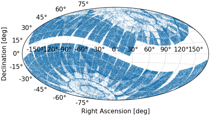
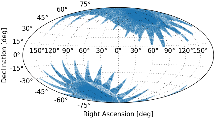
While the TESS Prime Mission (Sectors 1–26) observed a total of 232,705 unique stars in 2-min cadence ($\sim$20,000 stars observed per sector), we restrict our periodicity search to the 199,412 stars that are brighter than $T=14$ and are not severely blended with neighboring stars (CONTRATIO $<$ 0.2). We also only examine stars with physical parameters listed in the TIC, which does not include white dwarfs and many subdwarfs. We use the 2-min cadence time-series photometry that were processed by the Science Processing Operations Center (SPOC) pipeline (Jenkins et al., 2016), known as the Presearch Data Conditioning Simple Aperture Photometry (PDCSAP; Stumpe et al., 2012, 2014; Smith et al., 2012) light curves. The PDCSAP light curves are based on an optimal aperture extraction of the raw photometry that was detrended using co-trending basis vectors in order to correct for common instrument systematics. We apply additional post-processing to the light curves, including removing data that are flagged as being anomalous in quality, trimming any known and candidate planetary transit events, and removing outliers that are $>$5$\sigma$ from the RMS of the light curve. Transit events are removed using the reported orbital period and a transit duration that is 10% longer than that which is reported in the TESS Object of Interest (TOI) catalog (Guerrero et al., 2021). In addition to removing data that has been flagged as being anomalous quality by the pipeline, we remove observations between 1347.0–1349.8 TJD during which significant flux scatter is observed in most Sector 1 light curves due to a known spacecraft stability issue that is discussed in the TESS data release notes. This section of Sector 1 was the only set of data that we removed due to pervasive problems across many light curves.

2.2 Periodicity Search Tools

Stellar variability manifests in many forms, and can be periodic, semiperiodic, or stochastic. In this paper, we mostly concern ourselves with continuous periodic sinusoidal-like photometric variability. Such behavior is associated with stellar pulsations, rotational modulations due to starspots, and ellipsoidal variations in stellar binaries and can be detected with the Lomb-Scargle (LS) periodogram (Lomb, 1976; Scargle, 1982).

We compute the fast LS periodogram using the astropy.timeseries.LombScargle function and sampling at equally spaced frequencies that are 1.35 min^-1 apart, deliberately slightly oversampling the time series for maximal frequency resolution. The highest power peak in the periodogram is used to determine the most significant periodic signature of the light curve. The frequency, uncertainty, and significance (i.e., normalized power) of the most significant periodic signature are measured using a quadratic function fit to the highest power peak in the LS periodogram. The inverse of the frequency with the highest periodogram power is taken to represent the stellar variability period ($P=1/f$). A sinusoidal function is fit to the light curve and defined by

$$F(t) =A\cos\left[{\frac{2\pi}{P}(t-t_{0})}\right]\mathrm{,}$$ (1)

where $A$ is the amplitude of the sine wave, $t-t_{0}$ represents the time since the first maximum relative to each point in time, and $P$ is the period with the highest power from the LS periodogram. The reduced chi-squared, $\chi^{2}_{\nu}$, is used to determine the goodness-of-fit of the sinusoidal function.

In order to distinguish continuous periodic variability from more punctuated periodic variability, such as planetary transits and stellar eclipses, we also utilize the auto-correlation function (ACF). The ACF requires data that are equally spaced in time, therefore we interpolate any missing observations in time and set their relative fluxes to zero. The ACF is measured by correlating the interpolated data with itself and then smoothing the result using a Gaussian kernel. The lag time of the ACF that has the highest correlation (i.e., strongest peak) is fit with a quadratic function to identify the variability period, its uncertainty, and its significance (i.e., normalized power). To determine the goodness-of-fit for the ACF, the light curve is binned into 100 equally spaced points in phase space and a cubic interpolation of the binned points is used to represent the ACF model when calculating the $\chi_{\nu}^{2}$ of the ACF model compared to the light curve data.

2.3 Considerations of the TESS Photometry

There are several considerations that affect our periodogram search in accordance to the nature of the TESS photometry. In particular, continuous segments of observations take place over a single spacecraft orbit, the placement of each target on the CCD cameras changes between TESS sectors, and the spacecraft performs periodic adjustments in pointing that can introduce systematic noise into the photometry.

Continuous TESS observations occur during the majority of each spacecraft orbit, but there is a $\sim$1 day pause in observations when the spacecraft approaches perigee in order to downlink the data. Otherwise, observing conditions remain consistent over the course of two spacecraft orbits, which makes up the duration of a TESS sector ($\sim$27 days). Every TESS target is observed nearly continuously for at least one sector, such that we can search for repeatable signatures in the TESS light curves up to $\sim$13 days. However, periodic signatures that are measured to be closer to the 13-day limit are subject to greater uncertainties than those on shorter timescales.

There are 69,253 stars in our sample that have been observed in more than one sector of TESS photometry. Due to the observational design of the TESS mission, each TESS sector observes a different region of the sky such that any given star is not observed on the same part of the detector between sectors. The differing positions of the star on the detector introduces systematics into the time-series photometry that are typically not adequately removed with a simple normalization offset. Therefore, we choose to defer an investigation of long-period variability ($>$13 days) to a future work (Fetherolf et al. in prep.). In this work, we instead use these stars to understand the reliability of detecting stars that are astrophysically variable—as opposed to being caused by spacecraft systematics—in our catalog by ensuring that the same periodic signal for a given star can be recovered in different sectors (see Section 3.2).

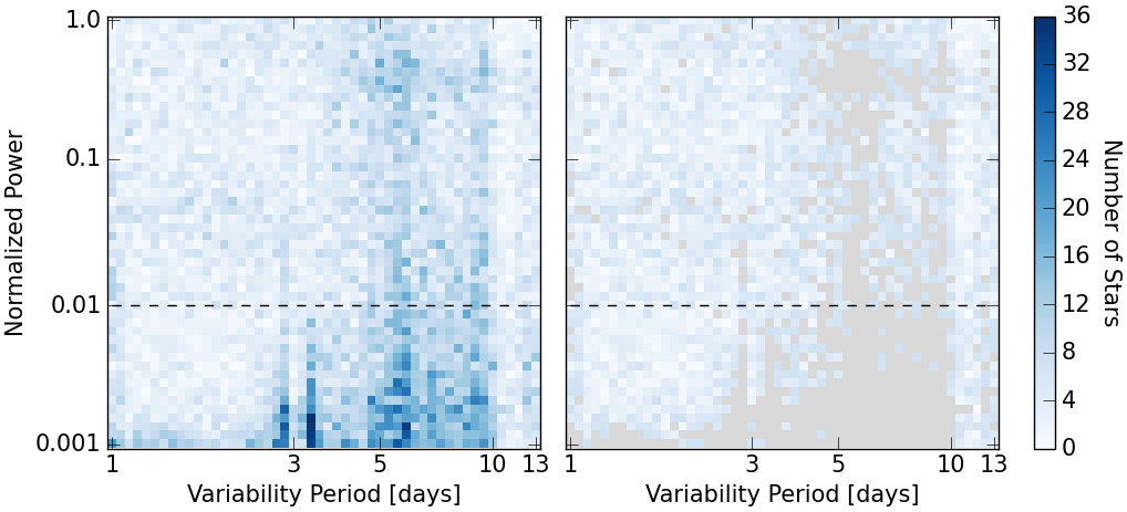
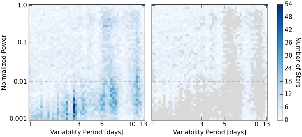
The spacecraft reaction wheels have their speeds reset (also known as “momentum dumps”) as frequently as every few days, which can cause periodic changes in the light curve that can masquerade as stellar variability. These systematic variations are not consistent between individual sectors (becoming less frequent over the mission duration), but they can occasionally be detected in the light curve at high Lomb-Scargle power in some cases. The left panels of Figure 2 show how the variability periods detected from the single sinusoidal model at 1–13 days are distributed in normalized power and period space for stars observed during TESS Sectors 5 and 17. There are several regions in the normalized power versus period space that contain a higher density of stars, but these periodicities would align between different TESS sectors if they were astrophysical in nature. In the interest of developing a stellar variability catalog of high confidence, we elect to remove any stars that fall in high-density regions in power versus period space for measured variability periods $>$1 day in each TESS sector at the cost of removing a few real variable stars from the catalog (see Section 2.4 and right panels of Figure 2).

Figure 2: Normalized LS power versus the most significant photometric periodicity detected from the light curves for stars that were observed during TESS Sectors 5 (top) and 17 (bottom). The left panels show the density of stars in power-period space. The right panels show in gray which bins were deemed high density ($>$7 stars), such that the stars were removed from the catalog. Stars that fall in high density regions of power-period space are likely exhibiting periodic modulations in their light curves that can be attributed to instrument systematics. The horizontal dashed line shows the normalized LS power cut that is applied to the final catalog (Tables 1–3).

2.4 Variability Search

Figure 3: A flowchart that summarizes our variability search algorithm, with the direction of flow being indicated by black (always), green (only when True), or red (only when False) arrows. Starting from the stars observed during the TESS Prime Mission, we first remove stars that are faint ($T_{\mathrm{mag}}>14$ mag) or subject to significant blending (CONTRATIO $>$ 0.2). We then search for periodic signatures at 0.01–1.5 and 1–13 days in each individual sector of TESS photometry. Several tests are preformed to determine significance of variability that is best fit with a single sinusoidal model (see Section 2.4). Stars that make it into one of the “Variable” categories are included in Tables 1–3.

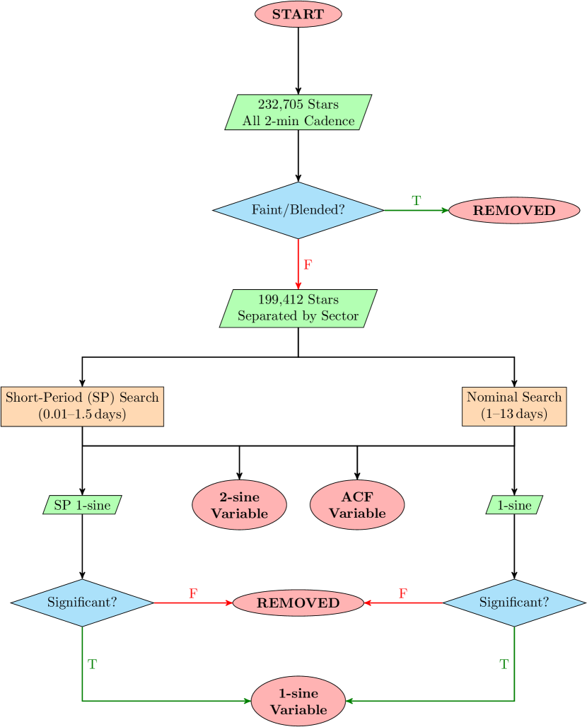
We perform a periodogram search on 199,412 unique stars, which comprises approximately half a million light curves that were obtained in TESS Sectors 1–26. Our periodogram search includes two distinct period ranges at 0.01–1.5 days and 1–13 days. Figure 3 shows the overall flow of our periodogram search, where stars that we identify as significantly variable are best characterized by either a single-sinusoidal function (1-sine Variable), a double-sinusoidal function (2-sine Variable), or the ACF (ACF Variable).

Our default model for the light curve is a single sinusoidal fit, but a double-sinusoidal function fit is also performed when the second-highest peak in the LS periodogram has a normalized power greater than 0.1. The double-sinusoidal fit is accepted as a better model than the single-sinusoidal fit to the light curve variations if there is at least a 25% improvement in the $\chi_{\nu}^{2}$. The ACF fit is performed when both the single- and double-sinusoidal models are poorly fit ($\chi_{\nu}^{2}>100$) to the light curve. The ACF is accepted as a better model if the strongest correlation value is greater than 0.5 and the $\chi_{\nu}^{2}$ improves compared to the sinusoidal models. A star that is best fit with either a double-sinusoidal model or the ACF is considered significantly variable by default, the purity of which is further explored in Section 3.2. The values for the normalized power cutoffs and $\chi_{\nu}^{2}$ improvement were determined through visual inspection of the light curve fits for a preliminary sample of stars.

If a star that passes the initial periodogram search and is not identified as significantly variable with a double-sinusoidal function or the ACF, then it is subject to further vetting after assuming the single-sinusoidal fit to be the best model. First, a separate short-period variability search (0.01–1.5 days) is performed and used to identify significant variability on short timescales ($<$1.1 days) when the normalized power is $>$0.01 normalized LS power. Several vetting steps are then applied to remove systematic or long-period ($>$13 days) variability from the nominal periodogram search at 1–13 days, with the first being a minimum threshold normalized LS power of 0.01. To retain high purity in the variability catalog, we remove stars that fall in high-density regions in power-period space for variability periods measured to be greater than 1 day (see Section 2.3 and Figure 2), where variability is likely due to spacecraft systematics. High-density regions are determined by binning the log power and log period into 50 equally spaced bins (power $=$ 0.001–1.0; $P=$ 1–13 days), and stars whose variability properties fall within bins that contain seven or more total stars are considered to be spuriously variable—although we reiterate that some real variable stars will be removed during this step. Figure 2 shows examples from two sectors of the power-period distribution patterns in which stars are removed from our catalog based on the high density in power-period space for Sectors 5 and 17, where different patterns in power-period space can be seen. However, most of the stars that are inevitably removed from the catalog based on the high-density regions in power-period space tend to fall below our minimum normalized LS power threshold of 0.01. Stars that are variable on timescales longer than that which can be properly constrained by the TESS single-sector photometry ($\gg$13 days), or are indistinguishable from uncorrected systematics on these timescales, are identified via two methods and removed from our variability catalog: 1) Stars that exhibit a maximum power in their LS periodogram at the upper limit of the period range searched (i.e., 13 days) are assumed to exhibit variability at $\gtrsim$13 days, which is beyond our sensitivity limit for the variability period. 2) We perform a linear fit to each light curve; if the $\chi_{\nu}^{2}$ of the linear fit is better than that of the sinusoidal or ACF models, we consider the star to have a long-term trend. Overall, stars that exhibit single-sinusoidal variability are considered significantly variable and, thus, are retained in our variability catalog if they are not caught by the filters for being spuriously variable and if they do not exhibit long-term trends.

Stars that were observed in multiple TESS sectors may be detected as significantly variable in more than one sector. However, the variability period may not match between all sectors. It may be that the detected periodicity in one sector is half or twice that of another sector, the photometric variability for a given sector may be dominated by periodic momentum dumps of the spacecraft, or the star may be exhibiting variability that changes in period or amplitude over time. For the variability catalog reported in this work, we provide only the results from a single sector of TESS photometry. The TESS sector from which we report the periodogram results for a given star is based on first prioritizing any variability that is best fit by an ACF or double-sinusoidal model, then choosing the periodogram result with the highest normalized power.

Table 1: Light Curve Fitting and Stellar Properties of Single-Sinusoidal Variables

TIC	Sector	$P_{\mathrm{var}}$	power	$A$	$T_{0}$	$\chi^{2}_{\nu}$	RMS	$T_{\mathrm{mag}}$	$T_{\mathrm{eff}}$	$R_{*}$	$L_{*}$
		(days)		(ppm)	(BTJD)		(ppm)		(K)	(R⊙)	(L⊙)
355235442	9	$1.225\pm 0.024$	0.999	43096	1543.778	5.65	30751	10.15	5266	1.02	0.72
361948797	16	$9.485\pm 1.361$	0.999	52113	1743.029	6.89	37109	8.77	14618	—	—
285651536	12	$12.365\pm 2.394$	0.998	22679	1625.519	6.07	16823	7.85	—	—	—
29953651	9	$1.472\pm 0.033$	0.995	20919	1544.337	11.92	14845	8.10	—	—	—
441807438	21	$1.135\pm 0.018$	0.995	33715	1871.116	19.43	23917	8.81	5181	1.22	0.97
127256815	7	$1.313\pm 0.027$	0.994	26086	1491.655	9.46	18674	8.95	13833	—	—
47985275	6	$1.111\pm 0.021$	0.993	16295	1465.957	4.15	11605	9.37	12081	—	—
303860976	11	$1.275\pm 0.025$	0.993	6953	1596.913	2.62	4993	7.97	10237	3.83	144.53
117765777	6	$1.101\pm 0.021$	0.992	31558	1465.491	78.11	22488	7.91	11345	3.00	134.18
401481773	10	$8.580\pm 1.209$	0.992	24077	1577.481	9.97	17740	8.63	—	—	—

is available in the machine-readable format.

Note. — The 10 stars with the highest LS normalized power are listed here as a reference, but the complete table with several additional columns of information

Table 2: Light Curve Fitting and Stellar Properties of Double-Sinusoidal Variables

TIC	Sector	$P_{\mathrm{var}}$	power	$A$	$T_{0}$	$\chi^{2}_{\nu}$	RMS	$T_{\mathrm{mag}}$	$T_{\mathrm{eff}}$	$R_{*}$	$L_{*}$
		(days)		(ppm)	(BTJD)		(ppm)		(K)	(R⊙)	(L⊙)
56980355	8	$4.490\pm 0.281$	0.984	35938	1520.424	16.25	25262	9.08	9684	4.95	193.51
		$6.045\pm 0.487$	0.316	3387	1518.653
140797524	8	$9.576\pm 1.287$	0.979	87883	1525.411	904.94	61352	7.24	4691	8.67	32.69
		$6.216\pm 0.516$	0.332	7859	1519.354
455000299	11	$7.911\pm 0.899$	0.977	30308	1596.905	7.18	21797	10.09	4397	1.18	0.47
		$5.220\pm 0.398$	0.417	3457	1598.956
33298241	7	$11.784\pm 2.262$	0.968	47926	1499.506	86.60	34356	8.88	10636	4.02	185.68
		$6.944\pm 0.546$	0.143	4868	1491.729
291366757	12	$8.328\pm 1.009$	0.965	30518	1632.860	178.56	21593	7.18	8231	3.56	52.26
		$5.580\pm 0.379$	0.210	3800	1628.350
255585244	7	$11.819\pm 2.360$	0.965	36199	1502.757	5.06	25681	9.67	—	—	—
		$6.940\pm 0.550$	0.210	5036	1492.010
202414513	17	$12.515\pm 2.167$	0.964	16514	1769.312	9.51	10897	8.53	3550	95.10	1289.69
		$6.958\pm 0.656$	0.449	1417	1771.497
258908663	11	$6.147\pm 0.560$	0.957	52026	1600.852	6.22	36753	11.62	3731	0.88	0.13
		$10.151\pm 1.458$	0.383	11196	1600.146
57065604	9	$11.338\pm 2.502$	0.953	57539	1550.353	547.86	41710	7.99	11179	2.52	88.87
		$6.693\pm 0.524$	0.273	7994	1549.570
280161519	14	$12.859\pm 2.680$	0.951	12086	1689.719	14.75	8704	8.12	3672	59.03	568.85
		$7.703\pm 0.572$	0.154	1533	1687.899

is available in the machine-readable format.

Note. — The 10 stars with the highest LS normalized power are listed here as a reference, but the complete table with several additional columns of information

Table 3: Light Curve Fitting and Stellar Properties of ACF Variables

TIC	Sector	$P_{\mathrm{var}}$	correlation	$A$	$T_{0}$	$\chi^{2}_{\nu}$	RMS	$T_{\mathrm{mag}}$	$T_{\mathrm{eff}}$	$R_{*}$	$L_{*}$
		(days)		(ppm)	(BTJD)		(ppm)		(K)	(R⊙)	(L⊙)
451949522	10	$0.454\pm 0.002$	0.937	105168	1569.842	5.28	36430	8.94	4962	1.77	1.70
162432383	10	$0.324\pm 0.002$	0.935	12114	1569.524	70.84	4800	8.07	7308	1.38	4.86
41170667	9	$0.487\pm 0.002$	0.932	200327	1543.618	14.06	69559	10.30	6853	3.51	24.41
24662304	6	$0.545\pm 0.007$	0.932	13671	1465.473	829.76	5922	6.29	—	—	—
285413207	7	$0.638\pm 0.003$	0.931	44123	1492.088	5.75	16092	9.96	6254	1.15	1.81
43216747	22	$0.438\pm 0.002$	0.930	99613	1899.351	5.43	35717	10.35	5083	1.10	0.73
132764448	7	$0.418\pm 0.001$	0.930	29187	1491.636	3.41	10413	9.34	4612	0.96	0.38
157212164	7	$0.572\pm 0.002$	0.929	93374	1491.733	6.98	32852	10.51	5647	0.89	0.73
424721218	20	$0.388\pm 0.001$	0.929	334262	1842.409	2.55	119979	11.64	7165	5.05	60.44
140132301	9	$0.329\pm 0.001$	0.928	201079	1543.415	69.62	71698	9.32	—	—	—

Note. — The 10 stars with the highest correlation value are listed here as a reference, but the complete table with several additional columns of information is available in the machine-readable format.

3 Results

3.1 Variability Catalog

Tables 1–3 list the 68,497 stars that are significantly variable when described by a simple sinusoidal function (30,370 stars with $>$0.1 normalized power), 10,887 stars that exhibit double-sinusoidal variability, and 4,662 stars that are otherwise strictly periodic and best characterized with the ACF, for a total of 84,046 unique stars that are included in the variability catalog as a whole. The variability period ($P_{\mathrm{var}}$) and normalized power (or correlation) are determined from the LS periodogram (or ACF). The amplitude ($A$) and time of maximum flux ($T_{0}$) of the light curve modulations—and the corresponding reduced chi-squared statistic ($\chi_{\nu}^{2}$)—are measured from the best-fit single- or double-sinusoidal function. The TESS magnitude ($T_{\mathrm{mag}}$), stellar effective temperature ($T_{\mathrm{eff}}$), and stellar radius ($R_{*}$) are taken from the TICv8 catalog (Stassun et al., 2018, 2019) when available, and we calculate stellar luminosities ($L_{*}$) using the reported radii and temperatures. The online version of the machine-readable catalog includes several additional informational columns including uncertainties from the sinusoidal fitting, metrics for goodness-of-fit, and all of the contents of the TICv8 catalog for these stars (including coordinates). Table 1, in particular, includes variability that was detected with at least 0.01 normalized power ($\sim$68,000 stars), but we hold the highest confidence in the variability of stars with $>$0.1 normalized power ($\sim$30,000 stars). The figures and results that follow only include variable stars that were detected with at least 0.1 normalized power (45,919 stars). Tables 1–3 are available in the machine-readable format and figures showing the light curve, LS periodogram, and phase-folded light curve (e.g., see Figures 4–6) for each star in the variability catalog are available as a High-Level Science Product (HLSP) on MAST: http://dx.doi.org/10.17909/f8pz-vj63 (catalog DOI: 10.17909/f8pz-vj63).

Our default model assumes sinusoidal variability, which will generally encapsulate rotational variability. Figure 4 shows three examples of periodic variability that are best characterized by a single-sinusoidal function. Light curve modulations that are characterized by a single periodic signal can represent a broad range of stellar activity, including rotational variations caused by starspot activity, a dominant pulsation, or overcontact binaries. The examples shown in Figure 4 showcase three examples of rotational and/or pulsational modulations, including an F star that is hotter than the Kraft break (top row; TIC 99971569), an M dwarf star that has not spun down over time due to its fully convective interior (center row; TIC 220523369), and a giant star exhibiting more quasi-periodic rotation (bottom row; TIC 97423262).

Figure 4: Single sector light curve (left column), periodogram (center column), and phase-folded light curve (right column) for 3 examples of stars that are best characterized by a single-sinusoidal function. The black points in the right panels show the medians of 100 bins for the phase curve. The red curve represents the best-fit sinusoidal function and the blue triangles denote spacecraft momentum dump timings. The examples shown include a quickly rotating F star (top row), an M dwarf with a fully convective interior (center row), and a red giant star (bottom row).

Some stars exhibit multiple periodicities in their light curves, thus being better characterized by a double-sinusoidal function. Examples of more complex light curves that are best characterized by a double-sinusoidal function are shown in Figure 5. Multi-periodic variations in stars could be attributed to pulsations or differential stellar rotation. The light curves shown in Figure 5 show examples of a $\delta$ Scuti pulsator (top row; TIC 70657495), a rotating F star that is cooler than the Kraft break (center row; TIC 468838146), and a giant star with two close periodicities (bottom row; TIC 71374409).

Figure 5: Same as Figure 4, except for stars that are best characterized by a double-sinusoidal function. The right panel shows the phase-folded light curve for the two periodicities that are identified. The examples shown include a $\delta$ Scuti pulsator (top row), an F star with a harmonic rotation (center row), and a giant star (bottom row).

Light curves that are significantly periodic in nature, but are not sinusoidal in shape, are best characterized using the ACF. Finally, we show examples of light curves that exhibit strictly periodic variability that is not necessarily sinusoidal in shape in Figure 6, which are best characterized by the ACF. These light curves typically represent short-period ($<$11 days) eclipsing binary systems with V-shaped eclipses, but also can include strictly periodic non-sinusoidal rotational variability. The examples shown in Figure 6 represent an RR Lyrae variable star (top row; TIC 393702163), an eclipsing binary with a V-shaped eclipse and strong Doppler boosting variations (center row; TIC 279254042), and a flat-bottomed eclipsing binary with strong ellipsoidal modulations (bottom row; TIC 450089997).

Figure 6: Same as Figure 4, except for stars that are best characterized by an ACF. The center panel shows the correlation over the range of searched variability periods. The red curve represents an interpolation between each median binned point in the phase curve. The examples shown include an RR Lyrae variable star (top row), an eclipsing binary with a V-shaped eclipse (center row), and an eclipsing binary with ellipsoidal modulations (bottom row).

3.2 Catalog Reliability

We can characterize the reliability of our catalog by examining stars observed in more than one sector. We compare the periodogram search results for the stars across individual sectors to see whether the periodicity properties are consistent between sectors. As stated in Section 2.4, we select a single TESS sector for reporting the variability analysis results in our catalog (Tables 1–3) that is based on the periodicity with the highest normalized power. This selected sector is used as the reference when comparing variability analyses from multiple TESS sectors.

There are 19,118 stars that are best characterized by our default model (single-sinusoidal function) and were observed in multiple TESS sectors. For 13,968 stars, we find that the periodicity measured from the selected sector agrees within 10% of either: 1) the periodicity detected from any other individual sector of photometry; 2) twice or half the periodicity detected from other sectors of photometry; 3) the average periodicity measured from each of the individual sectors; or 4) the average periodicity after removing the largest outlier when the star was observed in three or more TESS sectors. Stars whose periodic signatures are not in agreement between multiple sectors may still be astrophysically variable, but could be affected by differential spot rotation or poor photometric detrending in one of the sectors. Overall, there are 5,150 stars in our single-sinusoidal variability catalog that were observed in multiple sectors but we cannot confirm their astrophysical nature, suggesting a possible 27% degree of contamination in the single-sinusoidal variability catalog (Table 1) by non-variable stars. The catalog contains a list of stars with periodicities that have $>$0.01 normalized power, but we hold higher confidence that the stars with $>$0.1 normalized power are intrinsically variable since only 12% of these stars are unconfirmed from their multiple sectors of photometry.

There are 3,907 stars that are observed in multiple TESS sectors and best characterized by a double-sinusoidal function. We find that, for all but 41 stars, at least one of the two periodicities identified from the selected sector variability analysis is within 10% of one of the two periodicities identified in other sectors characterized by a double-sinusoidal function. There are only 12 stars that have periodicities that are inconsistent with other sectors beyond 15% period variance, but after visual inspection of their light curves we find that they are all consistent with being intrinsically variable in nature with their inconsistent periodicities between TESS sectors being attributed to differential rotation (i.e., several close significant periodicities). Overall, we infer with high confidence that all stars identified as exhibiting a double-sinusoidal signature in their light curve are truly variable in nature—even when identified using only a single sector of TESS photometry (see Table 2).

There are 1,900 stars that are observed in multiple TESS sectors and are periodic, but not necessarily sinusoidal in nature, and are thus best characterized by an ACF. Stars that are best characterized by an ACF in at least one TESS sector are typically consistent with other ACF periodicities available in other sectors within 10% of the period. There are 7 stars that have inconsistent results, but are visually examined and found that they could all equally be described by a double-sinusoidal function, with several significant periodicities that are not necessarily harmonics of each other. Given that these few exceptions are visually confirmed as being significantly variable in nature, we infer that all stars with light curves that are best fit with an ACF—including those that were observed in only a single sector of TESS photometry—are confirmed as being truly variable in nature with high confidence (see Table 3).

The potential contamination of the variability catalog by non-variable stars is primarily dominated by stars that are best characterized by a single-sinusoidal function. We split the contamination level of the stars identified by a single-sinusoidal function into two groups based on whether they have greater than or less than 0.1 normalized power. There are 38,127 stars with $<$0.1 normalized power in the variability catalog, where we estimate a maximum of 27% contamination by non-variables. The 30,370 stars that are characterized by a single-sinusoidal function and have $>$0.1 normalized power are estimated to be 12% contaminated by non-variable stars. Stars that are best characterized by either a double-sinusoidal function or an ACF are assumed to all be true variable stars. Overall, we estimate that the variability catalog as a whole is at most 21% contaminated by non-variable stars.

4 Discussion

4.1 Demographics of Variable Stars

The analysis presented here makes use of the TESS time-series photometry and the estimated stellar properties from the TICv8. The photometric analysis only considers periodic variability in the TESS bandpass that can be detected using the Lomb-Scargle periodogram and the auto-correlation function. These diagnostics are not sufficient for a detailed demographic study linking the morphology of periodic variability to the specific mechanisms of stellar structure and evolution. They do not incorporate many other ways to characterize stellar variability, such as stochastic (nonperiodic) variability, chromatic changes, spectroscopic variability, or other measures of changing flux. Nevertheless, we can extract information from this analysis that tells us about broad classes of variability by visually exploring the summary figures produced through our analysis (e.g., Figures 4–6) using the FilterGraph data visualization tool. We first consider the distribution of variability across the Hertzsprung-Russell diagram (HRD), and we then explore the relationship between periodicity and stellar luminosity.

Figure 7: Hertzsprung-Russell diagram of stars that are identified as significantly variable, and thus are included in the variability catalog (Tables 1–3). The points are colored by the measured variability period. Luminosities are calculated from the effective temperatures and stellar radii available in the TICv8 catalog (Stassun et al., 2018, 2019).

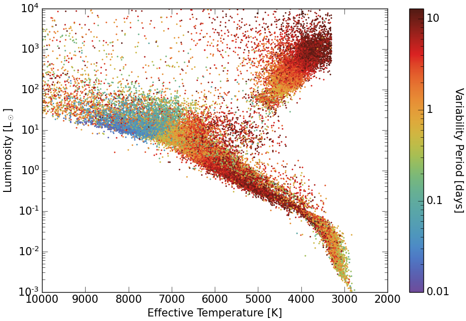
Figure 7 shows the stars in the variability catalog on the HRD colored by their measured variability periods. The figure includes the subset of variable stars that were best characterized by a single-sinusoidal model (Table 1), double-sinusoidal model (Table 2), or ACF (Table 3). The location of stars on the HRD is significantly correlated with their measured variability period, which supports the expectation that the variability in these stars is primarily driven by starspot rotation and pulsations. We can describe the mechanisms for variability by connecting the different regions on the HRD with the variability periods measured from this work and examples of their observed light curves (e.g., Figures 4–6).

The stars with the longest variability periods are on the red giant branch and single FGK dwarf stars, which tend to have slower rotation periods as they age (Irwin & Bouvier, 2009; Meibom et al., 2009; van Saders & Pinsonneault, 2013; Angus et al., 2019). Low-mass M dwarf stars ($<3500$ K), on the other hand, have fully convective interiors such that they do not spin down as quickly over time and maintain generally short rotation periods ($<$1 day; Chabrier & Baraffe, 1997; Wright et al., 2011, 2018; Astudillo-Defru et al., 2017; Newton et al., 2017). The shortest variability periods are found in OBAF oscillating stars, which experience multiple modes of pulsations that reveal information about their internal structures (Gaia Collaboration et al., 2022; Kurtz, 2022). A few stars in this sample also outline the binary sequence (e.g., Gaia Collaboration et al., 2018, 2019), which is offset from the main sequence towards higher luminosities and was typically better characterized by an ACF with shorter variability periods. For stars characterized by an ACF, the main sequence tends to be dominated by eclipsing binaries, overcontact binaries, other tidally locked binaries, and fast rotating young main sequence stars, with just a few stars dominated by longer period starspot rotational modulations on the lower luminosity edge of the main sequence. The red giant branch includes a mix of intrinsic variables and eclipsing binaries. There are also a few variable stars identified along the instability strip—including those that are consistent with being RR Lyrae or Cepheid variables.

Finally, we highlight the existence of what appears to be a prominent sub-subgiant population above the binary main-sequence and below the sub-giant branch. Sub-subgiant (SSG) stars have been recognized as likely representing unusual stellar evolution pathways ever since their initial detection as anomalies in the color-magnitude diagrams (CMDs) of some open clusters (see, e.g., Mathieu et al., 2003, and references therein). Subsequent studies of SSGs in clusters have proffered several possible interpretations for these systems: mass transfer in a binary system, collision of two main sequence stars, mass loss of subgiant envelopes through dynamical encounters, and reduced luminosity due to the strong surface coverage of magnetic starspots (see, e.g., Leiner et al., 2017). Some recent works have concluded that mass transfer and dynamical formation pathways are disfavored based on the small numbers of SSGs in open clusters, preferring instead the strong starspot interpretation (e.g., Gosnell et al., 2022). However, attempts to identify and characterize the broader SSG population in the field have only very recently begun (Leiner et al., 2022). Thus, the large population of apparent SSGs in the field identified in Figure 7 could be an opportunity to make substantial new progress in understanding these enigmatic systems.

Figures 8–10 show the period-luminosity relationship for the stars that are included in the stellar variability catalog. Figure 8, in particular, highlights which stars are best characterized by a single-sinusoidal model (black points), double-sinusoidal model (blue points), or ACF (orange points). Figure 9 is colored by the effective temperature and includes labels for several known astrophysical features, and Figure 10 is colored by the measured variability amplitude from their light curves to emphasize how the strength of the photometric variations can be used to differentiate between different types of stellar variability.

The distribution of variable stars in the period–luminosity diagram is similar between the stars that were best characterized with a single- or double-sinusoidal function. The OBAF main sequence stars show a positive correlation between their luminosities and short-period oscillations ($\lesssim$0.2 days; Gaia Collaboration et al., 2022; Kurtz, 2022), and we attribute the bimodal clustering of this group to ambiguous identification between the first two harmonics of oscillations that exhibit similar strength in LS normalized power. The discontinuity at $\sim$4 L_⊙ luminosity is attributed to the Kraft break ($\sim$6200 K; Kraft, 1967), where cooler stars tend to rotate more slowly as magnetized stellar winds remove angular momentum from the star. There is also a positive linear relationship between luminosity and variability period for stars on the evolved giant branch ($\gtrsim$100 L_⊙), which is consistent with asteroseismic studies of red giants (Huber et al., 2011; Mosser et al., 2012). The primary difference between the stars best characterized with a single-sinusoidal versus double-sinusoidal function can be seen in the giant stars, where multiple periodicities (i.e., 2-Sine) shorter than $\sim$1.5 days are not observed in giant stars. The transition from single-sinusoidal to double-sinusoidal variability towards higher luminosity giant stars is in contrast with previous studies that have found instead that higher luminosity giants tend to pulsate with fewer distinct modes than low-luminosity giant stars (Stello et al., 2014; Yu et al., 2020). However, this discrepancy may be caused by a detection bias in our catalog since lower luminosity giants tend to have smaller oscillation amplitudes.

Figure 8: Calculated stellar luminosities versus the measured variability periods of stars that are identified as significantly variable, and thus are included in the variability catalog (Tables 1–3). The points are colored by whether their light curves were best characterized by a single-sinusoidal function (black points), double-sinusoidal function (blue points), or ACF (orange points). Luminosities are calculated from the effective temperatures and stellar radii available in the TICv8 catalog (Stassun et al., 2018, 2019).

Figure 9: Same as Figure 8, but the points are colored by their effective temperatures. Several known astrophysical relationships are highlighted and labeled with faded ellipses.

Figure 10: Same as Figure 8, but the points are colored by the variability amplitude measured from their representative light curves.

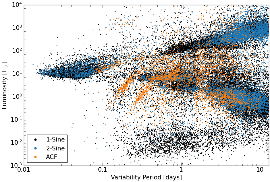
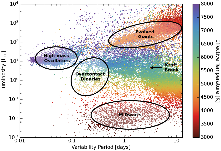
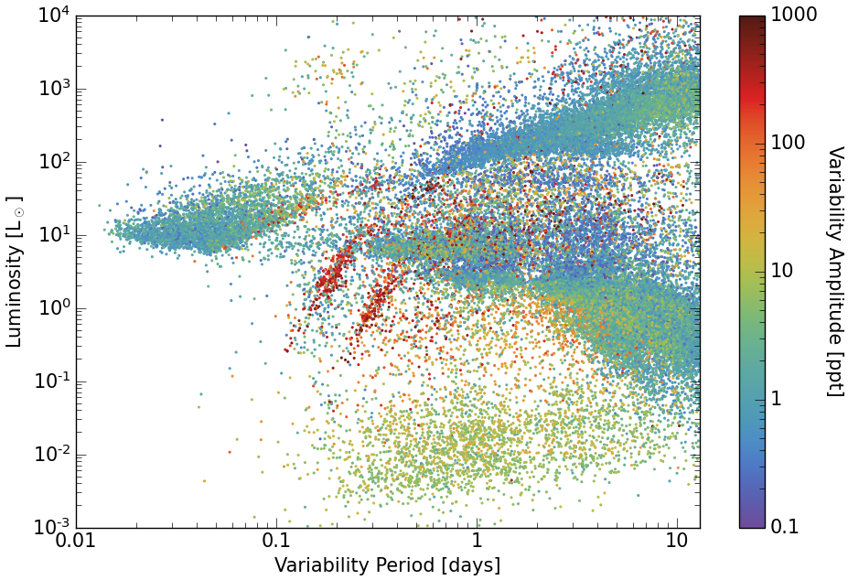
The period-luminosity relationship for stars characterized with an ACF (orange points in Figure 8) is vastly different when compared to the stars with variations that are more sinusoidal in nature (black and blue points). Stars with higher amplitude variations (redder points in Figure 10) tend to be eclipsing or overcontact binaries. In particular, the period-luminosity relationship for overcontact binaries can be seen twice, where the shorter period relationship is half the binary orbital period. In order to avoid incorrectly shifting non-binary periods, we choose to not artificially double the periods for the stars that fall along the shorter period overcontact binary sequence. The linear relationship at higher luminosities ($\gtrsim$5 L_⊙) with periods ranging between $\sim$0.01–0.2 days represents the period-luminosity relationship for $\delta$ Scuti stars (King, 1991; Antoci et al., 2019; Ziaali et al., 2019; Barac et al., 2022; Kurtz, 2022). There is also a separation in luminosity ($\sim$4 L_⊙) for stars with lower amplitude variations that can be attributed to the Kraft break.

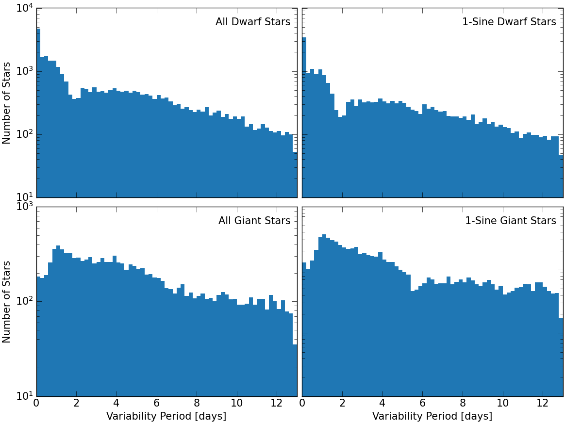
The left panels of Figure 11 shows histograms of the variability periods measured for all dwarf and giant stars in the variability catalog, where we assume the identification of dwarf and giant stars using the LUMCLASS flag in the TICv8 catalog (Stassun et al., 2018, 2019). There are significantly fewer dwarf stars that exhibit variations on timescales of 1.5–2 days, which is not necessarily related to the Kraft break since these rotation periods are also uncommon for M dwarf stars (see Figure 9). If the dearth of variability at 1.5–2 days were caused by a systematic effect, then the drop in occurrence would be observable in both the dwarf and giant stars. On the contrary, the drop in variable stars at 1.5–2 days only occurs in dwarf stars even when only the subset of stars that were best fit by a single-sinusoidal function are considered (right panels; Section 2.3). Kounkel et al. (2022) suggested that binaries amount FGK-type stars with periods faster than $\sim$2 days, and M-type stars with periods faster than $\sim$1.5 days are predominately binaries that are possibly undergoing tidal interactions. Furthermore, the lack of $\sim$2 day periodicities spans over 4 orders of magnitude in luminosity, including M dwarfs, which suggest that it is could be related to binarity rather than pulsations. However, we leave an in-depth investigation in the binary occurrence rate in FGKM stars near variability periods of 1.5–2 days to a future work.

In the right panels of Figure 11 we observe fewer variable stars at 5–6 days for both dwarfs and giants, which is in contrast to Holcomb et al. (2022) where they identified an overdensity of rotational variables at $\sim$5 days. However, they suspected that their observed overdensity of variable stars at $\sim$5 days could be related to uncorrected systematics in the TESS PDCSAP photometry. This interpretation is consistent with how we removed variable stars from the variability catalog that were best be characterized by a single-sinusoidal function but could be attributed to spacecraft systematics—including some stars that are truly variable at 5–6 days (see Section 2.3).

Figure 11: Histograms of the measured variability periods for all (left panels) dwarf (top panels) and giant (bottom panels) stars and the subset of stars best characterized by a single-sinusoidal function (right panels). Both dwarf and giant stars characterized by a single-sinusoidal function have fewer variables at $\sim$5–6 days due to the removal of true intrinsic variables when accounting for TESS systematics (see Section 2.3). However, only dwarf stars show fewer variable stars at $\sim$1.5–2 days.

4.2 Demographic Comparisons to Similar Work

Projects similar to this paper have been undertaken using photometric data from other sky surveys, as described in Section 1. The observational and methodological heterogeneity of these surveys makes it hard to directly compare their bulk variability results. However, we can qualitatively compare the results from this study to those of the two of the most similar surveys: the exploration of variable stars across the HRD using Gaia data in Gaia Collaboration et al. (2019), and the search for periodic stellar variability in data from the ground-based NGTS survey in Briegal et al. (2022). The observational properties of both surveys have some overlap with the stellar population observed by TESS, and we intend to do direct star-by-star comparisons with those results in future work (see discussion in Section 4.4).

In Gaia Collaboration et al. (2019), the authors examine the position of variable star classes on the HRD, separated by the various intrinsic and extrinsic types of known stellar variability. They compile a large set of known variable stars from various published sources and locate them on the HRD using Gaia colors and magnitudes, and also conduct a limited exploration of stellar variables using Gaia photometry, considering only the amplitude (the interquartile range) of the Gaia $G$-band light curves. They identify regions of the HRD with a greater incidence of variability (see their Fig. 8), and also differences in typical variability amplitude across the HRD (their Fig. 9). Briegal et al. (2022) conduct a general search for periodic variability in their lightcurves, which cover a set of fields around the sky, each observed for an average of 141 nights across an average time baseline of 218 days. Their variability search method shares some broad similarities to ours, while also being careful to remove the systematic trends that arise in wide-field ground based photometric observing. They also plot their variability detections across a CMD using Gaia magnitudes.

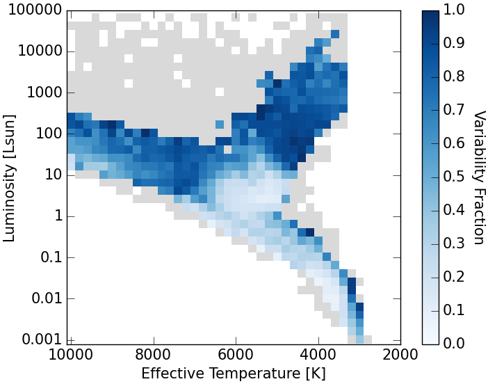
We can examine some of the variability distributions across the HRD between the studies. This comparison is only qualitative and approximate, since the Gaia and NGTS analyses use CMDs whereas we are plotting physical properties in an HRD. Also, the selection of targets for TESS 2-min cadence observations was motivated by the search for transiting planets and not a broad sample of stars in a magnitude-limited way, which will certainly lead to selection biases in the numerical results. Gaia observes deeper than TESS to fainter stars, and over a longer time frame (22 months), with fewer individual epochs of observation (of order 20 or more observations). NGTS observes a more similar set of stars in apparent magnitude, and over a time baseline more similar to Gaia, but with a number of epochs more similar to TESS. On the other hand, TESS light curves have much greater photometric precision and duty cycles than either of the other surveys. Nevertheless, we can still qualitatively compare our overall distributions to those in these other two papers.

We plot the fraction of stars that we identify as variable across the HRD in Figure 12. Similar to Fig. 8 from Gaia Collaboration et al. (2019) and Figs. 3a and 7 in Briegal et al. (2022), we show higher rates of variability—especially with short periods—for the hot stars of the upper main sequence, and also along the top edge of the lower main sequence, which includes the binary sequence. The increased variability fraction for hotter stars on the upper main sequence is consistent with observations of the $\delta$ Scuti instability strip (Murphy et al., 2019). We do not show the high rates of variability at the upper part of the red giant branch due to the limited time span of the single-sector TESS observations in this analysis. We do show high rates of variability on the lower part of the giant branch, but the comparison of an HRD with a CMD, and varying timescales of variability probed between the different surveys make that point difficult to verify.

Figure 12: The fraction of stars that are determined to be significantly variable across the HRD, with normalized power cutoffs of 0.01 (left) and 0.1 (right). The gray bins indicate areas of low completeness ($<$10 stars). Note the increased fractions of variable stars at the upper edge of the binary main-sequence as well as among the sub-subgiant population.

Figure 13: Same as Figure 7, but the points are colored by the measured variability amplitude from the light curves. Note the gradient of increasing variability amplitude with increased displacement above the main-sequence; these are evidently binary stars on the binary main-sequence. Interestingly, the sub-subgiant population exhibits a heterogeneity of variabilty amplitudes.

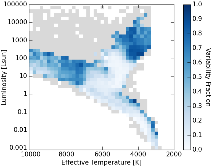
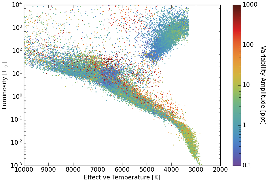
We can look at the distribution of variability amplitude between Figure 13 and Fig. 9 in Gaia Collaboration et al. (2019). We show the same increase in typical variability amplitude for stars on the upper edge of the main sequence, around the binary sequence. We see a gap in variability between the main sequence and the upper end of the giant branch, although the correspondence between the gaps in the two plots around the subgiant and lower giant branch regimes is not well defined. Above the part of the main sequence where the subgiant branch emerges, we find a number of very high-amplitude variables, which turn out to be classical pulsators in the instability strip. We do not see the high amplitudes among the red giant stars in the TESS data due to the limited time frame of the current analysis, although once we incorporate multi-sector TESS data in future work the red giant high-amplitude, long-period variability should become more apparent.

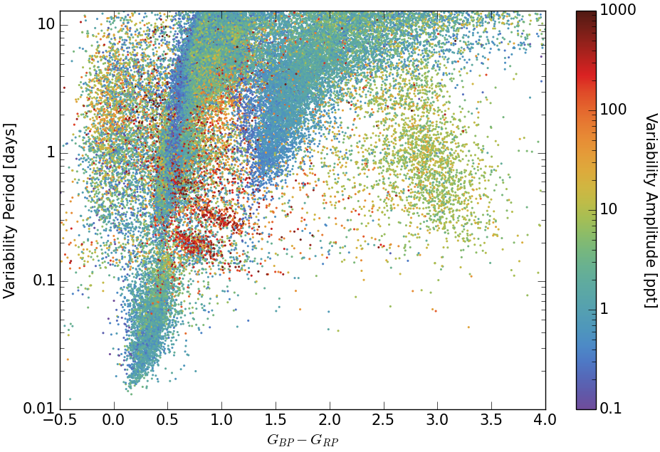
While Gaia Collaboration et al. (2019) did not include an investigation of periodic variability, Briegal et al. (2022) does compare the periodicity of their variables to the colors of the stars in a manner similar to our analysis throughout Section 4.1. We make a direct comparison to the period-color distribution of Fig. 8 from Briegal et al. (2022) in Figure 14, where we show our measured variability periods versus Gaia $G_{BP}$ and $G_{RP}$, and color the points by the amplitude of their variability. We see a similar distribution to the figure in Briegal et al. (2022), with a gradual trend towards longer variability periods for redder stars. Also seen at periodicities between 0.1 and 0.5 days are two populations of variables with the opposite trends with color, which we visually confirm as representing the overcontact binaries. In general, the upper population represents those stars identified at the correct orbital period, while the lower population represents those identified at half the true period, as noted also in Briegal et al. (2022).

Figure 14: Variability period versus Gaia $G_{BP}-G_{RP}$ color, with the points colored by the measured variability amplitude from the light curves.

4.3 Comparing Variability Catalogs

There have been a number of lists of photometric variables published by other projects (e.g. the superWASP and ASAS-SN catalogs), but the heterogeneity of photometric surveys has generally made cross-survey combination of variable lists difficult to conduct and incomplete. That tends to be due to differing observing cadences, time baselines, duty cycles, passbands, magnitude ranges, photometric precision, angular resolution, and other observational parameters. Nevertheless, the sky coverage, photometric precision, and duty cycle of TESS makes this data set a more natural base catalog of (periodic) variability from which to build a true all-sky variability catalog, at least for short-period variability of bright stars.

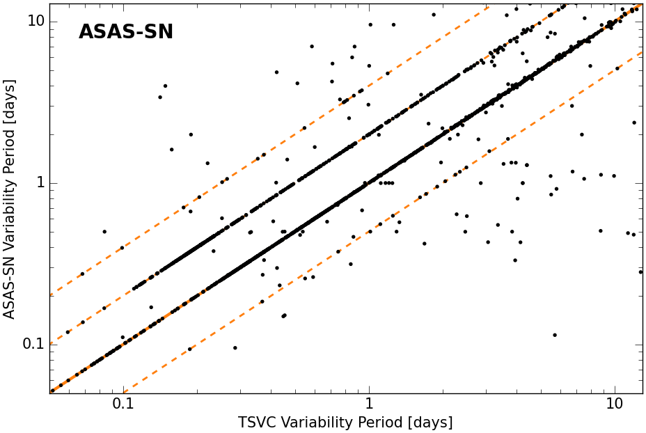
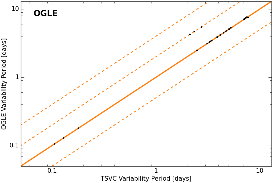
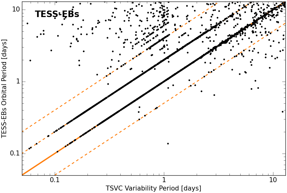
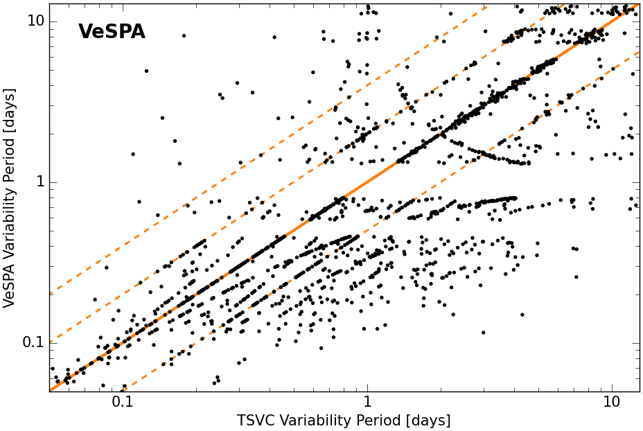
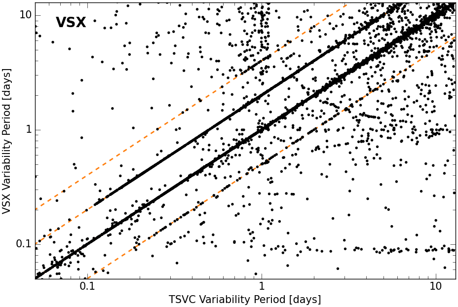
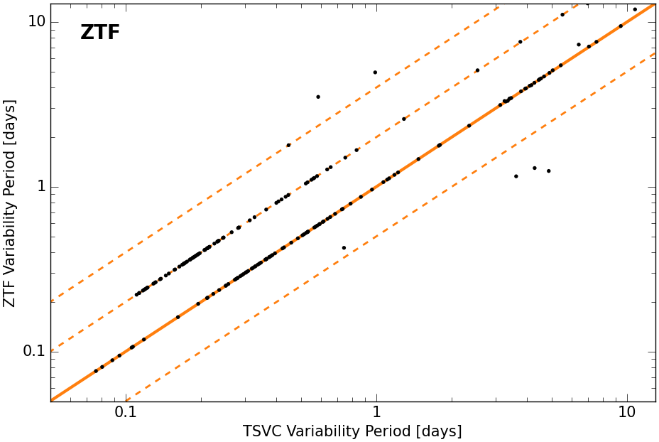
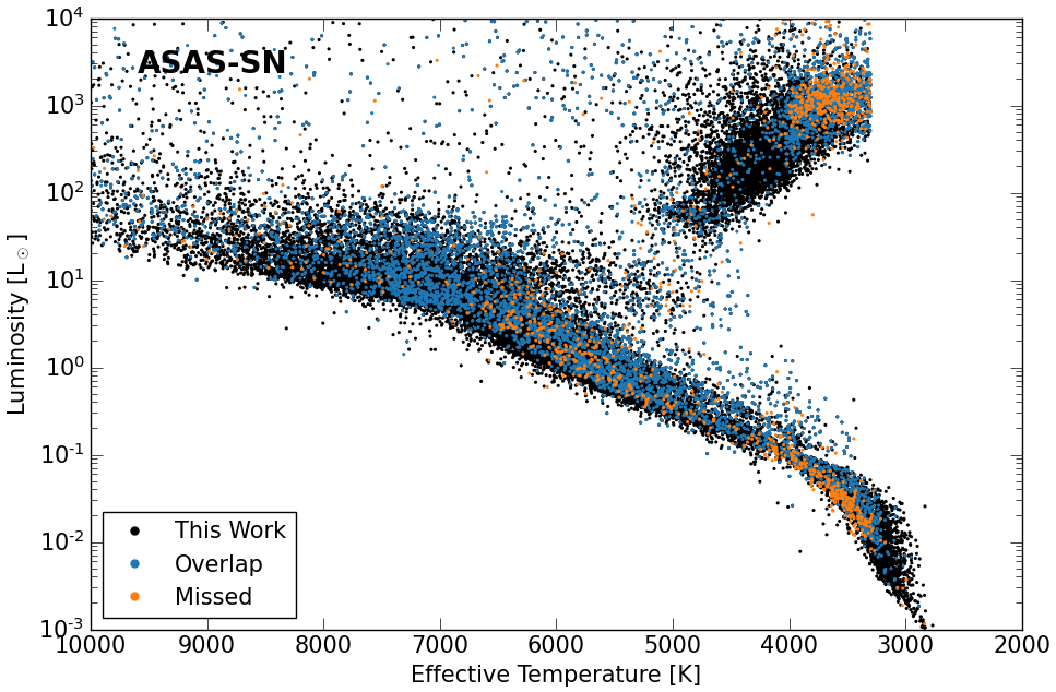
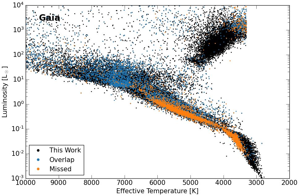
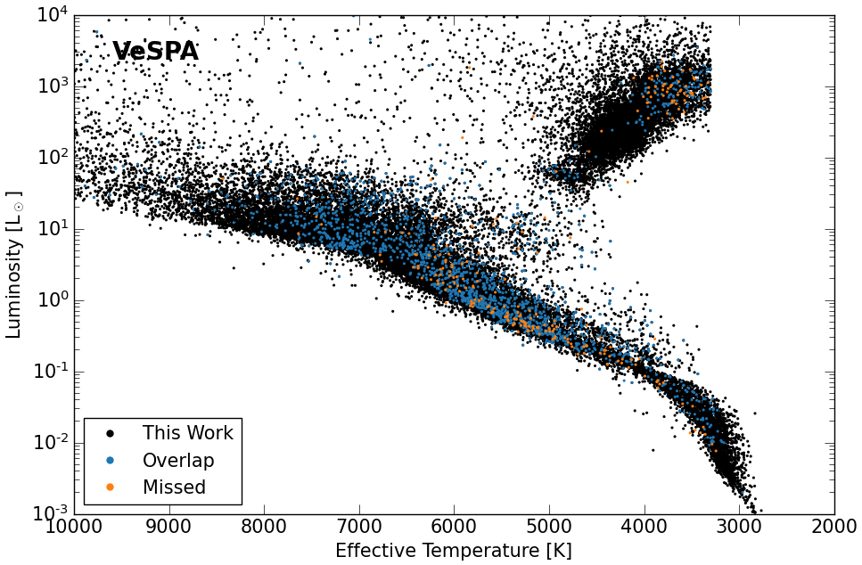
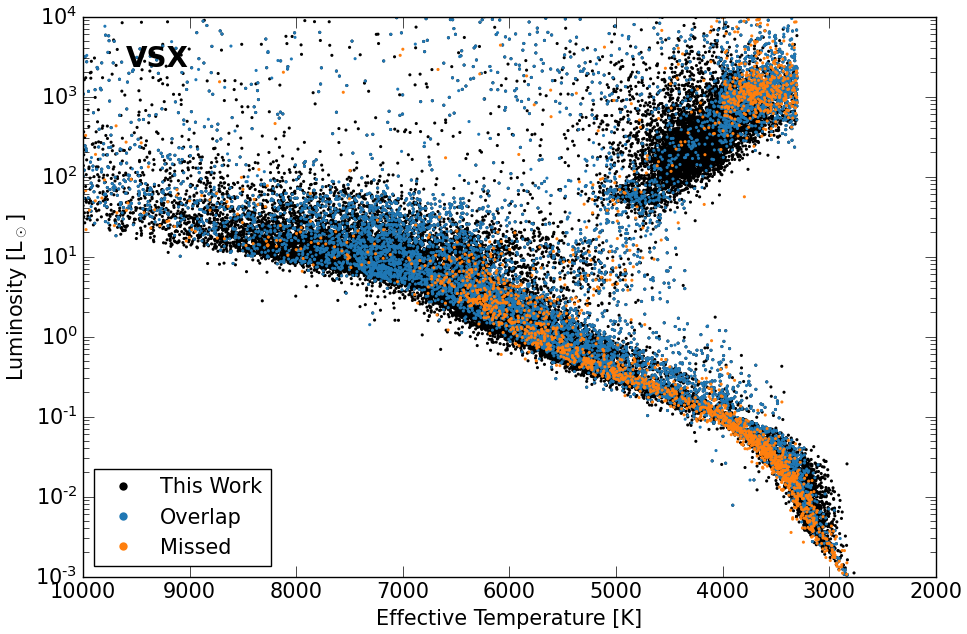
Here we compare the contents of variable stars in our catalog with those identified in several other ground- and space-based surveys. In particular, we select the following variability surveys and catalogs: SuperWASP: VeSPA (Pollacco et al., 2006; McMaster et al., 2021; Thiemann et al., 2021), OGLE (Udalski et al., 2008), ASAS-SN (Jayasinghe et al., 2018), Gaia DR3 (Gaia Collaboration et al., 2021; Eyer et al., 2022), ZTF (Yao et al., 2019; Chen et al., 2020), TESS-EBs (Prša et al. 2022; http://dx.doi.org/10.17909/t9-9gm4-fx30 (catalog DOI: 10.17909/t9-9gm4-fx30)), and the AAVSO International Variable Star Index (VSX). In order to evaluate our efforts at identifying variable stars, we only compare the stars from these surveys that overlap with our base sample of stars where we searched for periodicity in their 2-min light curves obtained during TESS Sectors 1–26. For the Gaia DR3, ASAS-SN, and TESS-EB catalogs we are able to match targets using their TIC or Gaia identifiers. Otherwise, we perform a 1″ search radius based on their RA and Dec. Table 4 shows the total number of stars that were successfully cross-identified from each survey compared to our base sample ($N_{\mathrm{tot}}$) and the number of stars that were also detected as variable in our catalog ($N_{\mathrm{var}}$). In total, there are 18,734 unique stars that overlap between this catalog and these existing catalogs, which implies that the catalog that we present in this work includes $\sim$65,000 new variable stars. We show how the measured variability periods compare between our variability catalog and each of the other surveys in Figure 15 (excluding Gaia DR3). In addition to highlighting matching variability periods (solid orange line), Figure 15 also highlights common harmonic aliases where our variability periods are different from those reported in other catalogs by factors of two or four (dashed orange lines). Harmonic aliases are especially often found for eclipsing binaries in cases where the shape and depth of the secondary eclipse closely matches that of the primary eclipse. Our variability search often identifies eclipsing binaries at half of their actual orbital period when the shape and depth of the secondary eclipse closely matches that of the primary eclipse. When comparing variability periods derived in this paper with eclipsing binary orbital periods reported by the TESS-EBs catalog (center left panel), we find that our analysis tends to select shorter-period harmonic aliases that can be many times shorter than the orbital period. Of note are some instances of eccentric eclipsing binaries that are identified as being variable at odd harmonic aliases (e.g., three or five times shorter). The identification of eclipsing binaries at certain eccentricities is a by-product of the LS periodogram assigning high LS power to the unequally spaced primary and secondary eclipses. The variability period comparisons with variability catalogs derived from ground-based observational surveys (i.e., VeSPA and VSX) in Figure 15 reveal arc-like features, which are caused by aliases between the true signal and the diurnal observing window (see Fig. 24 in VanderPlas, 2018). Besides these well-understood aliases, there is overall good agreement between the variability periods in our catalog and those reported by other stellar variability surveys. For the variability periods measured to be $<$13 days, 93%, 100%, 84%, 54%, 60%, and 97% of the variability periods reported in the ASAS-SN, OGLE, TESS-EBs, VeSPA, VSX, and ZTF catalogs, respectively, agree within 10% of our variability period measurement, or are within 10% of twice or half of our variability period measurement. However, the agreement between our variability period measurements and those reported in the ASAS-SN, OGLE, and ZTF catalogs is much better, with a median scatter that is less than 1%.

Table 4: Number of Targets Matched Between Stellar Variability Catalogs

Survey Name	$N_{\mathrm{tot}}$	$N_{\mathrm{var}}$
ASAS-SN	9830	8278
Gaia DR3	14309	10281
OGLE	35	33
TESS-EBs	3692	3365
VeSPA	2132	1872
VSX	13398	10741
ZTF	286	256

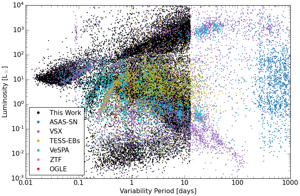
In Figure 16, we show how variable stars from ASAS-SN, Gaia DR3, VeSPA, and VSX are distributed across the HRD. The stars that are identified as significantly variable in both our catalog and the respective catalog are indicated by the blue points ($N_{\mathrm{var}}$ in Table 4). The stars listed as variables in the other catalog that are missed by our catalog are indicated by the orange points. Figure 17 shows the period-luminosity relationship for all variable stars identified in the selected catalogs (excluding Gaia DR3). It can be seen that many stars exhibit variability at periods longer than our 13-day search limit, primarily due to the longer observing baselines of ground-based observations available to ASAS-SN, VSX, and VeSPA. ASAS-SN especially excels at identifying variable stars with periodicities on timescales of several hundred days, and the VSX and VeSPA catalogs fill in the parameter space for periodic variability at 10–100 days. Most notably, the variable stars from the VSX and VeSPA catalogs further extend the linear trends observed between luminosity and variability period ($\sim$0.05–100 days), where higher luminosity giant stars and lower luminosity main sequence stars both tend to have longer variability periods (presumably their rotation periods) compared to lower luminosity giants and higher luminosity (i.e., hotter) main sequence stars. Stars with longer variability periods ($>$13 days) could largely account for the stars that did not make the cut into our variability catalog despite being included in our LS periodogram search (orange points in Figure 16). The TESS-EBs catalog largely identifies stars along the tight period-luminosity relationship for over-contact binary systems, but also identifies many detached binaries with orbital periods of 0.5–20 days that span luminosities of 1–100 L_⊙. The luminosities, in the case of binary systems, are still calculated using the reported effective temperature and stellar radius in the TICv8 catalog and assuming a single star, which results in binaries being offset from the main sequence towards higher luminosities in the HRD (e.g., Gaia Collaboration et al., 2018, 2019). The ZTF catalog primarily identifies over-contact binary systems, with a few rotational variables. There are very few stars that overlap with our sample from the OGLE survey, but the majority are high-luminosity giant stars. The Gaia DR3 variability periods are not included in Figure 17. However, based on the HRDs shown in Figure 16, it appears that Gaia DR3 variable stars cover a similar parameter space as the VSX catalog.

Compared to these other variability catalogs, our methodology and use of TESS photometry tends to identify new variable stars at the high- and low-temperature ends of the main sequence, and lower luminosity giant stars. The 2-min cadence continuous-stare strategy of TESS is especially ideal for identifying photometric variability on short timescales and at a higher precision than is possible for ground-based surveys, such that new variable stars with short periodicities ($\ll$1 day) or that are relatively faint (e.g., M-dwarfs) should not come as a surprise even when compared to extensive community-driven efforts such as VSX.

We recognize that this is not an exhaustive list of all surveys that observed these stars—especially given that TESS prioritized bright, nearby dwarf stars across nearly the entire sky suitable for the detection of small transiting exoplanets. However, we have demonstrated that there is sufficient overlap and consistent variability period measurements between our catalog and several other variability catalogs from the literature. Furthermore, our catalog includes many new variables that were likely beneath the photometric amplitude detection limit of ground-based surveys or periodic with a cadence that is aliased with ground-based observing strategies.

Figure 15: Comparison of the measured variability periods between our variability catalog and six other variable star surveys: ASAS-SN (top left), OGLE (top right), TESS-EBs (center left), VeSPA (center right), VSX (bottom left), and ZTF (bottom right). A perfect match between the variability periods is indicated by the solid orange line. The 2:1 and 4:1 alias periods are indicated by the dashed orange lines.

Figure 16: The locations of stars on the HR diagram for those matched between our analyzed sample and four other variable star surveys: ASAS-SN (top left), Gaia DR3 (top right), VeSPA (bottom left), and VSX (bottom right). All stars included in our variability catalog are shown by the black points. The stars that are variable in the respective survey and are also included in our variability catalog are indicated by the blue points. The stars that are identified as variable in the compared survey, but not identified in this work are highlighted by the orange points.

Figure 17: Same as Figure 8, but the colored points indicate that they are found in other variability catalogs.

4.4 Future Directions

The work presented in this paper is only an initial step in detecting and analyzing stellar variability using TESS data. There are numerous ways to expand upon this work. A natural next step that we are already working on is to extend the periodicity search beyond 13 days by stitching TESS observations across multiple sectors from the Simple Aperture Photometry, which will be especially powerful for examining stars in the TESS CVZs. Furthermore, there are now multiple pipelines extracting light curves of stars not selected for 2-min cadence observation, but are observed in the FFIs. These include light curves from QLP (Huang et al., 2020), TESS-SPOC (Caldwell et al., 2020), DIA (Oelkers et al., 2018), and DIAMANTE (Montalto et al., 2020), along with customized extraction tools for individual targets such as lightkurve (Lightkurve Collaboration et al., 2018), eleanor (Feinstein et al., 2019), and giants (Saunders et al., 2022). The availability of truly complete magnitude-limited stellar samples available from the FFIs would allow a future population analysis of variability unaffected by the target selection process for the 2-min cadence targets. For example, Kounkel et al. (2022) recently explored rotational variability that is detectable from the FFIs, which would be a valuable work for comparison when exploring the FFIs for broad variability.

An additional extension of this work is to combine the TESS light curves with photometry from other wide-field surveys. Ground-based surveys such as ASAS (Pojmanski, 2002), HATNet (Hartman et al., 2004), KELT (Oelkers et al., 2018), SuperWASP (Pollacco et al., 2006), ASAS-SN (Jayasinghe et al., 2018), and ZTF (Yao et al., 2019) cover large fractions of the sky with broadband photometry (typically in a single bandpass) over long periods of time. While the data from these surveys do not reach the photometric precision or duty cycle of TESS, they do cover much longer time frames. Combining TESS photometry with ground-based archival data will allow us to search for longer-term variations or changes in variability.

Lastly, there are a number of efforts underway to classify photometric variables with much finer physical and observational categories than has been done in this work. Notable examples are the OGLE project (Udalski et al., 2008), the Gaia DR3 variability search (Gaia Collaboration et al., 2021; Rimoldini et al., 2022), specific types of variable stars observed with TESS (e.g., Antoci et al., 2019; Howard et al., 2020b; Hon et al., 2021; Avallone et al., 2022; Barac et al., 2022; Holcomb et al., 2022; Prša et al., 2022; Kurtz, 2022; Saunders et al., 2022), and many others. The TESS Asteroseismic Science Operations Center (TASOC) is engaged in much more detailed and individualized analysis of certain types of stellar variability (Audenaert et al., 2021). Additionally, both supervised and unsupervised machine learning classification tools have been deployed to automatically classify variable stars (e.g., Blomme et al., 2010; Audenaert et al., 2021; Barbara et al., 2022; Claytor et al., 2022). We hope that the more limited variability characteristics and broad quantitative parameters we have presented here, along with the open description of our selection and threshold procedures, can be useful for such projects going forward.

5 Summary

We used TESS Prime Mission 2-min cadence photometry to search for stellar variability in $\sim$200,000 stars. Using a LS periodogram and ACF, we searched for photometric periodic variability on timescales up to 13 days in the light curves observed from each TESS sector. In Tables 1–3, we present our variability catalog, which includes $\sim$46,000 stars that are considered astrophysically variable to high confidence. In Section 4.1, we identify several trends of variability on the HRD and period–luminosity diagram. We find that the photometric variability period and amplitude of variability can be used as significant metrics for classifying different types of variability across the HRD. Furthermore, the distribution of stars in period–luminosity space reveals important information about different astrophysical mechanisms driving stellar variability. After careful consideration of variations caused by TESS spacecraft systematics, we also identify a dearth of dwarf star variability around 1.5–2 days (see Figure 11) where the astrophysical mechanism is not currently well-understood.

Overall, this work presents a broad overview of stellar variability observed across nearly the entire sky, but presents many opportunities for future investigations into stellar astrophysics and how stellar variability may affect exoplanetary systems. Stellar variability has already been shown to be a source for false positive exoplanet detections (e.g., Henry et al., 2002; Robertson et al., 2014; Robertson & Mahadevan, 2014; Robertson et al., 2015; Kane et al., 2016; Hojjatpanah et al., 2020; Niraula et al., 2022; Simpson et al., 2022), but avoiding active stars in exoplanet studies has also led to observational biases against planets around stars of certain spectral types and stages of evolution that tend to be particularly active (Simpson et al. 2023, submitted). Since all stars are variable at some point in their lifetime, understanding how stellar activity affects the measurements of exoplanet properties is a critical step towards understanding how star-planet systems—and especially planetary atmospheres—evolve over time.

The authors thank Guillermo Torres for helpful conversations and insight into the interpretations of this work. The authors acknowledge support from NASA grants 80NSSC18K0544 and 80NSSC18K0445, funded through the Exoplanet Research Program (XRP), and NASA grant 80NSSC20K0447 funded through the ADAP program. T.F. acknowledges support from the University of California President’s Postdoctoral Fellowship Program. This work was supported by a research grant (00028173) from VILLUM FONDEN. Funding for the Stellar Astrophysics Centre is provided by The Danish National Research Foundation (Grant agreement no.: DNRF106). D.H. acknowledges support from the Alfred P. Sloan Foundation and the National Aeronautics and Space Administration (80NSSC21K0652). We acknowledge the use of public TESS data from pipelines at the TESS Science Office and at the TESS Science Processing Operations Center. Resources supporting this work were provided by the NASA High-End Computing (HEC) Program through the NASA Advanced Supercomputing (NAS) Division at Ames Research Center for the production of the SPOC data products. All of the data presented in this paper were obtained from the Mikulski Archive for Space Telescopes (MAST). The specific observations analyzed can be accessed via http://dx.doi.org/10.17909/t9-nmc8-f686 (catalog DOI: 10.17909/t9-nmc8-f686). STScI is operated by the Association of Universities for Research in Astronomy, Inc., under NASA contract NAS5-26555. Support for MAST for non-HST data is provided by the NASA Office of Space Science via grant NNX13AC07G and by other grants and contracts. This paper includes data collected with the TESS mission, obtained from the MAST data archive at the Space Telescope Science Institute (STScI). Funding for the TESS mission is provided by the NASA Explorer Program. STScI is operated by the Association of Universities for Research in Astronomy, Inc., under NASA contract NAS 5–26555. This research made use of Lightkurve, a Python package for Kepler and TESS data analysis (Lightkurve Collaboration et al., 2018). We acknowledge with thanks the variable star observations from the AAVSO International Database contributed by observers worldwide and used in this research.

References

- Angus et al. (2019) Angus, R., Morton, T. D., Foreman-Mackey, D., et al. 2019, AJ, 158, 173, doi: 10.3847/1538-3881/ab3c53
- Antoci et al. (2019) Antoci, V., Cunha, M. S., Bowman, D. M., et al. 2019, MNRAS, 490, 4040, doi: 10.1093/mnras/stz2787
- Astropy Collaboration et al. (2013) Astropy Collaboration, Robitaille, T. P., Tollerud, E. J., et al. 2013, A&A, 558, A33, doi: 10.1051/0004-6361/201322068
- Astropy Collaboration et al. (2018) Astropy Collaboration, Price-Whelan, A. M., Sipőcz, B. M., et al. 2018, AJ, 156, 123, doi: 10.3847/1538-3881/aabc4f
- Astudillo-Defru et al. (2017) Astudillo-Defru, N., Delfosse, X., Bonfils, X., et al. 2017, A&A, 600, A13, doi: 10.1051/0004-6361/201527078
- Audenaert et al. (2021) Audenaert, J., Kuszlewicz, J. S., Handberg, R., et al. 2021, AJ, 162, 209, doi: 10.3847/1538-3881/ac166a
- Avallone et al. (2022) Avallone, E. A., Tayar, J. N., van Saders, J. L., et al. 2022, ApJ, 930, 7, doi: 10.3847/1538-4357/ac60a1
- Barac et al. (2022) Barac, N., Bedding, T. R., Murphy, S. J., & Hey, D. R. 2022, arXiv e-prints, arXiv:2207.00343. https://arxiv.org/abs/2207.00343
- Barbara et al. (2022) Barbara, N. H., Bedding, T. R., Fulcher, B. D., Murphy, S. J., & Van Reeth, T. 2022, MNRAS, doi: 10.1093/mnras/stac1515
- Basri et al. (2011) Basri, G., Walkowicz, L. M., Batalha, N., et al. 2011, AJ, 141, 20, doi: 10.1088/0004-6256/141/1/20
- Blomme et al. (2010) Blomme, J., Debosscher, J., De Ridder, J., et al. 2010, ApJ, 713, L204, doi: 10.1088/2041-8205/713/2/L204
- Böhm-Vitense (2007) Böhm-Vitense, E. 2007, ApJ, 657, 486, doi: 10.1086/510482
- Borucki et al. (2010) Borucki, W. J., Koch, D., Basri, G., et al. 2010, Science, 327, 977, doi: 10.1126/science.1185402
- Briegal et al. (2022) Briegal, J. T., Gillen, E., Queloz, D., et al. 2022, MNRAS, 513, 420, doi: 10.1093/mnras/stac898
- Caldwell et al. (2020) Caldwell, D. A., Tenenbaum, P., Twicken, J. D., et al. 2020, Research Notes of the American Astronomical Society, 4, 201, doi: 10.3847/2515-5172/abc9b3
- Chabrier & Baraffe (1997) Chabrier, G., & Baraffe, I. 1997, A&A, 327, 1039. https://arxiv.org/abs/astro-ph/9704118
- Chaplin & Miglio (2013) Chaplin, W. J., & Miglio, A. 2013, ARA&A, 51, 353, doi: 10.1146/annurev-astro-082812-140938
- Chen et al. (2020) Chen, X., Wang, S., Deng, L., et al. 2020, ApJS, 249, 18, doi: 10.3847/1538-4365/ab9cae
- Ciardi et al. (2015) Ciardi, D. R., Beichman, C. A., Horch, E. P., & Howell, S. B. 2015, ApJ, 805, 16, doi: 10.1088/0004-637X/805/1/16
- Ciardi et al. (2011) Ciardi, D. R., von Braun, K., Bryden, G., et al. 2011, AJ, 141, 108, doi: 10.1088/0004-6256/141/4/108
- Claytor et al. (2022) Claytor, Z. R., van Saders, J. L., Llama, J., et al. 2022, ApJ, 927, 219, doi: 10.3847/1538-4357/ac498f
- Dong et al. (2018) Dong, C., Jin, M., Lingam, M., et al. 2018, Proceedings of the National Academy of Science, 115, 260, doi: 10.1073/pnas.1708010115
- Dong et al. (2017) Dong, C., Lingam, M., Ma, Y., & Cohen, O. 2017, ApJ, 837, L26, doi: 10.3847/2041-8213/aa6438
- Eyer et al. (2022) Eyer, L., Audard, M., Holl, B., et al. 2022, arXiv e-prints, arXiv:2206.06416, doi: 10.48550/arXiv.2206.06416
- Feinstein et al. (2019) Feinstein, A. D., Montet, B. T., Foreman-Mackey, D., et al. 2019, PASP, 131, 094502, doi: 10.1088/1538-3873/ab291c
- Ferreira Lopes et al. (2015) Ferreira Lopes, C. E., Leão, I. C., de Freitas, D. B., et al. 2015, A&A, 583, A134, doi: 10.1051/0004-6361/201424900
- Fulton et al. (2017) Fulton, B. J., Petigura, E. A., Howard, A. W., et al. 2017, AJ, 154, 109, doi: 10.3847/1538-3881/aa80eb
- Gaia Collaboration et al. (2016) Gaia Collaboration, Prusti, T., de Bruijne, J. H. J., et al. 2016, A&A, 595, A1, doi: 10.1051/0004-6361/201629272
- Gaia Collaboration et al. (2018) Gaia Collaboration, Babusiaux, C., van Leeuwen, F., et al. 2018, A&A, 616, A10, doi: 10.1051/0004-6361/201832843
- Gaia Collaboration et al. (2019) Gaia Collaboration, Eyer, L., Rimoldini, L., et al. 2019, A&A, 623, A110, doi: 10.1051/0004-6361/201833304
- Gaia Collaboration et al. (2021) Gaia Collaboration, Brown, A. G. A., Vallenari, A., et al. 2021, A&A, 649, A1, doi: 10.1051/0004-6361/202039657
- Gaia Collaboration et al. (2022) Gaia Collaboration, Gaia Collaboration, De Ridder, J., et al. 2022, arXiv e-prints, arXiv:2206.06075. https://arxiv.org/abs/2206.06075
- Ginsburg et al. (2019) Ginsburg, A., Sipőcz, B. M., Brasseur, C. E., et al. 2019, AJ, 157, 98, doi: 10.3847/1538-3881/aafc33
- Gosnell et al. (2022) Gosnell, N. M., Gully-Santiago, M. A., Leiner, E. M., & Tofflemire, B. M. 2022, ApJ, 925, 5, doi: 10.3847/1538-4357/ac3668
- Guerrero et al. (2021) Guerrero, N. M., Seager, S., Huang, C. X., et al. 2021, ApJS, 254, 39, doi: 10.3847/1538-4365/abefe1
- Gunell et al. (2018) Gunell, H., Maggiolo, R., Nilsson, H., et al. 2018, A&A, 614, L3, doi: 10.1051/0004-6361/201832934
- Günther et al. (2020) Günther, M. N., Zhan, Z., Seager, S., et al. 2020, AJ, 159, 60, doi: 10.3847/1538-3881/ab5d3a
- Han et al. (2021) Han, H.-G., Cui, K.-M., Liu, J.-F., et al. 2021, Research in Astronomy and Astrophysics, 21, 142, doi: 10.1088/1674-4527/21/6/142
- Harris et al. (2020) Harris, C. R., Millman, K. J., van der Walt, S. J., et al. 2020, Nature, 585, 357, doi: 10.1038/s41586-020-2649-2
- Hartman et al. (2004) Hartman, J. D., Bakos, G., Stanek, K. Z., & Noyes, R. W. 2004, AJ, 128, 1761, doi: 10.1086/423920
- Heinze et al. (2018) Heinze, A. N., Tonry, J. L., Denneau, L., et al. 2018, AJ, 156, 241, doi: 10.3847/1538-3881/aae47f
- Hekker & Christensen-Dalsgaard (2017) Hekker, S., & Christensen-Dalsgaard, J. 2017, A&A Rev., 25, 1, doi: 10.1007/s00159-017-0101-x
- Henry et al. (2002) Henry, G. W., Donahue, R. A., & Baliunas, S. L. 2002, ApJ, 577, L111, doi: 10.1086/344291
- Hirsch et al. (2017) Hirsch, L. A., Ciardi, D. R., Howard, A. W., et al. 2017, AJ, 153, 117, doi: 10.3847/1538-3881/153/3/117
- Hojjatpanah et al. (2020) Hojjatpanah, S., Oshagh, M., Figueira, P., et al. 2020, A&A, 639, A35, doi: 10.1051/0004-6361/202038035
- Holcomb et al. (2022) Holcomb, R. J., Robertson, P., Hartigan, P., Oelkers, R. J., & Robinson, C. 2022, arXiv e-prints, arXiv:2206.10629. https://arxiv.org/abs/2206.10629
- Hon et al. (2021) Hon, M., Huber, D., Kuszlewicz, J. S., et al. 2021, ApJ, 919, 131, doi: 10.3847/1538-4357/ac14b1
- Howard et al. (2020a) Howard, W. S., Corbett, H., Law, N. M., et al. 2020a, ApJ, 902, 115, doi: 10.3847/1538-4357/abb5b4
- Howard et al. (2020b) —. 2020b, ApJ, 895, 140, doi: 10.3847/1538-4357/ab9081
- Huang et al. (2020) Huang, C. X., Vanderburg, A., Pál, A., et al. 2020, Research Notes of the American Astronomical Society, 4, 204, doi: 10.3847/2515-5172/abca2e
- Huber et al. (2011) Huber, D., Bedding, T. R., Stello, D., et al. 2011, ApJ, 743, 143, doi: 10.1088/0004-637X/743/2/143
- Hunter (2007) Hunter, J. D. 2007, Computing in Science and Engineering, 9, 90, doi: 10.1109/MCSE.2007.55
- Irwin & Bouvier (2009) Irwin, J., & Bouvier, J. 2009, in The Ages of Stars, ed. E. E. Mamajek, D. R. Soderblom, & R. F. G. Wyse, Vol. 258, 363–374, doi: 10.1017/S1743921309032025
- Jackman et al. (2019) Jackman, J. A. G., Wheatley, P. J., Pugh, C. E., et al. 2019, MNRAS, 482, 5553, doi: 10.1093/mnras/sty3036
- Jayasinghe et al. (2018) Jayasinghe, T., Kochanek, C. S., Stanek, K. Z., et al. 2018, MNRAS, 477, 3145, doi: 10.1093/mnras/sty838
- Jenkins et al. (2016) Jenkins, J. M., Twicken, J. D., McCauliff, S., et al. 2016, in Society of Photo-Optical Instrumentation Engineers (SPIE) Conference Series, Vol. 9913, Software and Cyberinfrastructure for Astronomy IV, ed. G. Chiozzi & J. C. Guzman, 99133E, doi: 10.1117/12.2233418
- Kane (2014) Kane, S. R. 2014, ApJ, 782, 111, doi: 10.1088/0004-637X/782/2/111
- Kane (2018) —. 2018, ApJ, 861, L21, doi: 10.3847/2041-8213/aad094
- Kane & Gelino (2012) Kane, S. R., & Gelino, D. M. 2012, MNRAS, 424, 779, doi: 10.1111/j.1365-2966.2012.21265.x
- Kane et al. (2020) Kane, S. R., Roettenbacher, R. M., Unterborn, C. T., Foley, B. J., & Hill, M. L. 2020, \psj, 1, 36, doi: 10.3847/PSJ/abaab5
- Kane et al. (2016) Kane, S. R., Thirumalachari, B., Henry, G. W., et al. 2016, ApJ, 820, L5, doi: 10.3847/2041-8205/820/1/L5
- King (1991) King, J. R. 1991, Information Bulletin on Variable Stars, 3562, 1
- Kochukhov (2021) Kochukhov, O. 2021, A&A Rev., 29, 1, doi: 10.1007/s00159-020-00130-3
- Kounkel et al. (2022) Kounkel, M., Stassun, K. G., Bouma, L. G., et al. 2022, arXiv e-prints, arXiv:2206.13545. https://arxiv.org/abs/2206.13545
- Kraft (1967) Kraft, R. P. 1967, ApJ, 150, 551, doi: 10.1086/149359
- Kreidberg et al. (2019) Kreidberg, L., Koll, D. D. B., Morley, C., et al. 2019, Nature, 573, 87, doi: 10.1038/s41586-019-1497-4
- Kurtz (2022) Kurtz, D. 2022, in Annual Conference and General Assembly of the African Astronomical Society, 1. https://arxiv.org/abs/2201.11629
- Lammer et al. (2003) Lammer, H., Selsis, F., Ribas, I., et al. 2003, ApJ, 598, L121, doi: 10.1086/380815
- Leiner et al. (2017) Leiner, E., Mathieu, R. D., & Geller, A. M. 2017, ApJ, 840, 67, doi: 10.3847/1538-4357/aa6aff
- Leiner et al. (2022) Leiner, E. M., Geller, A. M., Gully-Santiago, M. A., Gosnell, N. M., & Tofflemire, B. M. 2022, ApJ, 927, 222, doi: 10.3847/1538-4357/ac53b1
- Lightkurve Collaboration et al. (2018) Lightkurve Collaboration, Cardoso, J. V. d. M., Hedges, C., et al. 2018, Lightkurve: Kepler and TESS time series analysis in Python, Astrophysics Source Code Library. http://ascl.net/1812.013
- Lomb (1976) Lomb, N. R. 1976, Ap&SS, 39, 447, doi: 10.1007/BF00648343
- Mathieu et al. (2003) Mathieu, R. D., van den Berg, M., Torres, G., et al. 2003, AJ, 125, 246, doi: 10.1086/344944
- McMaster et al. (2021) McMaster, A., Norton, A. J., Dickinson, H. J., Thiemann, H. B., & Kolb, U. C. 2021, Research Notes of the American Astronomical Society, 5, 228, doi: 10.3847/2515-5172/ac2de8
- Meibom et al. (2009) Meibom, S., Mathieu, R. D., & Stassun, K. G. 2009, ApJ, 695, 679, doi: 10.1088/0004-637X/695/1/679
- Montalto et al. (2020) Montalto, M., Borsato, L., Granata, V., et al. 2020, MNRAS, 498, 1726, doi: 10.1093/mnras/staa2438
- Mosser et al. (2012) Mosser, B., Elsworth, Y., Hekker, S., et al. 2012, A&A, 537, A30, doi: 10.1051/0004-6361/201117352
- Murphy et al. (2019) Murphy, S. J., Hey, D., Van Reeth, T., & Bedding, T. R. 2019, MNRAS, 485, 2380, doi: 10.1093/mnras/stz590
- Murray-Clay et al. (2009) Murray-Clay, R. A., Chiang, E. I., & Murray, N. 2009, ApJ, 693, 23, doi: 10.1088/0004-637X/693/1/23
- Newton et al. (2017) Newton, E. R., Irwin, J., Charbonneau, D., et al. 2017, ApJ, 834, 85, doi: 10.3847/1538-4357/834/1/85
- Niraula et al. (2022) Niraula, P., Shporer, A., Wong, I., & de Wit, J. 2022, AJ, 163, 172, doi: 10.3847/1538-3881/ac4f64
- Oelkers et al. (2018) Oelkers, R. J., Rodriguez, J. E., Stassun, K. G., et al. 2018, AJ, 155, 39, doi: 10.3847/1538-3881/aa9bf4
- Owen & Wu (2013) Owen, J. E., & Wu, Y. 2013, ApJ, 775, 105, doi: 10.1088/0004-637X/775/2/105
- Owen & Wu (2017) —. 2017, ApJ, 847, 29, doi: 10.3847/1538-4357/aa890a
- Pojmanski (2002) Pojmanski, G. 2002, Acta Astron., 52, 397. https://arxiv.org/abs/astro-ph/0210283
- Pollacco et al. (2006) Pollacco, D. L., Skillen, I., Collier Cameron, A., et al. 2006, PASP, 118, 1407, doi: 10.1086/508556
- Prša et al. (2022) Prša, A., Kochoska, A., Conroy, K. E., et al. 2022, ApJS, 258, 16, doi: 10.3847/1538-4365/ac324a
- Ricker et al. (2014) Ricker, G. R., Winn, J. N., Vanderspek, R., et al. 2014, in Society of Photo-Optical Instrumentation Engineers (SPIE) Conference Series, Vol. 9143, Space Telescopes and Instrumentation 2014: Optical, Infrared, and Millimeter Wave, ed. J. Oschmann, Jacobus M., M. Clampin, G. G. Fazio, & H. A. MacEwen, 914320, doi: 10.1117/12.2063489
- Ricker et al. (2015) Ricker, G. R., Winn, J. N., Vanderspek, R., et al. 2015, Journal of Astronomical Telescopes, Instruments, and Systems, 1, 014003, doi: 10.1117/1.JATIS.1.1.014003
- Rimoldini et al. (2022) Rimoldini, L., Holl, B., Gavras, P., et al. 2022, arXiv e-prints, arXiv:2211.17238, doi: 10.48550/arXiv.2211.17238
- Robertson et al. (2015) Robertson, P., Endl, M., Henry, G. W., et al. 2015, ApJ, 801, 79, doi: 10.1088/0004-637X/801/2/79
- Robertson & Mahadevan (2014) Robertson, P., & Mahadevan, S. 2014, ApJ, 793, L24, doi: 10.1088/2041-8205/793/2/L24
- Robertson et al. (2014) Robertson, P., Mahadevan, S., Endl, M., & Roy, A. 2014, Science, 345, 440, doi: 10.1126/science.1253253
- Sakuraba et al. (2019) Sakuraba, H., Kurokawa, H., & Genda, H. 2019, Icarus, 317, 48, doi: 10.1016/j.icarus.2018.05.035
- Saunders et al. (2022) Saunders, N., Grunblatt, S. K., Huber, D., et al. 2022, AJ, 163, 53, doi: 10.3847/1538-3881/ac38a1
- Scargle (1982) Scargle, J. D. 1982, ApJ, 263, 835, doi: 10.1086/160554
- Seager et al. (2007) Seager, S., Kuchner, M., Hier-Majumder, C. A., & Militzer, B. 2007, ApJ, 669, 1279, doi: 10.1086/521346
- Segura et al. (2010) Segura, A., Walkowicz, L. M., Meadows, V., Kasting, J., & Hawley, S. 2010, Astrobiology, 10, 751, doi: 10.1089/ast.2009.0376
- Simpson et al. (2022) Simpson, E., Fetherolf, T., Kane, S. R., Pepper, J., & Li, Z. 2022, arXiv e-prints, arXiv:2203.06191. https://arxiv.org/abs/2203.06191
- Smith et al. (2012) Smith, J. C., Stumpe, M. C., Van Cleve, J. E., et al. 2012, PASP, 124, 1000, doi: 10.1086/667697
- Soderblom (2010) Soderblom, D. R. 2010, ARA&A, 48, 581, doi: 10.1146/annurev-astro-081309-130806
- Stassun et al. (2018) Stassun, K. G., Oelkers, R. J., Pepper, J., et al. 2018, AJ, 156, 102, doi: 10.3847/1538-3881/aad050
- Stassun et al. (2019) Stassun, K. G., Oelkers, R. J., Paegert, M., et al. 2019, AJ, 158, 138, doi: 10.3847/1538-3881/ab3467
- Stello et al. (2014) Stello, D., Compton, D. L., Bedding, T. R., et al. 2014, ApJ, 788, L10, doi: 10.1088/2041-8205/788/1/L10
- Stumpe et al. (2014) Stumpe, M. C., Smith, J. C., Catanzarite, J. H., et al. 2014, PASP, 126, 100, doi: 10.1086/674989
- Stumpe et al. (2012) Stumpe, M. C., Smith, J. C., Van Cleve, J. E., et al. 2012, PASP, 124, 985, doi: 10.1086/667698
- Tarter et al. (2007) Tarter, J. C., Backus, P. R., Mancinelli, R. L., et al. 2007, Astrobiology, 7, 30, doi: 10.1089/ast.2006.0124
- Thiemann et al. (2021) Thiemann, H. B., Norton, A. J., Dickinson, H. J., McMaster, A., & Kolb, U. C. 2021, MNRAS, 502, 1299, doi: 10.1093/mnras/stab140
- Udalski et al. (2008) Udalski, A., Szymanski, M. K., Soszynski, I., & Poleski, R. 2008, Acta Astron., 58, 69. https://arxiv.org/abs/0807.3884
- van Saders & Pinsonneault (2013) van Saders, J. L., & Pinsonneault, M. H. 2013, ApJ, 776, 67, doi: 10.1088/0004-637X/776/2/67
- VanderPlas (2018) VanderPlas, J. T. 2018, ApJS, 236, 16, doi: 10.3847/1538-4365/aab766
- Virtanen et al. (2020) Virtanen, P., Gommers, R., Oliphant, T. E., et al. 2020, Nature Methods, 17, 261, doi: 10.1038/s41592-019-0686-2
- Wright et al. (2011) Wright, N. J., Drake, J. J., Mamajek, E. E., & Henry, G. W. 2011, ApJ, 743, 48, doi: 10.1088/0004-637X/743/1/48
- Wright et al. (2018) Wright, N. J., Newton, E. R., Williams, P. K. G., Drake, J. J., & Yadav, R. K. 2018, MNRAS, 479, 2351, doi: 10.1093/mnras/sty1670
- Yao et al. (2019) Yao, Y., Miller, A. A., Kulkarni, S. R., et al. 2019, ApJ, 886, 152, doi: 10.3847/1538-4357/ab4cf5
- Yu et al. (2020) Yu, J., Bedding, T. R., Stello, D., et al. 2020, MNRAS, 493, 1388, doi: 10.1093/mnras/staa300
- Ziaali et al. (2019) Ziaali, E., Bedding, T. R., Murphy, S. J., Van Reeth, T., & Hey, D. R. 2019, MNRAS, 486, 4348, doi: 10.1093/mnras/stz1110