An efficient nonlinear multigrid solver for the simulation of rarefied gas cavity flow

Abstract

We study efficient simulation of steady state for rarefied gas flow, which is modeled by the Boltzmann equation with BGK-type collision term. A nonlinear multigrid solver is proposed to resolve the efficiency issue by the following approaches. The unified framework of numerical regularized moment method is first adopted to derive the high-quality discretization of the underlying problem. A fast sweeping iteration is introduced to solve the derived discrete problem more efficiently than the usual time-integration scheme on a single level grid. Taking it as the smoother, the nonlinear multigrid solver is then established to significantly improve the convergence rate. The OpenMP-based parallelization is applied in the implementation to further accelerate the computation. Numerical experiments for two lid-driven cavity flows and a bottom-heated cavity flow are carried out to investigate the performance of the resulting nonlinear multigrid solver. All results show the efficiency and robustness of the solver for both first- and second-order spatial discretization.

Key words. Boltzmann equation, moment method, multigrid, rarefied gas flow, steady state

1 Introduction

Rarefied gas dynamics is a classical discipline of fluid mechanics, which studies gas flows in the situation when the molecular mean free path, compared with the characteristic length of problems, can not be negligible. Over the past several decades, it has attracted more and more attention in the high-tech fields including astronautics and micro-electro-mechanical systems, due to the rapid development of aerospace and semiconductor industries, etc. To describe the rarefied gas flows correctly, the Boltzmann equation, rather than the traditional continuum models such as Euler equations and Navier-Stokes equations, should be taken into account. Clearly, numerical methods are necessary to solve the Boltzmann equation. In practice, for a variety of applications, the original quadratic collision term of the Boltzmann equation can be approximated by a simplified relaxation model, e.g., the Bhatnagar-Gross-Krook (BGK) model [1], to get a considerable reduction of computational effort without loss of accuracy. However, because of the intrinsic high dimensional nature, it still encounters a big challenge to develop an accurate and efficient solver for the simplified Boltzmann equation, especially for a great of important purposes [28, 35, 34] when the steady state of problems has to be under investigation.

This work is concerned with efficient simulation of steady state for rarefied gas flows modeled by the Boltzmann equation with BGK-type relaxation models. To this end, we are interested in the framework of numerical regularized moment method originated in [9] and then developed in [12, 10, 11, 6] for discretization of the underlying problem. As one of the most powerful methods, the moment method derives a system of continuous equations, which can be viewed not only as an extended hydrodynamic model but also a high-order velocity discretization of the Boltzmann equation. The numerical regularized moment method enhances this system with a slight modification so that some desired properties, such as global hyperbolicity [5] and convergence [14, 4], could be well guaranteed for the revised moment system up to arbitrary order. Moreover, in the framework of numerical regularized moment method, the full discretization would be obtained formally by using the finite volume method for spatial discretization without explicitly writing out the moment system. Such a unified framework makes the practical application of high-order moment system much easier. Additionally, both first- and second-order spatial discretization are of interest in the present paper.

To efficiently solve the derived discrete steady-state problem, a fast sweeping iteration, based on the forward Euler scheme and the cell-by-cell Gauss-Seidel iteration with four alternating direction sweepings in two-dimensional (2D) case, is first proposed on a single level grid. In comparison to the forward Euler scheme, the present fast sweeping iteration would converge much faster, while takes for each iteration almost the same computational cost as four steps of the forward Euler scheme. It turns out that the fast sweeping iteration is usually more efficient than the forward Euler scheme. Indeed, it can also be observed that the fast sweeping iteration is more robust than the forward Euler scheme especially when the second-order spatial discretization is under consideration.

In view of that the multigrid method [3, 18] is one of the most popular acceleration techniques for steady-state computation, we then concentrate on the multigrid acceleration for our discrete problem. Actually, a nonlinear multigrid (NMG) iteration, which takes an SGS-Newton iteration as the smoother, has been successfully developed for the hyperbolic moment models in one-dimensional case [23]. In the current work, we generalize this NMG iteration to 2D case by using the previous fast sweeping iteration instead of the SGS-Newton iteration, and providing an appropriate construction of 2D restriction and prolongation operators. The resulting NMG solver would always converge within dozens of iterations, leading to a significant improvement in efficiency in comparison to the fast sweeping iteration. To further accelerate the computation, the OpenMP-based parallelization [15] is employed in the implementation of the NMG solver. Almost all operations, including for loop to traverse grid cells of a given grid, e.g., smoothing, restriction and prolongation, can be parallelized trivially without appreciably affecting the results, although it should be pointed out that the parallel fast sweeping iteration is not exactly equivalent to the serial fast sweeping iteration.

Finally, a number of numerical experiments for 2D cavity flows such as two lid-driven flows and a bottom-heated flow are presented to explore the behavior of the resulting NMG solver. The efficiency and robustness of it are well validated by numerical results for both first- and second-order spatial discretization.

The rest of this paper is organized as follows. In section 2, a brief review of the Boltzmann equation and the full discretization as well as the basic time-integration scheme are introduced. The details of three acceleration methods, namely, fast sweeping iteration, nonlinear multigrid method, and OpenMP-based parallelization, are described in section 3 to establish the final steady-state solver. Numerical experiments are presented in section 4, and a brief summary is given in the last section.

2 Model equations and basic numerical method

In this section, we will give a brief review of the governing model equations for rarefied gas dynamics, and introduce a unified framework of numerical method on a given single level grid by using the numerical regularized moment method.

2.1 Boltzmann equation with BGK-type collision term

Let $f(t,\boldsymbol{x},\boldsymbol{\xi})$ be the distribution function such that $f(t,\boldsymbol{x},\boldsymbol{\xi})\,\mathrm{d}\boldsymbol{x}\,\mathrm{d}\boldsymbol{\xi}$ gives the number of particles that locate in the infinitesimal cell $\,\mathrm{d}\boldsymbol{x}$ about $\boldsymbol{x}$ with velocities within the infinitesimal cell $\,\mathrm{d}\boldsymbol{\xi}$ about $\boldsymbol{\xi}$ at time $t$. For the rarefied gas in a 2D cavity, the evolution of $f$ can be well described by the Boltzmann equation

$$\dfrac{\partial{f}}{\partial{t}}+\boldsymbol{\xi}\cdot\nabla_{\boldsymbol{x}}f=Q[f,f],\quad t\in\mathbb{R}^{+},\quad\boldsymbol{x}\in\Omega\subset\mathbb{R}^{2},\quad\boldsymbol{\xi}\in\mathbb{R}^{3},$$ (1)

subject to some appropriate boundary conditions and the assumption $\frac{\partial f}{\partial x_{3}}\equiv 0$. Here the right-hand side $Q[f,f]$ is the collision term representing the interaction between gas molecules. It usually takes the quadratic form

$$Q[f,f](t,\boldsymbol{x},\boldsymbol{\xi})=\int_{\mathbb{R}^{3}}\int_{\mathbb{S}_{+}^{2}}B(|\boldsymbol{\xi}-\boldsymbol{\xi}_{*}|,\boldsymbol{n})(f^{\prime}f_{*}^{\prime}-ff_{*})\,\mathrm{d}\boldsymbol{n}\,\mathrm{d}\boldsymbol{\xi}_{*},$$ (2)

where the collision kernel $B(\cdot,\cdot)$ is a non-negative function determined by the potential between gas molecules, $\boldsymbol{n}\in\mathbb{S}_{+}^{2}$ is a unit vector directed along the line joining the centers of two colliding particles with pre-collision velocities $\boldsymbol{\xi}$ and $\boldsymbol{\xi}_{*}$, and $f_{*}=f(t,\boldsymbol{x},\boldsymbol{\xi}_{*})$, $f^{\prime}=f(t,\boldsymbol{x},\boldsymbol{\xi}^{\prime})$, $f_{*}^{\prime}=f(t,\boldsymbol{x},\boldsymbol{\xi}_{*}^{\prime})$, in which $\boldsymbol{\xi}^{\prime}$ and $\boldsymbol{\xi}_{*}^{\prime}$, given by

$$\boldsymbol{\xi}^{\prime}=\boldsymbol{\xi}-[(\boldsymbol{\xi}-\boldsymbol{\xi}_{*})\cdot\boldsymbol{n}]\boldsymbol{n},\quad\boldsymbol{\xi}_{*}^{\prime}=\boldsymbol{\xi}_{*}-[(\boldsymbol{\xi}_{*}-\boldsymbol{\xi})\cdot\boldsymbol{n}]\boldsymbol{n},$$

are the corresponding post-collision velocities of the two colliding particles.

While the distribution function $f$ gives a detailed information of the state of the gas, in most practical applications, we are mainly concerned about the macroscopic physical quantities, such as the mass density $\rho$, mean velocity $\boldsymbol{u}$, and temperature $\theta$, rather than the distribution function itself. For these quantities of interest, they are related to the moments of the distribution function as follows

$$\begin{aligned} &\rho(t,\boldsymbol{x})=m_{*}\int_{\mathbb{R}^{3}}f(t,\boldsymbol{x},\boldsymbol{\xi})\,\mathrm{d}\boldsymbol{\xi},\\ &\rho(t,\boldsymbol{x})\boldsymbol{u}(t,\boldsymbol{x})=m_{*}\int_{\mathbb{R}^{3}}\boldsymbol{\xi}f(t,\boldsymbol{x},\boldsymbol{\xi})\,\mathrm{d}\boldsymbol{\xi},\\ &\rho(t,\boldsymbol{x})|\boldsymbol{u}(t,\boldsymbol{x})|^{2}+3\rho(t,\boldsymbol{x})\theta(t,\boldsymbol{x})=m_{*}\int_{\mathbb{R}^{3}}|\boldsymbol{\xi}|^{2}f(t,\boldsymbol{x},\boldsymbol{\xi})\,\mathrm{d}\boldsymbol{\xi},\end{aligned}$$ (3)

where $m_{*}$ is the mass of a single gas molecule. Similarly, the stress tensor $\sigma_{ij}$, $i,j=1,2,3$, and the heat flux $\boldsymbol{q}$ are defined by

$$\begin{aligned} &\sigma_{ij}(t,\boldsymbol{x})=m_{*}\int_{\mathbb{R}^{3}}(\xi_{i}-u_{i}(t,\boldsymbol{x}))(\xi_{j}-u_{j}(t,\boldsymbol{x}))f(t,\boldsymbol{x},\boldsymbol{\xi})\,\mathrm{d}\boldsymbol{\xi}-\rho(t,\boldsymbol{x})\theta(t,\boldsymbol{x})\delta_{ij},\\ &\boldsymbol{q}(t,\boldsymbol{x})=\frac{m_{*}}{2}\int_{\mathbb{R}^{3}}|\boldsymbol{\xi}-\boldsymbol{u}(t,\boldsymbol{x})|^{2}(\boldsymbol{\xi}-\boldsymbol{u}(t,\boldsymbol{x}))f(t,\boldsymbol{x},\boldsymbol{\xi})\,\mathrm{d}\boldsymbol{\xi},\end{aligned}$$ (4)

where $\delta_{ij}$ is the Kronecker delta symbol.

It is obvious that the quadratic collision term 2 is the most complicated part in the Boltzmann equation, which leads to a great challenge for efficient numerical simulation. In recent years, some fast numerical methods have been successfully proposed to partially resolve the efficiency issue in the computation of 2, see e.g., [32, 16] for Fourier spectral method, [31] for Hermite spectral method and [8] for Burnett spectral method. However, lots of researchers are still very interested in the approach to approximate the quadratic collision term 2 by a simpler collision model, which is able to predict the major physical features of interest with a much smaller computational cost, in a number of situations at moderate Knudsen numbers. The most famous class of simplified collision models are the BGK-type relaxation models, which have the general form of

$$Q[f,f]\approx Q(f)=\nu(f^{\text{E}}-f),$$ (5)

where $\nu$ is the average collision frequency assumed independent of the molecular velocity, and $f^{\text{E}}$ is the local equilibrium distribution function depending on the specific model selected. In particular, we have

• For the simplest BGK model [1], $f^{\text{E}}$ is the local Maxwellian given by

  $$f^{\text{E}}(t,\boldsymbol{x},\boldsymbol{\xi})=\mathcal{M}_{f}(t,\boldsymbol{x},\boldsymbol{\xi})=\frac{\rho(t,\boldsymbol{x})}{m_{*}[2\pi\theta(t,\boldsymbol{x})]^{3/2}}\exp\left(-\frac{|\boldsymbol{\xi}-\boldsymbol{u}(t,\boldsymbol{x})|^{2}}{2\theta(t,\boldsymbol{x})}\right).$$ (6)

• For the ellipsoidal statistical BGK (ES-BGK) model [19], $f^{\text{E}}$ is an anisotropic Gaussian distribution defined by

  $$f^{\text{E}}(t,\boldsymbol{x},\boldsymbol{\xi})=\frac{\rho(t,\boldsymbol{x})}{m_{*}\sqrt{\det[2\pi{\boldsymbol{\Lambda}}]}}\exp\left(-\frac{1}{2}(\boldsymbol{\xi}-\boldsymbol{u}(t,\boldsymbol{x}))^{T}{\boldsymbol{\Lambda}}^{-1}(\boldsymbol{\xi}-\boldsymbol{u}(t,\boldsymbol{x}))\right),$$ (7)

  where ${\boldsymbol{\Lambda}}=(\lambda_{ij})$ is a $3\times 3$ matrix given by

  $$\lambda_{ij}(t,\boldsymbol{x})=\theta(t,\boldsymbol{x})\delta_{ij}+\left(1-\frac{1}{\Pr}\right)\frac{\sigma_{ij}(t,\boldsymbol{x})}{\rho(t,\boldsymbol{x})},\quad i,j=1,2,3,$$

  in which $\Pr$ is the Prandtl number.

• For the Shakhov model [30], $f^{\text{E}}$ is the product of the local Maxwellian and a cubic polynomial of $\boldsymbol{\xi}$ as

  $$f^{\text{E}}(t,\boldsymbol{x},\boldsymbol{\xi})=\left[1+\frac{(1-\Pr)(\boldsymbol{\xi}-\boldsymbol{u}(t,\boldsymbol{x}))\cdot\boldsymbol{q}(t,\boldsymbol{x})}{5\rho(t,\boldsymbol{x})[\theta(t,\boldsymbol{x})]^{2}}\left(\frac{|\boldsymbol{\xi}-\boldsymbol{u}(t,\boldsymbol{x})|^{2}}{\theta(t,\boldsymbol{x})}-5\right)\right]\mathcal{M}_{f}(t,\boldsymbol{x},\boldsymbol{\xi}).$$ (8)

It is apparent from 3 and 4 that $f^{\text{E}}$ is nonlinearly dependent on $f$ via the macroscopic physical quantities. In addition, both the ES-BGK model and the Shakhov model reduce to the BGK model in the case when $\Pr=1$.

In view of the enormous computational cost of the quadratic collision term 2, we shall mainly use the BGK-type relaxation models as examples in this work, to illustrate the framework of the present numerical method and to reveal the main features of the resulting solver.

2.2 Velocity discretization and moment system

In order to discretize the Boltzmann equation 1 in velocity space, we would like to use the Hermite spectral method, which first expands the distribution function into a series of Hermite functions as

$$f(t,\boldsymbol{x},\boldsymbol{\xi})=\sum_{\alpha\in\mathbb{N}^{3}}f_{\alpha}(t,\boldsymbol{x})\mathcal{H}_{\alpha}^{[\boldsymbol{\varpi},\vartheta]}(\boldsymbol{\xi}),$$ (9)

where $\mathcal{H}_{\alpha}^{[\boldsymbol{\varpi},\vartheta]}(\cdot)$ is the $\alpha$th basis function defined by

$$\mathcal{H}_{\alpha}^{[\boldsymbol{\varpi},\vartheta]}(\boldsymbol{\xi})=\frac{1}{m_{*}(2\pi\vartheta)^{3/2}\vartheta^{|\alpha|/2}}\prod\limits_{d=1}^{3}\mathit{He}_{\alpha_{d}}({v}_{d})\exp\left(-\frac{{v}_{d}^{2}}{2}\right),\quad{\boldsymbol{v}}=\frac{\boldsymbol{\xi}-\boldsymbol{\varpi}}{\sqrt{\vartheta}},~{}~{}\forall\boldsymbol{\xi}\in\mathbb{R}^{3},$$

and $f_{\alpha}(t,\boldsymbol{x})$ is the corresponding coefficient that is independent of $\boldsymbol{\xi}$. In the above expression, $|\alpha|$ is the sum of all components of the multi-dimensional index $\alpha$, i.e., $|\alpha|=\alpha_{1}+\alpha_{2}+\alpha_{3}$, and $\mathit{He}_{n}(\cdot)$ is the Hermite polynomial of degree $n$ given by

$$\mathit{He}_{n}(x)=(-1)^{n}\exp\left(\frac{x^{2}}{2}\right)\frac{\,\mathrm{d}^{n}}{\,\mathrm{d}x^{n}}\exp\left(-\frac{x^{2}}{2}\right).$$

The parameters $\boldsymbol{\varpi}\in\mathbb{R}^{3}$ and $\vartheta\in\mathbb{R}^{+}$ in the basis function could be either constants or variables depending on $t$ and $\boldsymbol{x}$. Besides to set them as constants for the most common Hermite spectral method, a popular approach, originated by Grad [17], is to adaptively choose $\boldsymbol{\varpi}$ and $\vartheta$ as the local mean velocity $\boldsymbol{u}$ and temperature $\theta$, respectively, according to the distribution function $f$ itself via 3. For the Grad method, we can easily deduce from 3 and 4 that

$$\begin{aligned} &f_{0}=\rho,\qquad f_{e_{1}}=f_{e_{2}}=f_{e_{3}}=0,\qquad\sum_{d=1}^{3}f_{2e_{d}}=0,\\ &\sigma_{ij}=(1+\delta_{ij})f_{e_{i}+e_{j}},\quad q_{i}=2f_{3e_{i}}+\sum_{d=1}^{3}f_{2e_{d}+e_{i}},\qquad i,j=1,2,3,\end{aligned}$$ (10)

where $e_{1}$, $e_{2}$, and $e_{3}$ denote the multi-dimensional indices $(1,0,0)$, $(0,1,0)$, and $(0,0,1)$, respectively. Moreover, it can be expected that the series 9 converges fast when the distribution function is smooth and not too far away from the Maxwellian. Actually, the first term of the series 9 already gives the local Maxwellian associated with the distribution function $f$. For the general choice of $\boldsymbol{\varpi}$ and $\vartheta$, the macroscopic physical quantities of interest can also be related directly to these two parameters and the low-order coefficients, i.e., $f_{\alpha}$ with $|\alpha|\leq 3$. We refer to [21] for the detailed relations in this general case. Additionally, as pointed out in [20], the convergence of the series 9 could usually be expected for a smooth distribution function if $\theta<2\vartheta$.

Due to the importance of the Grad method, we will restrict ourselves to the case of $\boldsymbol{\varpi}=\boldsymbol{u}$ and $\vartheta=\theta$ for the approximation of every distribution function in this paper. Numerically, the distribution function is approximated by a truncated series of order $M$, that is,

$$f(t,\boldsymbol{x},\boldsymbol{\xi})\approx\sum_{|\alpha|\leq M}f_{\alpha}(t,\boldsymbol{x})\mathcal{H}_{\alpha}^{[\boldsymbol{u}(t,\boldsymbol{x}),\theta(t,\boldsymbol{x})]}(\boldsymbol{\xi})\in\mathcal{F}_{M}^{[\boldsymbol{u},\theta]},$$ (11)

where $\mathcal{F}_{M}^{[\boldsymbol{u},\theta]}$ is the finite-dimensional linear space spanned by $\mathcal{H}_{\alpha}^{[\boldsymbol{u},\theta]}(\boldsymbol{\xi})$ for all $\alpha$ with $|\alpha|\leq M$. In view of the relation 10, we have that the unknown variables in the above approximation are $\boldsymbol{u}$, $\theta$, and all coefficients $f_{\alpha}$ with $|\alpha|\leq M$ except the coefficients with $|\alpha|=1$ and one of the coefficients with $|\alpha|=2$. Let $\boldsymbol{\varrho}$ represent the vector composed of these unknown quantities. Following the framework of deriving the regularized moment model from the Boltzmann equation 1 that was proposed in [5, 6], we can get a globally hyperbolic system for $\boldsymbol{\varrho}$, which can be written in a quasi-linear form as

$$\dfrac{\partial{\boldsymbol{\varrho}}}{\partial{t}}+{\bf{A}}_{1}(\boldsymbol{\varrho})\dfrac{\partial{\boldsymbol{\varrho}}}{\partial{x_{1}}}+{\bf{A}}_{2}(\boldsymbol{\varrho})\dfrac{\partial{\boldsymbol{\varrho}}}{\partial{x_{2}}}=\boldsymbol{S}(\boldsymbol{\varrho}),$$ (12)

where the left-hand side is derived from the left-hand side of the Boltzmann equation, and the right-hand side corresponds to the collision term. The detailed expression of the above system can be found for the Boltzmann equation with the ES-BGK model in [11] and with the Shakhov model in [10]. Here, we omit it since it has no effect on the description of the solver presented in this work.

Nevertheless, it is worth mentioning that the moment system 12 of order $M$ with $M\geq 2$ contains the classical hydrodynamic equations. In particular, the equations with the multi-dimensional indices $\alpha=0$ and $\alpha=e_{i}$, $i=1,2,3$, are the conservation laws for mass and momentum respectively. Therefore, the moment system of order $M$ is also known as the extended hydrodynamic equations in the literature.

2.3 Spatial finite volume discretization

It is tedious to discretize the moment system in spatial domain directly based on the form 12 for $\boldsymbol{\varrho}$. Alternatively, in the framework of the numerical regularized moment method originated in [9], the spatial discretization of 12 is designed in a unified approach for the moment system of arbitrary order, based on the underlying Boltzmann equation 1 with the truncated approximation 11. Our discretization given below is obtained following this approach.

In the rest of the paper, the spatial coordinates $x_{1}$ and $x_{2}$ as well as the associated notations will be replaced by $x$ and $y$, respectively, for convenience. Let the spatial domain $\Omega$ be simply a rectangle with the length of $L_{x}$ and the height of $L_{y}$. Suppose $\Omega$ is divided into a rectangular grid with $N_{x}\times N_{y}$ cells, for which the grid points are given by $(x_{i+1/2},y_{j+1/2})$, $i=0,1,\ldots,N_{x}$, $j=0,1,\ldots,N_{y}$. Let $f_{ij}(t,\boldsymbol{\xi})$ represent the average distribution function over the $(i,j)$th grid cell $[x_{i-1/2},x_{i+1/2}]\times[y_{j-1/2},y_{j+1/2}]$, $i=1,2,\ldots,N_{x}$, $j=1,2,\ldots,N_{y}$. Then by applying the finite volume method to the Boltzmann equation 1, we can obtain an ODE for the evolution of the average distribution function over each grid cell as

$$\dfrac{\,\mathrm{d}{f_{ij}}}{\,\mathrm{d}{t}}=-\left[\frac{F_{i+\frac{1}{2},j}-F_{i-\frac{1}{2},j}}{\Delta x_{i}}+\frac{F_{i,j+\frac{1}{2}}-F_{i,j-\frac{1}{2}}}{\Delta y_{j}}\right]+Q(f_{ij})=:\mathcal{R}_{ij}(\boldsymbol{f}),$$ (13)

where $\Delta x_{i}=x_{i+1/2}-x_{i-1/2}$ and $\Delta y_{j}=y_{j+1/2}-y_{j-1/2}$ are the length and height, respectively, of the $(i,j)$th cell, $Q(f_{ij})$ is the average of collision term over the $(i,j)$th cell, $\boldsymbol{f}$ is the vector composed of all $f_{ij}$, and $F_{i+1/2,j}$ represents the numerical flux defined at the boundary between the $(i,j)$th and $(i+1,j)$th cells. Other numerical fluxes are defined similarly, so they are omitted below.

With the assumption that all $f_{ij}(t,\boldsymbol{\xi})\in\mathcal{F}_{M}^{[\boldsymbol{u}_{ij},\theta_{ij}]}$, where $\boldsymbol{u}_{ij}(t)$ and $\theta_{ij}(t)$ are the averages of mean velocity and temperature, respectively, on the $(i,j)$th cell and the relation 10 holds for the expansion coefficients $f_{ij,\alpha}(t)$, let us investigate the approximation of 13 over the $(i,j)$th cell in $\mathcal{F}_{M}^{[\boldsymbol{u}_{ij},\theta_{ij}]}$. To this end, the four numerical fluxes and $Q(f_{ij})$ are first projected into $\mathcal{F}_{M}^{[\boldsymbol{u}_{ij},\theta_{ij}]}$, so that, for examples, we have formally that

$$\begin{aligned} &F_{i+\frac{1}{2},j}\approx\sum_{|\alpha|\leq M}F_{\alpha}(f_{i+\frac{1}{2},j}^{-},f_{i+\frac{1}{2},j}^{+})\mathcal{H}_{\alpha}^{[\boldsymbol{u}_{ij},\theta_{ij}]}(\boldsymbol{\xi}),\\ &Q(f_{ij})\approx\sum_{|\alpha|\leq M}Q_{ij,\alpha}\mathcal{H}_{\alpha}^{[\boldsymbol{u}_{ij},\theta_{ij}]}(\boldsymbol{\xi}),\end{aligned}$$ (14)

where the coefficients $F_{\alpha}$ depend on the left and right limits of distribution function, i.e., $f_{i+1/2,j}^{\pm}\in\mathcal{F}_{M}^{[\boldsymbol{u}_{i+1/2,j}^{\pm},\theta_{i+1/2,j}^{\pm}]}$, at the right boundary of the $(i,j)$th cell, and the coefficients $Q_{ij,\alpha}$ depend only on the $(i,j)$th distribution function $f_{ij}$. If the numerical flux is designed specially to reflect the hyperbolicity of the moment system 12, then after matching the coefficients in both sides of 13 for the same basis function $\mathcal{H}_{\alpha}^{[\boldsymbol{u}_{ij},\theta_{ij}]}(\boldsymbol{\xi})$, we will get a system which can equivalently be viewed as a spatial discretization of the moment system 12 on the $(i,j)$th cell.

In our numerical experiments, the numerical flux introduced in [11] is adopted. The detailed expression will not be given here for brevity. However, it is noted that in order to calculate the approximation of the numerical flux in $\mathcal{F}_{M}^{[\boldsymbol{u}_{ij},\theta_{ij}]}$ as 14, a transformation to project a function from one space $\mathcal{F}_{M}^{[\boldsymbol{\varpi},\vartheta]}$ into another space $\mathcal{F}_{M}^{[\tilde{\boldsymbol{\varpi}},\tilde{\vartheta}]}$ would be heavily involved, since the expansion of the distribution function $f_{ij}$ on each cell usually uses the basis functions with different parameters, and so are the expansions of $f_{i+1/2,j}^{\pm}$. Such a transformation is in fact one of cores of the unified discretization for the moment system of arbitrary order. A fast algorithm with the time complexity of $\mathcal{O}(M^{3})$ for it has been implemented in [9, 7]. For other parts of the present solver, this transformation will also be employed frequently, and may not be explicitly pointed out.

It remains to determine the distribution functions $f_{i+1/2,j}^{\pm}$ at all cell boundaries. Obviously, it is equivalent to directly determine the parameters $\boldsymbol{u}_{i+1/2,j}^{\pm}$, $\theta_{i+1/2,j}^{\pm}$, and all expansion coefficients $f_{i+1/2,j,\alpha}^{\pm}$ with $|\alpha|\leq M$. Taking the distribution functions on the left and right boundaries of the $(i,j)$th cell, i.e., $f_{i-1/2,j}^{+}$ and $f_{i+1/2,j}^{-}$, respectively, as examples, let us consider the reconstruction of them providing that the average distribution functions $f_{\iota j}\in\mathcal{F}_{M}^{[\boldsymbol{u}_{\iota j},\theta_{\iota j}]}$ on the $(\iota,j)$th cell, $\iota=i,i\pm 1$, are given. Using the same strategy as in [22], the corresponding parameters and expansion coefficients of $f_{i-1/2,j}^{+}$ and $f_{i+1/2,j}^{-}$ could be computed efficiently by avoiding the transformation mentioned above. To be specific, we have

$$\begin{aligned} \boldsymbol{u}_{i-1/2,j}^{+}=\boldsymbol{u}_{ij}-\frac{\Delta x_{i}}{2}\boldsymbol{g}_{ij},&\qquad\boldsymbol{u}_{i+1/2,j}^{-}=\boldsymbol{u}_{ij}+\frac{\Delta x_{i}}{2}\boldsymbol{g}_{ij},\\ \theta_{i-1/2,j}^{+}=\theta_{ij}-\frac{\Delta x_{i}}{2}g_{ij},&\qquad\theta_{i+1/2,j}^{-}=\theta_{ij}+\frac{\Delta x_{i}}{2}g_{ij},\\ f_{i-1/2,j,\alpha}^{+}=f_{ij,\alpha}-\frac{\Delta x_{i}}{2}g_{ij,\alpha},&\qquad f_{i+1/2,j,\alpha}^{-}=f_{ij,\alpha}+\frac{\Delta x_{i}}{2}g_{ij,\alpha},\end{aligned}$$ (15)

where $\boldsymbol{g}_{ij}$, $g_{ij}$ and $g_{ij,\alpha}$ are reconstructed slopes of the corresponding variables in the horizontal direction of the $(i,j)$th cell. If all slopes are set to $0$, then the resulting discretization would have the first-order spatial accuracy. Accordingly, a second-order spatial discretization can be obtained by computing these slopes as follows

$$\boldsymbol{g}_{ij}=\frac{\boldsymbol{u}_{i+1,j}-\boldsymbol{u}_{i-1,j}}{x_{i+1}-x_{i-1}},\qquad g_{ij}=\frac{\theta_{i+1,j}-\theta_{i-1,j}}{x_{i+1}-x_{i-1}},\qquad g_{ij,\alpha}=\frac{f_{i+1,j,\alpha}-f_{i-1,j,\alpha}}{x_{i+1}-x_{i-1}},$$

where $x_{i}=(x_{i+1/2}+x_{i-1/2})/2$ is the horizontal coordinate of the center of the $(i,j)$th cell.

Now it is time to compute the coefficients $Q_{ij,\alpha}$ in 14 for the given distribution function $f_{ij}$. For the BGK-type relaxation models, $Q_{ij,\alpha}$ can be evaluated analytically with the time complexity of $\mathcal{O}(M^{3})$, as shown in [11] for the ES-BGK model and [10] for the Shakhov model. By contrast, it is noted that for the quadratic collision term 2, an accurate computation of $Q_{ij,\alpha}$, proposed in [31], takes the time complexity of $\mathcal{O}(M^{9})$.

Finally, proper boundary conditions are necessary for the spatial discretization of the moment system on $\partial\Omega$. In our experiments, the boundary conditions derived from the Maxwell boundary condition would be employed. We refer to [10, 11] for more details on such boundary conditions.

2.4 Temporal discretization and time-integration scheme

The system of ODEs 13 together with the boundary conditions can be solved by the general time-integration methods. The simplest time-integration scheme is the forward Euler scheme, which can be formally written as

$$f_{ij}^{n+1}=f_{ij}^{n}+\Delta t\mathcal{R}_{ij}(\boldsymbol{f}^{n}),$$ (16)

for all $i$ and $j$, where the superscript $n$ is used to denote the approximation of the variables at time $t_{n}$, and $\Delta t=t_{n+1}-t_{n}$ is the time step size. According to the CFL condition, the time step size is chosen as

$$\Delta t=\min_{ij}\Delta t_{ij},$$ (17)

where the local time step size $\Delta t_{ij}$ must satisfy

$$\Delta t_{ij}\left(\frac{|u_{ij,1}^{n}|+C_{M+1}\sqrt{\theta_{ij}^{n}}}{\Delta x_{i}}+\frac{|u_{ij,2}^{n}|+C_{M+1}\sqrt{\theta_{ij}^{n}}}{\Delta y_{j}}\right)<1,$$ (18)

in which $u_{ij,1}^{n}$ and $u_{ij,2}^{n}$ are the first two components of the vector $\boldsymbol{u}_{ij}^{n}$, and $C_{M+1}$ is the maximal root of the Hermite polynomial of degree $M+1$.

As pointed out in [24], the scheme 16 numerically consists of two steps. First, find the approximation of the right-hand side in $\mathcal{F}_{M}^{[\boldsymbol{u}_{ij}^{n},\theta_{ij}^{n}]}$ as an intermediate distribution function $f_{ij}^{*}$. Next, evaluate the mean velocity $\boldsymbol{u}_{ij}^{n+1}$ and temperature $\theta_{ij}^{n+1}$ from $f_{ij}^{*}$ upon 3, and then project $f_{ij}^{*}$ into $\mathcal{F}_{M}^{[\boldsymbol{u}_{ij}^{n+1},\theta_{ij}^{n+1}]}$ to get the approximate distribution function $f_{ij}^{n+1}$ at time $t_{n+1}$.

It is well known that the forward Euler scheme 16 has first-order accuracy in time. When the second-order spatial discretization is taken into account, the time-integration scheme has to be modified accordingly into a second-order method to match the spatial accuracy and to improve the stability of the method. As an example, Heun’s method can be employed for this purpose. Actually, Heun’s method has been introduced in [22] to solve the system of ODEs 13 with second-order spatial discretization. It is also noted that the computational cost in each time step will be doubled for Heun’s method in comparison to the forward Euler scheme.

In the current work, we are interested in the steady state of the rarefied gas cavity flows, when the time $t\to\infty$. Consequently, the time-integration schemes always take a long time simulation to achieve the steady state. In order to improve the efficiency of the steady-state computation, we may give up time accuracy and try to develop some fast convergent iteration methods using the acceleration techniques introduced in the next section.

3 Acceleration methods and steady-state solver

We focus on the steady-state computation of cavity flows directly in this section. At first, the discrete steady-state problem is rewritten as

$$\mathcal{R}_{ij}(\boldsymbol{f})=0,$$ (19)

for all $i$ and $j$, by dropping the derivatives with respect to $t$ in 13. In this situation, the forward Euler scheme 16 becomes a simplest iteration to find the steady-state solution. Based on this iteration, below three acceleration methods, including fast sweeping iteration, nonlinear multigrid method, and OpenMP-based parallelization, will be described in detail to establish the efficient steady-state solver.

3.1 Fast sweeping iteration

The forward Euler scheme 16 is also referred to as the Richardson iteration for steady-state problem 19. It is essentially a Jacobi-type iteration. A natural but often effective strategy to improve the convergence rate is to modify the Jacobi-type iteration to a Gauss-Seidel sweeping iteration. Precisely speaking, in the Gauss-Seidel sweeping iteration, the grid cells are swept cell-by-cell, and the newest approximation of $f_{ij}$ would be utilized in the computation of the local residual $\mathcal{R}_{ij}(\boldsymbol{f})$ as soon as they are available, in contrast to the forward Euler scheme 16, which uses $f_{ij}^{n}$ to compute all local residuals. Consequently, the resulting scheme to update the approximation of $f_{ij}$ on the $(i,j)$th cell reads

$$f_{ij}^{n+1}=f_{ij}^{n}+\Delta t_{ij}\mathcal{R}_{ij}(\boldsymbol{f}^{*}),$$ (20)

where the vector $\boldsymbol{f}^{*}$ initially equals $\boldsymbol{f}^{n}$, and its $(i,j)$th component will be replaced immediately by $f_{ij}^{n+1}$ after obtaining it. In the above scheme, the local time step size $\Delta t_{ij}$ is adopted to replace the global time step size $\Delta t$, since the former one is evidently more suitable than the latter one for the Gauss-Seidel sweeping iteration. Moreover, such a slight substitution of the time step size might speed up the steady-state computation significantly, especially when the non-uniform grid is used [26].

The sweeping direction is also important for the Gauss-Seidel sweeping iteration. In one-dimensional case, the symmetric Gauss-Seidel iteration always works well for the steady-state moment system, as can be seen in [24, 25]. For multi-dimensional cases, alternating direction sweepings are frequently adopted in conjunction with the Gauss-Seidel iteration to give a desirable iteration. In this paper, four alternating direction sweepings, that are the same as in [33], are taken into consideration to construct the fast sweeping iteration. These four alternating direction sweepings can be simply represented by

$$\begin{aligned} &(\text{D}1):\quad i=1,2,\ldots,N_{x}\text{ (outer loop)};\quad j=1,2,\ldots,N_{y}\text{ (inner loop)};\\ &(\text{D}2):\quad i=N_{x},\ldots,2,1\text{ (outer loop)};\quad j=1,2,\ldots,N_{y}\text{ (inner loop)};\\ &(\text{D}3):\quad i=N_{x},\ldots,2,1\text{ (outer loop)};\quad j=N_{y},\ldots,2,1\text{ (inner loop)};\\ &(\text{D}4):\quad i=1,2,\ldots,N_{x}\text{ (outer loop)};\quad j=N_{y},\ldots,2,1\text{ (inner loop)}.\\ \end{aligned}$$

The sketch of them is shown in fig. 1.

Applying the above four alternating direction sweepings sequentially to the Gauss-Seidel sweeping scheme 20, we get one step of the fast sweeping iteration, which is summarized in Algorithm 1, and denoted by $\boldsymbol{f}^{n+1}=\text{FS}(\boldsymbol{f}^{n},\boldsymbol{r})$ throughout the paper. Here, $\boldsymbol{r}$ is introduced to represent the vector of the right-hand side of 19. Its default value is $0$ everywhere. Yet $\boldsymbol{r}$ might be nonzero, when the fast sweeping iteration is utilized in the multigrid solver given in the next subsection.

Algorithm 1 One step of the fast sweeping iteration

0:  Grid, $\boldsymbol{f}^{n}$, and $\boldsymbol{r}$ (the vector of the right-hand side of 19, default: $\boldsymbol{r}=0$)

0:  The new approximation $\boldsymbol{f}^{n+1}$ denoted by $\boldsymbol{f}^{n+1}=\text{FS}(\boldsymbol{f}^{n},\boldsymbol{r})$

1:  $\tilde{\boldsymbol{f}}\leftarrow\boldsymbol{f}^{n}$;

2:  for $k$ from $1$ to $4$ do

3:     for $i,j\in(\text{D}k)$ do  /$\ast$  $(\text{D}k)$ is the sweeping directions shown in fig. 1  $\ast$/

4:        Determine $\Delta t_{ij}$ from 18 with $\tilde{f}_{ij}$;

5:        $\tilde{f}_{ij}\leftarrow\tilde{f}_{ij}+\Delta t_{ij}\left(\mathcal{R}_{ij}(\tilde{\boldsymbol{f}})-r_{ij}\right)$;  /$\ast$  Modified from 20  $\ast$/

6:     end for

7:  end for

8:  return  $\boldsymbol{f}^{n+1}\leftarrow\tilde{\boldsymbol{f}}$;

Figure 1: The sketch of alternating direction sweepings.

As mentioned in [33], we are able to observe that the present fast sweeping iteration is several times faster than the forward Euler scheme. Indeed, it is found in our numerical experiments that the fast sweeping iteration takes drastically fewer number of iterations to achieve the steady state in almost all cases. Apart from this, the fast sweeping iteration turns out to be more stable than the time-integration schemes. The CFL number to determine the time step size could be larger than that in time-integration schemes to further improve the convergence. Especially when a second-order spatial discretization is applied, it is easy to see the situation that the fast sweeping iteration converges while the forward Euler scheme fails to converge, for a relatively large CFL number.

We conclude this subsection by pointing out that the convergence behavior of the fast sweeping iteration with respect to the number of grid cells is almost the same as the time-integration schemes, that is, the number of iterations to achieve the steady state will be doubled as both $N_{x}$ and $N_{y}$ are doubled. Aiming to improve this behavior, we are going to consider the multigrid method in the following subsection.

3.2 Nonlinear multigrid solver

The system 19 that we intend to solve is evidently a complicated nonlinear system. For a nonlinear problem, there are mainly two approaches to develop multigrid method [18]. One is the global-linearization-based method such as the Newton-multigrid method, the other is the intrinsic nonlinear multigrid (NMG) method, known also as the full approximation storage (FAS) method [2, 3]. Based on our experience, we recommend using the NMG method here, because efficient implementation of global linearization usually depends on the specific numerical flux, and is nontrivial especially for the system 19 with a relatively large order $M$. Moreover, a great advantage of the NMG method is that the previous fast sweeping iteration as well as the time-integration schemes can be reused directly as the smoother, in the framework of the NMG method.

Besides the smoother, the remaining key ingredients of the NMG method, that need to be further specified for the given problem, include the coarse grid correction and the transfer operators between two adjacent levels of grids, namely, restriction and prolongation. In this subsection, we first utilize two levels of grids to illustrate these components, and then present the complete NMG solver by recursion.

3.2.1 A nonlinear two-grid iteration

For convenience, let us denote operators and variables related to the fine and coarse grids, respectively, by subscripts $h$ and $H$. Then, the underlying problem on the fine grid can be written simply as

$$\mathcal{R}_{h}(\boldsymbol{f}_{h})=\boldsymbol{r}_{h},$$ (21)

where the left-hand side $\mathcal{R}_{h}$ is the global form of the discretization operator $\mathcal{R}_{ij}$ on the fine grid, and the right-hand side $\boldsymbol{r}_{h}$ is a known vector independent of the unknown solution $\boldsymbol{f}_{h}$. In particular, we have $\boldsymbol{r}_{h}\equiv 0$ for the original steady-state problem 19.

According to the framework of the NMG method, the fine grid problem 21 is basically solved by simple iterative methods, which are able to damp the high-frequency error of a given approximation of the solution quickly in a few number of iterations. This procedure is called smoothing and the corresponding iteration is known as the smoother. Usually, the previous fast sweeping iteration as well as the time-integration schemes fulfills our requirement. Hence we utilize the fast sweeping iteration as the smoother in the current work.

Given an initial approximation of the solution for the fine grid problem 21, suppose after several pre-smoothing steps we get the numerical solution denoted by $\bar{\boldsymbol{f}}_{h}$, in which the $(i,j)$th component $\bar{f}_{h,ij}(\boldsymbol{\xi})\in\mathcal{F}_{M}^{[\bar{\boldsymbol{u}}_{h,ij},\bar{\theta}_{h,ij}]}$, and $\bar{\boldsymbol{u}}_{h,ij}$, $\bar{\theta}_{h,ij}$ are the corresponding velocity and temperature determined from $\bar{f}_{h,ij}$. In order to efficiently damp the low-frequency components of the error, both the numerical solution $\bar{\boldsymbol{f}}_{h}$ and the residual $\bar{\boldsymbol{R}}_{h}=\boldsymbol{r}_{h}-\mathcal{R}_{h}(\bar{\boldsymbol{f}}_{h})$ on the fine grid would be then restricted into the coarse grid, to formulate the coarse grid problem as

$$\mathcal{R}_{H}(\boldsymbol{f}_{H})=\boldsymbol{r}_{H}:=\mathcal{R}_{H}(I_{h}^{H}\bar{\boldsymbol{f}}_{h})+I_{h}^{H}\bar{\boldsymbol{R}}_{h},$$ (22)

where $\mathcal{R}_{H}$ is the discretization operator on the coarse grid defined analogously to the fine grid counterpart $\mathcal{R}_{h}$, and $I_{h}^{H}$ is the restriction operator that will be illustrated in section 3.2.2. It is obvious that the coarse grid problem 22 could be solved by the same strategy as the fine grid problem 21. In practice, we adopt $I_{h}^{H}\bar{\boldsymbol{f}}_{h}$ as the initial guess for the solution of the coarse grid problem 22.

When a new approximation of the solution for the coarse grid problem 22, denoted by $\tilde{\boldsymbol{f}}_{H}$, is obtained, we can calculate the correction on the coarse grid and update the fine grid solution $\bar{\boldsymbol{f}}_{h}$ to $\hat{\boldsymbol{f}}_{h}$ by

$$\hat{\boldsymbol{f}}_{h}=\bar{\boldsymbol{f}}_{h}+I_{H}^{h}\left(\tilde{\boldsymbol{f}}_{H}-I_{h}^{H}\bar{\boldsymbol{f}}_{h}\right),$$ (23)

where $I_{H}^{h}$ is the prolongation operator transferring functions from the coarse grid to the fine grid, and will be given in the next subsection. Finally, taking $\hat{\boldsymbol{f}}_{h}$ as the initial value, several post-smoothing steps would be applied for the fine grid problem 21. This completes a single step of the nonlinear two-grid iteration.

3.2.2 Restriction and prolongation operators

To construct the restriction operator $I_{h}^{H}$ and the prolongation operator $I_{H}^{h}$ in detail, it is helpful to first clarify the generation of the multi-levels of grids. Recalling that in this paper the spatial domain $\Omega$ is assumed to be a rectangle and be discretized by a rectangular grid, the coarse grid can be easily generated in a standard way by merging cells of the given fine grid. As shown in fig. 2, we have that the $(i,j)$th coarse grid cell is precisely composed of four fine grid cells with indices given by $(2i-1,2j-1)$, $(2i,2j-1)$, $(2i-1,2j)$ and $(2i,2j)$, respectively. With this geometric relationship, both the restriction operator and the prolongation operator can be constructed locally between the $(i,j)$th coarse grid cell and the corresponding four fine grid cells for the cell-centered function that adopted in our discretization. In particular, they are established here by following the same strategy as employed in [23] for the implementation of one-dimensional versions of these operators. For simplicity of presentation, the four fine grid indices $(2i-1,2j-1)$, $(2i,2j-1)$, $(2i-1,2j)$ and $(2i,2j)$ shall be replaced by the local indices $1$, $2$, $3$, $4$, respectively, below without causing confusion.

Figure 2: Geometric relationship between two adjacent levels of grids.

We can see from the right-hand side of 22 that there are two fine grid variables, i.e., the numerical solution $\bar{\boldsymbol{f}}_{h}$ and the corresponding residual $\bar{\boldsymbol{R}}_{h}$, which are required to be restricted into the coarse grid. The resulting restrictions are given by $\bar{\boldsymbol{f}}_{H}=I_{h}^{H}\bar{\boldsymbol{f}}_{h}$ and $\bar{\boldsymbol{R}}_{H}=I_{h}^{H}\bar{\boldsymbol{R}}_{h}$, respectively. Before giving their components $\bar{f}_{H,ij}$ and $\bar{R}_{H,ij}$ on the $(i,j)$th coarse grid cell, it is worth reminding that on the $\iota$th fine grid cell, $\iota=1,2,3,4$, the numerical solution $\bar{f}_{h,\iota}\in\mathcal{F}_{M}^{[\bar{\boldsymbol{u}}_{h,\iota},\bar{\theta}_{h,\iota}]}$ is a linear combination of the basis functions $\mathcal{H}_{\alpha}^{[\bar{\boldsymbol{u}}_{h,\iota},\bar{\theta}_{h,\iota}]}(\boldsymbol{\xi})$ with $|\alpha|\leq M$. Thereby, the corresponding residual $\bar{R}_{h,\iota}$ is also calculated in $\mathcal{F}_{M}^{[\bar{\boldsymbol{u}}_{h,\iota},\bar{\theta}_{h,\iota}]}$ in our implementation, which means $\bar{R}_{h,\iota}$ is expressed as a linear combination of the same basis functions as $\bar{f}_{h,\iota}$ too.

In order to get the expressions of $\bar{f}_{H,ij}$ and $\bar{R}_{H,ij}$, which are expected to belong to the same function space $\mathcal{F}_{M}^{[\bar{\boldsymbol{u}}_{H,ij},\bar{\theta}_{H,ij}]}$, we have first to determine the parameters $\bar{\boldsymbol{u}}_{H,ij}$ and $\bar{\theta}_{H,ij}$. Similar to [23], these two quantities can be computed from the equations for conservation of mass, momentum, and energy, i.e.,

$$\begin{aligned} &\bar{\rho}_{H,ij}\Delta s_{H,ij}=\sum_{\iota=1}^{4}\bar{\rho}_{h,\iota}\Delta s_{h,\iota},\\ &\bar{\rho}_{H,ij}\bar{\boldsymbol{u}}_{H,ij}\Delta s_{H,ij}=\sum_{\iota=1}^{4}\bar{\rho}_{h,\iota}\bar{\boldsymbol{u}}_{h,\iota}\Delta s_{h,\iota},\\ &\left(\bar{\rho}_{H,ij}\bar{\boldsymbol{u}}_{H,ij}^{2}+3\bar{\rho}_{H,ij}\bar{\theta}_{H,ij}\right)\Delta s_{H,ij}=\sum_{\iota=1}^{4}\left(\bar{\rho}_{h,\iota}\bar{\boldsymbol{u}}_{h,\iota}^{2}+3\bar{\rho}_{h,\iota}\bar{\theta}_{h,\iota}\right)\Delta s_{h,\iota},\end{aligned}$$ (24)

where $\Delta s_{H,ij}$ is the area of the $(i,j)$th coarse grid cell, $\Delta s_{h,\iota}$ is the area of the $\iota$th fine grid cell, and $\bar{\rho}_{h,\iota}$ is the $\iota$th fine grid density extracted from $\bar{f}_{h,\iota}$.

Now let us project the fine grid solution $\bar{f}_{h,\iota}$ into $\mathcal{F}_{M}^{[\bar{\boldsymbol{u}}_{H,ij},\bar{\theta}_{H,ij}]}$ to get a linear combination of the basis functions $\mathcal{H}_{\alpha}^{[\bar{\boldsymbol{u}}_{H,ij},\bar{\theta}_{H,ij}]}(\boldsymbol{\xi})$ with $|\alpha|\leq M$. Denoting the resulting coefficients by $\bar{f}^{*}_{h,\iota,\alpha}$, the coefficients of $\bar{f}_{H,ij}$ in the linear combination of the same basis functions can then be evaluated by

$$\bar{f}_{H,ij,\alpha}=\frac{1}{\Delta s_{H,ij}}\sum_{\iota=1}^{4}\bar{f}^{*}_{h,\iota,\alpha}\Delta s_{h,\iota},$$ (25)

which preserves the property of conservation well as the one-dimensional case in [23]. This completes the construction of the restriction $\bar{f}_{H,ij}$. Similarly, we can get the restriction $\bar{R}_{H,ij}$.

For the prolongation operator $I_{H}^{h}$, the simplest identity operator is employed, that is, we have $\left(I_{H}^{h}\boldsymbol{g}_{H}\right)_{h,\iota}=g_{H,ij}$ for any coarse grid quantity $\boldsymbol{g}_{H}$. Consequently, the update 23 can be rewritten as

$$\hat{\boldsymbol{f}}_{h}=\bar{\boldsymbol{f}}_{h}-I_{h}^{H}\bar{\boldsymbol{f}}_{h}+\tilde{\boldsymbol{f}}_{H}.$$ (26)

It is pointed out that the above formula implicitly includes the transformation between function spaces with different parameters, since the three terms of the right-hand side actually have expressions under different basis functions.

3.2.3 Complete multigrid algorithm

It is natural to extend the nonlinear two-grid iteration to a nonlinear multigrid iteration by recursively applying the two-grid strategy to the coarse grid problem 22, until it can be solved efficiently by the single level method.

To complete the NMG algorithm on a given grid, a sequence of coarse grids would first be generated by merging grid cells level by level. Suppose the total levels of grids is $K+1$, and let us introduce subscripts $h_{k}$, $k=0,1,\ldots,K$, to denote operators and variables related to the $k$th-level grid, where $k=0$ and $K$ correspond to the coarsest and the finest grid, respectively. Then a $(k+1)$-level NMG iteration for the $k$th-level problem

$$\mathcal{R}_{h_{k}}(\boldsymbol{f}_{h_{k}})=\boldsymbol{r}_{h_{k}},$$ (27)

to produce the new approximation of the solution from a given approximation $\boldsymbol{f}_{h_{k}}^{n}$, can be summarized in algorithm 2.

Algorithm 2 One step of $(k+1)$-level NMG iteration for 27

0:  Level index $k$, right-hand side $\boldsymbol{r}_{h_{k}}$, initial approximation $\boldsymbol{f}_{h_{k}}^{n}$

0:  The new approximation $\boldsymbol{f}_{h_{k}}^{n+1}$ denoted by $\boldsymbol{f}_{h_{k}}^{n+1}=\text{NMG}_{k}(\boldsymbol{f}_{h_{k}}^{n},\boldsymbol{r}_{h_{k}})$

1:  if $k=0$ then

2:     Call the coarsest grid solver to obtain the new approximation $\boldsymbol{f}_{h_{0}}^{n+1}$;

3:  else

4:     Pre-smoothing: perform $s_{1}$ steps of the fast sweeping iteration (algorithm 1) to obtain a new approximation $\bar{\boldsymbol{f}}_{h_{k}}$ by $\bar{\boldsymbol{f}}_{h_{k}}=\text{FS}^{s_{1}}(\boldsymbol{f}_{h_{k}}^{n},\boldsymbol{r}_{h_{k}})$;

5:     begin  /$\ast$  Coarse grid correction  $\ast$/

6:        Compute the fine grid residual as $\bar{\boldsymbol{R}}_{h_{k}}=\boldsymbol{r}_{h_{k}}-\mathcal{R}_{h_{k}}(\bar{\boldsymbol{f}}_{h_{k}})$;

7:        Construct the initial approximation of the coarse grid solution as$\bar{\boldsymbol{f}}_{h_{k-1}}=I_{h_{k}}^{h_{k-1}}\bar{\boldsymbol{f}}_{h_{k}}$;

8:        Calculate the right-hand side of the coarse grid problem 22 as$\boldsymbol{r}_{h_{k-1}}=\mathcal{R}_{h_{k-1}}(\bar{\boldsymbol{f}}_{h_{k-1}})+I_{h_{k}}^{h_{k-1}}\bar{\boldsymbol{R}}_{h_{k}}$;

9:        Recursively call $\gamma$ steps of the $k$-level NMG iteration to obtain the new approximation of the coarse grid problem as$\tilde{\boldsymbol{f}}_{h_{k-1}}=\text{NMG}_{k-1}^{\gamma}(\bar{\boldsymbol{f}}_{h_{k-1}},\boldsymbol{r}_{h_{k-1}})$;

10:        Update the fine grid solution by 26 as $\hat{\boldsymbol{f}}_{h_{k}}=\bar{\boldsymbol{f}}_{h_{k}}-\bar{\boldsymbol{f}}_{h_{k-1}}+\tilde{\boldsymbol{f}}_{h_{k-1}}$;

11:     end

12:     Post-smoothing: perform $s_{2}$ steps of the fast sweeping iteration to get the final approximation $\boldsymbol{f}_{h_{k}}^{n+1}$, i.e., $\boldsymbol{f}_{h_{k}}^{n+1}=\text{FS}^{s_{2}}(\hat{\boldsymbol{f}}_{h_{k}},\boldsymbol{r}_{h_{k}})$;

13:  end if

It remains to give the coarsest grid solver in algorithm 2. Since the coarsest grid problem is analogous to the problem defined on the other levels of grids, the fast sweeping iteration is applied again for the coarsest grid solver. Moreover, for the sake of efficiency, the fast sweeping iteration is performed at most $s_{3}$ steps instead of being performed until convergence, in each calling of the coarsest grid solver. Here, $s_{3}$ is a positive integer close to the smoothing steps $s_{1}+s_{2}$.

Besides the coarsest grid solver, it is noted that the parameter $\gamma$ in algorithm 2 is usually taken as $1$ or $2$, corresponding to the so-called $V$-cycle or $W$-cycle NMG method, respectively. Although, in practice, the $W$-cycle NMG method may have better convergence rate than the $V$-cycle NMG method, the former one takes much more computational cost for each iteration than the latter one. Accordingly, we only report the numerical results of the $V$-cycle NMG method in the current work. A diagram of a $V$-cycle $5$-level NMG iteration is given in fig. 3.

Figure 3: Diagram of a $V$-cycle NMG iteration.

We can now get a $(K+1)$-level NMG solver for the original steady-state problem 19 on a given grid, by repeatedly performing the $(K+1)$-level NMG iteration, i.e., $\boldsymbol{f}_{h_{K}}^{n+1}=\text{NMG}_{K}(\boldsymbol{f}_{h_{K}}^{n},0)$, until the steady state has been achieved. In particular, the one-level NMG solver reduces to the single level solver of fast sweeping iteration. Incidentally, we consider the steady state is achieved for a given numerical solution $\boldsymbol{f}_{h_{K}}^{n}$ in our experiments, if the resulting residual relative to the initial residual is less than a given tolerance $\mathit{Tol}$, that is,

$$\frac{\|\mathcal{R}_{h_{K}}(\boldsymbol{f}_{h_{K}}^{n})\|}{\|\mathcal{R}_{h_{K}}(\boldsymbol{f}_{h_{K}}^{0})\|}\leq\mathit{Tol},$$ (28)

where the norm of a discrete residual $\mathcal{R}(\boldsymbol{f})$ is defined by

$$\left\|\mathcal{R}(\boldsymbol{f})\right\|=\sqrt{\frac{1}{L_{x}L_{y}}\sum_{i=1}^{N_{x}}\sum_{j=1}^{N_{y}}\left\|\mathcal{R}_{ij}(\boldsymbol{f})\right\|^{2}\Delta s_{ij}},$$

in which $\Delta s_{ij}$ is the area of the $(i,j)$th grid cell, and the weighted $L^{2}$ norm of the space $\mathcal{F}_{M}^{[\boldsymbol{u}_{ij},\theta_{ij}]}$ is employed to compute the local norm $\left\|\mathcal{R}_{ij}(\boldsymbol{f})\right\|$ as [23, 22].

3.3 Parallelization of the solver with OpenMP

The parallelization of an algorithm is able to fully utilize the hardware resources of any computer with multi-core processors, so that the simulation could be further accelerated. The OpenMP [15] is a portable, scalable model that gives programmers a simple and flexible interface for developing parallel applications. It supports multi-platform shared-memory multiprocessing programming in C/C++ and Fortran on many platforms ranging from the standard desktop computer to the supercomputer. Therefore, we adopt the OpenMP to parallelize the previous NMG solver, which is implemented in C++ in our work.

In particular, the OpenMP executable directive is mainly applied to the for loop that traverses grid cells of a given grid. For almost all operations in the NMG solver, such as smoothing, restriction, prolongation, and residual computation, they can be parallelized trivially in this way, no matter whether there is data racing. Meanwhile, the parallel computational results shall keep the same as the serial computational results except for the fast sweeping iteration which is used in the modules of smoothing and coarsest grid solver. It should be pointed out that the fast sweeping iteration, i.e., algorithm 1, is essentially a serial algorithm due to the data dependence. When applying the OpenMP-based parallelization to the outer for loop of algorithm 1, the grid is actually divided into several continuous blocks, and the sweeping iteration is executed in each continuous block. As a result, the parallel fast sweeping iteration would be not exactly equivalent to the original serial fast sweeping iteration. Nevertheless, it can be observed in all our simulations that the convergence would be almost unaffected by the parallel fast sweeping iteration.

4 Numerical experiments

A number of numerical experiments for three types of 2D square cavity flows, i.e., single lid-driven flow, four-sided lid-driven flow, and bottom-heated flow, are carried out to explore the main features of the proposed NMG solver such as efficiency and robustness. Numerical results for the first-order spatial discretization are first investigated in detail. Then the results of single lid-driven cavity flow for the second-order spatial discretization are presented.

Throughout the experiments, we assume that all sides of the cavity are completely diffusive, and the cavity is filled with the argon gas. Thus we have the molecular mass $m_{*}=$6.63\text{\times}{10}^{-26}\text{\,}\mathrm{kg}$$, and the Prandtl number $\Pr=2/3$. The average collision frequency $\nu$ is taken to be

$$\nu=\beta\sqrt{\frac{\pi}{2}}\frac{1}{\mathit{Kn}}\rho\theta^{1-w},$$ (29)

where $\mathit{Kn}$ is the Knudsen number, $w$ is the viscosity index given by $0.81$, and $\beta$ takes the value $1$ and $\Pr$ for the Shakhov model and the ES-BGK model, respectively.

In all simulations, the tolerance indicating the achievement of steady state is set to $\mathit{Tol}=10^{-8}$, and the CFL number to determine the time step size is set to $0.9$. For the proposed NMG solver, the smoothing steps $s_{1}=s_{2}=2$ and $s_{3}=4$ are employed. It has been observed that for most situations, the efficiency of the NMG solver would be effectively improved by increasing the total levels of grids, when the coarsest grid still has a large number of grid cells. To be as efficient as possible, after a number of preliminary simulations, the number of total grid levels of the NMG solver is chosen in such a way that the coarsest grid consists of $8\times 8$ cells.

Additionally, it is easy to show that the boundary conditions utilized in the simulation could not determine a unique steady-state solution. To recover the consistent steady-state solution with the time-integration scheme, the correction adopted in [23] would be also applied at each NMG iteration in our simulation.

4.1 Single lid-driven cavity flow

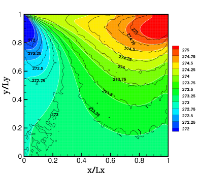
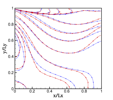
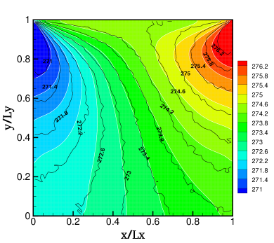
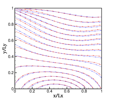
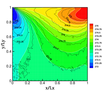
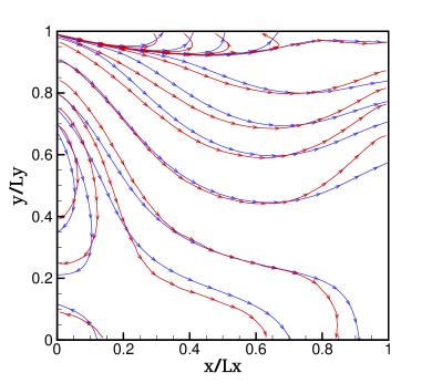
The single lid-driven cavity flow, whose configuration is shown in fig. 4a, is one of the most frequently used benchmark tests in the multi-dimensional case. Our setting is the same as in [7, 13]. To be specific, the length and height of the cavity are $L_{x}=L_{y}=$9.63\text{\times}{10}^{-7}\text{\,}\mathrm{m}$$. The top lid moves horizontally to the right with a constant speed $U_{W}=$50\text{\,}\mathrm{m}\text{/}\mathrm{s}$$ and is maintained at temperature $273\text{\,}\mathrm{K}$, while the other sides of the cavity are stationary and have the same temperature. Initially, the gas is uniformly distributed and in the Maxwellian with constant density, mean velocity of $0$, and temperature of $273\text{\,}\mathrm{K}$. Driven by the motion of the top lid, the gas would finally reach a steady state. Two initial densities given by $\rho=$0.891\text{\,}\mathrm{k}\mathrm{g}\mathrm{/}\mathrm{m}^{3}$$ and $0.0891\text{\,}\mathrm{k}\mathrm{g}\mathrm{/}\mathrm{m}^{3}$ are considered below. They correspond to the Knudsen number $0.1$ and $1.0$, respectively.

(a) Single lid-driven

(b) Four-sided lid-driven

Figure 4: Configuration of the lid-driven cavity flow problems.

4.1.1 Solution validation

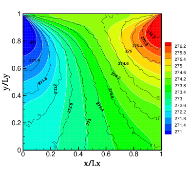
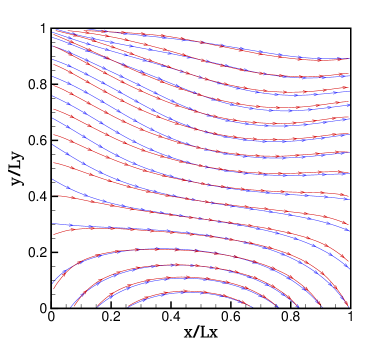
The Shakhov model is first utilized as the collision model to validate the solution of the NMG solver. Numerical solutions of the temperature and heat flux on the uniform grid with $N_{x}=N_{y}=256$ are presented, respectively, in fig. 5 for $\mathit{Kn}=0.1$, $M=20$, and in fig. 6 for $\mathit{Kn}=1.0$, $M=25$. Therein the DSMC solutions obtained in [27] are provided as a reference. It can be seen that our results agree well with the DSMC results at both Knudsen numbers, as revealed in [7], where the solution of the moment system (12) has been studied in detail. Using the NMG solver, we are in fact recovering the solution obtained in [7]. Hence we omit more discussion about the behavior of the solution here.

For the ES-BGK model, similar solutions can be obtained by the NMG solver. As an example, numerical solutions of the temperature and heat flux for the ES-BGK model, as well as the reference DSMC solutions, are shown in fig. 7 for $\mathit{Kn}=0.1$ and fig. 8 for $\mathit{Kn}=1.0$, respectively. It can be observed that for the current problem, the numerical solutions of the Shakhov model agree slightly better with the reference DSMC solutions than the numerical solutions of the ES-BGK model.

(a) Temperature $($\mathrm{K}$)$

(b) Heat flux streamlines

Figure 5: Numerical solutions of the single lid-driven flow for the Shakhov model with $\mathit{Kn}=0.1$, $M=20$, and $N_{x}\times N_{y}=256\times 256$. The black (left) and red (right) lines are the reference DSMC solutions.

(a) Temperature $($\mathrm{K}$)$

(b) Heat flux streamlines

Figure 6: Numerical solutions of the single lid-driven flow for the Shakhov model with $\mathit{Kn}=1.0$, $M=25$, and $N_{x}\times N_{y}=256\times 256$. The black (left) and red (right) lines are the reference DSMC solutions.

(a) Temperature $($\mathrm{K}$)$

(b) Heat flux streamlines

Figure 7: Numerical solutions of the single lid-driven flow for the ES-BGK model with $\mathit{Kn}=0.1$, $M=20$, and $N_{x}\times N_{y}=256\times 256$. The black (left) and red (right) lines are the reference DSMC solutions.

(a) Temperature $($\mathrm{K}$)$

(b) Heat flux streamlines

Figure 8: Numerical solutions of the single lid-driven flow for the ES-BGK model with $\mathit{Kn}=1.0$, $M=25$, and $N_{x}\times N_{y}=256\times 256$. The black (left) and red (right) lines are the reference DSMC solutions.

4.1.2 Numerical efficiency

To explore its efficiency and behavior, the NMG solver is performed with a variety of $M$ on a sequence of uniform grids for both the Shakhov and ES-BGK models. Since similar features of the NMG solver are observed for all cases, only partial results are reported in the present paper.

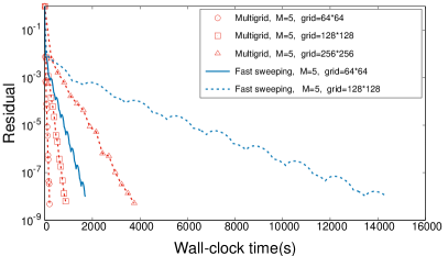
In the case of the Shakhov model, the total number of iterations and the wall-clock time, spent by the NMG solver with $M=5$ on four different grids, are listed in table 1 for $\mathit{Kn}=0.1$. For comparison, the corresponding results of two single level solvers, that is, the forward Euler scheme and the fast sweeping iteration, are also presented in table 1. Apparently, the fast sweeping iteration converges faster than the forward Euler scheme as expected. It only takes about $1/8$ of iterations of the forward Euler scheme. Benefiting from this, the wall-clock time of the fast sweeping iteration is saved to ${1}/{3}$ of that of the forward Euler scheme. Moreover, for both single level solvers, it can be also seen that roughly the total number of iterations is doubled and the wall-clock time is octupled, as the grid is refined each time, for which $N_{x}$ and $N_{y}$ are doubled. In contrast, the NMG solver behaves much better than both single level solvers by observing that it not only converges in a dozen or so iterations, but the total number of iterations is almost independent of grid size. As a result, the NMG solver becomes more and more efficient as the grid is refined. Specifically, the wall-clock time ratio of the NMG solver to the fast sweeping iteration is about $25.2\,\%$ on the grid composed of $32\times 32$ cells, whereas it is reduced drastically to $3.5\,\%$ on the grid composed of $256\times 256$ cells. In addition, some convergence histories of the NMG solver and the fast sweeping iteration are plotted in fig. 9 (left), which also shows the efficiency of the NMG solver.

Figure 9: Convergence history (left) and iterations in terms of $N_{x}\times N_{y}$ of the NMG solver (right) for the Shakhov model of single lid-driven flow with $\mathit{Kn}=0.1$.

Table 1: Performance results for the Shakhov model of single lid-driven flow with $\mathit{Kn}=0.1$ and $M=5$. Euler: the forward Euler scheme; FS: the fast sweeping iteration; NMG: the NMG solver; $T_{r}$: the wall-clock time ratio of NMG to FS.

$N_{x}\times N_{y}$	Iterations			Wall-clock time $($\mathrm{s}$)$
	Euler	FS	NMG	Euler	FS	NMG	$T_{r}$
$32\times 32$	1823	231	12	619.84	199.63	50.40	25.2 %
$64\times 64$	4100	507	12	5433.38	1701.1	199.28	11.7 %
$128\times 128$	8398	1084	13	44270.3	14373.2	875.00	6.1 %
$256\times 256$	16364	2000	14	356118	105979	3760.26	3.5 %

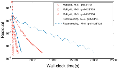
As the Knudsen number increases to $\mathit{Kn}=1.0$, the performance results of the NMG solver, as well as two single level solvers, are listed in table 2 for $M=5$. It is shown that the forward Euler scheme and the fast sweeping iteration converge more slowly and their total number of iterations increase slightly faster than the case of $\mathit{Kn}=0.1$. Yet the ratios of iterations and wall-clock time between two single level solvers seem to be preserved well. Since the NMG solver adopts the fast sweeping iteration as the smoother and the coarsest grid solver, it converges also more slowly than the case of $\mathit{Kn}=0.1$. Besides, the total number of iterations can not be maintained any more, and a few increments of it are found as the grid is refined. However, this phenomenon is acceptable in view of that the parameters such as $s_{\iota}$, $\iota=1,2,3$, are fixed in the NMG solver, and the convergence histories of the fast sweeping iteration, shown in fig. 10 (left) for $\mathit{Kn}=1.0$, fluctuate a little more in comparison to the results shown in fig. 9 (left) for $\mathit{Kn}=0.1$. What is more, the wall-clock time ratios of the NMG solver to the fast sweeping iteration, ranged from $26.5\,\%$ to $4.2\,\%$ for the grids ranged from $32\times 32$ to $256\times 256$ cells, are preserved satisfactorily as the case of $\mathit{Kn}=0.1$. Therefore, the NMG solver could be still more and more efficient as the grid is refined.

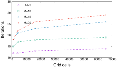
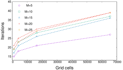
For the solvers with other $M$, the performance results for the Shakhov model on the grid composed of $64\times 64$ cells are given in table 3. It can be seen, at both Knudsen numbers, that the total number of iterations for all solvers increase gradually as $M$ grows, except for the case of $M=15$ and $\mathit{Kn}=1.0$, for which they converge faster than the case of even $M$. Actually, as mentioned in [22, 13], different behaviors with respect to the parity of $M$ have been observed for two single level solvers, and so is the NMG solver, especially in the case of $\mathit{Kn}=1.0$. Nevertheless, the acceleration of steady-state computation by using the fast sweeping iteration or the NMG solver is still prominent for all cases. Concretely, although the ratios of iterations and wall-clock time of the fast sweeping iteration to the forward Euler scheme increase for large $M$ in comparison to the case of $M=5$, it is found that the maximum ratio of wall-clock time is just about $40\,\%$. As for the NMG solver, it always converges in dozens of iterations, and the wall-clock time ratios of it to the fast sweeping iteration are around $12\,\%$ and $13\,\%$ corresponding to $\mathit{Kn}=0.1$ and $1.0$, respectively, for all $M$. Furthermore, the variations of total number of iterations for the NMG solver in terms of the grid size $N_{x}\times N_{y}$ with several choices of $M$ are plotted separately in fig. 9 (right) for $\mathit{Kn}=0.1$ and fig. 10 (right) for $\mathit{Kn}=1.0$. It is observed for each $M$ that the total number of iterations grows faster in the case of $\mathit{Kn}=1.0$ than in the case of $\mathit{Kn}=0.1$. However, since the total number of iterations would be at least doubled as the grid is refined for two single level solvers, it turns out that the efficiency of the NMG solver for steady-state computation would be more and more evident as both $N_{x}$ and $N_{y}$ increase.

Figure 10: Convergence history (left) and iterations in terms of $N_{x}\times N_{y}$ of the NMG solver (right) for the Shakhov model of single lid-driven flow with $\mathit{Kn}=1.0$.

Table 2: Performance results for the Shakhov model of single lid-driven flow with $\mathit{Kn}=1.0$ and $M=5$. Euler: the forward Euler scheme; FS: the fast sweeping iteration; NMG: the NMG solver; $T_{r}$: the wall-clock time ratio of NMG to FS.

$N_{x}\times N_{y}$	Iterations			Wall-clock time $($\mathrm{s}$)$
	Euler	FS	NMG	Euler	FS	NMG	$T_{r}$
$32\times 32$	1978	277	15	673.30	239.31	63.47	26.5 %
$64\times 64$	4952	681	18	6636.03	2284.32	303.99	13.3 %
$128\times 128$	11120	1509	21	58647.5	20003.1	1417.91	7.1 %
$256\times 256$	24266	3300	27	525312	176582	7348	4.2 %

Table 3: Performance results for the Shakhov model of single lid-driven flow with $N_{x}=N_{y}=64$. Euler: the forward Euler scheme; FS: the fast sweeping iteration; NMG: the NMG solver; $T_{r}$: the wall-clock time ratio of NMG to FS.

$\mathit{Kn}$	$M$	Iterations			Wall-clock time $($\mathrm{s}$)$
		Euler	FS	NMG	Euler	FS	NMG	$T_{r}$
0.1	10	5244	708	17	33569.5	11675.8	1401.07	12.0 %
	15	6315	875	21	116762	43611.8	5008.71	11.5 %
	20	6839	936	22	295431	114102	12596	11.0 %
1.0	10	6051	866	23	38707.2	14249.8	1892.43	13.3 %
	15	4805	702	21	88035.9	34995.3	5027.71	14.4 %
	20	6987	1008	25	301326	122825	14533.7	11.8 %

The three solvers, discussed above, also work fairly well for the ES-BGK model. As examples, the performance results on the grid composed of $64\times 64$ cells are exhibited in table 4, and the variations of total number of iterations for the NMG solver in terms of $N_{x}\times N_{y}$ with several choices of $M$ at both $\mathit{Kn}=0.1$ and $1.0$ are plotted in fig. 11. It follows that in the case of $\mathit{Kn}=0.1$, all solvers for the ES-BGK model behave almost the same as for the Shakhov model, while in the case of $\mathit{Kn}=1.0$, the forward Euler scheme requires much more iterations to guarantee convergence as $M$ increases, compared with the same case for the Shakhov model. Consequently, in this case, the fast sweeping iteration and the NMG solver converge more slowly than the counterpart solver for the Shakhov model. In spite of this, the speedup ratio of the fast sweeping iteration to the forward Euler scheme is found to be maintained, and so is the ratio of the NMG solver to the fast sweeping iteration. It is also observed from fig. 11 that the NMG solver converges in dozens of iterations even when $\mathit{Kn}=1.0$ and the grid consists of $256\times 256$. Therefore, a great improvement in efficiency can be again obtained by using the NMG solver.

At last, four results of the parallel NMG solver on the grid with $256\times 256$ cells for both Shakhov and ES-BGK models are listed in table 5, which shows a nice speedup is able to be obtained for the NMG solver by using OpenMP-based parallelization. Specifically, the speedup ratio is around $2$ and $3.7$ when, respectively, $2$ and $4$ threads are applied in parallel computation. Besides, it can be seen that the average of total number of iterations for the parallel NMG solver is almost the same as the serial NMG solver, although the details of iterations are not exactly equivalent as mentioned in section 3.3.

Table 4: Performance results for the ES-BGK model of single lid-driven flow with $N_{x}=N_{y}=64$. Euler: the forward Euler scheme; FS: the fast sweeping iteration; NMG: the NMG solver; $T_{r}$: the wall-clock time ratio of NMG to FS.

$\mathit{Kn}$	$M$	Iterations			Wall-clock time $($\mathrm{s}$)$
		Euler	FS	NMG	Euler	FS	NMG	$T_{r}$
0.1	5	4085	503	12	5138.97	1636.6	198.05	12.1 %
	10	5177	700	17	31352	10963.7	1389.26	12.7 %
	15	6357	867	21	110388	40007.2	4915.99	12.3 %
	20	6764	926	23	270399	107218	13268.6	12.4 %
1.0	5	5053	690	19	6347.05	2253.42	302.39	13.4 %
	10	7663	1105	27	46164.6	17154.5	2086.02	12.2 %
	15	5541	780	23	96388.4	36128.8	5154.89	14.3 %
	20	9177	1339	29	364166	158320	16619	10.5 %

Figure 11: Iterations in terms of $N_{x}\times N_{y}$ of the NMG solver for the ES-BGK model of single lid-driven flow with $\mathit{Kn}=0.1$ (left) and $\mathit{Kn}=1.0$ (right).

Table 5: Performance results of the parallel NMG solver with $N_{x}=N_{y}=256$ for the single lid-driven flow. $T_{r,n}$: the wall-clock time ratio of single thread to $n$ threads.

Collision model	$\mathit{Kn}$	$M$	Average iterations	Wall-clock time $($\mathrm{s}$)$ for $n$ threads
				$n=1$	$n=2$	$T_{r,2}$	$n=4$	$T_{r,4}$
Shakhov	$0.1$	$20$	30	215773	112842	1.91	59086.3	3.65
ES-BGK	$0.1$	$20$	30	209509	107997	1.94	56486.8	3.71
Shakhov	$1.0$	$25$	39	554987	277464	2.00	147878	3.75
ES-BGK	$1.0$	$25$	41	549046	276126	1.99	146859	3.74

4.2 Four-sided lid-driven cavity flow

The four-sided lid-driven cavity flow is also very important for both benchmarking and application viewpoints, and has been studied in [28]. The geometry of the anti-parallel wall motion case considered in [28] is shown in fig. 4b. That is, the top and right sides move horizontally to the right and vertically up, respectively, with a constant speed $U_{W}$, while the other two sides move in the opposite direction with the same speed relative to the motion of their parallel sides. We adopt the setting as follows. The constant speed is given by $U_{W}=$50\text{\,}\mathrm{m}\text{/}\mathrm{s}$$. All the cavity walls are maintained at temperature $273\text{\,}\mathrm{K}$. The length and height of the cavity are $L_{x}=L_{y}=$1\text{\,}\mathrm{m}$$. Initially, the gas is again assumed to be uniformly distributed and in the Maxwellian with constant density, mean velocity of $0$, and temperature of $273\text{\,}\mathrm{K}$. The initial density taken into account is $\rho=$1.1044\text{\times}{10}^{-7}\text{\,}\mathrm{k}\mathrm{g}\mathrm{/}\mathrm{m}^{3}$$. Thus the associated Knudsen number reads $\mathit{Kn}=0.777$.

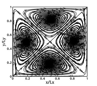
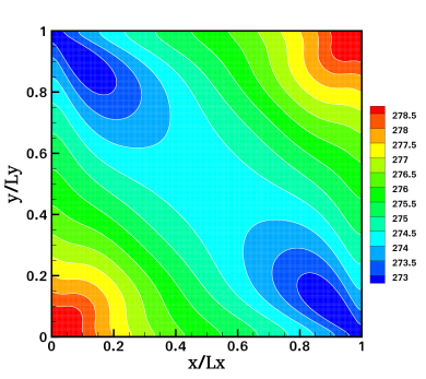
The Shakhov model is employed as the collision model for this problem. The velocity streamlines and the temperature contours obtained by the NMG solver with $M=25$ and $N_{x}=N_{y}=256$ are shown in fig. 12. These results exhibit the similar structure in comparison to the DSMC results presented in [28].

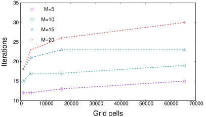
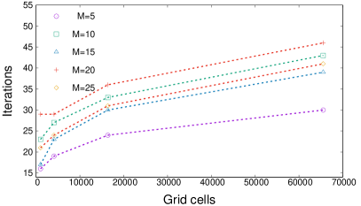
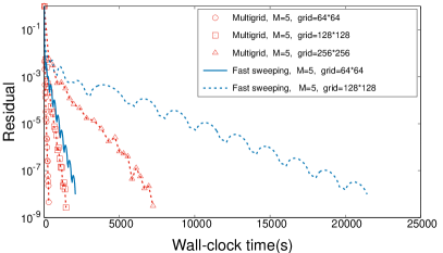
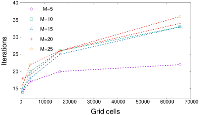
For the efficiency and behavior of the NMG solver, its results compared with the two single level solvers on the grid composed of $64\times 64$ cells for a variety of $M$ are listed in table 6. As can be seen once more, the fast sweeping iteration converges faster than the forward Euler scheme for all $M$, so that the wall-clock time is saved a lot in steady-state computation. For the NMG solver, it converges within $20$ iterations for all cases, resulting in the wall-clock time ratios of it to the fast sweeping iteration being around $13\,\%$. When the grid is refined, several convergence histories of the NMG solver and the fast sweeping iteration for $M=5$, and the variations of total number of iterations for the NMG solver with five values of $M$ are presented in fig. 13. These results are enough to show the wonderful efficiency and behavior of the NMG solver. Additionally, the efficiency in steady-state computation could be further improved with a nice speedup ratio by using the parallel NMG solver, according to the results shown in table 7.

(a) Velocity streamlines

(b) Temperature $($\mathrm{K}$)$

Figure 12: Numerical solutions of the four-sided lid-driven flow for the Shakhov model with $M=25$ and $N_{x}\times N_{y}=256\times 256$.

Figure 13: Convergence history (left) and iterations in terms of $N_{x}\times N_{y}$ of the NMG solver (right) for the Shakhov model of four-sided lid-driven flow.

Table 6: Performance results for the Shakhov model of four-sided lid-driven flow with $N_{x}=N_{y}=64$. Euler: the forward Euler scheme; FS: the fast sweeping iteration; NMG: the NMG solver; $T_{r}$: the wall-clock time ratio of NMG to FS.

$M$	Iterations			Wall-clock time $($\mathrm{s}$)$
	Euler	FS	NMG	Euler	FS	NMG	$T_{r}$
5	4442	607	17	6031.19	2068.4	295.75	14.3 %
10	4565	661	20	29037.5	12436.3	1693.24	13.6 %
15	3783	621	18	71309.2	32209.3	4319.35	13.4 %
20	5731	831	19	238658	103063	12709	12.3 %

Table 7: Performance results of the parallel NMG solver with $N_{x}=N_{y}=256$ in sections 4.2 and 4.3. $T_{r,n}$: the wall-clock time ratio of single thread to $n$ threads.

Subsection	$\mathit{Kn}$	$M$	Average iterations	Wall-clock time $($\mathrm{s}$)$ for $n$ threads
				$n=1$	$n=2$	$T_{r,2}$	$n=4$	$T_{r,4}$
4.2	$0.777$	$25$	37	522770	266148	1.96	142230	3.68
4.3	$0.3$	$20$	26	201206	102487	1.96	53074.4	3.79

4.3 Heat transfer in a bottom-heated cavity

The third example is a heat transfer problem for the rarefied gas confined in a bottom-heated cavity. As in [29, 13], all sides of the cavity are stationary and kept at temperature $300\text{\,}\mathrm{K}$, except for the bottom side, which is kept at temperature $600\text{\,}\mathrm{K}$. The length and height of the cavity are taken as $L_{x}=L_{y}=${10}^{-6}\text{\,}\mathrm{m}$$, and the initial density, corresponding to the Knudsen number $0.3$, is set to $0.2733\text{\,}\mathrm{k}\mathrm{g}\mathrm{/}\mathrm{m}^{3}$. In addition, all the computations start from the initial global Maxwellian with the given density, mean velocity of $0$, and temperature of $300\text{\,}\mathrm{K}$.

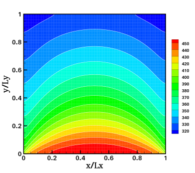
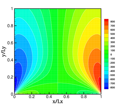
Numerical solutions of the temperature and shear stress obtained by the NMG solver for the Shakhov model with $M=20$ and $N_{x}=N_{y}=256$ are plotted in fig. 14. Compared with the results presented in [13], it appears that the NMG solver for the Shakhov model gives a reasonable distribution of the temperature and shear stress.

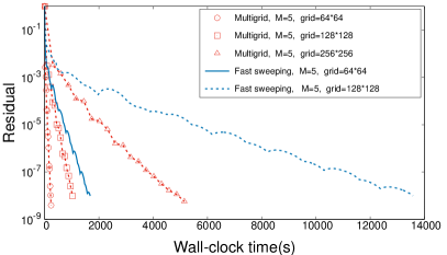
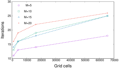
Then, the performance of the NMG solver for the above problem, compared with the two single level solvers, is investigated. The results on the grid with $64\times 64$ cells for several choices of $M$ are presented in table 8. With these values of $M$, the variations of total number of iterations for the NMG solver with respect to $N_{x}\times N_{y}$, as well as their partial convergence histories, are shown in fig. 15. For the speedup of simulation by using the parallel NMG solver, it can be found in table 7. From all of these results, we deduce that the NMG solver performs analogously as in the previous examples. That is, the NMG solver always converges in dozens of iterations. Consequently, compared with the fast sweeping iteration, which is already more efficient than the forward Euler scheme, the NMG solver is able to accelerate the steady-state computation more significantly, especially in the case that the number of grid cells is large. When multi-threads are applied, the parallel NMG solver would further accelerate the simulation with a pretty speedup ratio.

(a) Temperature $($\mathrm{K}$)$

(b) Shear stress $($\mathrm{Pa}$)$

Figure 14: Numerical solutions of the bottom-heated flow for the Shakhov model with $M=20$ and $N_{x}\times N_{y}=256\times 256$.

Figure 15: Convergence history (left) and iterations in terms of $N_{x}\times N_{y}$ of the NMG solver (right) for the Shakhov model of bottom-heated flow.

Table 8: Performance results for the Shakhov model of bottom-heated flow with $N_{x}=N_{y}=64$. Euler: the forward Euler scheme; FS: the fast sweeping iteration; NMG: the NMG solver; $T_{r}$: the wall-clock time ratio of NMG to FS.

$M$	Iterations			Wall-clock time $($\mathrm{s}$)$
	Euler	FS	NMG	Euler	FS	NMG	$T_{r}$
5	4073	499	13	5668.54	1677.59	236.72	15.7 %
10	4926	589	16	31041.7	9739.9	1404.25	14.4 %
15	5357	664	16	100517	33575.4	4039.22	12.0 %
20	5991	745	19	253515	93542.3	10999.1	11.8 %

4.4 Second-order spatial discretization for single lid-driven cavity flow

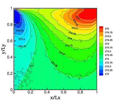
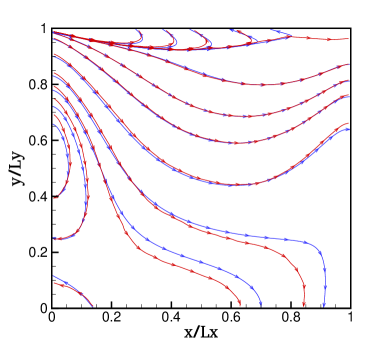
In the last subsection, the NMG solver for the second-order spatial discretization is investigated by recomputing the single lid-driven cavity flow. The Shakhov model and the Knudsen number $\mathit{Kn}=0.1$ are applied. Numerical solutions of the temperature and heat flux for $M=20$ and $N_{x}=N_{y}=128$, together with the reference DSMC solutions, are presented in fig. 16. As anticipated, we can observe that the temperature contours and heat flux streamlines using the second-order spatial discretization on a coarser grid with $128\times 128$ cells coincide with the DSMC results much better than the results using the first-order spatial discretization on the grid with $256\times 256$ cells that are shown in fig. 5, especially in the region near the boundary.

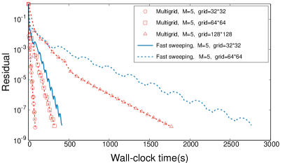
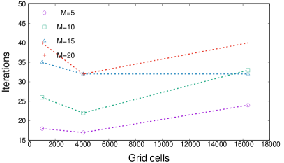
For the second-order spatial discretization, it has been observed in our simulation that the forward Euler scheme fails to converge due to instability, while the fast sweeping iteration still works well so that the NMG solver using it as the smoother is able to give satisfactory results too. In table 9, the total number of iterations and the wall-clock time, spent by the NMG solver and the fast sweeping iteration for the second-order spatial discretization in the case of $M=5$ on three grids, are listed. Compared with the results shown in table 1 for the first-order spatial discretization, it turns out that, on the same grid, the fast sweeping iteration converges more slowly for second-order case, whereas as the grid is refined, the resulting total number of iterations increases with a better growth rate for second-order case. Meanwhile, the NMG solver also behaves somewhat differently from the first-order case. It can be seen from table 9 as well as fig. 17 (right) that the total number of iterations of the NMG solver for almost all $M$ decreases first and then increases on the three grids ranged from $32\times 32$ to $128\times 128$ cells. For more details, it can be found from fig. 17 (left) that, due to the fluctuation of residuals generated by the smoother, i.e., the fast sweeping iteration, the convergence history of the NMG solver on the smallest grid fluctuates a little more than that on the other grids. Apart from this, the convergence rate of the NMG solver on the finest grid appears to be degenerate slightly after a few number of iterations. As a result, a little more iterations to obtain the steady state are spent by the NMG solver on these grids than on the middle grid.

Nevertheless, we still have that the NMG solver converges in dozens of iterations for all simulations, so that it could improve the efficiency remarkably in steady-state computation. Additionally, it is clear from table 10 that the expected speedup could be further obtained by using the NMG solver with multi-threads.

(a) Temperature $($\mathrm{K}$)$

(b) Heat flux streamlines

Figure 16: Numerical solutions of the single lid-driven flow for the Shakhov model with $\mathit{Kn}=0.1$, $M=20$, $N_{x}\times N_{y}=128\times 128$, and second-order spatial discretization. The black (left) and red (right) lines are the reference DSMC solutions.

Figure 17: Convergence history (left) and iterations in terms of $N_{x}\times N_{y}$ of the NMG solver (right) for the Shakhov model of single lid-driven flow with $\mathit{Kn}=0.1$, and second-order spatial discretization.

Table 9: Performance results for the Shakhov model of single lid-driven flow with $\mathit{Kn}=0.1$, $M=5$ and second-order spatial discretization. FS: the fast sweeping iteration; NMG: the NMG solver; $T_{r}$: the wall-clock time ratio of NMG to FS.

$N_{x}\times N_{y}$	Iterations		Wall-clock time $($\mathrm{s}$)$
	FS	NMG	FS	NMG	$T_{r}$
$32\times 32$	384	18	412.78	82.80	20.1 %
$64\times 64$	728	17	2761.07	320.25	11.6 %
$128\times 128$	1331	24	19393.3	1769.73	9.1 %

Table 10: Performance results of the parallel NMG solver for the Shakhov model of single lid-driven flow with $\mathit{Kn}=0.1$, $M=20$ and second-order spatial discretization. $T_{r,n}$: the wall-clock time ratio of single thread to $n$ threads.

$N_{x}\times N_{y}$	Average iterations	Wall-clock time $($\mathrm{s}$)$ for $n$ threads
		$n=1$	$n=2$	$T_{r,2}$
$64\times 64$	36	19307.8	11485.8	1.68
$128\times 128$	40	81154.8	41326.2	1.96

5 Conclusion

Aiming at efficient steady-state simulation of rarefied gas cavity flow described by the Boltzmann equation with BGK-type collision term, a nonlinear multigrid solver has been successfully developed based on the following approaches. At first, it adopts the unified framework of regularized moment method for velocity discretization and finite volume method for spatial discretization. To solve the resulting discrete problem, a fast sweeping iteration that converges faster and more robust than the time-integration scheme is introduced. Then, the NMG method, which employs the fast sweeping iteration as the smoother, is proposed to greatly improve the convergence rate. Finally, the OpenMP-based parallelization is applied for the implementation of the NMG method, so that the efficiency could be further improved by multi-threaded parallel computation. Plenty of numerical experiments have been carried out to investigate the performance of the resulting NMG solver. All numerical results show the efficiency and robustness of the solver for both first- and second-order spatial discretization.

Incidentally, it is easy to extend the proposed NMG solver to the Boltzmann equation with other collision models by providing the computation of the coefficients $Q_{ij,\alpha}$ in 14. Indeed, combining the algorithm presented in [31], the performance of the NMG solver for the Boltzmann equation with the quadratic collision term is under investigation and will be reported elsewhere.

References

- [1] P. L. Bhatnagar, E. P. Gross, and M. Krook. A model for collision processes in gases. I. small amplitude processes in charged and neutral one-component systems. Phys. Rev., 94(3):511–525, 1954.
- [2] A. Brandt. Multi-level adaptive solutions to boundary-value problems. Math. Comp., 31(138):333–390, 1977.
- [3] A. Brandt and O. E. Livne. Multigrid Techniques: 1984 Guide with Applications to Fluid Dynamics. Classics in Applied Mathematics. SIAM, revised edition, 2011.
- [4] Z. Cai. Moment method as a numerical solver: Challenge from shock structure problems. J. Comput. Phys., 444:110593, 2021.
- [5] Z. Cai, Y. Fan, and R. Li. Globally hyperbolic regularization of Grad’s moment system. Comm. Pure Appl. Math., 67(3):464–518, 2014.
- [6] Z. Cai, Y. Fan, and R. Li. A framework on moment model reduction for kinetic equation. SIAM J. Appl. Math., 75(5):2001–2023, 2015.
- [7] Z. Cai, Y. Fan, R. Li, and Z. Qiao. Dimension-reduced hyperbolic moment method for the Boltzmann equation with BGK-type collision. Commun. Comput. Phys., 15(5):1368–1406, 2014.
- [8] Z. Cai, Y. Fan, and Y. Wang. Burnett spectral method for the spatially homogeneous Boltzmann equation. Comput. Fluids, 200:104456, 2020.
- [9] Z. Cai and R. Li. Numerical regularized moment method of arbitrary order for Boltzmann-BGK equation. SIAM J. Sci. Comput., 32(5):2875–2907, 2010.
- [10] Z. Cai, R. Li, and Z. Qiao. NR simulation of microflows with Shakhov model. SIAM J. Sci. Comput., 34(1):A339–A369, 2012.
- [11] Z. Cai, R. Li, and Z. Qiao. Globally hyperbolic regularized moment method with applications to microflow simulation. Comput. Fluids, 81:95–109, 2013.
- [12] Z. Cai, R. Li, and Y. Wang. An efficient NR method for Boltzmann-BGK equation. J. Sci. Comput., 50(1):103–119, 2012.
- [13] Z. Cai and M. Torrilhon. Numerical simulation of microflows using moment methods with linearized collision operator. J. Sci. Comput., 74:336–374, 2018.
- [14] Z. Cai and M. Torrilhon. On the Holway-Weiss debate: Convergence of the Grad-moment-expansion in kinetic gas theory. Phys. Fluids, 31:126105, 2020.
- [15] L. Dagum and R. Menon. OpenMP: an industry standard API for shared-memory programming. IEEE Comput. Sci. Eng., 5(1):46–55, 1998.
- [16] I. M. Gamba, J. R. Haack, C. D. Hauck, and J. Hu. A fast spectral method for the Boltzmann collision operator with general collision kernels. SIAM J. Sci. Comput., 39(14):B658–B674, 2017.
- [17] H. Grad. On the kinetic theory of rarefied gases. Comm. Pure Appl. Math., 2(4):331–407, 1949.
- [18] W. Hackbusch. Multi-Grid Methods and Applications. Springer-Verlag, Berlin, 1985. second printing 2003.
- [19] L. H. Holway. New statistical models for kinetic theory: Methods of construction. Phys. Fluids, 9(1):1658–1673, 1966.
- [20] Z. Hu and Z. Cai. Burnett spectral method for high-speed rarefied gas flows. SIAM J. Sci. Comput., 42(5):B1193–B1226, OCT 2020.
- [21] Z. Hu, Z. Cai, and Y. Wang. Numerical simulation of microflows using Hermite spectral methods. SIAM J. Sci. Comput., 42(1):B105–B134, 2020.
- [22] Z. Hu and G. Hu. An efficient steady-state solver for microflows with high-order moment model. J. Comput. Phys., 392:462–482, SEP 2019.
- [23] Z. Hu and R. Li. A nonlinear multigrid steady-state solver for 1D microflow. Comput. Fluids, 103:193–203, 2014.
- [24] Z. Hu, R. Li, and Z. Qiao. Acceleration for microflow simulations of high-order moment models by using lower-order model correction. J. Comput. Phys., 327:225–244, DEC 2016.
- [25] Z. Hu, R. Li, and Z. Qiao. Extended hydrodynamic models and multigrid solver of a silicon diode simulation. Commun. Comput. Phys., 20(3):551–582, Sep 2016.
- [26] T. Imamura, K. Suzuki, T. Nakamura, and M. Yoshida. Acceleration of steady-state lattice Boltzmann simulations on non-uniform mesh using local time step method. J. Comput. Phys., 202(2):645–663, Jan 2005.
- [27] B. John, X.-J. Gu, and D. R. Emerson. Investigation of heat and mass transfer in a lid-driven cavity under nonequilibrium flow conditions. Numer. Heat Transfer, Part B, 58(5):287–303, 2010.
- [28] D. Nabapure and R. C. Murthy K. DSMC investigation of rarefied gas flow in a four-sided lid driven cavity: Effect of rarefaction and lid velocities. J. Comput. Sci., 49:101276, 2021.
- [29] A. S. Rana, A. Mohammadzadeh, and H. Struchtrup. A numerical study of the heat transfer through a rarefied gas confined in a microcavity. Continuum Mech. Thermodyn., 27:433–446, 2015.
- [30] E. M. Shakhov. Generalization of the Krook kinetic relaxation equation. Fluid Dyn., 3(5):95–96, 1968.
- [31] Y. Wang and Z. Cai. Approximation of the Boltzmann collision operator based on Hermite spectral method. J. Comput. Phys., 397:108815, 2019.
- [32] L. Wu, C. White, T. Scanlona, J. Reese, and Y. Zhang. Deterministic numerical solutions of the Boltzmann equation using the fast spectral method. J. Comput. Phys., 250:27–52, 2013.
- [33] L. Wu, Y.-T. Zhang, S. Zhang, and C.-W. Shu. High order fixed-point sweeping WENO methods for steady state of hyperbolic conservation laws and its convergence study. Commun. Comput. Phys., 20(04):835–869, 2016.
- [34] L.M. Yang, X. Zhao, C. Shu, and Y.J. Du. Parametric reduced order modeling-based discrete velocity method for simulation of steady rarefied flows. J. Comput. Phys., 430:110037, 2021.
- [35] L. Zhu, X. Pi, W. Su, Z.-H. Li, Y. Zhang, and L. Wu. General synthetic iterative scheme for nonlinear gas kinetic simulation of multi-scale rarefied gas flows. J. Comput. Phys., 430:110091, 2021.