BYOL-Explore:
Exploration by Bootstrapped Prediction

Abstract

We present BYOL-Explore, a conceptually simple yet general approach for curiosity-driven exploration in visually-complex environments. BYOL-Explore learns a world representation, the world dynamics, and an exploration policy all-together by optimizing a single prediction loss in the latent space with no additional auxiliary objective. We show that BYOL-Explore is effective in DM-HARD-8, a challenging partially-observable continuous-action hard-exploration benchmark with visually-rich $3$-D environments. On this benchmark, we solve the majority of the tasks purely through augmenting the extrinsic reward with BYOL-Explore’s intrinsic reward, whereas prior work could only get off the ground with human demonstrations. As further evidence of the generality of BYOL-Explore, we show that it achieves superhuman performance on the ten hardest exploration games in Atari while having a much simpler design than other competitive agents.

1 Introduction

Exploration is essential to reinforcement learning (RL) [65], especially when extrinsic rewards are sparse or hard to reach. In rich environments, the variety of meaningful directions of exploration makes it impractical to visit everything. Thus, the question becomes: how can an agent determine which parts of the environment are interesting to explore? One promising paradigm to address this challenge is curiosity-driven exploration. It consists of (i) learning a predictive model of some information about the world, called a world model, and (ii) using discrepancies between predictions of the world model and real experience to build intrinsic rewards [58, 64, 59, 34, 50, 51, 2]. An RL agent optimizing these intrinsic rewards drives itself towards states where the world model is incorrect or imperfect, generating new trajectories on which the world model can be improved. In other words, the properties of the world model influence the quality of the exploration policy, which in turn gathers new data to shape the world model itself. Thus, it can be important not to treat learning the world model and learning the exploratory policy as two separate problems, but instead altogether as a single joint problem to solve.

In this paper, we present BYOL-Explore, a curiosity-driven exploration algorithm whose appeal resides in its conceptual simplicity, generality, and high performance. BYOL-Explore learns a world model with a self-supervised prediction loss, and uses the same loss to train a curiosity-driven policy, thus using a single learning objective to solve both the problem of building the world model’s representation and the curiosity-driven policy. Our approach builds upon Bootstrap Your Own Latent (BYOL), a latent-predictive self-supervised method which predicts an older copy of its own latent representation. This bootstrapping mechanism has already been successfully applied in computer vision [21, 55], graph representation learning [69], and representation learning in RL [24, 61]. However, the latter works focus primarily on using the world-model for representation learning in RL whereas BYOL-Explore takes this one step further, and not only learns a versatile world model but also uses the world model’s loss to drive exploration.

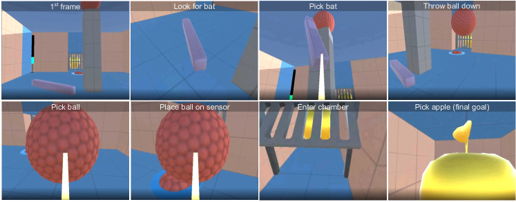
We evaluate BYOL-Explore on DM-HARD-8 [22], a suite of $8$ complex first-person-view $3$-D tasks with sparse rewards. These tasks demand efficient exploration since in order to reach the final goal and obtain the reward they require completing a sequence of precise, orderly interactions with the physical objects in the environment, unlikely to happen under a vanilla random exploration strategy (see Fig. 2 and videos). To show the generality of our method we also evaluate BYOL-Explore on the ten hardest exploration Atari games [6]. In all these domains, BYOL-Explore outperforms other prominent curiosity-driven exploration methods, such as Random Network Distillation (RND) [9] and Intrinsic Curiosity Module (ICM) [50]. In DM-HARD-8, BYOL-Explore achieves human-level performance in the majority of the tasks using only the extrinsic reward augmented with BYOL-Explore’s intrinsic reward, whereas previously significant progress required human demonstrations [22]. Remarkably, BYOL-Explore achieves this performance using only a single world model and a single policy network concurrently trained across all tasks. Finally, as further evidence of its generality, BYOL-Explore achieves superhuman performance in the ten hardest exploration Atari games [6] while having a simpler design than other competitive agents, such as Agent57 [4, 5] and Go-Explore [15, 16].

2 Related Work

There is a large body of research in building world models either for planning [64, 62, 27, 26, 60], representation learning [61, 24, 41, 20] or curiosity-driven exploration [58, 66, 59, 34, 50, 51, 2, 62]. Most works consider world models that predict the entire observations [57, 47, 17, 20], which necessitates a loss in pixel space when observations are visually complex images. Some works have considered predicting latent representations, whether they are random projections [8, 9], or learned representations from a separate model, such as an inverse dynamics model [50] or an auto-encoder [25, 8]. Finally, some RL works [60] have focused on predicting lower-dimensional quantities such as the extrinsic reward, the action-selection policy, and the value function to build a world model.

Our BYOL-Explore’s world model operates in latent space and uses the same loss both for representation and intrinsic reward, simplifying and unifying representation learning and exploration. BYOL-Explore’s world model is derived from recent self-supervised representation learning methods [21, 55, 54, 69] and is similar to the ones in self-supervised RL [61, 24]. These previous works focused on the benefit of shaping representations for policy learning and have not looked into exploration. We build on this previous work to show that we can take the impact of a good representation technique further and use it to drive exploration.

While our approach belongs to the curiosity-driven exploration paradigm [49, 42, 48, 58, 6, 66, 59, 34, 50, 51, 2, 62], other exploration paradigms have also been proposed. The maximum entropy paradigms try to steer the agent to a desired distribution of states (or state-action pairs) that maximizes the entropy of visited states [29, 67, 68, 23]. The goal-conditioned paradigm has the agent set its own goal drive exploration [56, 1, 18, 73, 46, 13, 80, 28, 16, 53, 78, 52]. The reward-free exploration paradigm consists of training an agent to explore the environment such that it would be able to produce a near-optimal policy for any possible reward function [37, 39, 44, 76, 72, 10, 77, 79].

3 Method

Our agent has three components: a self-supervised latent-predictive world-model called BYOL-Explore, a generic reward normalization and prioritization scheme, and an off-the-shelf RL agent that can optionally share its own representation with BYOL-Explore’s world model.

3.1 Background and Notation

We consider a discrete-time interaction process [43, 35, 36, 14] between an agent and its environment where, at each time step $t\in\mathbb{N}$, the agent receives an observation $o_{t}\in\mathcal{O}$ and generates an action $a_{t}\in\mathcal{A}$. We consider an environment with stochastic dynamics $p:\mathcal{H}\times\mathcal{A}\rightarrow\Delta_{\mathcal{O}}$ that maps a history of past observations-actions and a current action to a probability distribution over future observations. More precisely, the space of past observations-actions is $\mathcal{H}=\bigcup_{t\in\mathbb{N}}\mathcal{H}_{t}$ where $\mathcal{H}_{0}=\mathcal{O}$ and $\forall t\in\mathbb{N}^{*},\mathcal{H}_{t+1}=\mathcal{H}_{t}\times\mathcal{A}\times\mathcal{O}$. We consider policies $\pi:\mathcal{H}\rightarrow\Delta_{\mathcal{A}}$ that maps a history of past observations-actions to a probability distribution over actions. Finally, an extrinsic reward function $r_{e}:\mathcal{H}\times\mathcal{A}\rightarrow\mathbb{R}$ maps a history of past observations-actions to a real number.

3.2 Latent-Predictive World Model

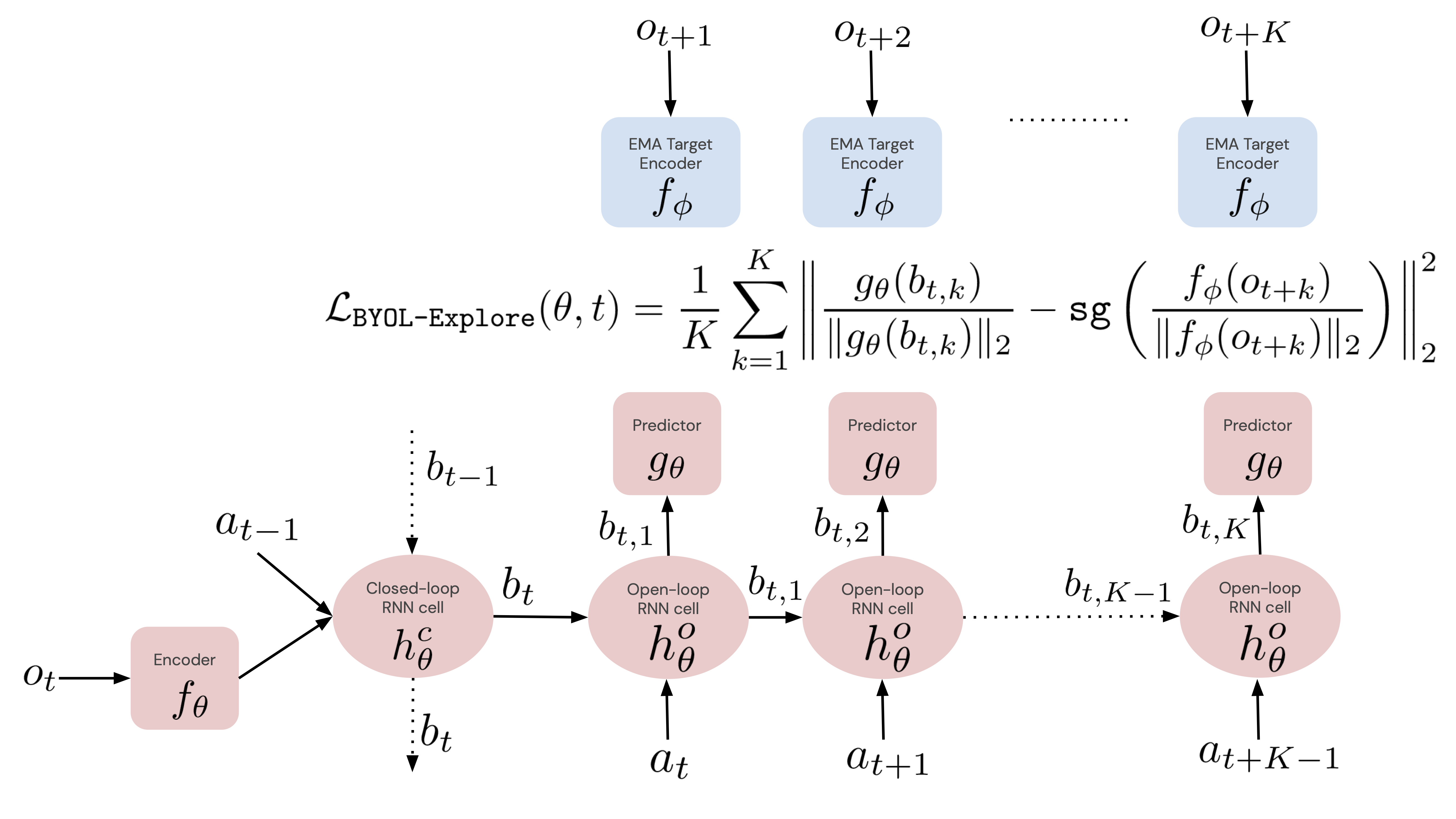
BYOL-Explore world model is a multi-step predictive world model operating at the latent level. It is inspired by the self-supervised learning method BYOL in computer vision and adapted to interactive environments (see Section 3.1). Similar to BYOL, BYOL-Explore model trains an online network using targets generated by an exponential moving average (EMA) target network. However, BYOL obtains its targets by applying different augmentations to the same observation as the online representation, whereas BYOL-Explore model gets its targets from future observations processed by an EMA of the online network, with no hand-crafted augmentation. Also BYOL-Explore model, uses a recurrent neural network (RNN) [33, 12] to build the agent state, i.e., the state of RNN, from the history of observations, whereas the original BYOL only uses a feed-forward network for encoding the observations. In the remainder of this section, we will explain: (i) how the online network builds future predictions, (ii) how targets for our predictions are obtained through a target network, (iii) the loss used to train the online network, and (iv) how we compute the uncertainties of the world model.

Figure 1: BYOL-Explore’s Neural Architecture (see main text for details).

(i) Future Predictions.

The online network is composed of an encoder $f_{\theta}$ that transforms an observation $o_{t}$ into an observation-representation $f_{\theta}(o_{t})\in\mathbb{R}^{N}$, where $N\in\mathbb{N^{*}}$ is the embedding size. The observation-representation $f_{\theta}(o_{t})$ is then fed alongside the previous action $a_{t-1}$ to a RNN cell $h^{c}_{\theta}$ that is referred as the close-loop RNN cell. It computes a representation $b_{t}\in\mathbb{R}^{M}$ of the history $h_{t}\in\mathcal{H}_{t}$ seen so far as $b_{t}=h^{c}_{\theta}(b_{t-1},a_{t-1},f_{\theta}(o_{t}))$, where $M\in\mathbb{N}^{*}$ is the size of the history-representation. Then, the history-representation $b_{t}$ is used to initialize an open-loop RNN cell $h^{o}_{\theta}$ that outputs open-loop representations $(b_{t,k}\in\mathbb{R}^{M})_{k=1}^{K-1}$ as $b_{t,k}=h^{o}_{\theta}(b_{t,k-1},a_{t+k-1})$ where $b_{t,0}=b_{t}$ and $K$ is the open-loop horizon. The role of the open-loop RNN cell is to simulate future history-representations while observing only the future actions. Finally, the open-loop representation $b_{t,k}$ is fed to a predictor $g_{\theta}$ to output the open-loop prediction $g_{\theta}(b_{t,k})\in\mathbb{R}^{N}$ at time $t+k$ that plays the role of our future prediction at time $t+k$.

(ii) Targets and Target Network.

The target network is an observation encoder $f_{\phi}$ whose parameters are an EMA of the online network’s parameters $\theta$. It outputs targets $f_{\phi}(o_{t+k})\in\mathbb{R}^{N}$ that are used to train the online network. After each training step, the target network’s weights are updated via an EMA update $\phi\leftarrow\alpha\phi+(1-\alpha)\theta$ where $\alpha$ is the target network EMA parameter. A sketch of the neural architecture is provided in Fig. 1, with more details in App. A.

(iii) Online Network Loss Function.

Suppose our RL agent collected a batch of trajectories $\mathopen{}\mathclose{{}\left((o^{j}_{t},a^{j}_{t})_{t=0}^{T-1}}\right)_{j=0}^{B-1}$, where $T\in\mathbb{N}^{*}$ is the trajectory length and $B\in\mathbb{N}^{*}$ is the batch size. Then, the loss $\mathcal{L}_{\texttt{BYOL-Explore}}(\theta)$ to minimize is defined as the average cosine distance between the open-loop future predictions $g_{\theta}(b^{j}_{t,k})$ and their respective targets $f_{\phi}(o^{j}_{t+k})$ at time $t+k$:

$$\mathcal{L}_{\texttt{BYOL-Explore}}(\theta,j,t,k) =\mathopen{}\mathclose{{}\left\|\frac{g_{\theta}(b^{j}_{t,k})}{\|g_{\theta}(b^{j}_{t,k})\|_{2}}-\texttt{sg}\mathopen{}\mathclose{{}\left(\frac{f_{\phi}(o^{j}_{t+k})}{\|f_{\phi}(o^{j}_{t+k})\|_{2}}}\right)}\right\|_{2}^{2},$$

$$\mathcal{L}_{\texttt{BYOL-Explore}}(\theta) =\frac{1}{B(T-1)}\sum_{j=0}^{B-1}\sum_{t=0}^{T-2}\frac{1}{K(t)}\sum_{k=1}^{K(t)}\mathcal{L}_{\texttt{BYOL-Explore}}(\theta,j,t,k),$$

where $K(t)=\min(K,T-1-t)$ is the valid open-loop horizon for a trajectory of length $T$ and sg is the stop-gradient operator.

(iv) World Model Uncertainties

The uncertainty associated to the transition $(o^{j}_{t},a^{j}_{t},o^{j}_{t+1})$ is the sum of the corresponding prediction losses:

$$\ell^{\,j}_{t}=\sum_{p+q=t+1}\mathcal{L}_{\texttt{BYOL-Explore}}(\theta,j,p,q),$$

where $0\leq p\leq T-2$, $1\leq q\leq K$ and $0\leq t\leq T-2$. This accumulates all the losses corresponding to the world-model uncertainties relative to the observation $o^{j}_{t+1}$. Thus, a timestep receives intrinsic reward based on how difficult its observation was to predict from past partial histories.

Intuition on why BYOL-Explore learns a meaningful representation.

The intuition behind BYOL-Explore is similar in spirit to the one behind BYOL. In early training, the target network is initialized randomly, and so BYOL-Explore’s online network and the closed-loop RNN are trained to predict random features of the future. This encourages the online observation representation to capture information that is useful to predict the future. This information is then distilled into the target observation encoder network through the EMA slow copy mechanism. In turn, these features become targets for the online network and predicting them can further improve the quality of the online representation. For further theoretical and empirical insights on why the bootstrap latent methods learn non-trivial representations see, e.g., [70, 74].

3.3 Reward Normalization and Prioritization Scheme

Reward Normalization.

We use the world model uncertainties $\ell^{\,j}_{t}$ as an intrinsic reward. To counter the non-stationarity of the uncertainties during training, we adopt the same reward normalization scheme as RND [9] and divide the raw rewards $((\ell^{\,j}_{t})_{t=0}^{T-2})_{j=0}^{B-1}$ by an EMA estimate of their standard deviation $\sigma_{r}$. The normalized rewards are $\ell^{\,j}_{t}/\sigma_{r}$. Details are provided in App. A.3.

Reward Prioritization.

In addition to normalizing the rewards, we can optionally prioritize them by optimizing only the rewards with highest uncertainties and nullifying rewards with the lowest uncertainties. Because of the transient nature of the intrinsic rewards, this allows the agent to focus first on parts of the environment where the model is not accurate. Later on, if the previously nullified rewards remain, they will naturally become the ones with highest uncertainties and be optimized. This mechanism allows the agent to optimize only the source of high uncertainties and not optimize all sources of uncertainties at once. To do so, let us denote by $\mu_{\ell/\sigma_{r}}$ the adjusted EMA mean relative to the successive batch of normalized rewards $((\ell^{\,j}_{t}/\sigma_{r})_{t=0}^{T-2})_{j=0}^{B-1}$. We use $\mu_{\ell/\sigma_{r}}$ as a clipping threshold separating high and low-uncertainty rewards. Then, the clipped and normalized reward that plays the role of intrinsic reward is: $r^{j}_{i,t}=\max(\ell^{\,j}_{t}/\sigma_{r}-\mu_{\ell/\sigma_{r}},0)\cdot$

3.4 Generic RL Algorithm and Representation Sharing

BYOL-Explore can be used in conjunction with any RL algorithm for training the policy. In addition to providing an intrinsic reward, BYOL-Explore can further be used to shape the representation learnt by the RL agent by directly sharing some components of the BYOL-Explore world model with the RL model. For instance, consider a recurrent agent composed of an encoder $f_{\psi}$, an RNN cell $h^{c}_{\psi}$, a policy head $\pi_{\psi}$ and a value head $v_{\psi}$ that are shaped by an RL loss. Then, we can share the weights $\theta$ of the BYOL-Explore world model and the weights $\psi$ of the RL model at the level of the encoder and the RNN cell: $f_{\psi}=f_{\theta}$ and $h^{c}_{\theta}=h^{c}_{\psi}$ and let the joint representation be trained via both the RL loss and BYOL-Explore. In our experiments, we will show results for both the shared and unshared settings. Architectural details are provided in Appendix A.

4 Experiments

We evaluate the algorithms on benchmark task-suites known to contain hard exploration challenges. These benchmarks have different properties in terms of the complexity of the observations, partial observability, and procedural generation, allowing us to test the generality of our approach. Our agents are implemented in the JAX ecosystem of libraries [3].

Atari Learning Environment [7].

This is a widely used RL benchmark, comprising of approximately $50$ Atari games. These are $2$-D, fully-observable, (fairly) deterministic environments for most of the games but have a very long optimization horizon (episodes last for an average of $10000$ steps) and complex observations (preprocessed greyscale images which are $84\times 84$ byte arrays). We select the $10$ hardest exploration games [6] to conduct our experiments: Alien, Freeway, Gravitar, Hero, Montezuma’s Revenge, Pitfall, Private Eye, Qbert, Solaris and Venture.

Hard-Eight Suite [22].

This benchmark comprises of $8$ hard exploration tasks, originally built to emphasize the difficulties encountered by an RL agent when learning from sparse rewards in a procedurally-generated $3$-D world with partial observability, continuous control, and highly variable initial conditions. Each task requires the agent to interact with specific objects in its environment in order to reach a large apple that provides reward (see Fig. 2). Being procedurally-generated, properties such as object shapes, colors, and positions are different every episode. The agent sees only the first-person view from its position; but for greater clarity we provide videos showing top-down view and a third-person view as well to ground the difficulty of these tasks. Note that the current best RL agents that solve these tasks require a small (but non-zero) amount of human expert demonstrations. Without demonstrations or reward shaping, state-of-the-art deep RL algorithms, such as R2D2 [38], do not get positive reward signal on any of the tasks. In our case, we train a single RL agent and a single world model to tackle the 8 tasks all-together, making for a challenging multi-task setting.

Figure 2: $1^{\text{st}}$-person-view snapshots of the human player solving Baseball task. They are ordered chronologically from left to right and top to bottom. Each image depicts a specific stage of the task.

4.1 Experimental Setup

At a high level, BYOL-Explore has $4$ main hyper-parameters: the target network EMA parameter $\alpha$, the open-loop horizon $K$, choosing to clip rewards and to share the BYOL-Explore representation with the RL network. To better understand what part of BYOL-Explore is essential to perform well, we run $4$ ablations. Each ablation corresponds to BYOL-Explore where only one hyper-parameter has been changed. The $4$ ablations are namely Fixed-targets where the target network EMA parameter is set to $\alpha=1$, Horizon=1 where the horizon is set to $K=1$, No clipping where we do not use clipping for the intrinsic rewards and No sharing where we trained separately the RL network and the BYOL-Explore’s world model. In addition to BYOL-Explore, we also run as prominent baselines RND, ICM (see App. B for details), and pure RL which is an RL agent only using extrinsic rewards.

Finally, we run experiments on two different evaluation regimes. The first regime uses a mixed reward function $r_{t}=r_{e,t}+\lambda r_{i,t}$ which is a linear combination of the normalized extrinsic rewards $r_{e,t}$ and intrinsic rewards computed by the agent $r_{i,t}$ with mixing parameter $\lambda$. This may be the most important regime for a practitioner as we can see if our intrinsic rewards help improve performance, with respect to the extrinsic rewards, compared to the pure RL agent. The second regime is fully self-supervised where only the intrinsic reward $r_{i,t}$ is optimized. This regime gives us a sense of how pure exploration methods perform in complex environments.

Choice of RL algorithm.

We use VMPO [63] as our RL algorithm. VMPO is an efficient on-policy optimization method that has achieved strong results across both discrete and continuous control tasks, and is thus applicable to all of the domains we consider. Further details regarding the RL algorithm setup and hyperparameters are provided in Appendix C.

Performance Metrics.

We evaluate performance in terms of the agent score at learner step $t$, $\texttt{Agent}_{\texttt{score}}(t)$, as measured by undiscounted episode return. We define the highest agent score through training as $\texttt{Agent}_{\texttt{score}}=\max_{t}\texttt{Agent}_{\texttt{score}}(t)$, as done in [19, 4]. We define, for each game, the Human Normalized Score (HNS) at learner step $t$: $\texttt{HNS}(t)=\frac{\texttt{Agent}_{\texttt{score}}(t)-\texttt{Random}_{\texttt{score}}}{\texttt{Human}_{\texttt{score}}-\texttt{Random}_{\texttt{score}}}$ as well as the HNS over the whole training: $\texttt{HNS}=\max_{t}\texttt{HNS}(t)$. A HNS higher than $1$ means superhuman performance on a specific task. We similarly define the CHNS Score as HNS clipped between $0$ and $1$.

Figure 3: Mean $\texttt{CHNS}(t)$ score across the tasks in Atari. Left: BYOL-Explore and the baselines in the mixed regime for Atari. Right: BYOL-Explore and its ablations in the mixed regime.

4.2 Atari Results

In these experiments, we set the target EMA rate $\alpha=0.99$ and open-loop horizon $K=8$. We use $\lambda=0.1$ to combine the intrinsic and extrinsic rewards. We follow the classical $30$ random no-ops evaluation regime [45, 71], and average performance over $10$ episodes and over $3$ seeds.

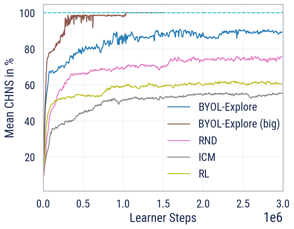
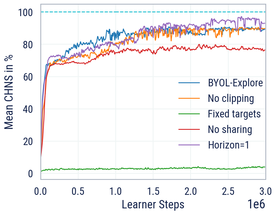
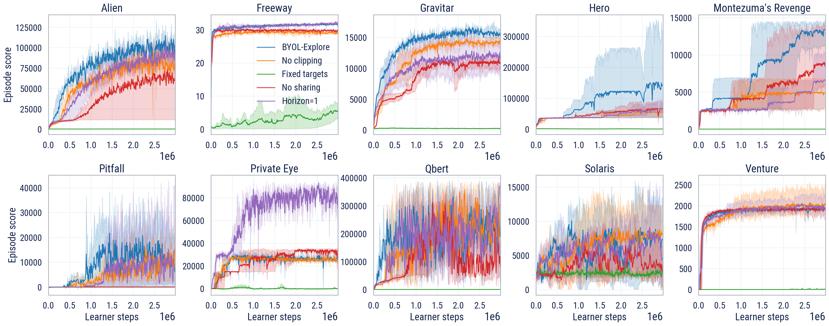
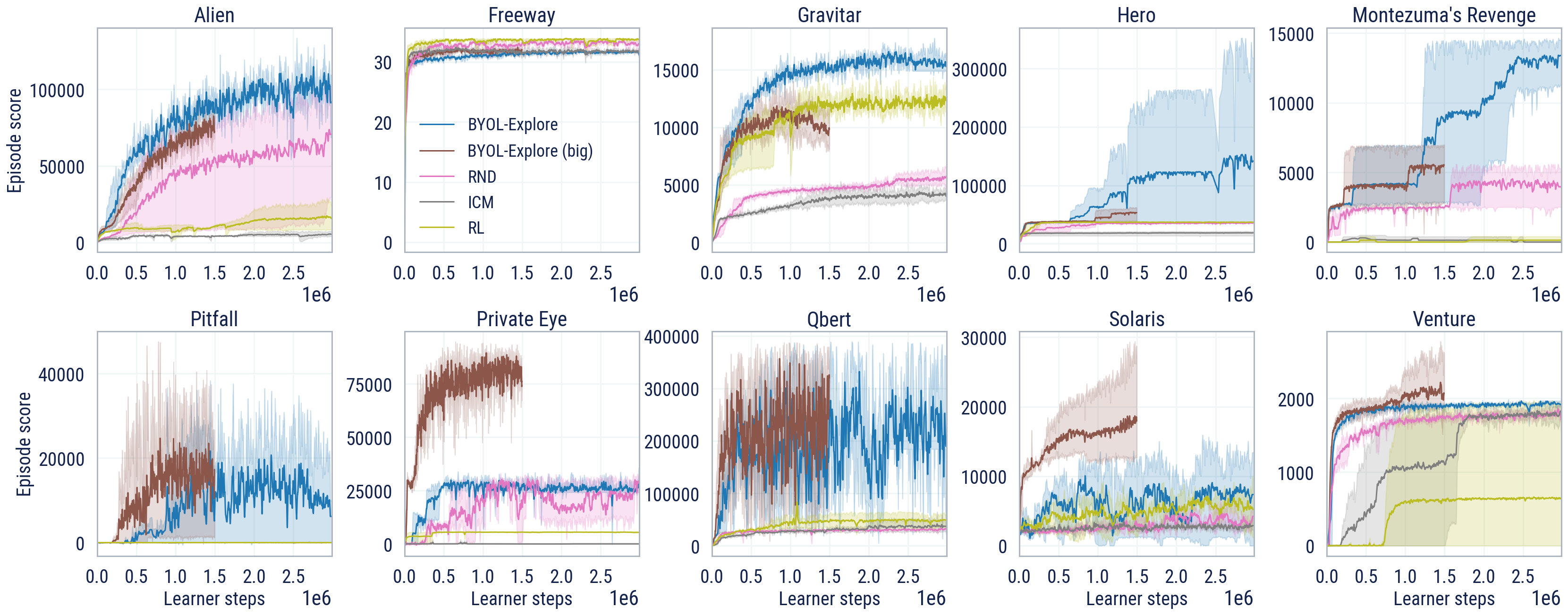
Fig. 3 (left) shows that BYOL-Explore is almost superhuman on the $10$-hardest exploration games and outperforms the different baselines of RND, ICM, and pure RL. Fig. 3 (right) compares BYOL-Explore against its ablations to gain finer insights into our method. The No clipping ablation performs comparably, showing that the prioritization of intrinsic rewards is not necessary on Atari tasks. Similarly, the Horizon=1 ablation performs slightly better, indicating that simply predicting one-step latents is sufficient to explore efficiently on the fully-observable Atari tasks. The Fixed Targets ablation performs much worse, showing that our approach of predicting learned targets (rather than fixed random projections) is vital for good performance. It is also worth noting that all the ablations except Fixed Targets outperform all of our baselines, demonstrating the robustness of our approach.

Finally, because the Horizon=1 ablation was close to superhuman on Atari, we run the same configuration but double the length of the sequences on which we train from $64$ to $128$ (also doubling memory requirements while learning). For fair comparison, we train for only half the learner steps to keep total computation performed roughly equivalent. With this small adjustment, this agent (BYOL-Explore (big)) becomes superhuman on all of the $10$-hardest exploration games.

Figure 4: Number of rooms visited in Montezuma’s Revenge during training in the self-supervised regime over $3$ seeds.

Purely intrinsic exploration.

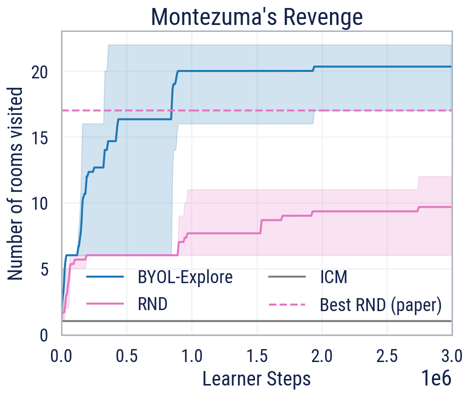
To test how BYOL-Explore behaves when only given intrinsic rewards without any extrinsic signal, we test on the well-known Montezuma’s Revenge game by setting $\lambda=0$. We measure exploratory behavior in terms of the number of different rooms of the dungeon the agent is able to explore over its lifetime. Note that accessing later rooms requires navigating complex dynamics such as collecting keys to open doors, avoiding enemies, and carefully traversing rooms filled with traps such as timed lasers. Figure 4 shows how much room coverage is achieved during training when no extrinsic reward is used, showing that BYOL-Explore explores further than the best result reported by RND [9]. Importantly, we use the episodic setting for intrinsic rewards whereas the published RND results considers the non-episodic setting for intrinsic rewards — facilitating exploration as the agent is less risk-averse. Therefore, our setting could be considered even more challenging. Our agent explores more than $20$ rooms on average versus $17$ with best published RND results. As expected in the episodic setting, our RND re-implementation visits even fewer rooms. However, we can reproduce the published RND results in the episodic setting when using recurrent policies.

Further results.

More fine-grained results are reported in App D.1. We report, in Fig.10 and in Fig.11, the agent scores learning curves for each game. Tab. 1 and Tab. 2 have agent score at the end of training. Finally, Tab. 3 and Tab. 4 show the mean CHNS and different statistics (mean and percentiles) of the HNS across the selected games.

An interesting finding from examining the HNS is that clipping and longer-horizon predictions are critical for very high scores on some games such as Montezuma’s Revenge or Hero. BYOL-Explore has a median HNS of $331.98$ compared to the No-clipping ablation and the Horizon=1 which have a median HNS of only $181.39$ and $199.80$ respectively. Therefore, while clipping is not necessary to get to human-level performance, it is still crucial to achieve top performance.

We also provide further results regarding the pure exploration setting on all 10 games in App. D.2.

4.3 DM-HARD-8 Results

In these experiments, we set the target EMA rate $\alpha=0.99$ and open-loop horizon $K=10$. We use $\lambda=0.01$ to combine the intrinsic and extrinsic rewards.

In contrast to prior work [22], we perform experiments in the more challenging multi-task regime, training a single agent to solve all eight tasks. At the beginning of each episode, a task is drawn uniformly at random from the suite.

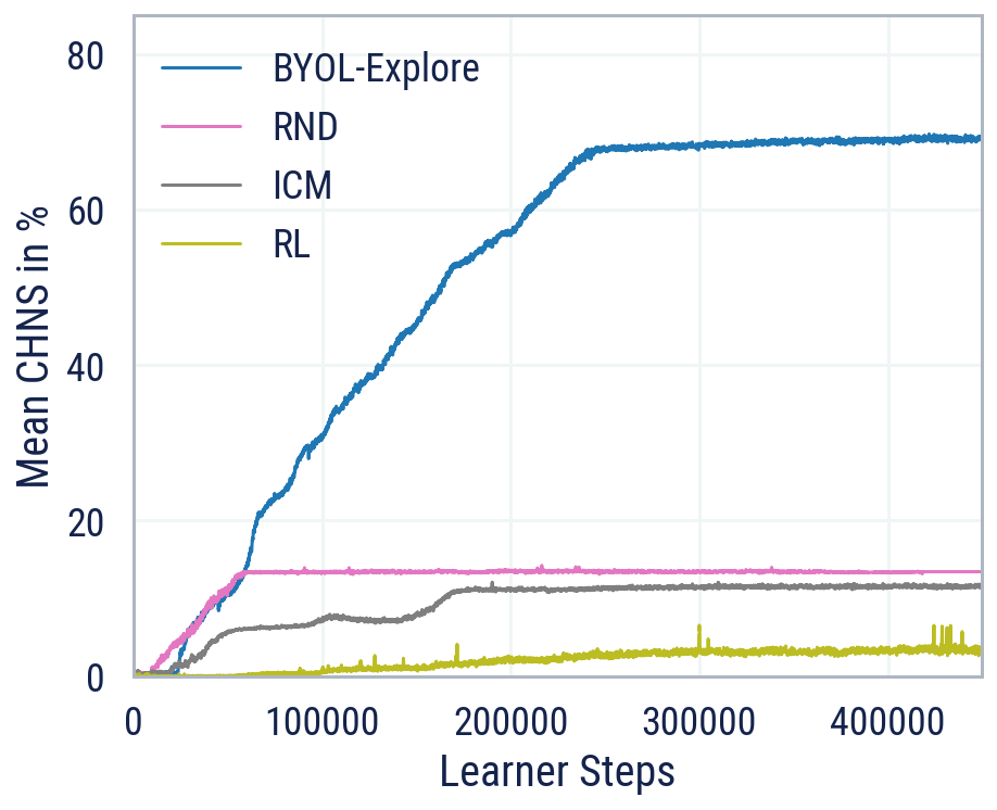
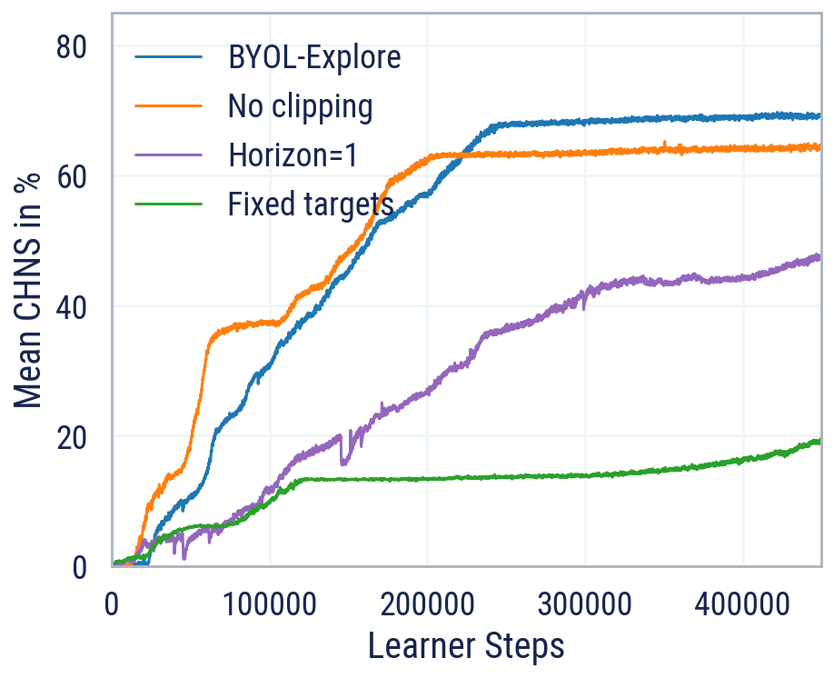
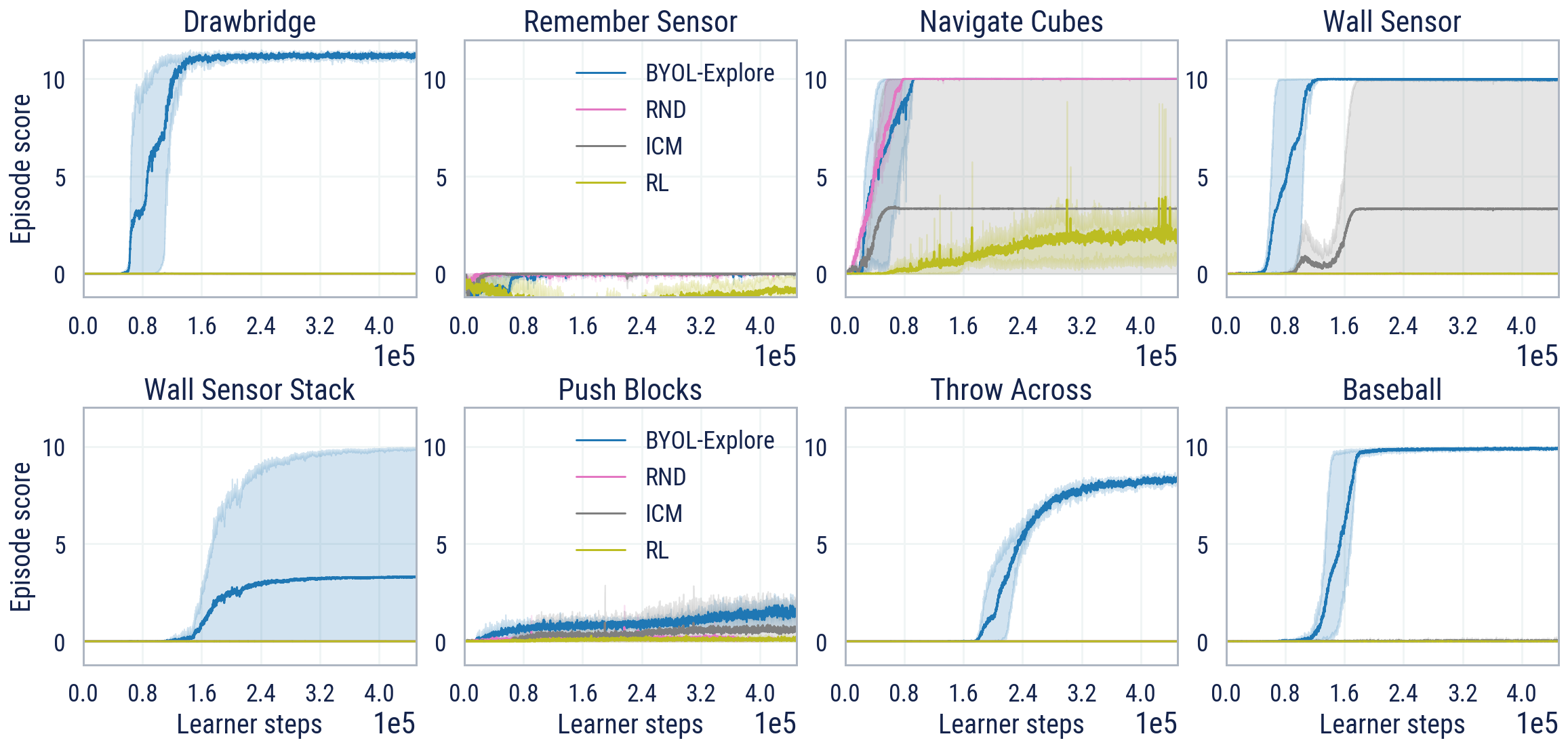
In Fig. 5 (left) we report the mean $\texttt{CHNS}(t)$ across the tasks, averaged over 3 seeds. We see that BYOL-Explore outperforms the baselines of RND, ICM, and pure RL by a large margin. Fig. 5 (right) compares the performance of BYOL-Explore to its various ablations. Note that the No-clipping ablation performs similarly to BYOL-Explore in terms of CHNS. However, unlike the fully-observable Atari tasks, the Horizon=1 ablation learns considerably slower and achieves lower final performance (see also our extended ablations on the horizon length in Fig. 14 in App. D.3). We note once again that the BYOL-Explore bootstrapping mechanism for learning representations is essential, as confirmed by the poor (but non-zero) performance of the Fixed-targets ablation. Due to computational limitations, we did not run the No Sharing ablation, as using separate networks requires twice the memory.

Figure 5: Mean $\texttt{CHNS}(t)$ score across the tasks in the DM-HARD-8 suite. Left: BYOL-Explore against baselines: ICM, RND and Pure RL. Right: BYOL-Explore against various ablations.

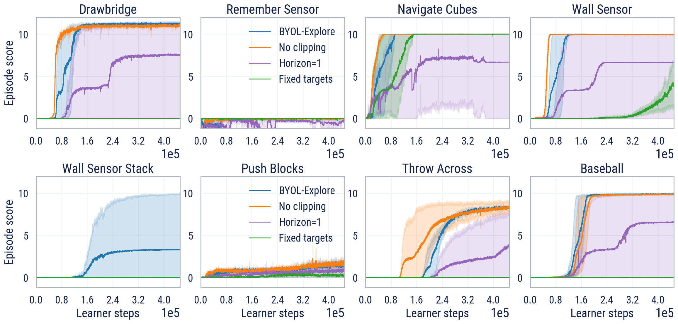
We now analyze our method more closely by examining per-task performance. The full learning curves for each task can be found in Fig. 6 for BYOL-Explore and the main baselines and in Appendix D.3 (see Fig. 13) for the various ablations. First, we take note that other curiosity-driven methods (ICM and RND) cannot get any positive score on the majority of the DM-HARD-8 tasks, even with additional hyperparameter tuning and reward prioritizing (see Fig. 16 and Fig. 17 in App. D.3).

In contrast, we see that BYOL-Explore achieves strong performance on five out of the eight hard exploration tasks. Importantly, BYOL-Explore achieves this without human demonstrations, which was not the case in prior work  [22]. BYOL-Explore even surpasses humans on $4$ tasks, namely Navigate cubes, Throw-across, Baseball, and Wall Sensors (see Tab. 9 in App. D.3 for details). Most impressively, BYOL-Explore can solve Throw-across, which is a challenging task even for a skilful human player and was not solvable in prior work without collecting additional successful human demonstrations  [22].

Interestingly, note that on the Navigate Cubes task, both RND and the Fixed-targets ablation achieve maximum performance alongside BYOL-Explore. We argue that this is because the prediction of random projections (either at the same step as done by RND or multi-step as done by BYOL-Explore) leads to the policy learned performing spatial, navigational exploration — this is the kind of behavior required to explore well on the Navigate Cubes task. In contrast, the other tasks require exploratory behavior involving interaction with objects and the use of tools, where both RND and the Fixed-targets ablation fail.

Finally, we observe that two games, namely Remember Sensor and Push Blocks, are particularly challenging, where all of our considered methods perform poorly. We hypothesize that this is due to the larger variety of procedurally generated objects spawned in these levels, and the need to remember previous cues in the environment leading to a hard credit assignment problem.

Figure 6: Agent’s score for each task in the DM-HARD-8 suite for BYOL-Explore against baselines. Shaded areas correspond to the minimum and maximum values across three seeds.

Purely intrinsic exploration.

Each of the DM-HARD-8 tasks has complex dynamics and object interactions, making it difficult to assess qualitatively the behavior of purely intrinsically motivated exploration. Nevertheless, for completeness, we provide results of BYOL-Explore trained only with intrinsic rewards in App. D.3, showing that it does achieve some positive signal on the Drawbridge and Wall Sensor tasks (see Fig. 18).

5 Conclusion

We showed that BYOL-Explore is a simple curiosity-driven exploration method that achieves excellent performance on hard exploration tasks with fairly deterministic dynamics. BYOL-Explore is a multi-step prediction error method at the latent level that relies on recent advances in self-supervised learning to train its representation as well as its world-model without any additional loss. In Atari, BYOL-Explore achieves superhuman performance on the $10$-hardest exploration games while being of much simpler design than other superhuman agents. Moreover, BYOL-Explore substantially outperforms previous exploration methods on DM-HARD-8 navigation and manipulation tasks in a $3$-D, multi-task, partially-observable and procedurally-generated environment. This shows the generality of our algorithm to handle either $2$-D or $3$-D, single or multi-task, fully or partially-observable environments.

In the future, we would like to improve performance in DM-HARD-8 and to demonstrate the generality of our method by extending it to other domains. In DM-HARD-8, we believe we can improve performance by scaling up the world model and finding better ways to trade off exploration and exploitation. Beyond DM-HARD-8, there are opportunities to tackle further challenges, most notably highly-stochastic and procedurally-generated environment dynamics such as NetHack [40].

Appendix A General BYOL-Explore Architecture

Figure 7: BYOL-Explore’s Neural Architecture.

The online network is composed of:

• Encoder: $f_{\theta}:\mathcal{O}\rightarrow\mathbb{R}^{N}$

• Close-loop RNN cell: $h^{c}_{\theta}:\mathbb{R}^{M}\times\mathbb{R}^{N}\times\mathcal{A}\rightarrow\mathbb{R}^{M}$

• Open-loop RNN cell: $h^{o}_{\theta}:\mathbb{R}^{M}\times\mathcal{A}\rightarrow\mathbb{R}^{M}$

• Predictor: $g_{\theta}:\mathbb{R}^{M}\rightarrow\mathbb{R}^{N}$

The target network is composed of:

• EMA encoder: $f_{\phi}:\mathcal{O}\rightarrow\mathbb{R}^{N}$

A.1 Detailed BYOL-Explore architecture for Atari

In Atari, the size of the observation-representation $N=512$ and the size of the history-representation $M=256$.

• Encoder: $f_{\theta}:\mathcal{O}\rightarrow\mathbb{R}^{N}$: The encoder is instantiated as a Deep ResNet [30] stack. The greyscale image observation is passed through a stack of 3 units, each comprised of a $3\times 3$ convolutional layer, a $3\times 3$ maxpool layer, and 2 residual blocks. The number of channels for the convolutional layer and the residual blocks are 16, 32, and 32 within each of the 3 units respectively. We use GroupNorm normalization [75] with one group at the end of each of the 3 units, and use ReLU activations everywhere. The output of the final residual block is flattened and projected using a single linear layer to an embedding of dimension $512$.

• Close-loop RNN cell: $h^{c}_{\theta}:\mathbb{R}^{M}\times\mathbb{R}^{N}\times\mathcal{A}\rightarrow\mathbb{R}^{M}$ is a simple Gated Recurrent Unit (GRU) [11]. We provide the past-action to the close-loop RNN cell, embedded into a representation of size $32$.

• Open-loop RNN cell: $h^{o}_{\theta}:\mathbb{R}^{M}\times\mathcal{A}\rightarrow\mathbb{R}^{M}$ is a simple Gated Recurrent Unit. We provide the past-action to the open-loop RNN cell, embedded into a representation of size $32$.

• Policy head $\pi_{\psi}:\mathbb{R}^{N}\rightarrow\mathbb{R}^{|\mathcal{A}|}$, value head $v_{\psi}:\mathbb{R}^{N}\rightarrow\mathbb{R}$, and BYOL-Explore predictor $g_{\theta}:\mathbb{R}^{M}\rightarrow\mathbb{R}^{N}$ are each a simple Multi-Layer Perceptron (MLP) with one hidden layer of size $256$. The outputs of the policy head are passed through a softmax layer to form the probabilities for each action to be taken.

A.2 Detailed BYOL-Explore architecture for DM-HARD-8

In DM-HARD-8, the size of the observation-representation $N=256$ and the size of the history-representation $M=512$.

• Encoder: $f_{\theta}:\mathcal{O}\rightarrow\mathbb{R}^{N}$: The encoder operates over RGB image observations at each timestep, and is implemented as a Deep ResNet [30] stack. The image is passed through a stack of 3 units, each comprised of a $3\times 3$ convolutional layer with stride 1, a $3\times 3$ maxpool layer with stride 2, and 2 residual blocks. We use ReLU activations everywhere. The output of this stack is flattened and passed through a linear layer of width 1024, followed by LayerNorm and ReLU layers, and finally a linear layer of width 256.

• Close-loop RNN cell: $h^{c}_{\theta}:\mathbb{R}^{M}\times\mathbb{R}^{N}\times\mathcal{A}\rightarrow\mathbb{R}^{M}$: The RNN cell operates over the output of the encoder $f_{\theta}$ in addition to some other observation signals per timestep, which we describe first. The observation contains (i) the force the agent’s hand is currently applying as a fraction of total grip strength, a single scalar between 0 and 1; (ii) a boolean indicating whether the hand is currently holding an object; (iii) the distance of the agent hand from the main body; (iv) the last action taken by the agent; each of these are embedded using a linear projection to 20 dimensions followed by a ReLU. (v) the previous reward obtained by the agent, passed by a signed hyperbolic transformation; (vi) a text instruction specific to the task currently being solved, with each word embedded into 20 dimensions and processed sequentially by an LSTM to an embedding of size 64. All of these quantities, along with the output of $f_{\theta}$, are concatenated and passed through a linear layer to an embedding of size 512. An LSTM with embedding size 512 processes each of these observation representations sequentially to form the recurrent history-representation.

• Open-loop RNN cell: $h^{o}_{\theta}:\mathbb{R}^{M}\times\mathcal{A}\rightarrow\mathbb{R}^{M}$: This is implemented as an LSTM. We discretize the action into 76 bins and provide them as one-hot representations of the action for the partial history unroll.

• Policy head $\pi_{\psi}:\mathbb{R}^{N}\rightarrow\mathbb{R}^{|\mathcal{A}|}$, value head $v_{\psi}:\mathbb{R}^{N}\rightarrow\mathbb{R}$, and BYOL-Explore predictor $g_{\theta}:\mathbb{R}^{M}\rightarrow\mathbb{R}^{N}$: These are each implemented as an MLP with hidden sizes of (512,), (512,), and (128, 256, 512,) respectively. The policy network uses different linear projections of the shared hidden layer to compute components of the policy over different parts of the action space. The action space has a mix of both discrete (modeled using a softmax layer of logits computed as linear projection of the hidden layer) as well as continuous (modeled as Gaussian distributions over each dimension with the mean and variance modeled using a linear projection of the hidden layer) actions, described in detail in prior works [22].

A.3 Detailes of Reward Normalization Mechanism

We use a similar reward normalization scheme as in RND [9] and normalize the raw rewards $((\ell^{\,j}_{t})_{t=0}^{T-2})_{j=0}^{B-1}$ by an EMA estimate of their standard deviation.

More precisely, we first set the EMA mean to $\overline{r}=0$, the EMA mean of squares to $\overline{r^{2}}=0$ and the counter to $c=1$. Then, for the $c$-th batch of raw rewards $((\ell^{\,j}_{t})_{t=0}^{T-2})_{j=0}^{B-1}$, we compute the batch mean $\overline{r_{c}}$ and the batch mean of squares $\overline{r^{2}_{c}}$ :

$$\overline{r_{c}}=\frac{1}{B(T-1)}\sum_{j=0}^{B-1}\sum_{t=0}^{T-2}\ell^{\,i}_{t},\qquad\overline{r^{2}_{c}}=\frac{1}{B(T-1)}\sum_{j=0}^{B-1}\sum_{t=0}^{T-2}(\ell^{\,i}_{t})^{2}.\\$$

We then update $\overline{r}$, $\overline{r^{2}}$ and $c$:

$$\overline{r}\leftarrow\alpha_{r}\overline{r}+(1-\alpha_{r})\overline{r_{c}},\qquad\overline{r^{2}}\leftarrow\alpha_{r}\overline{r^{2}}+(1-\alpha_{r})\overline{r^{2}_{c}},\qquad c\leftarrow c+1,$$

where $\alpha_{r}=0.99$. We compute the adjusted EMA mean $\mu_{r}$, the adjusted EMA mean of squares $\mu_{r^{2}}$:

$$\mu_{r}=\frac{\overline{r}}{1-\alpha_{r}^{c}}\mathbin{\raisebox{2.15277pt}{,}}\qquad\mu_{r^{2}}=\frac{\overline{r^{2}}}{1-\alpha_{r}^{c}}\cdot$$

Finally the EMA estimation of the standard deviation is $\sigma_{r}=\sqrt{\max(\mu_{r^{2}}-\mu_{r}^{2},0)+\varepsilon}$, where $\varepsilon=10^{-8}$ is a small numerical regularization. The normalized rewards are $\ell^{\,j}_{t}/\sigma_{r}$.

Appendix B Baselines

Random Network Distillation (RND) [9]

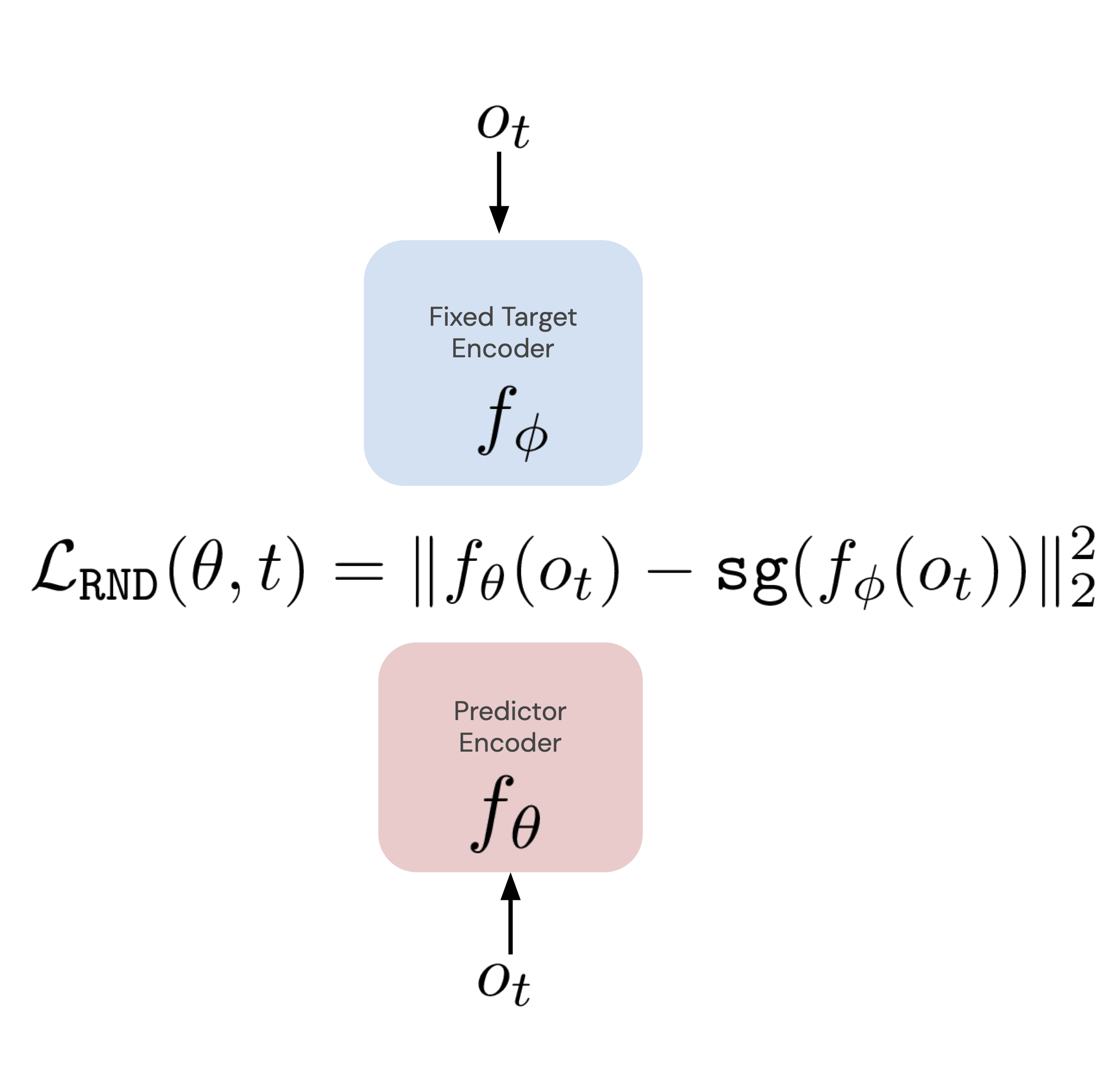
is a simple exploration method that consists in training an encoder such that its outputs fit the outputs of another fixed and randomly initialized encoder and using the training loss as an intrinsic reward to be optimized by an RL algorithm. More precisely, let $N\in\mathbb{N}^{*}$ be the embedding size and let us note $f_{\theta}:\mathcal{O}\rightarrow\mathbb{R}^{N}$ the encoder, also called predictor network, with trainable weights $\theta$ and $f_{\phi}:\mathcal{O}\rightarrow\mathbb{R}^{N}$ the fixed and randomly initialized encoder, also called target network, with fixed weights $\phi$. In addition, let us suppose that we have a batch of trajectories $\mathopen{}\mathclose{{}\left((o^{j}_{t},a^{j}_{t})_{t=0}^{T-1}}\right)_{j=0}^{B-1}$ collected by our RL agent, then the loss $\mathcal{L}_{\texttt{RND}}(\theta)$ to minimize w.r.t. the online network parameters is defined as:

$$\mathcal{L}_{\texttt{RND}}(\theta,j,t)=\|f_{\theta}(o^{j}_{t})-\texttt{sg}(f_{\phi}(o^{j}_{t}))\|_{2}^{2},\quad\mathcal{L}_{\texttt{RND}}(\theta)=\frac{1}{BT}\sum_{j=0}^{B-1}\sum_{t=0}^{T-1}\mathcal{L}_{\texttt{RND}}(\theta,j,t),$$

and the unnormalized reward associated to the transition $(o^{j}_{t},a^{j}_{t},o^{j}_{t+1})$ is defined as $\ell^{\,j}_{t}=\mathcal{L}_{\texttt{RND}}(\theta,j,t+1)$ where $0\leq t\leq T-2$. To obtained the final intrinsic rewards, we just normalize them to be as close as possible to the original RND implementation:$r^{j}_{i,t}=\frac{\ell^{\,i}_{t}}{\sigma_{r}}$.

Figure 8: RND’s Neural Architecture.

Intrinsic Curiosity Module (ICM) [50]

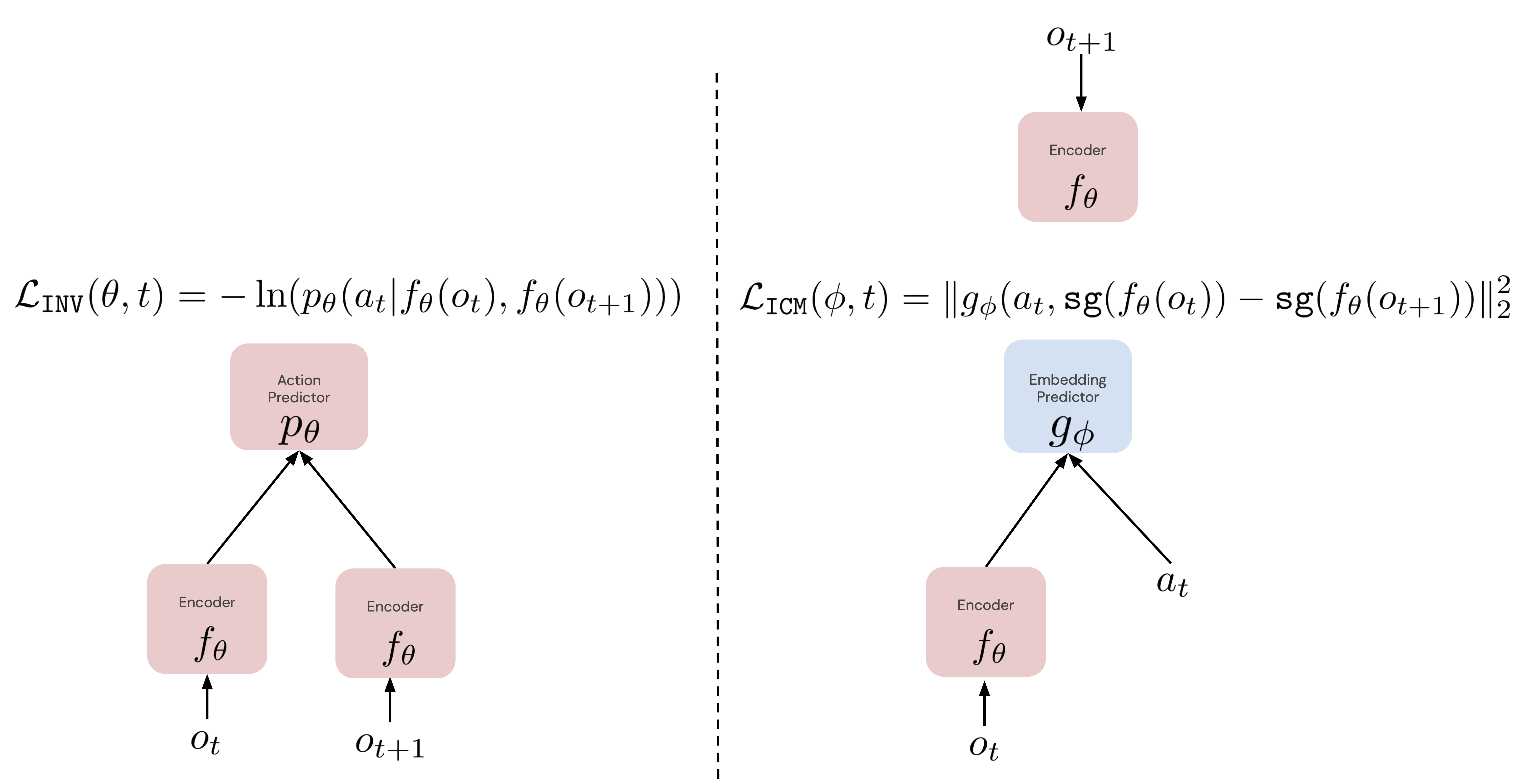
is a one-step prediction error method at the latent level. It consists in training an encoder $f_{\theta}:\mathcal{O}\rightarrow\mathbb{R}^{N}$ that outputs a representation that is robust to uncontrollable aspects of the environment and then use this representation as inputs of a one-step prediction error model $g_{\phi}:\mathbb{R}^{N}\times\mathcal{A}\rightarrow\mathbb{R}^{N}$ which error is used as an intrinsic reward to be optimized by an RL algorithm. To build a representation robust to uncontrollable dynamics, the idea used in ICM is to train an inverse dynamics model $p_{\theta}:\mathbb{R}^{N}\times\mathcal{R}^{N}\rightarrow\mathcal{A}$ that predicts the distribution of actions that led to the transition between two consecutive representations $f_{\theta}(o_{t}),f_{\theta}(o_{t+1})$. More precisely, let us suppose that we have a batch of trajectories $\mathopen{}\mathclose{{}\left((o^{j}_{t},a^{j}_{t})_{t=0}^{T-1}}\right)_{j=0}^{B-1}$ collected by our RL agent, then the loss $\mathcal{L}_{\texttt{INV}}(\theta)$ to minimize in order to train our encoder and inverse dynamcis model is:

$$\mathcal{L}_{\texttt{INV}}(\theta,j,t)=-\ln\mathopen{}\mathclose{{}\left(p_{\theta}(a^{j}_{t}|f_{\theta}(o^{j}_{t}),f_{\theta}(o^{j}_{t+1}))}\right),\quad\mathcal{L}_{\texttt{INV}}(\theta)=\frac{1}{B(T-1)}\sum_{j=0}^{B-1}\sum_{t=0}^{T-2}\mathcal{L}_{\texttt{INV}}(\theta,j,t),$$

which is a simple cross-entropy loss. Simultaneously, ICM also trains the one step prediction error model by minimizing the following one-step prediction loss:

$$\mathcal{L}_{\texttt{ICM}}(\phi,j,t)=\|g_{\phi}(f_{\theta}(o^{j}_{t}),a^{j}_{t})-\texttt{sg}(f_{\theta}(o^{j}_{t+1}))\|_{2}^{2},\quad\mathcal{L}_{\texttt{ICM}}(\phi)=\frac{1}{B(T-1)}\sum_{j=0}^{B-1}\sum_{t=0}^{T-2}\mathcal{L}_{\texttt{ICM}}(\theta,j,t),$$

and the unnormalized reward associated to the transition $(o^{j}_{t},a^{j}_{t},o^{j}_{t+1})$ is defined as $\ell^{\,j}_{t}=\mathcal{L}_{\texttt{ICM}}(\theta,j,t)$ where $0\leq t\leq T-2$. To obtained the final intrinsic rewards, we just normalize them :$r^{j}_{i,t}=\frac{\ell^{\,j}_{t}}{\sigma_{r}}$.

Figure 9: ICM’s Neural Architecture.

Appendix C Hyperparameter Settings

Atari Settings

We perform PopArt-style [32] reward normalization with a step size of 0.01, and after normalizing rescale the rewards by $1-\gamma$. We also similarly use PopArt normalization on the output of the value network.

We use a discount factor of $\gamma=0.999$. To train the value function, we use VTrace without offpolicy corrections to define TD targets for MSE loss with a loss weight of 0.5. We add an entropy loss with a loss weight of 0.001. The VMPO parameters $\eta_{init}$ and $\alpha_{init}$ are initialized to 0.5. $\varepsilon_{\eta}$ and $\varepsilon_{\alpha}$ are set to 0.01 and 0.005 respectively. We scale the BYOL loss by a factor of 5.0 when combining losses. The VMPO top-k parameter is set to 0.5. We use the Adam optimizer with learning rate $10^{-4}$ and $b_{1}=0.9$. The target network for VMPO is updated every 10 learner steps.

We use a batch size of 32 and a sequence length of 128; and a distributed learning setup using 4 TPUv2 for learning and 400 CPU actors for generating data via another inference server using 4 TPUv2 to evaluate the policy, similar to Agent57 [4].

DM-HARD-8 Settings

We perform separately PopArt for both the intrinsic and extrinsic rewards, on the multi-task suite of environments. We use a step size of $10^{-5}$ for extrinsic popart and 0.01 for intrinsic popart.

We use a discount factor of $\gamma=0.99$. To train the value function, we use VTrace without offpolicy corrections to define TD targets for MSE loss with a loss weight of 0.5. We do not add an entropy loss term. We scale the BYOL loss by a factor of 1.0 when combining losses. The VMPO top-k parameter is set to 0.5. The VMPO temperature parameters $\eta_{init}$ and $\varepsilon_{\eta}$ are set to 1.0 and 0.1 respectively. For the discrete components of the action, the VMPO KL constraint parameters $\alpha_{init\_categorical}$ and $\varepsilon_{\alpha\_categorical}$ are set to 5.0 and 0.0016 respectively. For the continuous Gaussian actions, we found it important to apply the VMPO contraints separately to the mean and covariance of the distributions, per action dimension. Thus for the mean, $\alpha_{init\_mean}$ and $\varepsilon_{\alpha\_mean}$ are 1.0 and 0.001 respectively; for the covariance, $\alpha_{init\_covariance}$ and $\varepsilon_{\alpha\_covariance}$ are 1.0 and 0.0001 respectively.

We use the Adam optimizer with learning rate $10^{-4}$ and $b_{1}=0.0$. The target network for VMPO is updated every 10 learner steps.

We use a batch size of 48 and a sequence length of 80; and use a distributed learning setup consisting of 8 TPUv3 divided into 6 for learning and 2 for acting similar to the Sebulba [31] framework.

Appendix D Further Experimental Results

D.1 Atari: Detailed results when mixing intrinsic and extrinsic rewards

For more detailed analysis of our agent performance, we provide detailed results broken down per-task and by showing statistics of the human normalized score across games other than simply the capped mean.

Table 1 and Figure 10 compare agent performance for BYOL-Explore and our various baselines considered, while Table 1 and Figure 11 compare BYOL-Explore to its various ablations.

Tables 3 and 4 show various finer-grained statistics of human normalized score averaged across all games, for BYOL-Explore compared to our baselines and its ablations, respectively.

Games	Average Human	BYOL-Explore	RND	ICM	RL	BYOL-Explore (big)
alien	7127.70	124524.02	74717.02	5664.83	18252.69	87754.33
freeway	29.60	32.12	33.74	32.61	33.97	32.62
gravitar	3351.40	17014.51	5885.23	4657.20	13541.10	12234.71
hero	30826.40	153124.29	36452.78	18753.97	37235.84	54139.73
montezuma revenge	4753.30	13518.18	4554.37	300.00	160.11	5615.36
pitfall	6463.70	25175.53	0.00	0.00	0.00	27555.12
private eye	69571.30	33130.85	33150.09	1419.49	5704.99	94589.47
qbert	13455.00	358269.62	34341.06	44294.63	91920.56	377349.65
solaris	12326.70	11060.24	5262.55	3924.22	8147.67	19277.35
venture	1187.50	1980.24	1879.68	1860.19	670.61	2250.12

Table 1: Maximum agent score obtained over training for BYOL-Explore and the baselines for 10 hard-exploration Atari games, averaged over 10 episodes and 3 seeds.

Games	Average Human	BYOL-Explore	No clipping	Fixed targets	No sharing	Horizon=1
alien	7127.70	124524.02	99570.34	411.63	75876.95	105384.32
freeway	29.60	32.12	30.13	6.09	30.63	32.73
gravitar	3351.40	17014.51	14949.85	401.79	12026.79	13621.41
hero	30826.40	153124.29	55897.06	1963.10	67555.39	67954.99
montezuma revenge	4753.30	13518.18	5093.32	8.52	9090.71	6701.77
pitfall	6463.70	25175.53	19427.77	-3.55	0.00	17363.46
private eye	69571.30	33130.85	31048.56	1706.72	36183.65	95359.23
qbert	13455.00	358269.62	370719.60	565.59	338709.48	368757.50
solaris	12326.70	11060.24	10380.94	3772.82	7105.23	9585.28
venture	1187.50	1980.24	2121.38	31.12	1977.89	2078.24

Table 2: Maximum agent score obtained over training for BYOL-Explore and the ablations for 10 hard-exploration Atari games, averaged over 10 episodes and 3 seeds.

Statistics	BYOL-Explore	RND	ICM	RL	BYOL-Explore (big)
Mean CHNS	93.62	78.32	57.43	63.38	100.00
Number of superhuman games	8	6	4	5	10
Mean HNS	661.14	209.08	91.42	174.22	579.57
Median HNS	331.98	116.44	69.14	88.55	183.86
40% Percentile HNS	237.34	106.72	45.39	59.98	172.01
30% Percentile HNS	149.28	81.36	18.86	41.98	154.66
20% Percentile HNS	104.52	45.37	5.73	7.22	132.41
10% Percentile HNS	84.48	33.02	3.29	3.42	117.34
5% Percentile HNS	66.04	18.22	2.65	3.39	113.78

Table 3: Statistics of human-normalized score (HNS) and Clipped HNS (CHNS) over the $10$-hardest exploration games for BYOL-Explore and baselines, averaged over 10 episodes and 3 seeds.

Statistics	BYOL-Explore	No clipping	Fixed targets	No sharing	Horizon=1
Mean CHNS	93.62	92.71	6.81	80.83	97.53
Number of superhuman games	8	8	0	7	9
Mean HNS	661.14	568.52	6.81	480.94	584.68
Median HNS	331.98	181.39	3.08	178.90	199.80
40% Percentile HNS	237.34	150.05	2.88	141.32	161.40
30% Percentile HNS	149.28	105.54	2.65	88.30	139.82
20% Percentile HNS	104.52	97.92	2.58	52.73	131.78
10% Percentile HNS	84.48	78.67	2.19	47.14	107.05
5% Percentile HNS	66.04	61.64	1.19	25.28	91.17

Table 4: Statistics of human-normalized score (HNS) and Clipped HNS (CHNS) over the $10$-hardest exploration games for BYOL-Explore and its ablations, averaged over 10 episodes and 3 seeds.

Figure 10: Learning curves in terms of agent score for BYOL-Explore and baselines for Atari, averaged over 10 episodes and 3 seeds.

Figure 11: Learning curves in terms of agent score for BYOL-Explore and its ablations for Atari, averaged over 10 episodes and 3 seeds.

D.2 Atari: Detailed results for the pure exploration regime

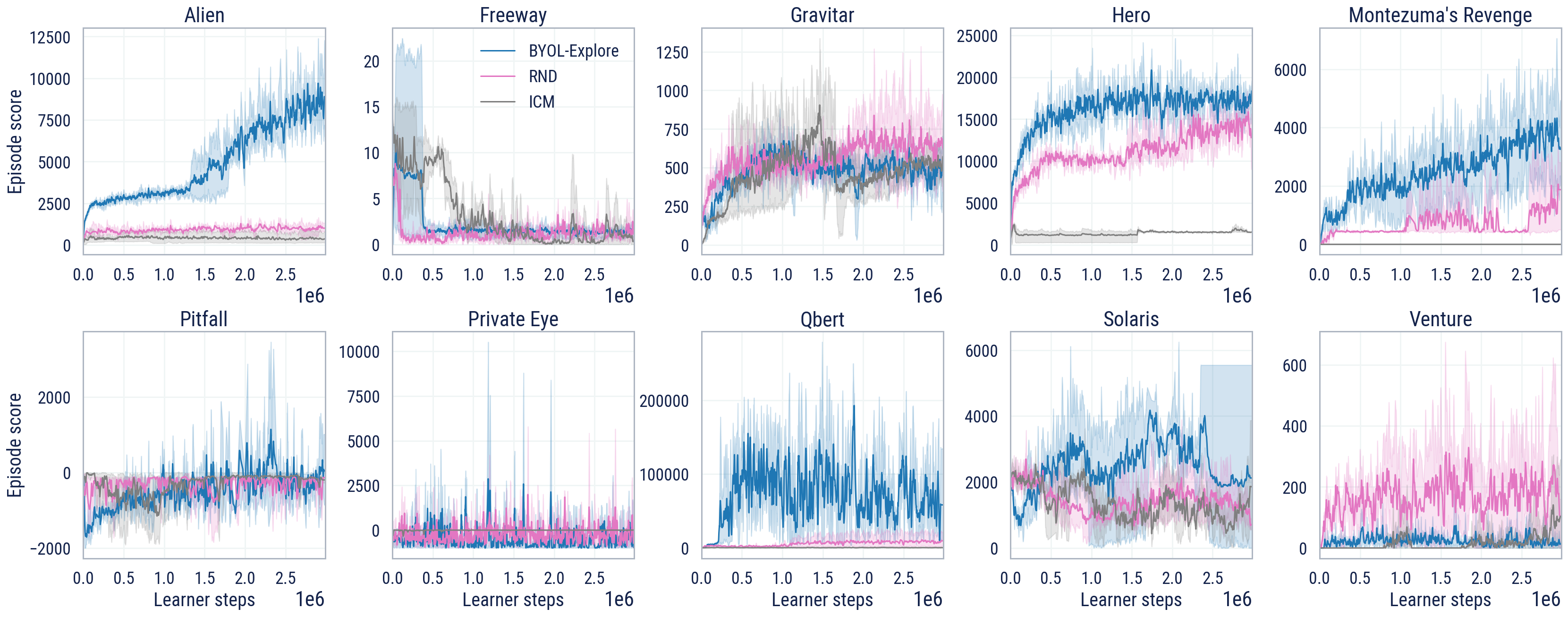
To further evaluate BYOL-Explore as an approach for curiousity-driven exploration, we examine the performance of an agent trained only using intrinsic rewards, without ever using the extrinsic reward signal. In the task Montezuma’s Revenge, Figure 4 measures the quality of exploraton in terms of the number of different rooms of the dungeon the agent is able to explore without using extrinsic rewards. However, computing this requires access to privileged information and detailed understanding of the environment design, and this kind of analysis is not easily adapted to a wider range of diverse games. Thus, as a proxy for engaging in interesting behavior in the environment, we measure exploratory behavior in terms of the extrinsic reward the agent obtains. As obtaining large amounts of extrinsic reward requires visiting many different regions of the state space and efficient exploration is highly correlated with this behavior, this is a reasonable measure for evaluating the quality of our agents. However, we stress again that though we measure performance in terms of the extrinsic reward, the agent is never given access to these reward signals while training.

Table 5 shows a summary of performance in each of the 10 hard-exploration games we consider, while Figure 12 shows performance through training.

Notice that BYOL-Explore is the only method to get positive rewards in Pitfall, showing that it can learn to effectively navigate the complex environment even without complex mechanisms such as Episodic Memory Modules used by prior works [4].

Games	Average Human	BYOL-Explore	RND	ICM
alien	7127.70	10964.95	1441.69	691.90
freeway	29.60	12.94	9.89	15.74
gravitar	3351.40	795.95	954.84	1040.45
hero	30826.40	22078.89	16964.23	2567.09
montezuma revenge	4753.30	5146.73	2305.65	2.68
pitfall	6463.70	1498.92	-83.55	-7.53
private eye	69571.30	5495.88	4309.31	469.09
qbert	13455.00	200081.13	12233.18	1062.49
solaris	12326.70	4298.20	2896.69	2851.86
venture	1187.50	101.25	399.53	157.99

Table 5: Maximum agent score obtained through training for BYOL-Explore and the baselines in the pure-exploration regime for Atari, averaged over 10 episodes and 3 seeds.

Figure 12: Learning curves in terms of agent score for BYOL-Explore and its ablations in the pure-exploration regime for Atari, averaged over 10 episodes and 3 seeds.

D.3 DM-HARD-8 Experiments

We similarly examine various statistics of agent performance on the DM-HARD-8 suite in terms of human-normalized score for BYOL-Explore versus our baselines (in Figure 6) and its ablations (in Figure 7).

Statistics	BYOL-Explore	RND	ICM	RL
Mean CHNS	69.87	14.36	12.42	7.10
Number of superhuman games	4	1	0	0
Mean HNS	83.92	17.89	12.42	7.10
Median HNS	101.21	0.21	3.35	0.21
40% Percentile HNS	81.74	0.09	0.83	0.15
30% Percentile HNS	43.98	0.02	0.24	0.11
20% Percentile HNS	28.71	0.00	0.13	0.05
10% Percentile HNS	17.20	0.00	0.08	0.01
5% Percentile HNS	11.45	0.00	0.04	0.01

Table 6: Statistics of human-normalized score (HNS) and Clipped HNS (CHNS) over the DM-HARD-8 suite for BYOL-Explore and baselines, averaged over 3 seeds.

Statistics	BYOL-Explore	No clipping	Fixed targets	Horizon=1
Mean CHNS	69.87	65.45	19.85	50.60
Number of superhuman games	4	4	1	1
Mean HNS	83.92	79.50	23.38	51.32
Median HNS	101.21	100.44	2.91	65.03
40% Percentile HNS	81.74	78.15	0.10	52.30
30% Percentile HNS	43.98	33.18	0.09	17.50
20% Percentile HNS	28.71	14.10	0.05	8.18
10% Percentile HNS	17.20	4.02	0.01	3.79
5% Percentile HNS	11.45	2.10	0.01	2.04

Table 7: Statistics of human-normalized score (HNS) and Clipped HNS (CHNS) over the DM-HARD-8 suite for BYOL-Explore and its ablations, averaged over 3 seeds.

Next, we examine per-task performance across each task within the DM-HARD-8 suite for BYOL-Explore compared with our baselines (in Table 8 and Figure 6), and compared with our main ablations (in Table 9).

Games	Average Human	BYOL-Explore	RND	ICM	RL
Drawbridge	12.30	11.38	0.00	0.02	0.00
Remember Sensor	7.60	0.00	0.00	0.00	-0.29
Navigate Cubes	7.80	10.00	10.00	3.46	3.95
Wall Sensor	9.10	10.00	0.03	3.33	0.02
Wall Sensor Stack	8.60	3.32	0.00	0.01	0.01
Push Blocks	8.40	1.86	0.73	0.96	0.30
Throw Across	5.70	8.46	0.00	0.00	0.00
Baseball	7.90	9.94	0.01	0.08	0.01

Table 8: Maximum agent score obtained through training for BYOL-Explore and our baselines for the various tasks in the DM-HARD-8 suite, averaged over 3 seeds.

Games	Average Human	BYOL-Explore	No clipping	Fixed targets	Horizon=1
Drawbridge	12.30	11.38	11.19	0.00	7.66
Remember Sensor	7.60	0.00	-0.00	0.00	-0.03
Navigate Cubes	7.80	10.00	10.00	10.00	8.25
Wall Sensor	9.10	10.00	10.00	4.24	6.66
Wall Sensor Stack	8.60	3.32	0.02	0.01	0.02
Push Blocks	8.40	1.86	2.25	0.52	1.05
Throw Across	5.70	8.46	8.48	0.00	3.87
Baseball	7.90	9.94	9.91	0.01	6.59

Table 9: Maximum agent score obtained through training for BYOL-Explore and its main ablations for the various tasks in the DM-HARD-8 suite, averaged over 3 seeds.

Figure 13: Learning curves in terms of agent score for BYOL-Explore and its main ablations for each task in the DM-HARD-8 suite, averaged over 3 seeds.

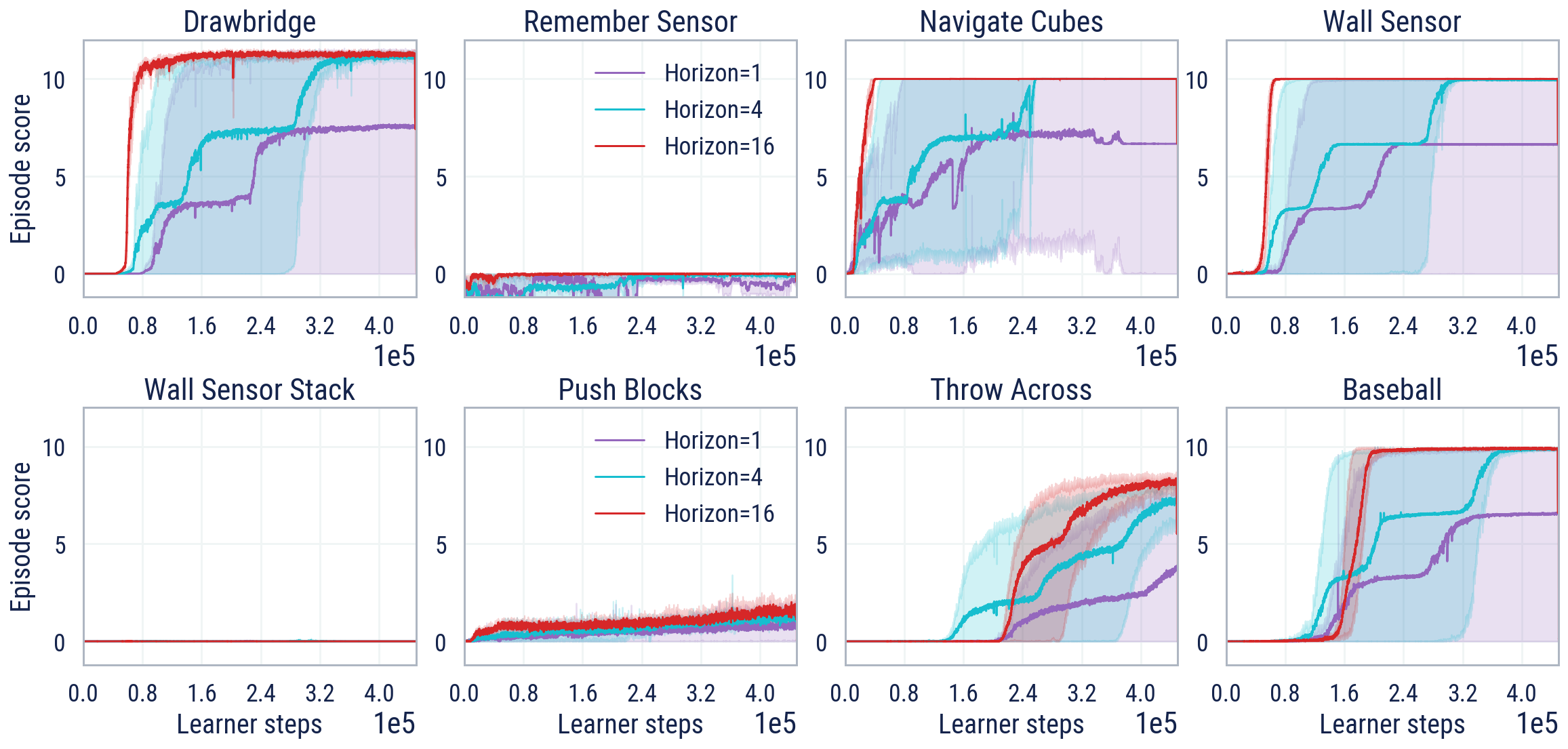
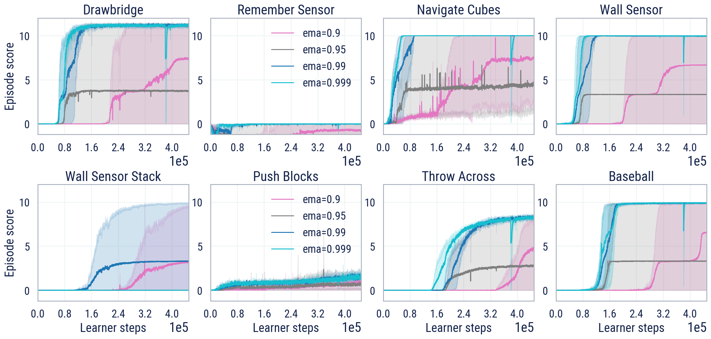
We also conduct further finer-grained ablations of BYOL-Explore parameters $K$ and $\alpha$. Recall that the main experiments used $K=10$ and $\alpha=0.99$. Figure 14 shows that increasing the open-loop horizon from $K=1$ to $16$ smoothly improves performance, showing the benefits of multi-step prediction of the future and the robustness of BYOL-Explore to this parameter. Figure 15 shows the effect of varying the EMA target parameter $\alpha$. We see that values BYOL-Explore is fairly robust to this hyperparameter, with the highest performance obtained by our base setting of $\alpha=0.99$.

Figure 14: Learning curves in terms of agent score for BYOL-Explore using varying lengths of open-loop horizon $K$ for multistep prediction, for each task in the DM-HARD-8 suite, averaged over 3 seeds.

Figure 15: Learning curves in terms of agent score for BYOL-Explore using varying values of EMA target parameter $\alpha$, for each task in the DM-HARD-8 suite, averaged over 3 seeds.

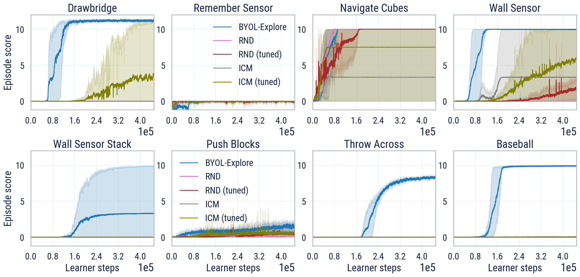
Next, we examine different improvements to our main baselines of RND and ICM. Note that for ease of comparison, the results reported for the baselines are using the same architectures and VMPO parameters as the BYOL-Explore settings. Nevertheless, for the sake of steelmanning our baselines, we separately tune both ICM and RND to maximize performance and report a comparison in Figure 16. We see that while performance can be improved slightly (at the expense of the tuned ICM and RND requiring more parameters), overall BYOL-Explore still outperforms across the board.

Figure 16: Learning curves in terms of agent score for BYOL-Explore compared against ICM and RND both using the same architecture/RL parameters and against baselines tuned separately, for each task in the DM-HARD-8 suite, averaged over 3 seeds.

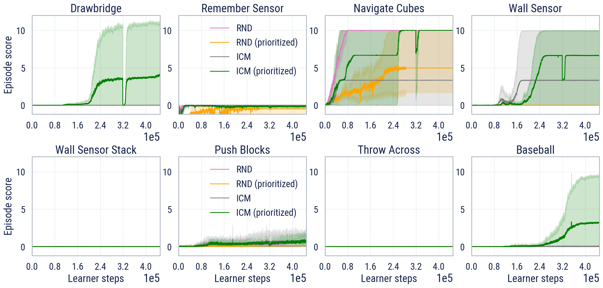
Aside from ablating the architectures and RL parameters, we also investigate whether our intrinsic reward prioritization mechanism via clipping can also improve the baselines of ICM and RND. Figure 17 shows that, again, while performance can be slightly improved, overall BYOL-Explore still outperforms baseline. Thus, multistep prediction of bootstrapped latents provides a qualitatively better intrinsic reward, aside from our contribution of a new reward normalization scheme.

Figure 17: Learning curves in terms of agent score for ICM and RND both with and without intrinsic reward prioritization via clipping, for each task in the DM-HARD-8 suite, averaged over 3 seeds.

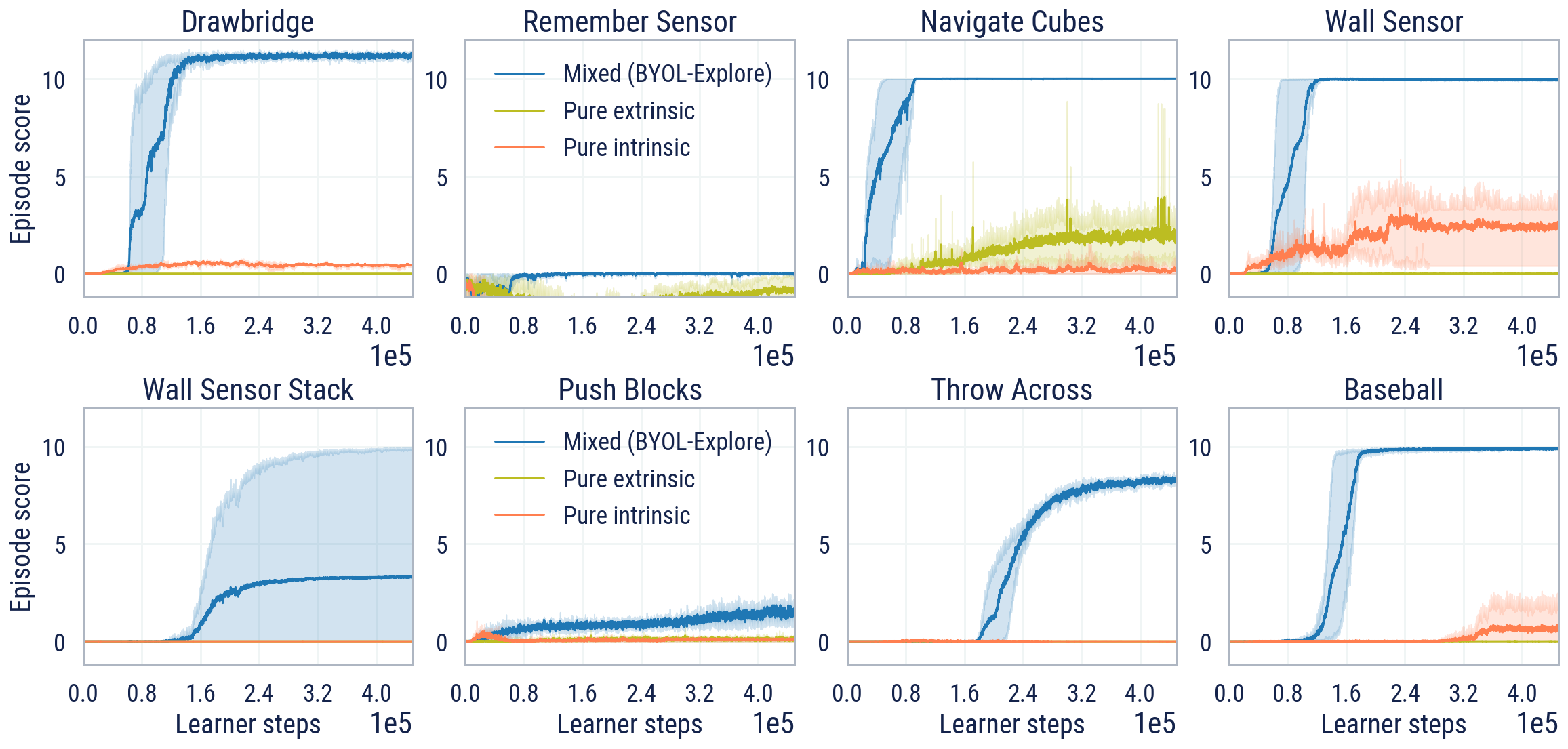
Similarly to Atari, in Figure 18, we also compare our mixed-intrinsic-extrinsic reward optimizing agent against agents optimizing purely intrinsic or extrinsic rewards. In the DM-HARD-8 domains, due to the much sparser reward than Atari, pure exploration in most tasks does not perform very well. However, remarkably it is still capable of achieving some positive signal on a handful of tasks, particularly Wall Sensor. Thus, purely maximizing intrinsic reward on DM-HARD-8 still results in meaningful exploration that leads the agent to display interesting behavior.

Figure 18: Learning curves in terms of agent score for for BYOL-Explore compared against both pure RL and pure-exploration settings, for each task in the DM-HARD-8 suite, averaged over 3 seeds.

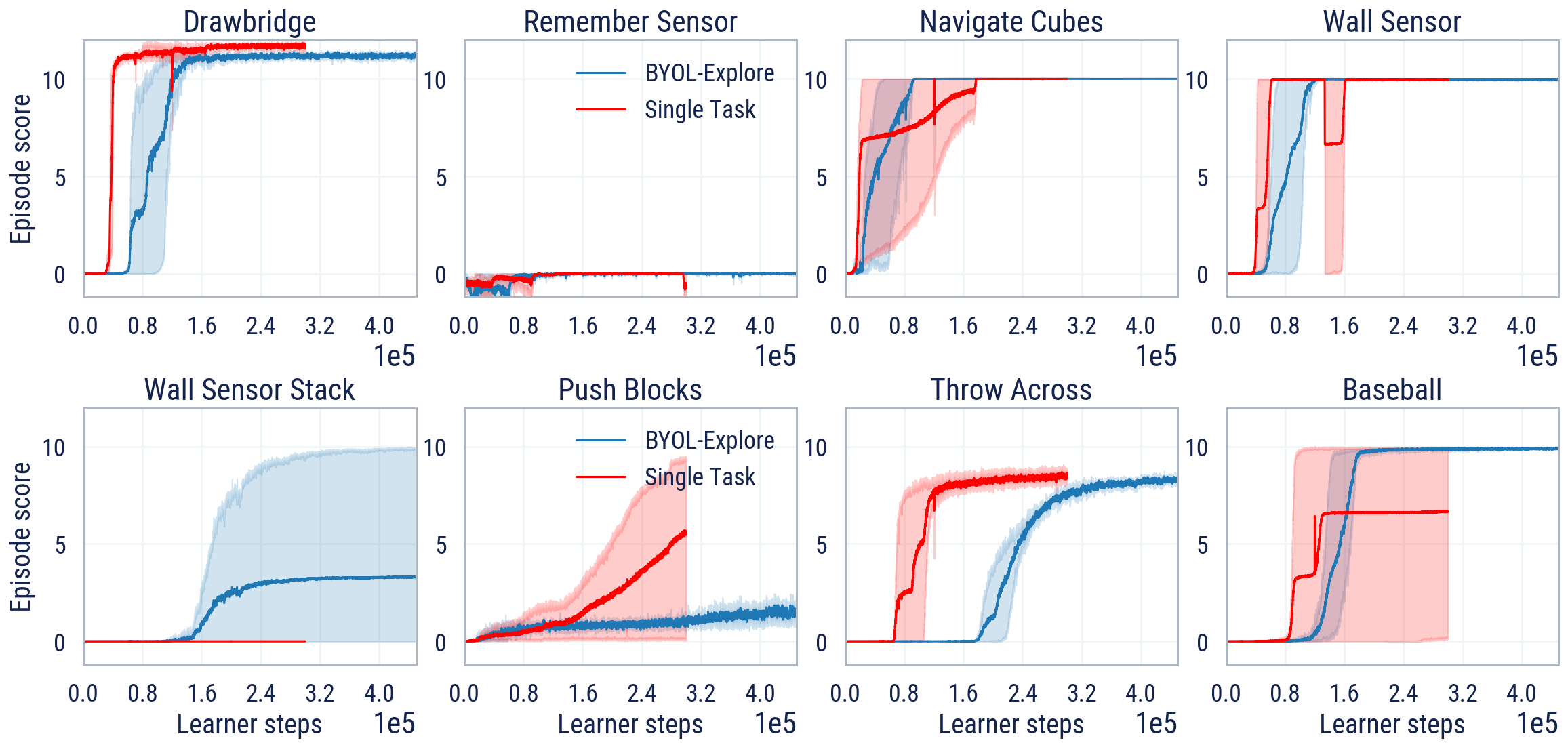
Finally, we note that we consider the considerably harder multi-task setting compared to the single-task setting chosen in prior work [22]. To ensure that the small amount of similarity between tasks does not induce any useful positive transfer and thus make the tasks easier when trained on multiple levels, for the sake of completeness we also report in Figure 19 the performance on single-task setting. As expected, performance is actually slightly higher in the single-task setting, thus showing that our strong multi-task results are not the result of any simplifying changes. Note also that the multi-task setting not only has to learn using a single set of parameters, it also receives $\frac{1}{8}$ of the training data per task in the DM-HARD-8 suite since we compare based on total experience across all tasks being equal.

Note that due to computational constraints we train the single-task version for $320000$ learner steps, but this is sufficient to demonstrate that single-task is not a harder setting than multi-task.

Figure 19: Learning curves in terms of agent score for for BYOL-Explore in the multi-task and single-task setting, for each task in the DM-HARD-8 suite, averaged over 3 seeds.

References

- [1] Marcin Andrychowicz, Filip Wolski, Alex Ray, Jonas Schneider, Rachel Fong, Peter Welinder, Bob McGrew, Josh Tobin, Pieter Abbeel, and Wojciech Zaremba. Hindsight experience replay. In Advances in neural information processing systems, pages 5048–5058, 2017.
- [2] Mohammad Gheshlaghi Azar, Bilal Piot, Bernardo Avila Pires, Jean-Bastien Grill, Florent Altché, and Rémi Munos. World discovery models. arXiv preprint arXiv:1902.07685, 2019.
- [3] Igor Babuschkin, Kate Baumli, Alison Bell, Surya Bhupatiraju, Jake Bruce, Peter Buchlovsky, David Budden, Trevor Cai, Aidan Clark, Ivo Danihelka, Claudio Fantacci, Jonathan Godwin, Chris Jones, Tom Hennigan, Matteo Hessel, Steven Kapturowski, Thomas Keck, Iurii Kemaev, Michael King, Lena Martens, Vladimir Mikulik, Tamara Norman, John Quan, George Papamakarios, Roman Ring, Francisco Ruiz, Alvaro Sanchez, Rosalia Schneider, Eren Sezener, Stephen Spencer, Srivatsan Srinivasan, Wojciech Stokowiec, and Fabio Viola. The DeepMind JAX Ecosystem. http://github.com/deepmind, 2020.
- [4] Adrià Puigdomènech Badia, Bilal Piot, Steven Kapturowski, Pablo Sprechmann, Alex Vitvitskyi, Zhaohan Daniel Guo, and Charles Blundell. Agent57: Outperforming the atari human benchmark. In International Conference on Machine Learning, pages 507–517. PMLR, 2020.
- [5] Adrià Puigdomènech Badia, Pablo Sprechmann, Alex Vitvitskyi, Daniel Guo, Bilal Piot, Steven Kapturowski, Olivier Tieleman, Martin Arjovsky, Alexander Pritzel, Andrew Bolt, and Charles Blundell. Never give up: Learning directed exploration strategies. In International Conference on Learning Representations, 2020.
- [6] Marc Bellemare, Sriram Srinivasan, Georg Ostrovski, Tom Schaul, David Saxton, and Remi Munos. Unifying count-based exploration and intrinsic motivation. In Advances in neural information processing systems, pages 1471–1479, 2016.
- [7] Marc G Bellemare, Yavar Naddaf, Joel Veness, and Michael Bowling. The arcade learning environment: An evaluation platform for general agents. Journal of Artificial Intelligence Research, 47:253–279, 2013.
- [8] Yuri Burda, Harri Edwards, Deepak Pathak, Amos Storkey, Trevor Darrell, and Alexei A Efros. Large-scale study of curiosity-driven learning. arXiv preprint arXiv:1808.04355, 2018.
- [9] Yuri Burda, Harrison Edwards, Amos Storkey, and Oleg Klimov. Exploration by random network distillation. In Seventh International Conference on Learning Representations, pages 1–17, 2019.
- [10] Xiaoyu Chen, Jiachen Hu, Lin F Yang, and Liwei Wang. Near-optimal reward-free exploration for linear mixture mdps with plug-in solver. arXiv preprint arXiv:2110.03244, 2021.
- [11] Kyunghyun Cho, Bart Van Merriënboer, Dzmitry Bahdanau, and Yoshua Bengio. On the properties of neural machine translation: Encoder-decoder approaches. arXiv preprint arXiv:1409.1259, 2014.
- [12] Junyoung Chung, Caglar Gulcehre, KyungHyun Cho, and Yoshua Bengio. Empirical evaluation of gated recurrent neural networks on sequence modeling. arXiv preprint arXiv:1412.3555, 2014.
- [13] Cédric Colas, Pierre Fournier, Mohamed Chetouani, Olivier Sigaud, and Pierre-Yves Oudeyer. Curious: intrinsically motivated modular multi-goal reinforcement learning. In International conference on machine learning, pages 1331–1340. PMLR, 2019.
- [14] Mayank Daswani, Peter Sunehag, and Marcus Hutter. Q-learning for history-based reinforcement learning. In Asian Conference on Machine Learning, pages 213–228. PMLR, 2013.
- [15] Adrien Ecoffet, Joost Huizinga, Joel Lehman, Kenneth O Stanley, and Jeff Clune. Go-explore: a new approach for hard-exploration problems. arXiv preprint arXiv:1901.10995, 2019.
- [16] Adrien Ecoffet, Joost Huizinga, Joel Lehman, Kenneth O Stanley, and Jeff Clune. First return, then explore. Nature, 590(7847):580–586, 2021.
- [17] Chelsea Finn, Ian Goodfellow, and Sergey Levine. Unsupervised learning for physical interaction through video prediction. Advances in neural information processing systems, 29, 2016.
- [18] Carlos Florensa, David Held, Xinyang Geng, and Pieter Abbeel. Automatic goal generation for reinforcement learning agents. In International Conference on Machine Learning, pages 1515–1528, 2018.
- [19] Meire Fortunato, Mohammad Gheshlaghi Azar, Bilal Piot, Jacob Menick, Ian Osband, Alex Graves, Vlad Mnih, Remi Munos, Demis Hassabis, Olivier Pietquin, et al. Noisy networks for exploration. arXiv preprint arXiv:1706.10295, 2017.
- [20] Karol Gregor, Danilo Jimenez Rezende, Frederic Besse, Yan Wu, Hamza Merzic, and Aaron van den Oord. Shaping belief states with generative environment models for rl. Advances in Neural Information Processing Systems, 32, 2019.
- [21] Jean-Bastien Grill, Florian Strub, Florent Altché, Corentin Tallec, Pierre Richemond, Elena Buchatskaya, Carl Doersch, Bernardo Avila Pires, Zhaohan Guo, Mohammad Gheshlaghi Azar, et al. Bootstrap your own latent-a new approach to self-supervised learning. Advances in Neural Information Processing Systems, 33:21271–21284, 2020.
- [22] Caglar Gulcehre, Tom Le Paine, Bobak Shahriari, Misha Denil, Matt Hoffman, Hubert Soyer, Richard Tanburn, Steven Kapturowski, Neil Rabinowitz, Duncan Williams, et al. Making efficient use of demonstrations to solve hard exploration problems. In International conference on learning representations, 2019.
- [23] Zhaohan Daniel Guo, Mohammad Gheshlagi Azar, Alaa Saade, Shantanu Thakoor, Bilal Piot, Bernardo Avila Pires, Michal Valko, Thomas Mesnard, Tor Lattimore, and Rémi Munos. Geometric entropic exploration. arXiv preprint arXiv:2101.02055, 2021.
- [24] Zhaohan Daniel Guo, Bernardo Avila Pires, Bilal Piot, Jean-Bastien Grill, Florent Altché, Rémi Munos, and Mohammad Gheshlaghi Azar. Bootstrap latent-predictive representations for multitask reinforcement learning. In International Conference on Machine Learning, pages 3875–3886. PMLR, 2020.
- [25] David Ha and Jürgen Schmidhuber. World models. arXiv preprint arXiv:1803.10122, 2018.
- [26] Danijar Hafner, Timothy Lillicrap, Jimmy Ba, and Mohammad Norouzi. Dream to control: Learning behaviors by latent imagination. arXiv preprint arXiv:1912.01603, 2019.
- [27] Danijar Hafner, Timothy Lillicrap, Ian Fischer, Ruben Villegas, David Ha, Honglak Lee, and James Davidson. Learning latent dynamics for planning from pixels. In International conference on machine learning, pages 2555–2565. PMLR, 2019.
- [28] Kristian Hartikainen, Xinyang Geng, Tuomas Haarnoja, and Sergey Levine. Dynamical distance learning for semi-supervised and unsupervised skill discovery. In International Conference on Learning Representations, 2020.
- [29] Elad Hazan, Sham Kakade, Karan Singh, and Abby Van Soest. Provably efficient maximum entropy exploration. In International Conference on Machine Learning, pages 2681–2691, 2019.
- [30] Kaiming He, Xiangyu Zhang, Shaoqing Ren, and Jian Sun. Deep residual learning for image recognition. In Proceedings of the IEEE conference on computer vision and pattern recognition, pages 770–778, 2016.
- [31] Matteo Hessel, Manuel Kroiss, Aidan Clark, Iurii Kemaev, John Quan, Thomas Keck, Fabio Viola, and Hado van Hasselt. Podracer architectures for scalable reinforcement learning. arXiv preprint arXiv:2104.06272, 2021.
- [32] Matteo Hessel, Hubert Soyer, Lasse Espeholt, Wojciech Czarnecki, Simon Schmitt, and Hado van Hasselt. Multi-task deep reinforcement learning with popart. In Proceedings of the AAAI Conference on Artificial Intelligence, volume 33, pages 3796–3803, 2019.
- [33] Sepp Hochreiter and Jürgen Schmidhuber. Long short-term memory. Neural computation, 9(8):1735–1780, 1997.
- [34] Rein Houthooft, Xi Chen, Yan Duan, John Schulman, Filip De Turck, and Pieter Abbeel. Variational information maximizing exploration. Advances in Neural Information Processing Systems (NIPS), 2016.
- [35] Marcus Hutter. Universal artificial intelligence: Sequential decisions based on algorithmic probability. Springer Science & Business Media, 2004.
- [36] Marcus Hutter et al. Feature reinforcement learning: Part I. unstructured MDPs. De Gruyter Open, 2009.
- [37] Chi Jin, Akshay Krishnamurthy, Max Simchowitz, and Tiancheng Yu. Reward-free exploration for reinforcement learning. In International Conference on Machine Learning, pages 4870–4879. PMLR, 2020.
- [38] Steven Kapturowski, Georg Ostrovski, John Quan, Remi Munos, and Will Dabney. Recurrent experience replay in distributed reinforcement learning. In International conference on learning representations, 2018.
- [39] Emilie Kaufmann, Pierre Ménard, Omar Darwiche Domingues, Anders Jonsson, Edouard Leurent, and Michal Valko. Adaptive reward-free exploration. In Algorithmic Learning Theory, pages 865–891. PMLR, 2021.
- [40] Heinrich Küttler, Nantas Nardelli, Alexander Miller, Roberta Raileanu, Marco Selvatici, Edward Grefenstette, and Tim Rocktäschel. The nethack learning environment. Advances in Neural Information Processing Systems, 33:7671–7684, 2020.
- [41] Michael Laskin, Aravind Srinivas, and Pieter Abbeel. Curl: Contrastive unsupervised representations for reinforcement learning. In International Conference on Machine Learning, pages 5639–5650. PMLR, 2020.
- [42] Manuel Lopes, Tobias Lang, Marc Toussaint, and Pierre-Yves Oudeyer. Exploration in model-based reinforcement learning by empirically estimating learning progress. In Advances in neural information processing systems, pages 206–214, 2012.
- [43] R Andrew McCallum. Instance-based utile distinctions for reinforcement learning with hidden state. In Machine Learning Proceedings 1995, pages 387–395. Elsevier, 1995.
- [44] Pierre Ménard, Omar Darwiche Domingues, Anders Jonsson, Emilie Kaufmann, Edouard Leurent, and Michal Valko. Fast active learning for pure exploration in reinforcement learning. In International Conference on Machine Learning, pages 7599–7608. PMLR, 2021.
- [45] Volodymyr Mnih, Koray Kavukcuoglu, David Silver, Andrei A Rusu, Joel Veness, Marc G Bellemare, Alex Graves, Martin Riedmiller, Andreas K Fidjeland, Georg Ostrovski, et al. Human-level control through deep reinforcement learning. nature, 518(7540):529–533, 2015.
- [46] Ashvin V Nair, Vitchyr Pong, Murtaza Dalal, Shikhar Bahl, Steven Lin, and Sergey Levine. Visual reinforcement learning with imagined goals. Advances in Neural Information Processing Systems, 31:9191–9200, 2018.
- [47] Junhyuk Oh, Xiaoxiao Guo, Honglak Lee, Richard L Lewis, and Satinder Singh. Action-conditional video prediction using deep networks in atari games. Advances in neural information processing systems, 28, 2015.
- [48] Pierre-Yves Oudeyer and Frederic Kaplan. What is intrinsic motivation? a typology of computational approaches. Frontiers in neurorobotics, 1:6, 2009.
- [49] Pierre-Yves Oudeyer, Frédéric Kaplan, and Véréna Hafner. Intrinsic Motivation for Autonomous Mental Development. IEEE Transactions on Evolutionary Computation, 11(2):265–286, January 2007.
- [50] Deepak Pathak, Pulkit Agrawal, Alexei A Efros, and Trevor Darrell. Curiosity-driven exploration by self-supervised prediction. In Proceedings of the IEEE Conference on Computer Vision and Pattern Recognition Workshops, pages 16–17, 2017.
- [51] Deepak Pathak, Dhiraj Gandhi, and Abhinav Gupta. Self-supervised exploration via disagreement. In International Conference on Machine Learning, pages 5062–5071. PMLR, 2019.
- [52] Silviu Pitis, Harris Chan, Stephen Zhao, Bradly Stadie, and Jimmy Ba. Maximum entropy gain exploration for long horizon multi-goal reinforcement learning. In International Conference on Machine Learning, pages 7750–7761. PMLR, 2020.
- [53] Vitchyr Pong, Murtaza Dalal, Steven Lin, Ashvin Nair, Shikhar Bahl, and Sergey Levine. Skew-fit: State-covering self-supervised reinforcement learning. In International Conference on Machine Learning, pages 7783–7792. PMLR, 2020.
- [54] Adria Recasens, Pauline Luc, Jean-Baptiste Alayrac, Luyu Wang, Florian Strub, Corentin Tallec, Mateusz Malinowski, Viorica Pătrăucean, Florent Altché, Michal Valko, et al. Broaden your views for self-supervised video learning. In Proceedings of the IEEE/CVF International Conference on Computer Vision, pages 1255–1265, 2021.
- [55] Pierre H. Richemond, Jean-Bastien Grill, Florent Altché, Corentin Tallec, Florian Strub, Andrew Brock, Samuel Smith, Soham De, Razvan Pascanu, Bilal Piot, and Michal Valko. Byol works even without batch statistics. In NeurIPS 2020 Workshop on Self-Supervised Learning: Theory and Practice, 2020.
- [56] Tom Schaul, Daniel Horgan, Karol Gregor, and David Silver. Universal value function approximators. In International conference on machine learning, pages 1312–1320, 2015.
- [57] Juergen Schmidhuber and Rudolf Huber. Learning to generate artificial fovea trajectories for target detection. International Journal of Neural Systems, 2(01n02):125–134, 1991.
- [58] Jürgen Schmidhuber. Curious model-building control systems. In Proc. international joint conference on neural networks, pages 1458–1463, 1991.
- [59] Jürgen Schmidhuber. Formal theory of creativity, fun, and intrinsic motivation (1990–2010). IEEE transactions on autonomous mental development, 2(3):230–247, 2010.
- [60] Julian Schrittwieser, Ioannis Antonoglou, Thomas Hubert, Karen Simonyan, Laurent Sifre, Simon Schmitt, Arthur Guez, Edward Lockhart, Demis Hassabis, Thore Graepel, et al. Mastering atari, go, chess and shogi by planning with a learned model. Nature, 588(7839):604–609, 2020.
- [61] Max Schwarzer, Ankesh Anand, Rishab Goel, R Devon Hjelm, Aaron Courville, and Philip Bachman. Data-efficient reinforcement learning with self-predictive representations. arXiv preprint arXiv:2007.05929, 2020.
- [62] Ramanan Sekar, Oleh Rybkin, Kostas Daniilidis, Pieter Abbeel, Danijar Hafner, and Deepak Pathak. Planning to explore via self-supervised world models. In International Conference on Machine Learning, pages 8583–8592. PMLR, 2020.
- [63] H Francis Song, Abbas Abdolmaleki, Jost Tobias Springenberg, Aidan Clark, Hubert Soyer, Jack W Rae, Seb Noury, Arun Ahuja, Siqi Liu, Dhruva Tirumala, et al. V-mpo: On-policy maximum a posteriori policy optimization for discrete and continuous control. arXiv preprint arXiv:1909.12238, 2019.
- [64] Yi Sun, Faustino Gomez, and Jürgen Schmidhuber. Planning to be surprised: Optimal bayesian exploration in dynamic environments. In International conference on artificial general intelligence, pages 41–51. Springer, 2011.
- [65] Richard Sutton and Andrew Barto. Reinforcement Learning: An Introduction. MIT Press, 1998.
- [66] Haoran Tang, Rein Houthooft, Davis Foote, Adam Stooke, Xi Chen, Yan Duan, John Schulman, Filip DeTurck, and Pieter Abbeel. # exploration: A study of count-based exploration for deep reinforcement learning. In Advances in neural information processing systems, pages 2753–2762, 2017.
- [67] Jean Tarbouriech and Alessandro Lazaric. Active exploration in markov decision processes. In The 22nd International Conference on Artificial Intelligence and Statistics, pages 974–982, 2019.
- [68] Jean Tarbouriech, Shubhanshu Shekhar, Matteo Pirotta, Mohammad Ghavamzadeh, and Alessandro Lazaric. Active model estimation in markov decision processes. In Conference on Uncertainty in Artificial Intelligence, pages 1019–1028. PMLR, 2020.
- [69] Shantanu Thakoor, Corentin Tallec, Mohammad Gheshlaghi Azar, Mehdi Azabou, Eva L Dyer, Remi Munos, Petar Veličković, and Michal Valko. Large-scale representation learning on graphs via bootstrapping. In International Conference on Learning Representations, 2022.
- [70] Yuandong Tian, Xinlei Chen, and Surya Ganguli. Understanding self-supervised learning dynamics without contrastive pairs. In International Conference on Machine Learning, pages 10268–10278. PMLR, 2021.
- [71] Hado Van Hasselt, Arthur Guez, and David Silver. Deep reinforcement learning with double q-learning. In Proceedings of the AAAI conference on artificial intelligence, volume 30, 2016.
- [72] Ruosong Wang, Simon S Du, Lin Yang, and Russ R Salakhutdinov. On reward-free reinforcement learning with linear function approximation. In Advances in Neural Information Processing Systems, volume 33, pages 17816–17826, 2020.
- [73] David Warde-Farley, Tom Van de Wiele, Tejas Kulkarni, Catalin Ionescu, Steven Hansen, and Volodymyr Mnih. Unsupervised control through non-parametric discriminative rewards. In International Conference on Learning Representations, 2019.
- [74] Zixin Wen and Yuanzhi Li. The mechanism of prediction head in non-contrastive self-supervised learning. arXiv preprint arXiv:2205.06226, 2022.
- [75] Yuxin Wu and Kaiming He. Group normalization. In Proceedings of the European conference on computer vision (ECCV), pages 3–19, 2018.
- [76] Andrea Zanette, Alessandro Lazaric, Mykel J Kochenderfer, and Emma Brunskill. Provably efficient reward-agnostic navigation with linear value iteration. In Advances in Neural Information Processing Systems, volume 33, pages 11756–11766, 2020.
- [77] Weitong Zhang, Dongruo Zhou, and Quanquan Gu. Reward-free model-based reinforcement learning with linear function approximation. Advances in Neural Information Processing Systems, 34, 2021.
- [78] Yunzhi Zhang, Pieter Abbeel, and Lerrel Pinto. Automatic curriculum learning through value disagreement. In Advances in Neural Information Processing Systems, pages 7648–7659, 2020.
- [79] Zihan Zhang, Simon Du, and Xiangyang Ji. Near optimal reward-free reinforcement learning. In International Conference on Machine Learning, pages 12402–12412. PMLR, 2021.
- [80] Rui Zhao, Xudong Sun, and Volker Tresp. Maximum entropy-regularized multi-goal reinforcement learning. In International Conference on Machine Learning, pages 7553–7562, 2019.