Compressed-VFL: Communication-Efficient Learning with Vertically Partitioned Data

Timothy Castiglia    Anirban Das    Shiqiang Wang    Stacy Patterson
Abstract

We propose Compressed Vertical Federated Learning (C-VFL) for communication-efficient training on vertically partitioned data. In C-VFL, a server and multiple parties collaboratively train a model on their respective features utilizing several local iterations and sharing compressed intermediate results periodically. Our work provides the first theoretical analysis of the effect message compression has on distributed training over vertically partitioned data. We prove convergence of non-convex objectives at a rate of O(1T)𝑂1𝑇O(\frac{1}{\sqrt{T}}) when the compression error is bounded over the course of training. We provide specific requirements for convergence with common compression techniques, such as quantization and top-k𝑘k sparsification. Finally, we experimentally show compression can reduce communication by over 90%percent9090\% without a significant decrease in accuracy over VFL without compression.

Machine Learning, Federated Learning, Distributed Systems, Parellel Computing, Scalable Algorithms, Compression

1 Introduction

Federated Learning (McMahan et al., 2017) is a distributed machine learning approach that has become of much interest in both theory (Li et al., 2020; Wang et al., 2019; Liu et al., 2020) and practice (Bonawitz et al., 2019; Rieke et al., 2020; Lim et al., 2020) in recent years. Naive distributed learning algorithms may require frequent exchanges of large amounts of data, which can lead to slow training performance (Lin et al., 2020). Further, participants may be globally distributed, with high latency network connections. To mitigate these factors, Federated Learning algorithms aim to be communication-efficient by design. Methods such as local updates (Moritz et al., 2016; Liu et al., 2019), where parties train local parameters for multiple iterations without communication, and message compression (Stich et al., 2018; Wen et al., 2017; Karimireddy et al., 2019) reduce message frequency and size, respectively, with little impact on training performance.

Federated Learning methods often target the case where the data among parties is distributed horizontally: each party’s data shares the same features but parties hold data corresponding to different sample IDs. This is known as Horizontal Federated Learning (HFL) (Yang et al., 2019). However, there are several application areas where data is partitioned in a vertical manner: the parties store data on the same sample IDs but different feature spaces.

An example of a vertically partitioned setting includes a hospital, bank, and insurance company seeking to train a model to predict something of mutual interest, such as customer credit score. Each of these institutions may have data on the same individuals but store medical history, financial transactions, and vehicle accident reports, respectively. These features must remain local to the institutions due to privacy concerns, rules and regulations (e.g., GDPR, HIPAA), and/or communication network limitations. In such a scenario, Vertical Federated Learning (VFL) methods must be employed. Although VFL is less well-studied than HFL, there has been a growing interest in VFL algorithms recently (Hu et al., 2019; Gu et al., 2021; Cha et al., 2021), and VFL algorithms have important applications including risk prediction, smart manufacturing, and discovery of pharmaceuticals (Kairouz et al., 2021).

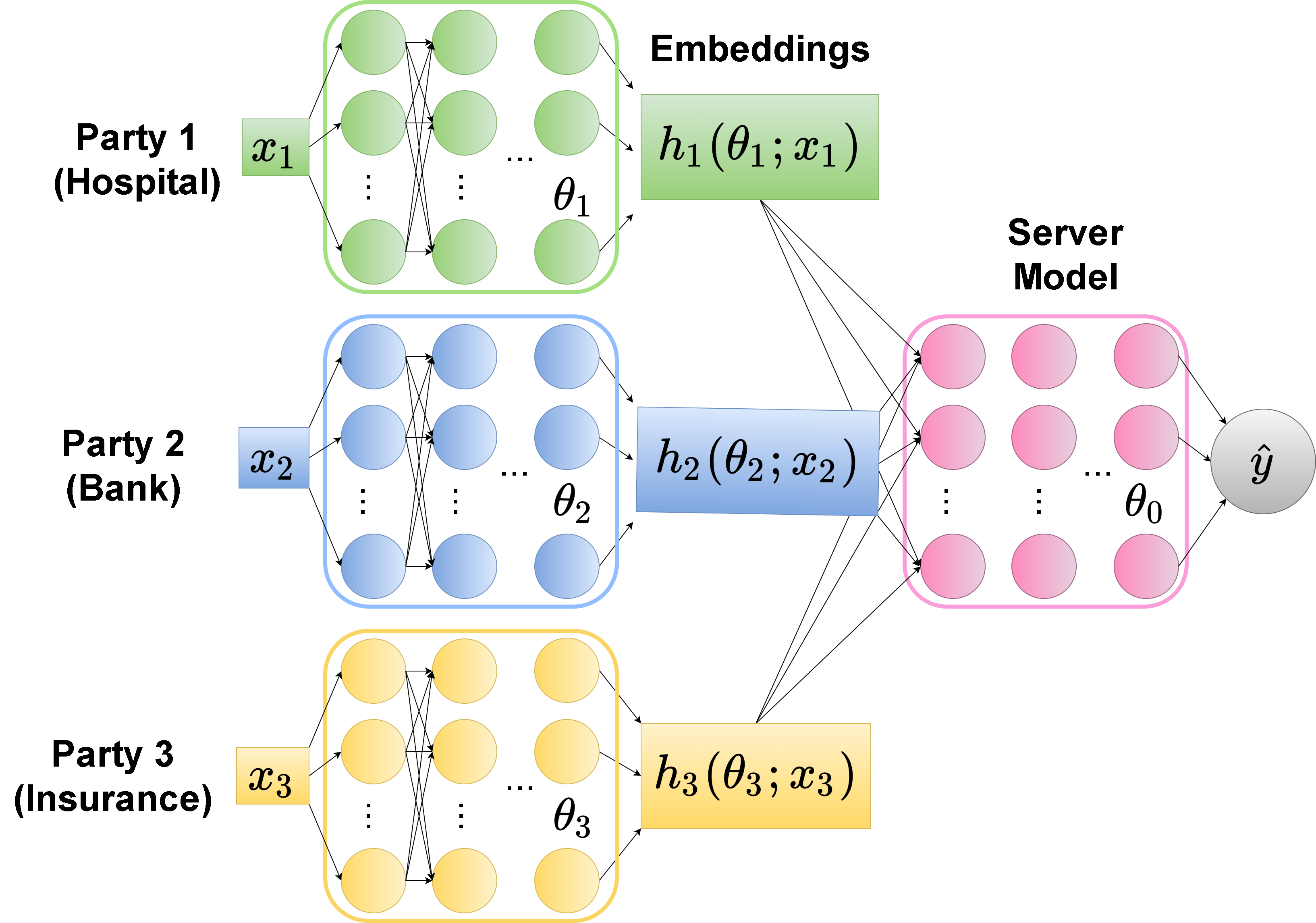
Typically in VFL, each party trains a local embedding function that maps raw data features to a meaningful vector representation, or embedding, for prediction tasks. For example, a neural network can be an embedding function for mapping the text of an online article to a vector space for classification (Koehrsen, 2018). Referring to Figure 1, suppose Party 111 is a hospital with medical data features x1subscript𝑥1x_{1}. The hospital computes its embedding h1(θ1;x1)subscript1subscript𝜃1subscript𝑥1h_{1}(\theta_{1};x_{1}) for the features by feeding x1subscript𝑥1x_{1} through a neural network. The other parties (the bank and insurance company), compute embeddings for their features, then all parties share the embeddings in a private manner (e.g., homomorphic encryption, secure multi-party computation, or secure aggregation). The embeddings are then combined in a server model θ0subscript𝜃0\theta_{0} to determine the final loss of the global model. A server model (or fusion network) captures the complicated interactions of embeddings and is often a complex, non-linear model (Gu et al., 2019; Nie et al., 2021; Han et al., 2021b). Embeddings can be very large, in practice, sometimes requiring terabytes of communication over the course of training.
Refer to caption
Figure 1: Example global model with neural networks. To obtain a y^^𝑦\hat{y} prediction for a data sample x𝑥x, each party m𝑚m feeds the local features of x𝑥x, xmsubscript𝑥𝑚x_{m}, into a neural network. The output of this neural network is the embedding hm(θm;xm)subscript𝑚subscript𝜃𝑚subscript𝑥𝑚h_{m}(\theta_{m};x_{m}). All embeddings are then fed into the server model neural network with parameters θ0subscript𝜃0\theta_{0}.

Motivated by this, we propose Compressed Vertical Federated Learning (C-VFL), a general framework for communication-efficient Federated Learning over vertically partitioned data. In our algorithm, parties communicate compressed embeddings periodically, and the parties and the server each run block-coordinate descent for multiple local iterations, in parallel, using stochastic gradients to update their local parameters.

C-VFL is the first theoretically verified VFL algorithm that applies embedding compression. Unlike in HFL algorithms, C-VFL compresses embeddings rather than gradients. Previous work has proven convergence for HFL algorithms with gradient compression (Stich et al., 2018; Wen et al., 2017; Karimireddy et al., 2019). However, no previous work analyzes the convergence requirements for VFL algorithms that use embedding compression. Embeddings are parameters in the partial derivatives calculated at each party. The effect of compression error on the resulting partial derivatives may be complex; therefore, the analysis in previous work on gradient compression in HFL does not apply to compression in VFL. In our work, we prove that, under a diminishing compression error, C-VFL converges at a rate of O(1T)𝑂1𝑇O(\frac{1}{\sqrt{T}}), which is comparable to previous VFL algorithms that do not employ compression. We also analyze common compressors, such as quantization and sparsification, in C-VFL and provide bounds on their compression parameters to ensure convergence.
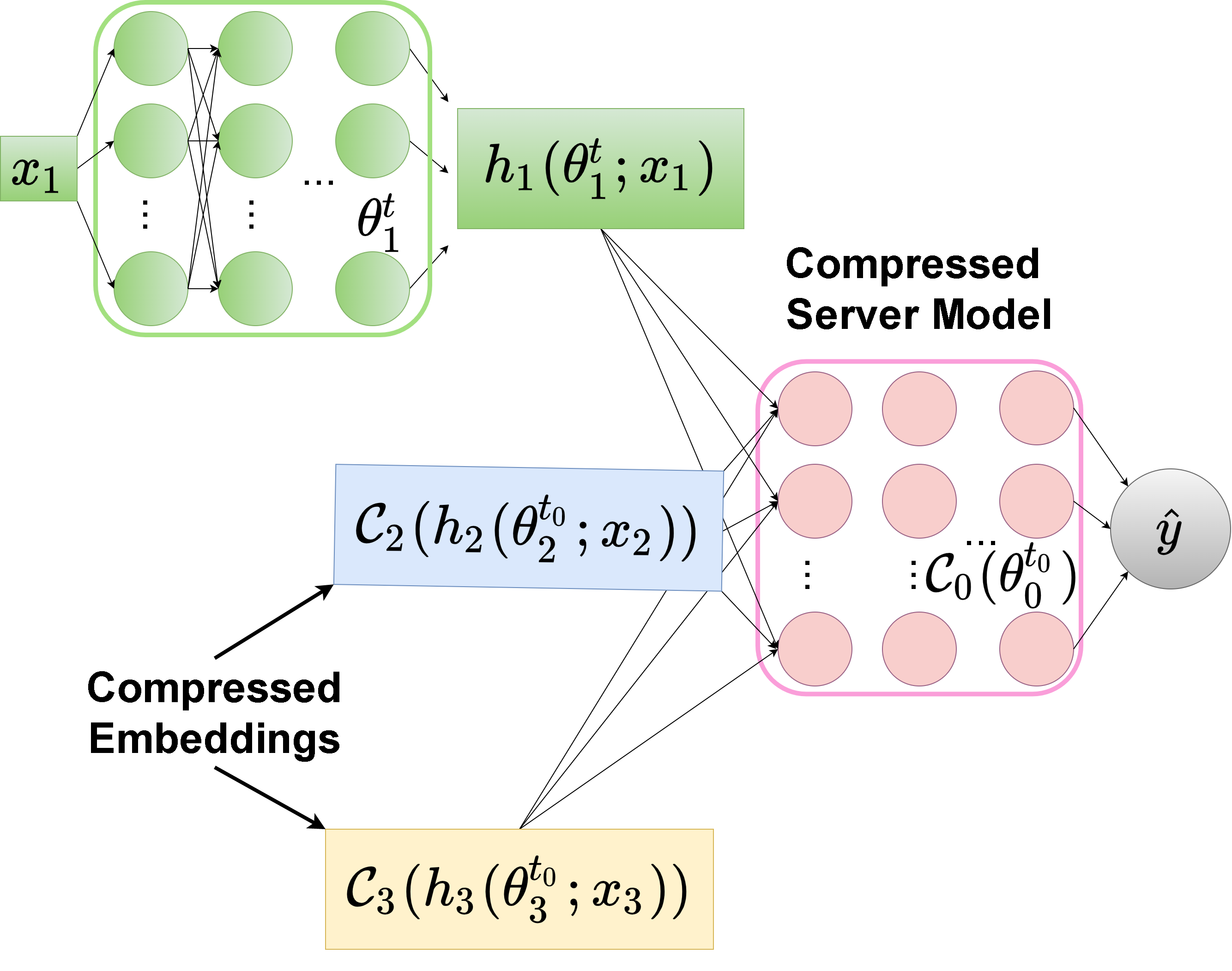
Refer to caption
Figure 2: Example local view of a global model with neural networks. When running C-VFL, Party 111 (in green) only has a compressed snapshot of the other parties embeddings and the server model. To calculate y^^𝑦\hat{y}, Party 111 uses its own embedding calculated at iteration t𝑡t, and the embeddings and server model calculated at time t0subscript𝑡0t_{0}, the latest communication iteration, and compressed with 𝒞msubscript𝒞𝑚\mathcal{C}_{m}.

C-VFL also generalizes previous work by supporting an arbitrary server model. Previous work in VFL has either only analyzed an arbitrary server model without local updates (Chen et al., 2020), or analyzed local updates with a linear server model (Liu et al., 2019; Zhang et al., 2020; Das & Patterson, 2021). C-VFL is designed with an arbitrary server model, allowing support for more complex prediction tasks than those supported by previous VFL algorithms.

We summarize our main contributions in this work.

  1. 1.

    We introduce C-VFL with an arbitrary compression scheme. Our algorithm generalizes previous work in VFL by including both an arbitrary server model and multiple local iterations.

  2. 2.

    We prove convergence of C-VFL to a neighborhood of a fixed point on non-convex objectives at a rate of O(1T)𝑂1𝑇O(\frac{1}{\sqrt{T}}) for a fixed step size when the compression error is bounded over the course of training. We also prove that the algorithm convergence error goes to zero for a diminishing step size if the compression error diminishes as well. Our work provides novel analysis for the effect of compressing embeddings on convergence in a VFL algorithm. Our analysis also applies to Split Learning when uploads to the server are compressed.

  3. 3.

    We provide convergence bounds on parameters in common compressors that can be used in C-VFL. In particular, we examine scalar quantization (Bennett, 1948), lattice vector quantization (Zamir & Feder, 1996), and top-k𝑘k sparsification (Lin et al., 2018).

  4. 4.

    We evaluate our algorithm by training on MIMIC-III, CIFAR-10, and ModelNet10 datasets. We empirically show how C-VFL can reduce the number of bits sent by over 90%percent9090\% compared to VFL with no compression without a significant loss in accuracy of the final model.

Related Work.

(Richtárik & Takác, 2016; Hardy et al., 2017) were the first works to propose Federated Learning algorithms for vertically partitioned data. (Chen et al., 2020; Romanini et al., 2021) propose the inclusion of an arbitrary server model in a VFL algorithm. However, these works do not consider multiple local iterations, and thus communicate at every iteration. (Liu et al., 2019), (Feng & Yu, 2020), and (Das & Patterson, 2021) all propose different VFL algorithms with local iterations for vertically partitioned data but do not consider an arbitrary server model. Split Learning is a related concept to VFL (Gupta & Raskar, 2018). Split Learning can be thought of a special case of VFL when there is only one party. Recent works (He et al., 2020; Han et al., 2021a) have extended Split Learning to a Federated Learning setting. However, these works focus on the HFL setting and do not apply message compression. In contrast to previous works, our work addresses a vertical scenario, an arbitrary server model, local iterations, and message compression.

Message compression is a common topic in HFL scenarios, where participants exchange gradients determined by their local datasets. Methods of gradient compression in HFL include scalar quantization (Bernstein et al., 2018), vector quantization (Shlezinger et al., 2021), and top-k𝑘k sparsification (Shi et al., 2019). In C-VFL, compressed embeddings are shared, rather than compressed gradients. Analysis in previous work on gradient compression in HFL does not apply to compression in VFL, as the effect of embedding compression error on each party’s partial derivatives may be complex. No prior work has analyzed the impact of compression on convergence in VFL.

Outline.

In Section 2, we provide the problem formulation and our assumptions. Section 3 presents the details of C-VFL. In Section 4, we present our main theoretical results. Our experimental results are given in Section 5. Finally, we conclude in Section 6.

2 Problem Formulation

We present our problem formulation and notation to be used in the rest of the paper. We let anorm𝑎\left\|a\right\| be the 2-norm of a vector a𝑎a, and let AsubscriptnormA\left\|\operatorname{\textbf{A}}\right\|_{\mathcal{F}} be the Frobenius norm of a matrix AA\operatorname{\textbf{A}}.

We consider a set of M𝑀M parties {1,,M}1𝑀\{1,\ldots,M\} and a server. The dataset XN×DXsuperscript𝑁𝐷\operatorname{\textbf{X}}\in\mathbb{R}^{N\times D} is vertically partitioned a priori across the M𝑀M parties, where N𝑁N is the number of data samples and D𝐷D is the number of features. The i𝑖i-th row of XX\operatorname{\textbf{X}} corresponds to a data sample xisuperscript𝑥𝑖x^{i}. For each sample xisuperscript𝑥𝑖x^{i}, a party m𝑚m holds a disjoint subset of the features, denoted xmisuperscriptsubscript𝑥𝑚𝑖x_{m}^{i}, so that xi=[x1i,,xMi]superscript𝑥𝑖superscriptsubscript𝑥1𝑖superscriptsubscript𝑥𝑀𝑖x^{i}=[x_{1}^{i},\ldots,x_{M}^{i}]. For each xisuperscript𝑥𝑖x^{i}, there is a corresponding label yisuperscript𝑦𝑖y^{i}. Let yN×1ysuperscript𝑁1\operatorname{\textbf{y}}\in\mathbb{R}^{N\times 1} be the vector of all sample labels. We let XmN×DmsubscriptX𝑚superscript𝑁subscript𝐷𝑚\operatorname{\textbf{X}}_{m}\in\mathbb{R}^{N\times D_{m}} be the local dataset of a party m𝑚m, where the i𝑖i-th row correspond to data features xmisuperscriptsubscript𝑥𝑚𝑖x_{m}^{i}. We assume that the server and all parties have a copy of the labels yy\operatorname{\textbf{y}}. For scenarios where the labels are private and only present at a single party, the label holder can provide enough information for the parties to compute gradients for some classes of model architectures (Liu et al., 2019).

Each party m𝑚m holds a set of model parameters θmsubscript𝜃𝑚\theta_{m} as well as a local embedding function hm()subscript𝑚h_{m}(\cdot). The server holds a set of parameters θ0subscript𝜃0\theta_{0} called the server model and a loss function l()𝑙l(\cdot) that combines the embeddings hm(θm;xmi)subscript𝑚subscript𝜃𝑚superscriptsubscript𝑥𝑚𝑖h_{m}(\theta_{m};x_{m}^{i}) from all parties. Our objective is to minimize the following:

F(Θ;X;y)𝐹ΘXy\displaystyle F(\Theta;\operatorname{\textbf{X}};\operatorname{\textbf{y}})
1Ni=1Nl(θ0,h1(θ1;x1i),,hM(θM;xMi);yi)absent1𝑁superscriptsubscript𝑖1𝑁𝑙subscript𝜃0subscript1subscript𝜃1subscriptsuperscript𝑥𝑖1subscript𝑀subscript𝜃𝑀subscriptsuperscript𝑥𝑖𝑀superscript𝑦𝑖\displaystyle~{}~{}~{}~{}~{}\coloneqq\frac{1}{N}\sum_{i=1}^{N}l(\theta_{0},h_{1}(\theta_{1};x^{i}_{1}),\ldots,h_{M}(\theta_{M};x^{i}_{M});y^{i}) (1)

where Θ=[θ0T,,θMT]TΘsuperscriptsuperscriptsubscript𝜃0𝑇superscriptsubscript𝜃𝑀𝑇𝑇\Theta=[\theta_{0}^{T},\ldots,\theta_{M}^{T}]^{T} is the global model. An example of a global model ΘΘ\Theta is in Figure 1.

For simplicity, we let m=0𝑚0m=0 refer to the server, and define h0(θ0;xi)θ0subscript0subscript𝜃0superscript𝑥𝑖subscript𝜃0h_{0}(\theta_{0};x^{i})\coloneqq\theta_{0} for all xisuperscript𝑥𝑖x^{i}, where h0()subscript0h_{0}(\cdot) is equivalent to the identity function. Let hm(θm;xmi)Pmsubscript𝑚subscript𝜃𝑚subscriptsuperscript𝑥𝑖𝑚superscriptsubscript𝑃𝑚h_{m}(\theta_{m};x^{i}_{m})\in\mathbb{R}^{P_{m}} for m=0,,M𝑚0𝑀m=0,\ldots,M, where Pmsubscript𝑃𝑚P_{m} is the size of the m𝑚m-th embedding. Let mF(Θ;X;y)1Ni=1Nθml(θ0,h1(θ1;x1i),,hM(θM;xMi);yi)subscript𝑚𝐹ΘXy1𝑁superscriptsubscript𝑖1𝑁subscriptsubscript𝜃𝑚𝑙subscript𝜃0subscript1subscript𝜃1subscriptsuperscript𝑥𝑖1subscript𝑀subscript𝜃𝑀subscriptsuperscript𝑥𝑖𝑀superscript𝑦𝑖\nabla_{m}F(\Theta;\operatorname{\textbf{X}};\operatorname{\textbf{y}})\coloneqq\frac{1}{N}\sum_{i=1}^{N}\nabla_{\theta_{m}}l(\theta_{0},h_{1}(\theta_{1};x^{i}_{1}),\ldots,h_{M}(\theta_{M};x^{i}_{M});y^{i}) be the partial derivatives for parameters θmsubscript𝜃𝑚\theta_{m}.

Let XBsuperscriptXB\operatorname{\textbf{X}}^{\operatorname{\textbf{B}}} and yBsuperscriptyB\operatorname{\textbf{y}}^{\operatorname{\textbf{B}}} be the set of samples and labels corresponding to a randomly sampled mini-batch BB\operatorname{\textbf{B}} of size B𝐵B. We let the stochastic partial derivatives for parameters θmsubscript𝜃𝑚\theta_{m} be mFB(Θ;X;y)1Bxi,yiXB,yBθml(θ0,h1(θ1;x1i),,hM(θM;xMi);y)subscript𝑚subscript𝐹BΘXy1𝐵subscriptformulae-sequencesuperscript𝑥𝑖superscript𝑦𝑖superscriptXBsuperscriptyBsubscriptsubscript𝜃𝑚𝑙subscript𝜃0subscript1subscript𝜃1subscriptsuperscript𝑥𝑖1subscript𝑀subscript𝜃𝑀subscriptsuperscript𝑥𝑖𝑀𝑦\nabla_{m}F_{\operatorname{\textbf{B}}}(\Theta;\operatorname{\textbf{X}};\operatorname{\textbf{y}})\coloneqq\frac{1}{B}\sum_{x^{i},y^{i}\in\operatorname{\textbf{X}}^{\operatorname{\textbf{B}}},\operatorname{\textbf{y}}^{\operatorname{\textbf{B}}}}\nabla_{\theta_{m}}l(\theta_{0},h_{1}(\theta_{1};x^{i}_{1}),\ldots,h_{M}(\theta_{M};x^{i}_{M});y). We may drop XX\operatorname{\textbf{X}} and yy\operatorname{\textbf{y}} from F()𝐹F(\cdot) and FB()subscript𝐹BF_{\operatorname{\textbf{B}}}(\cdot). With a minor abuse of notation, we let hm(θm;XmB){hm(θm;xmB1),,hm(θm;xmBB)}subscript𝑚subscript𝜃𝑚superscriptsubscriptX𝑚Bsubscript𝑚subscript𝜃𝑚subscriptsuperscript𝑥superscriptB1𝑚subscript𝑚subscript𝜃𝑚subscriptsuperscript𝑥superscriptB𝐵𝑚h_{m}(\theta_{m};\operatorname{\textbf{X}}_{m}^{\operatorname{\textbf{B}}})\coloneqq\{h_{m}(\theta_{m};x^{\operatorname{\textbf{B}}^{1}}_{m}),\ldots,h_{m}(\theta_{m};x^{\operatorname{\textbf{B}}^{B}}_{m})\} be the set of all party m𝑚m embeddings associated with mini-batch BB\operatorname{\textbf{B}}, where BisuperscriptB𝑖\operatorname{\textbf{B}}^{i} is the i𝑖i-th sample in the mini-batch BB\operatorname{\textbf{B}}. We let mFB(Θ)subscript𝑚subscript𝐹BΘ\nabla_{m}F_{\operatorname{\textbf{B}}}(\Theta) and mFB(θ0,h1(θ1;X1B),,hM(θM;XMB))subscript𝑚subscript𝐹Bsubscript𝜃0subscript1subscript𝜃1superscriptsubscriptX1Bsubscript𝑀subscript𝜃𝑀superscriptsubscriptX𝑀B\nabla_{m}F_{\operatorname{\textbf{B}}}(\theta_{0},h_{1}(\theta_{1};\operatorname{\textbf{X}}_{1}^{\operatorname{\textbf{B}}}),\ldots,h_{M}(\theta_{M};\operatorname{\textbf{X}}_{M}^{\operatorname{\textbf{B}}})) be equivalent, and use them interchangeably.

Assumption 1.

Smoothness: There exists positive constants L<𝐿{L<\infty} and Lm<subscript𝐿𝑚{L_{m}<\infty}, for m=0,,M𝑚0𝑀{m=0,\ldots,M}, such that for all Θ1subscriptΘ1\Theta_{1}, Θ2subscriptΘ2\Theta_{2}, the objective function satisfies:

F(Θ1)F(Θ2)norm𝐹subscriptΘ1𝐹subscriptΘ2\displaystyle\left\|\nabla F(\Theta_{1})-\nabla F(\Theta_{2})\right\| LΘ1Θ2absent𝐿normsubscriptΘ1subscriptΘ2\displaystyle\leq L\left\|\Theta_{1}-\Theta_{2}\right\|
mFB(Θ1)mFB(Θ2)normsubscript𝑚subscript𝐹BsubscriptΘ1subscript𝑚subscript𝐹BsubscriptΘ2\displaystyle\left\|\nabla_{m}F_{\operatorname{\textbf{B}}}(\Theta_{1})-\nabla_{m}F_{\operatorname{\textbf{B}}}(\Theta_{2})\right\| LmΘ1Θ2.absentsubscript𝐿𝑚normsubscriptΘ1subscriptΘ2\displaystyle\leq L_{m}\left\|\Theta_{1}-\Theta_{2}\right\|.
Assumption 2.

Unbiased gradients: For m=0,,M𝑚0𝑀m=0,\ldots,M, for every mini-batch BB\operatorname{\textbf{B}}, the stochastic partial derivatives are unbiased, i.e., 𝔼BmFB(Θ)=mF(Θ)subscript𝔼Bsubscript𝑚subscript𝐹BΘsubscript𝑚𝐹Θ\mathbb{E}_{\operatorname{\textbf{B}}}{\nabla_{m}F_{\operatorname{\textbf{B}}}(\Theta)}=\nabla_{m}F(\Theta).

Assumption 3.

Bounded variance: For m=0,,M𝑚0𝑀m=0,\ldots,M, there exists constants σm<subscript𝜎𝑚{\sigma_{m}<\infty} such that the variance of the stochastic partial derivatives are bounded as: 𝔼BmF(Θ)mFB(Θ)2σm2Bsubscript𝔼Bsuperscriptnormsubscript𝑚𝐹Θsubscript𝑚subscript𝐹BΘ2superscriptsubscript𝜎𝑚2𝐵\mathbb{E}_{\operatorname{\textbf{B}}}{\left\|\nabla_{m}F(\Theta)-\nabla_{m}F_{\operatorname{\textbf{B}}}(\Theta)\right\|^{2}}\leq\frac{\sigma_{m}^{2}}{B} for a mini-batch BB\operatorname{\textbf{B}} of size B𝐵B.

Assumption 1 bounds how fast the gradient and stochastic partial derivatives can change. Assumptions 2 and 3 require that the stochastic partial derivatives are unbiased estimators of the true partial derivatives with bounded variance. Assumptions 13 are common assumptions in convergence analysis of gradient-based algorithms (Tsitsiklis et al., 1986; Nguyen et al., 2018; Bottou et al., 2018). We note Assumptions 23 are similar to the IID assumptions in HFL convergence analysis. However, in VFL settings, all parties store identical sample IDs but different subsets of features. Hence, there is no equivalent notion of a non-IID distribution in VFL.

Assumption 4.

Bounded Hessian: There exists positive constants Hmsubscript𝐻𝑚H_{m} for m=0,,M𝑚0𝑀m=0,\ldots,M such that for all ΘΘ\Theta, the second partial derivatives of FBsubscript𝐹BF_{\operatorname{\textbf{B}}} with respect to hm(θm;XmB)subscript𝑚subscript𝜃𝑚superscriptsubscriptX𝑚Bh_{m}(\theta_{m};\operatorname{\textbf{X}}_{m}^{\operatorname{\textbf{B}}}) satisfy:

hm(θm;XmB)2FB(Θ)Hmsubscriptnormsubscriptsuperscript2subscript𝑚subscript𝜃𝑚superscriptsubscriptX𝑚Bsubscript𝐹BΘsubscript𝐻𝑚\displaystyle\|\nabla^{2}_{h_{m}(\theta_{m};\operatorname{\textbf{X}}_{m}^{\operatorname{\textbf{B}}})}F_{\operatorname{\textbf{B}}}(\Theta)\|_{\mathcal{F}}\leq H_{m} (2)

for any mini-batch BB\operatorname{\textbf{B}}.

Assumption 5.

Bounded Embedding Gradients: There exists positive constants Gmsubscript𝐺𝑚G_{m} for m=0,,M𝑚0𝑀m=0,\ldots,M such that for all θmsubscript𝜃𝑚\theta_{m}, the stochastic embedding gradients are bounded:

θmhm(θm;XmB)Gmsubscriptnormsubscriptsubscript𝜃𝑚subscript𝑚subscript𝜃𝑚superscriptsubscriptX𝑚Bsubscript𝐺𝑚\displaystyle\|\nabla_{\theta_{m}}h_{m}(\theta_{m};\operatorname{\textbf{X}}_{m}^{\operatorname{\textbf{B}}})\|_{\mathcal{F}}\leq G_{m} (3)

for any mini-batch BB\operatorname{\textbf{B}}.

Since we are assuming a Lipschitz-continuous loss function (Assumption 1), we know the Hessian of F𝐹F is bounded. Assumption 4 strengthens this assumption slightly to also bound the Hessian over any mini-batch. Assumption 5 bounds the magnitude of the partial derivatives with respect to embeddings. This embedding gradient bound is necessary to ensure convergence in the presence of embedding compression error (see Appendix A.2 for details).

3 Algorithm

We now present C-VFL, a communication-efficient method for training a global model with vertically partitioned data. In each global round, a mini-batch BB\operatorname{\textbf{B}} is chosen randomly from all samples and parties share necessary information for local training on this mini-batch. Each party m𝑚m, in parallel, runs block-coordinate stochastic gradient descent on its local model parameters θmsubscript𝜃𝑚\theta_{m} for Q𝑄Q local iterations. C-VFL runs for a total of R𝑅R global rounds, and thus runs for T=RQ𝑇𝑅𝑄T=RQ total local iterations.

For party m𝑚m to compute the stochastic gradient with respect to its features, it requires the embeddings computed by all other parties jm𝑗𝑚j\neq m. In C-VFL, these embeddings are shared with the server then distributed to the parties. We reduce communication cost by only sharing embeddings every global round. Further, each party compresses their embeddings before sharing. We define a set of general compressors for compressing party embeddings and the server model: 𝒞m():PmPm:subscript𝒞𝑚superscriptsubscript𝑃𝑚superscriptsubscript𝑃𝑚\mathcal{C}_{m}(\cdot):\mathbb{R}^{P_{m}}\rightarrow\mathbb{R}^{P_{m}} for m=0,,M𝑚0𝑀m=0,\ldots,M. To calculate the gradient for data sample xisuperscript𝑥𝑖x^{i}, party m𝑚m receives 𝒞j(hj(θj;xji))subscript𝒞𝑗subscript𝑗subscript𝜃𝑗superscriptsubscript𝑥𝑗𝑖\mathcal{C}_{j}(h_{j}(\theta_{j};x_{j}^{i})) from all parties jm𝑗𝑚j\neq m. With this information, a party m𝑚m can compute mFBsubscript𝑚subscript𝐹B\nabla_{m}F_{\operatorname{\textbf{B}}} and update its parameters θmsubscript𝜃𝑚\theta_{m} for multiple local iterations. Note that each party uses a stale view of the global model to compute its gradient during these local iterations, as it is reusing the embeddings it receives at the start of the round. In Section 4, we show that C-VFL converges even though parties use stale information. An example view a party has of the global model during training is in Figure 2. Here, t𝑡t is the current iteration and t0subscript𝑡0t_{0} is the start of the most recent global round, when embeddings were shared.

1:  Initialize: θm0superscriptsubscript𝜃𝑚0\theta_{m}^{0} for all parties m𝑚m and server model θ00superscriptsubscript𝜃00\theta_{0}^{0}
2:  for t0,,T1𝑡0𝑇1t\leftarrow 0,\ldots,T-1 do
3:     if t𝑡t mod Q=0𝑄0Q=0 then
4:        Randomly sample Bt{X,y}superscriptB𝑡Xy\operatorname{\textbf{B}}^{t}\in\{\operatorname{\textbf{X}},\operatorname{\textbf{y}}\}
5:        for m1,,M𝑚1𝑀m\leftarrow 1,\ldots,M in parallel do
6:           Send 𝒞m(hm(θmt;XmBt))subscript𝒞𝑚subscript𝑚superscriptsubscript𝜃𝑚𝑡subscriptsuperscriptXsuperscriptB𝑡𝑚\mathcal{C}_{m}(h_{m}(\theta_{m}^{t};\operatorname{\textbf{X}}^{\operatorname{\textbf{B}}^{t}}_{m})) to server
7:        end for
8:        Φ^t0{𝒞0(θ0t),𝒞1(h1(θ1t)),,𝒞M(hM(θMt))}superscript^Φsubscript𝑡0subscript𝒞0superscriptsubscript𝜃0𝑡subscript𝒞1subscript1superscriptsubscript𝜃1𝑡subscript𝒞𝑀subscript𝑀superscriptsubscript𝜃𝑀𝑡\hat{\Phi}^{t_{0}}\leftarrow\{\mathcal{C}_{0}(\theta_{0}^{t}),\mathcal{C}_{1}(h_{1}(\theta_{1}^{t})),\ldots,\mathcal{C}_{M}(h_{M}(\theta_{M}^{t}))\}
9:        Server sends Φ^t0superscript^Φsubscript𝑡0\hat{\Phi}^{t_{0}} to all parties
10:     end if
11:     for m0,,M𝑚0𝑀m\leftarrow 0,\ldots,M in parallel do
12:        Φ^mt{Φ^mt0;hm(θmt;XmBt0)}superscriptsubscript^Φ𝑚𝑡superscriptsubscript^Φ𝑚subscript𝑡0subscript𝑚superscriptsubscript𝜃𝑚𝑡superscriptsubscriptX𝑚superscriptBsubscript𝑡0\hat{\Phi}_{m}^{t}\leftarrow\{\hat{\Phi}_{-m}^{t_{0}};h_{m}(\theta_{m}^{t};\operatorname{\textbf{X}}_{m}^{\operatorname{\textbf{B}}^{t_{0}}})\}
13:        θmt+1θmtηt0mFB(Φ^mt;yBt0)superscriptsubscript𝜃𝑚𝑡1superscriptsubscript𝜃𝑚𝑡superscript𝜂subscript𝑡0subscript𝑚subscript𝐹Bsuperscriptsubscript^Φ𝑚𝑡superscriptysuperscriptBsubscript𝑡0\theta_{m}^{t+1}\leftarrow\theta_{m}^{t}-\eta^{t_{0}}\nabla_{m}F_{\operatorname{\textbf{B}}}(\hat{\Phi}_{m}^{t};\operatorname{\textbf{y}}^{\operatorname{\textbf{B}}^{t_{0}}})
14:     end for
15:  end for
Algorithm 1 Compressed Vertical Federated Learning

Algorithm 1 details the procedure of C-VFL. In each global round, when t𝑡t mod Q=0𝑄0Q=0, a mini-batch BB\operatorname{\textbf{B}} is randomly sampled from XX\operatorname{\textbf{X}} and the parties exchange the associated embeddings, compressed using 𝒞m()subscript𝒞𝑚\mathcal{C}_{m}(\cdot), via the server (lines 3-9). Each party m𝑚m completes Q𝑄Q local iterations, using the compressed embeddings it received in iteration t0subscript𝑡0t_{0} and its own m𝑚m-th uncompressed embeddings hm(θmt,XmBt0)subscript𝑚superscriptsubscript𝜃𝑚𝑡superscriptsubscriptX𝑚superscriptBsubscript𝑡0h_{m}(\theta_{m}^{t},\operatorname{\textbf{X}}_{m}^{\operatorname{\textbf{B}}^{t_{0}}}). We denote the set of embeddings that each party receives in iteration t0subscript𝑡0t_{0} as:

Φ^t0{𝒞0(θ0t0),𝒞1(h1(θ1t0)),,𝒞M(hM(θMt0))}.superscript^Φsubscript𝑡0subscript𝒞0superscriptsubscript𝜃0subscript𝑡0subscript𝒞1subscript1superscriptsubscript𝜃1subscript𝑡0subscript𝒞𝑀subscript𝑀superscriptsubscript𝜃𝑀subscript𝑡0\displaystyle\hat{\Phi}^{t_{0}}\coloneqq\{\mathcal{C}_{0}(\theta_{0}^{t_{0}}),\mathcal{C}_{1}(h_{1}(\theta_{1}^{t_{0}})),\ldots,\mathcal{C}_{M}(h_{M}(\theta_{M}^{t_{0}}))\}. (4)

We let Φ^mt0superscriptsubscript^Φ𝑚subscript𝑡0\hat{\Phi}_{-m}^{t_{0}} be the set of compressed embeddings from parties jm𝑗𝑚j\neq m, and let Φ^mt{Φ^mt0;hm(θmt;XmBt0)}superscriptsubscript^Φ𝑚𝑡superscriptsubscript^Φ𝑚subscript𝑡0subscript𝑚superscriptsubscript𝜃𝑚𝑡superscriptsubscriptX𝑚superscriptBsubscript𝑡0\hat{\Phi}_{m}^{t}\coloneqq\{\hat{\Phi}_{-m}^{t_{0}};h_{m}(\theta_{m}^{t};\operatorname{\textbf{X}}_{m}^{\operatorname{\textbf{B}}^{t_{0}}})\}. For each local iteration, each party m𝑚m updates θmsubscript𝜃𝑚\theta_{m} by computing the stochastic partial derivatives mFB(Φ^mt;yBt0)subscript𝑚subscript𝐹Bsuperscriptsubscript^Φ𝑚𝑡superscriptysuperscriptBsubscript𝑡0\nabla_{m}F_{\operatorname{\textbf{B}}}(\hat{\Phi}_{m}^{t};\operatorname{\textbf{y}}^{\operatorname{\textbf{B}}^{t_{0}}}) and applying a gradient step with step size ηt0superscript𝜂subscript𝑡0\eta^{t_{0}} (lines 11-14).

A key difference of C-VFL from previous VFL algorithms is the support of a server model with trainable parameters, allowing for arbitrary fusion networks. To support such a model with multiple local iterations, the server model parameters are shared with the parties. Also note that the same mini-batch is used for all Q𝑄Q local iterations, thus communication is only required every Q𝑄Q iterations. Therefore, without any compression, the total communication cost is O(RM(BmPm+|θ0|))𝑂𝑅𝑀𝐵subscript𝑚subscript𝑃𝑚subscript𝜃0O(R\cdot M\cdot(B\cdot\sum_{m}P_{m}+|\theta_{0}|)) for R𝑅R global rounds. Our compression technique replaces Pmsubscript𝑃𝑚P_{m} and |θ0|subscript𝜃0|\theta_{0}| with smaller values based on the compression factor. For cases where embeddings, the batch size, and the server model are large, this reduction can greatly decrease the communication cost.

Privacy.

We now discuss privacy-preserving mechanisms for C-VFL. In HFL settings, model update or gradient information is shared in messages. It has been shown that gradients can leak information about the raw data (Phong et al., 2018; Geiping et al., 2020). However in C-VFL, parties only share embeddings and can only calculate the partial derivatives associated with the server model and their local models. Commonly proposed HFL gradient attacks cannot be performed on C-VFL. Embeddings may be vulnerable to model inversion attacks (Mahendran & Vedaldi, 2015), which are methods by which an attacker can recover raw input to a model using the embedding output and black-box access to the model. One can protect against such an attack using homomorphic encryption (Cheng et al., 2021; Hardy et al., 2017) or secure multi-party computation (Gu et al., 2021). Alternatively, if the input to the server model is the sum of party embeddings, then secure aggregation methods (Bonawitz et al., 2016) can be applied. Several works have proposed privacy-perserving methods for VFL settings (Cheng et al., 2021; Çatak, 2015; Zheng et al., 2022) that are compatible with the C-VFL algorithm.

Note that C-VFL assumes all parties have access to the labels. For low-risk scenarios, such as predicting credit score, labels may not need to be private among the parties. In cases where labels are private, one can augment C-VFL to apply the method in (Liu et al., 2019) for gradient calculation without the need for sharing labels. Our analysis in Section 4 would still hold in this case, and the additional communication is reduced by the use of message compression.

4 Analysis

Table 1: Choice of common compressor parameters to achieve a convergence rate of O(1/T)𝑂1𝑇O(1/\sqrt{T}). Pmsubscript𝑃𝑚P_{m} is the size of the m𝑚m-th embedding. In scalar quantization, we let there be 2qsuperscript2𝑞2^{q} quantization levels, and let hmaxsubscripth_{\max} and hminsubscripth_{\min} be respectively the maximum and minimum components in hm(θmt;xmi)subscript𝑚superscriptsubscript𝜃𝑚𝑡superscriptsubscript𝑥𝑚𝑖h_{m}(\theta_{m}^{t};x_{m}^{i}) for all iterations t𝑡t, parties m𝑚m, and xmisuperscriptsubscript𝑥𝑚𝑖x_{m}^{i}. We let V𝑉V be the size of the lattice cell in vector quantization. We let k𝑘k be the number of parameters sent in an embedding after top-k𝑘k sparsification, and (h2)maxsubscriptsuperscriptnorm2(\|h\|^{2})_{\max} be the maximum value of hm(θmt;xmi)2superscriptnormsubscript𝑚superscriptsubscript𝜃𝑚𝑡superscriptsubscript𝑥𝑚𝑖2\|h_{m}(\theta_{m}^{t};x_{m}^{i})\|^{2} for all iterations t𝑡t, parties m𝑚m, and xmisuperscriptsubscript𝑥𝑚𝑖x_{m}^{i}.
Scalar Quantization Vector Quantization Top-k𝑘k Sparsification
Parameter Choice q=Ω(log2(BPm(hmaxhmin)2T))𝑞Ωsubscript2𝐵subscript𝑃𝑚superscriptsubscriptsubscript2𝑇q=\Omega\left(\log_{2}\left(BP_{m}(h_{\max}-h_{\min})^{2}\sqrt{T}\right)\right) V=O(1BPmT)𝑉𝑂1𝐵subscript𝑃𝑚𝑇V=O\left(\frac{1}{BP_{m}\sqrt{T}}\right) k=Ω(PmPmB(h2)maxT)𝑘Ωsubscript𝑃𝑚subscript𝑃𝑚𝐵subscriptsuperscriptnorm2𝑇k=\Omega\left(P_{m}-\frac{P_{m}}{B(\left\|h\right\|^{2})_{\max}\sqrt{T}}\right)
Compression Error mt0BPm(hmaxhmin)21222qsuperscriptsubscript𝑚subscript𝑡0𝐵subscript𝑃𝑚superscriptsubscriptsubscript212superscript22𝑞\mathcal{E}_{m}^{t_{0}}\leq BP_{m}\frac{(h_{\max}-h_{\min})^{2}}{12}2^{-2q} mt0VBPm24superscriptsubscript𝑚subscript𝑡0𝑉𝐵subscript𝑃𝑚24\mathcal{E}_{m}^{t_{0}}\leq\frac{VBP_{m}}{24} mt0B(1kPm)(h2)maxsuperscriptsubscript𝑚subscript𝑡0𝐵1𝑘subscript𝑃𝑚subscriptsuperscriptnorm2\mathcal{E}_{m}^{t_{0}}\leq B(1-\frac{k}{P_{m}})(\|h\|^{2})_{\max}

In this section, we discuss our analytical approach and present our theoretical results. We first define the compression error associated with 𝒞m()subscript𝒞𝑚\mathcal{C}_{m}(\cdot):

Definition 4.1.

Compression Error: Let vectors ϵmxisuperscriptsubscriptitalic-ϵ𝑚superscript𝑥𝑖\epsilon_{m}^{x^{i}} for m=0,,M𝑚0𝑀m=0,\ldots,M, be the compression errors of 𝒞m()subscript𝒞𝑚\mathcal{C}_{m}(\cdot) on a data sample xisuperscript𝑥𝑖x^{i}: ϵmxi𝒞m(hm(θm;xi))hm(θm;xi)superscriptsubscriptitalic-ϵ𝑚superscript𝑥𝑖subscript𝒞𝑚subscript𝑚subscript𝜃𝑚superscript𝑥𝑖subscript𝑚subscript𝜃𝑚superscript𝑥𝑖\epsilon_{m}^{x^{i}}\coloneqq\mathcal{C}_{m}(h_{m}(\theta_{m};x^{i}))-h_{m}(\theta_{m};x^{i}). Let ϵmt0superscriptsubscriptitalic-ϵ𝑚subscript𝑡0\epsilon_{m}^{t_{0}} be the Pm×Bsubscript𝑃𝑚𝐵P_{m}\times B matrix with ϵmxisuperscriptsubscriptitalic-ϵ𝑚superscript𝑥𝑖\epsilon_{m}^{x^{i}} for all data samples xisuperscript𝑥𝑖x^{i} in mini-batch Bt0superscriptBsubscript𝑡0\operatorname{\textbf{B}}^{t_{0}} as the columns. We denote the expected squared message compression error from party m𝑚m at round t0subscript𝑡0t_{0} as mt0𝔼ϵmt02superscriptsubscript𝑚subscript𝑡0𝔼superscriptsubscriptnormsuperscriptsubscriptitalic-ϵ𝑚subscript𝑡02\mathcal{E}_{m}^{t_{0}}\coloneqq\mathbb{E}\left\|\epsilon_{m}^{t_{0}}\right\|_{\mathcal{F}}^{2}.

Let G^tsuperscript^G𝑡\hat{\operatorname{\textbf{G}}}^{t} be the stacked partial derivatives at iteration t𝑡t:

G^t[(0FB(Φ^0t;yBt0))T,,(MFB(Φ^Mt;yBt0))T]T.superscript^G𝑡superscriptsuperscriptsubscript0subscript𝐹Bsuperscriptsubscript^Φ0𝑡superscriptysuperscriptBsubscript𝑡0𝑇superscriptsubscript𝑀subscript𝐹Bsuperscriptsubscript^Φ𝑀𝑡superscriptysuperscriptBsubscript𝑡0𝑇𝑇\hat{\operatorname{\textbf{G}}}^{t}\coloneqq[(\nabla_{0}F_{\operatorname{\textbf{B}}}(\hat{\Phi}_{0}^{t};\operatorname{\textbf{y}}^{\operatorname{\textbf{B}}^{t_{0}}}))^{T},\ldots,(\nabla_{M}F_{\operatorname{\textbf{B}}}(\hat{\Phi}_{M}^{t};\operatorname{\textbf{y}}^{\operatorname{\textbf{B}}^{t_{0}}}))^{T}]^{T}.

The model ΘΘ\Theta evolves as:

Θt+1=Θtηt0G^t.superscriptΘ𝑡1superscriptΘ𝑡superscript𝜂subscript𝑡0superscript^G𝑡\displaystyle\Theta^{t+1}=\Theta^{t}-\eta^{t_{0}}\hat{\operatorname{\textbf{G}}}^{t}. (5)

We note the reuse of the mini-batch of Bt0superscriptBsubscript𝑡0\operatorname{\textbf{B}}^{t_{0}} for Q𝑄Q iterations in this recursion. This indicates that the stochastic gradients are not unbiased during local iterations t0+1tt0+Q1subscript𝑡01𝑡subscript𝑡0𝑄1t_{0}+1\leq t\leq t_{0}+Q-1. Using conditional expectation, we can apply Assumption 2 to the gradient calculated at iteration t0subscript𝑡0t_{0} when there is no compression error. We define Φt0superscriptΦsubscript𝑡0\Phi^{t_{0}} to be the set of embeddings that would be received by each party at iteration t0subscript𝑡0t_{0} if no compression error were applied:

Φt0superscriptΦsubscript𝑡0\displaystyle\Phi^{t_{0}} {θ0t0,h1(θ1t0),,hM(θMt0)}.absentsuperscriptsubscript𝜃0subscript𝑡0subscript1superscriptsubscript𝜃1subscript𝑡0subscript𝑀superscriptsubscript𝜃𝑀subscript𝑡0\displaystyle\coloneqq\{\theta_{0}^{t_{0}},h_{1}(\theta_{1}^{t_{0}}),\ldots,h_{M}(\theta_{M}^{t_{0}})\}. (6)

We let Φmt0superscriptsubscriptΦ𝑚subscript𝑡0\Phi_{-m}^{t_{0}} be the set of embeddings from parties jm𝑗𝑚j\neq m, and let Φmt{Φmt0;hm(θmt;XmBt0)}superscriptsubscriptΦ𝑚𝑡superscriptsubscriptΦ𝑚subscript𝑡0subscript𝑚superscriptsubscript𝜃𝑚𝑡superscriptsubscriptX𝑚superscriptBsubscript𝑡0\Phi_{m}^{t}\coloneqq\{\Phi_{-m}^{t_{0}};h_{m}(\theta_{m}^{t};\operatorname{\textbf{X}}_{m}^{\operatorname{\textbf{B}}^{t_{0}}})\}. Then, if we take expectation over Bt0superscriptBsubscript𝑡0\operatorname{\textbf{B}}^{t_{0}} conditioned on previous global models ΘtsuperscriptΘ𝑡\Theta^{t} up to t0subscript𝑡0t_{0}:

𝔼Bt0[mFB(Φmt0)|{Θτ}τ=0t0]=mF(Φmt0).subscript𝔼superscriptBsubscript𝑡0delimited-[]conditionalsubscript𝑚subscript𝐹BsuperscriptsubscriptΦ𝑚subscript𝑡0superscriptsubscriptsuperscriptΘ𝜏𝜏0subscript𝑡0subscript𝑚𝐹superscriptsubscriptΦ𝑚subscript𝑡0\displaystyle\mathbb{E}_{\operatorname{\textbf{B}}^{t_{0}}}[\nabla_{m}F_{\operatorname{\textbf{B}}}(\Phi_{m}^{t_{0}})~{}|~{}\{\Theta^{\tau}\}_{\tau=0}^{t_{0}}]=\nabla_{m}F(\Phi_{m}^{t_{0}}). (7)

With the help of (7), we can prove convergence by bounding the difference between the gradient at the start of each global round and those calculated during local iterations (see the proof of Lemma 2 in Appendix A.2 for details).

To account for compression error, using the chain rule and Taylor series expansion, we obtain:

Lemma 1.

Under Assumptions 4-5, the norm of the difference between the objective function value with compressed and uncompressed embeddings is bounded as:

𝔼mFB(Φ^mt)mFB(Φmt)2𝔼superscriptnormsubscript𝑚subscript𝐹Bsuperscriptsubscript^Φ𝑚𝑡subscript𝑚subscript𝐹BsuperscriptsubscriptΦ𝑚𝑡2\displaystyle\mathbb{E}\|\nabla_{m}F_{\operatorname{\textbf{B}}}(\hat{\Phi}_{m}^{t})-\nabla_{m}F_{\operatorname{\textbf{B}}}(\Phi_{m}^{t})\|^{2} Hm2Gm2j=0,jmMjt0.absentsuperscriptsubscript𝐻𝑚2superscriptsubscript𝐺𝑚2superscriptsubscriptformulae-sequence𝑗0𝑗𝑚𝑀superscriptsubscript𝑗subscript𝑡0\displaystyle\leq H_{m}^{2}G_{m}^{2}\sum_{j=0,j\neq m}^{M}\mathcal{E}_{j}^{t_{0}}.

The proof of Lemma 1 is given in Appendix A.2. Using Lemma 1, we can bound the effect of compression error on convergence.

We present our main theoretical results. All proofs are provided in Appendix A.

Theorem 4.2.

Convergence with fixed step size: Under Assumptions 1-5, if ηt0=ηsuperscriptηsubscriptt0η\eta^{t_{0}}=\eta for all iterations and satisfies ηt0116Qmax{L,maxmLm}superscriptηsubscriptt0116QLsubscriptmsubscriptLm\eta^{t_{0}}\leq\frac{1}{16Q\max\{L,\max_{m}L_{m}\}}, then the average squared gradient over RRR global rounds of Algorithm 1 is bounded:

1Rt0=0R1𝔼[F(Θt0)2]1𝑅superscriptsubscriptsubscript𝑡00𝑅1𝔼delimited-[]superscriptnorm𝐹superscriptΘsubscript𝑡02\displaystyle\frac{1}{R}\sum_{t_{0}=0}^{R-1}\mathbb{E}\left[\left\|\nabla F(\Theta^{t_{0}})\right\|^{2}\right]
4[F(Θ0)𝔼[F(ΘT)]]ηT+6ηQLm=0Mσm2Babsent4delimited-[]𝐹superscriptΘ0𝔼delimited-[]𝐹superscriptΘ𝑇𝜂𝑇6𝜂𝑄𝐿superscriptsubscript𝑚0𝑀superscriptsubscript𝜎𝑚2𝐵\displaystyle~{}~{}~{}~{}~{}~{}~{}\leq\frac{4\left[F(\Theta^{0})-\mathbb{E}\left[F(\Theta^{T})\right]\right]}{\eta T}+6\eta QL\sum_{m=0}^{M}\frac{\sigma_{m}^{2}}{B}
+92Q2Rm=0MHm2Gm2t0=0R1j=0,jmMjt0.92superscript𝑄2𝑅superscriptsubscript𝑚0𝑀superscriptsubscript𝐻𝑚2superscriptsubscript𝐺𝑚2superscriptsubscriptsubscript𝑡00𝑅1superscriptsubscriptformulae-sequence𝑗0𝑗𝑚𝑀superscriptsubscript𝑗subscript𝑡0\displaystyle~{}~{}~{}~{}~{}~{}~{}~{}~{}~{}~{}~{}~{}~{}~{}~{}~{}~{}~{}+\frac{92Q^{2}}{R}\sum_{m=0}^{M}H_{m}^{2}G_{m}^{2}\sum_{t_{0}=0}^{R-1}\sum_{j=0,j\neq m}^{M}\mathcal{E}_{j}^{t_{0}}. (8)

The first term in (8) is based on the difference between the initial model and final model of the algorithm. The second term is the error associated with the variance of the stochastic gradients and the Lipschitz constants L𝐿L and Lmsubscript𝐿𝑚L_{m}’s. The third term relates to the average compression error over all iterations. The larger the error introduced by a compressor, the larger the convergence error is. We note that setting jt0=0superscriptsubscript𝑗subscript𝑡00\mathcal{E}_{j}^{t_{0}}=0 for all parties and iterations provides an error bound on VFL without compression and is an improvement over the bound in (Liu et al., 2019) in terms of Q𝑄Q, M𝑀M, and B𝐵B. The second and third terms include a coefficient relating to local iterations. As the number of local iterations Q𝑄Q increases, the convergence error increases. However, increasing Q𝑄Q also has the effect of reducing the number of global rounds. Thus, it may be beneficial to have Q>1𝑄1Q>1 in practice. We explore this more in experiments in Section 5. The second and third terms scale with M𝑀M, the number of parties. However, VFL scenarios typically have a small number of parties (Kairouz et al., 2021), and thus M𝑀M plays a small role in convergence error. We note that when M=1𝑀1M=1 and Q=1𝑄1Q=1, Theorem 4.2 applies to Split Learning (Gupta & Raskar, 2018) when only uploads to the server are compressed.

Remark 4.3.

Let =1Rt0=0R1m=0Mmt01𝑅superscriptsubscriptsubscript𝑡00𝑅1superscriptsubscript𝑚0𝑀superscriptsubscript𝑚subscript𝑡0\mathcal{E}=\frac{1}{R}\sum_{t_{0}=0}^{R-1}\sum_{m=0}^{M}\mathcal{E}_{m}^{t_{0}}. If ηt0=1Tsuperscript𝜂subscript𝑡01𝑇\eta^{t_{0}}=\frac{1}{\sqrt{T}} for all global rounds t0subscript𝑡0t_{0}, for Q𝑄Q and B𝐵B independent of T𝑇T, then

1Rt0=0R1𝔼[F(Θt0)2]=O(1T+).1𝑅superscriptsubscriptsubscript𝑡00𝑅1𝔼delimited-[]superscriptnorm𝐹superscriptΘsubscript𝑡02𝑂1𝑇\frac{1}{R}{\sum_{t_{0}=0}^{R-1}}\mathbb{E}\left[\|\nabla F(\Theta^{t_{0}})\|^{2}\right]=O\left(\frac{1}{\sqrt{T}}+\mathcal{E}\right).

This indicates that if =O(1T)𝑂1𝑇\mathcal{E}=O(\frac{1}{\sqrt{T}}) then we can achieve a convergence rate of O(1T)𝑂1𝑇O(\frac{1}{\sqrt{T}}). Informally, this means that C-VFL can afford compression error and not worsen asymptotic convergence when this condition is satisfied. We discuss how this affects commonly used compressors in practice later in the section.

We consider a diminishing step size in the following:

Theorem 4.4.

Convergence with diminishing step size: Under Assumptions 1-5, if 0<ηt0<10superscriptηsubscriptt010<\eta^{t_{0}}<1 satisfies ηt0116Qmax{L,maxmLm}superscriptηsubscriptt0116QLsubscriptmsubscriptLm\eta^{t_{0}}\leq\frac{1}{16Q\max\{L,\max_{m}L_{m}\}}, then the minimum squared gradient over RRR global rounds of Algorithm 1 is bounded:

mint0=0,,R1𝔼[F(Θt0)2]=subscriptsubscript𝑡00𝑅1𝔼delimited-[]superscriptnorm𝐹superscriptΘsubscript𝑡02absent\displaystyle\min_{t_{0}=0,\ldots,R-1}\mathbb{E}\left[\left\|\nabla F(\Theta^{t_{0}})\right\|^{2}\right]=
O(1t0=0R1ηt0+t0=0R1(ηt0)2t=0T1ηt0+t0=0R1m=0Mηt0mt0t0=0R1ηt0).𝑂1superscriptsubscriptsubscript𝑡00𝑅1superscript𝜂subscript𝑡0superscriptsubscriptsubscript𝑡00𝑅1superscriptsuperscript𝜂subscript𝑡02superscriptsubscript𝑡0𝑇1superscript𝜂subscript𝑡0superscriptsubscriptsubscript𝑡00𝑅1superscriptsubscript𝑚0𝑀superscript𝜂subscript𝑡0superscriptsubscript𝑚subscript𝑡0superscriptsubscriptsubscript𝑡00𝑅1superscript𝜂subscript𝑡0\displaystyle O\left(\frac{1}{\sum_{t_{0}=0}^{R-1}\eta^{t_{0}}}+\frac{\sum_{t_{0}=0}^{R-1}(\eta^{t_{0}})^{2}}{\sum_{t=0}^{T-1}\eta^{t_{0}}}+\frac{\sum_{t_{0}=0}^{R-1}\sum_{m=0}^{M}\eta^{t_{0}}\mathcal{E}_{m}^{t_{0}}}{\sum_{t_{0}=0}^{R-1}\eta^{t_{0}}}\right).

If ηt0superscript𝜂subscript𝑡0\eta^{t_{0}} and mt0superscriptsubscript𝑚subscript𝑡0\mathcal{E}_{m}^{t_{0}} satisfy t0=0ηt0=superscriptsubscriptsubscript𝑡00superscript𝜂subscript𝑡0\sum_{t_{0}=0}^{\infty}\eta^{t_{0}}=\infty, t0=0(ηt0)2<superscriptsubscriptsubscript𝑡00superscriptsuperscript𝜂subscript𝑡02\sum_{t_{0}=0}^{\infty}(\eta^{t_{0}})^{2}<\infty, and t0=0m=0Mηt0mt0<superscriptsubscriptsubscript𝑡00superscriptsubscript𝑚0𝑀superscript𝜂subscript𝑡0superscriptsubscript𝑚subscript𝑡0\sum_{t_{0}=0}^{\infty}\sum_{m=0}^{M}\eta^{t_{0}}\mathcal{E}_{m}^{t_{0}}<\infty, then mint0=0,,R1𝔼[F(Θt0)2]0subscriptsubscript𝑡00𝑅1𝔼delimited-[]superscriptnorm𝐹superscriptΘsubscript𝑡020\min_{t_{0}=0,\ldots,R-1}\mathbb{E}\left[\left\|\nabla F(\Theta^{t_{0}})\right\|^{2}\right]\rightarrow 0 as R𝑅R\rightarrow\infty.

According to Theorem 4.4, the product of the step size and the compression error must be summable over all iterations. In the next subsection, we discuss how to choose common compressor parameters to ensure this property is satisified. We also see in Section 5 that good results can be achieved empirically without diminishing the step size or compression error.

Common Compressors.

In this section, we show how to choose common compressor parameters to achieve a convergence rate of O(1T)𝑂1𝑇O(\frac{1}{\sqrt{T}}) in the context of Theorem 4.2, and guarantee convergence in the context of Theorem 4.4. We analyze three common compressors: a uniform scalar quantizer (Bennett, 1948), a 222-dimensional hexagonal lattice quantizer (Zamir & Feder, 1996), and top-k𝑘k sparsification (Lin et al., 2018). For uniform scalar quantizer, we let there be 2qsuperscript2𝑞2^{q} quantization levels. For the lattice vector quantizer, we let V𝑉V be the volume of each lattice cell. For top-k𝑘k sparsification, we let k𝑘k be the number of embedding components sent in a message. In Table 1, we present the choice of compressor parameters in order to achieve a convergence rate of O(1T)𝑂1𝑇O(\frac{1}{\sqrt{T}}) in the context of Theorem 4.2. We show how we calculate these bounds in Appendix B and provide some implementation details for their use. We can also use Table 1 to choose compressor parameters to ensure convergence in the context of Theorem 4.4. Let ηt0=O(1t0)superscript𝜂subscript𝑡0𝑂1subscript𝑡0\eta^{t_{0}}=O(\frac{1}{t_{0}}), where t0subscript𝑡0t_{0} is the current round. Then setting T=t0𝑇subscript𝑡0T=t_{0} in Table 1 provides a choice of compression parameters at each iteration to ensure the compression error diminishes at a rate of O(1t0)𝑂1subscript𝑡0O(\frac{1}{\sqrt{t_{0}}}), guaranteeing convergence. Diminishing compression error can be achieved by increasing the number of quantization levels, decreasing the volume of lattice cells, or increasing the number of components sent in a message.

5 Experiments

We present experiments to examine the performance of C-VFL in practice. The goal of our experiments is to examine the effects that different compression techniques have on training, and investigate the accuracy/communication trade-off empirically. We run experiments on three datasets: the MIMIC-III dataset (Johnson et al., 2016), the ModelNet10 dataset (Wu et al., 2015), and the CIFAR-10 dataset (Krizhevsky et al., 2009). We provide more details on the datasets and training procedure in Appendix C, as well as additional plots and experiments in Appendix D.

MIMIC-III: MIMIC-III is an anonymized hospital patient time series dataset. In MIMIC-III, the task is binary classification to predict in-hospital mortality. We train with a set of 444 parties, each storing 191919 of the 767676 features. Each party trains an LSTM and the server trains two fully-connected layers. We use a fixed step size of 0.010.010.01, a batch size of 100010001000, and train for 100010001000 epochs.

CIFAR-10: CIFAR-10 is an image dataset for object classification. We train with a set of 444 parties, each storing a different quadrant of every image. Each party trains ResNet18, and the server trains a fully-connected layer. We use a fixed step size of 0.00010.00010.0001 and a batch size of 100100100, and train for 200200200 epochs.

ModelNet10: ModelNet10 is a set of CAD models, each with images of 121212 different camera views. The task of ModelNet10 is classification of images into 101010 object classes. We run experiments with both a set of 444 and 121212 parties, where parties receive 333 or 111 view(s) of each CAD model, respectively. Each party’s network consists of two convolutional layers and a fully-connected layer, and the server model consists of a fully-connected layer. We use a fixed step size of 0.0010.0010.001 and a batch size of 646464, and train for 100100100 epochs.

We consider the three compressors discussed in Section 4: a uniform scalar quantizer, a 222-dimensional hexagonal lattice (vector) quantizer, and top-k𝑘k sparsification. For both quantizers, the embedding values need to be bounded. In the case of the models used for MIMIC-III and CIFAR-10, the embedding values are already bounded, but the CNN used for ModelNet10 may have unbounded embedding values. We scale embedding values for ModelNet10 to the range [0,1]01[0,1]. We apply subtractive dithering to both the scalar quantizer (Wannamaker, 1997) and vector quantizer (Shlezinger et al., 2021).

In our experiments, each embedding component is a 323232-bit float. Let b𝑏b be the bits per component we compress to. For the scalar quantizer, this means there are 2bsuperscript2𝑏2^{b} quantization levels. For the 222-D vector quantizer, this means there are 22bsuperscript22𝑏2^{2b} vectors in the codebook. The volume V𝑉V of the vector quantizer is a function of the number of codebook vectors. For top-k𝑘k sparsification, k=Pmb32𝑘subscript𝑃𝑚𝑏32k=P_{m}\cdot\frac{b}{32} as we use 323232-bit components. We train using C-VFL and consider cases where b=2𝑏2b=2, 333, and 444. We compare with a case where b=32𝑏32b=32. This corresponds to a standard VFL algorithm without embedding compression (Liu et al., 2019), acting as a baseline for accuracy.
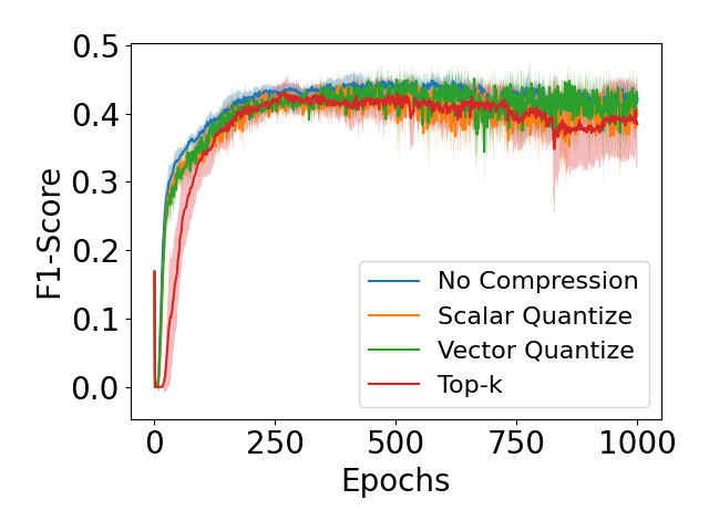
Refer to caption
(a) MIMIC-III by epochs
Refer to caption
(b) MIMIC-III by cost
Refer to caption
(c) CIFAR-10 by epochs
Refer to caption
(d) CIFAR-10 by cost
Refer to caption
(e) ModelNet10 by epochs
Refer to caption
(f) ModelNet10 by cost
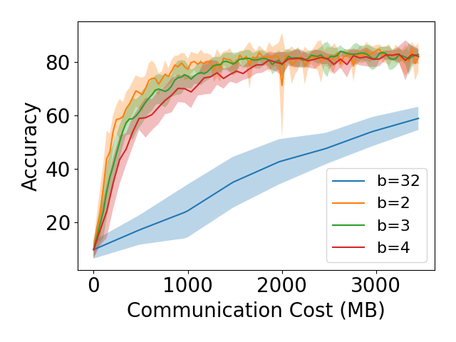
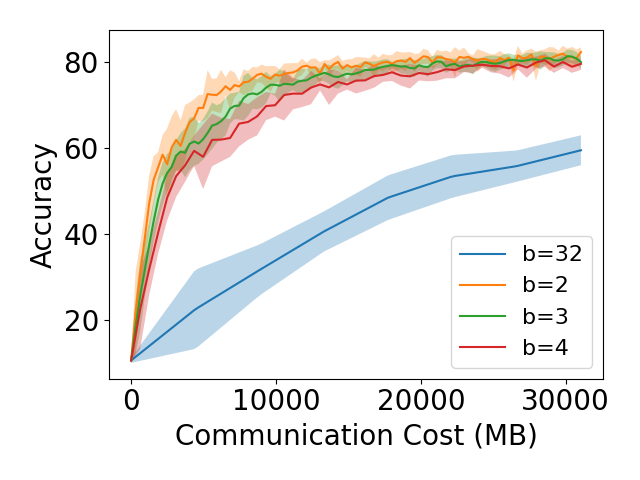
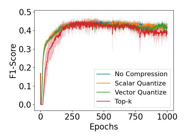
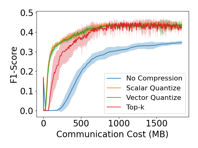
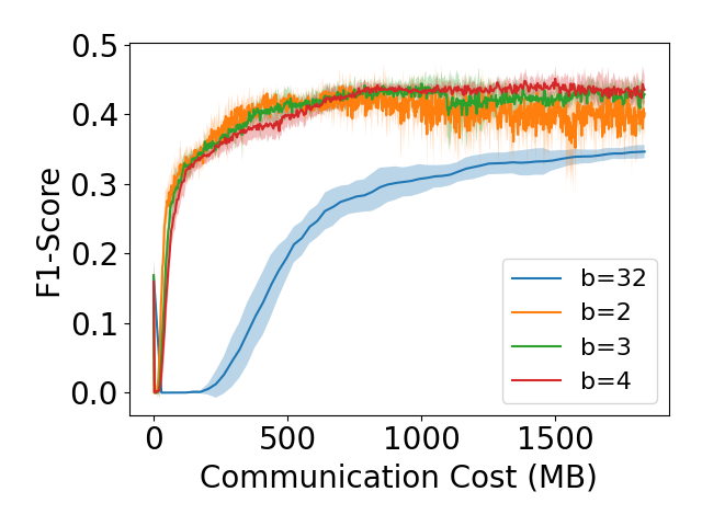
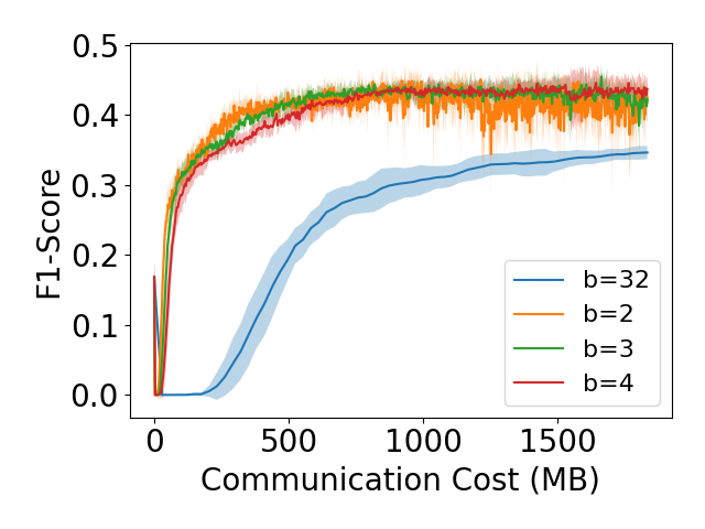
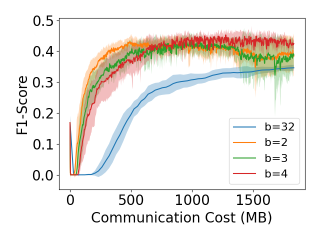
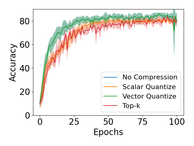
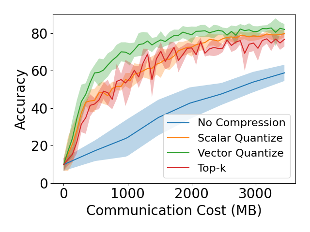
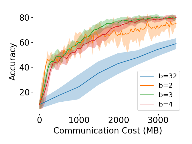
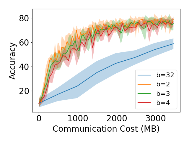
Figure 3: C-VFL when compressing to 222 bits per component. The solid lines are the mean of 555 runs, while the shaded region represents the standard deviation. We show test F1subscript𝐹1F_{1}-Score on MIMIC-III dataset and test accuracy on CIFAR-10 and ModelNet10 dataset, plotted by epochs and communication cost.

In Figure 3, we plot the test F1subscript𝐹1F_{1}-Score and test accuracy for MIMIC-III, CIFAR-10, and ModelNet10 when training with b=2𝑏2b=2. We use F1subscript𝐹1F_{1}-Score for MIMIC-III as the in-hospital mortality prediction task has high class imbalance; most people in the dataset did not die in the hospital. For these experiments, we let M=4𝑀4M=4 for ModelNet10. The solid line in each plot represents the average accuracy over five runs, while the shaded regions represent one standard deviation. In Figures 3(a), 3(c), and 3(e), we plot by the number of training epochs. We can see in all cases, although convergence can be a bit slower, training with compressed embeddings still reaches similar accuracy to no compression. In Figures 3(b), 3(d), and 3(f), we plot by the communication cost in bytes. The cost of communication includes both the upload of (compressed) embeddings to the server and download of embeddings and server model to all parties. We can see that by compressing embeddings, we can reach higher accuracy with significantly less communication cost. In all datasets, the compressors reach similar accuracy to each other, though top-k𝑘k sparsification performs slightly worse than the others on MIMIC-III, while vector quantization performs the best in both on CIFAR-10 and ModelNet10.

Table 2: MIMIC-III maximum F1subscript𝐹1F_{1}-Score reached during training, and communication cost to reach a target test F1subscript𝐹1F_{1}-Score of 0.40.40.4. Value shown is the mean of 555 runs, ±plus-or-minus\pm the standard deviation. In these experiments, Q=10𝑄10Q=10 and M=4𝑀4M=4.
Compressor Max F1subscript𝐹1F_{1}-Score Cost (MB)
Reached Target =0.4absent0.4=0.4
None b=32𝑏32b=32 0.448 ±plus-or-minus\pm 0.010 3830.0 ±plus-or-minus\pm 558.2
Scalar b=2𝑏2b=2 0.441 ±plus-or-minus\pm 0.018 233.1 ±plus-or-minus\pm 28.7
Vector b=2𝑏2b=2 0.451 ±plus-or-minus\pm 0.021 236.1 ±plus-or-minus\pm 17.9
Top-k𝑘k b=2𝑏2b=2 0.431 ±plus-or-minus\pm 0.016 309.8 ±plus-or-minus\pm 93.6
Scalar b=3𝑏3b=3 0.446 ±plus-or-minus\pm 0.011 343.1 ±plus-or-minus\pm 18.8
Vector b=3𝑏3b=3 0.455 ±plus-or-minus\pm 0.020 330.5 ±plus-or-minus\pm 10.6
Top-k𝑘k b=3𝑏3b=3 0.435 ±plus-or-minus\pm 0.030 470.7 ±plus-or-minus\pm 116.8
Scalar b=4𝑏4b=4 0.451 ±plus-or-minus\pm 0.020 456.0 ±plus-or-minus\pm 87.8
Vector b=4𝑏4b=4 0.446 ±plus-or-minus\pm 0.017 446.5 ±plus-or-minus\pm 21.3
Top-k𝑘k b=4𝑏4b=4 0.453 ±plus-or-minus\pm 0.014 519.1 ±plus-or-minus\pm 150.4
Table 3: CIFAR-10 maximum test accuracy reached during training, and communication cost to reach a target accuracy of 70%percent7070\%. Value shown is the mean of 555 runs, ±plus-or-minus\pm the standard deviation. A “–” indicates that the target was not reached during training. We let Q=10𝑄10Q=10 and M=4𝑀4M=4.
Compressor Max Accuracy Cost (GB)
Reached Target =70%absentpercent70=70\%
None b=32𝑏32b=32 73.18% ±plus-or-minus\pm 0.44% 7.69 ±plus-or-minus\pm 0.35
Scalar b=2𝑏2b=2 65.16% ±plus-or-minus\pm 1.85%
Vector b=2𝑏2b=2 71.43% ±plus-or-minus\pm 0.47% 0.68 ±plus-or-minus\pm 0.06
Top-k𝑘k b=2𝑏2b=2 66.02% ±plus-or-minus\pm 2.24%
Scalar b=3𝑏3b=3 71.49% ±plus-or-minus\pm 1.05% 1.22 ±plus-or-minus\pm 0.17
Vector b=3𝑏3b=3 72.50% ±plus-or-minus\pm 0.40% 0.81 ±plus-or-minus\pm 0.05
Top-k𝑘k b=3𝑏3b=3 71.56% ±plus-or-minus\pm 0.81% 1.24 ±plus-or-minus\pm 0.22
Scalar b=4𝑏4b=4 71.80% ±plus-or-minus\pm 1.18% 1.72 ±plus-or-minus\pm 0.26
Vector b=4𝑏4b=4 73.17% ±plus-or-minus\pm 0.39% 0.98 ±plus-or-minus\pm 0.08
Top-k𝑘k b=4𝑏4b=4 72.03% ±plus-or-minus\pm 1.77% 1.43 ±plus-or-minus\pm 0.26
Table 4: ModelNet10 maximum test accuracy reached during training, and communication cost to reach a target accuracy of 75%percent7575\%. Value shown is the mean of 555 runs, ±plus-or-minus\pm the standard deviation. We let Q=10𝑄10Q=10 and M=4𝑀4M=4.
Compressor Max Accuracy Cost (MB)
Reached Target =75%absentpercent75=75\%
None b=32𝑏32b=32 85.68% ±plus-or-minus\pm 1.57% 9604.80 ±plus-or-minus\pm 2933.40
Scalar b=2𝑏2b=2 76.94% ±plus-or-minus\pm 5.87% 1932.00 ±plus-or-minus\pm 674.30
Vector b=2𝑏2b=2 84.80% ±plus-or-minus\pm 2.58% 593.40 ±plus-or-minus\pm 170.98
Top-k𝑘k b=2𝑏2b=2 79.91% ±plus-or-minus\pm 2.86% 1317.90 ±plus-or-minus\pm 222.95
Scalar b=3𝑏3b=3 81.32% ±plus-or-minus\pm 1.61% 1738.80 ±plus-or-minus\pm 254.79
Vector b=3𝑏3b=3 85.66% ±plus-or-minus\pm 1.36% 900.45 ±plus-or-minus\pm 275.01
Top-k𝑘k b=3𝑏3b=3 81.63% ±plus-or-minus\pm 1.24% 1593.90 ±plus-or-minus\pm 225.34
Scalar b=4𝑏4b=4 81.19% ±plus-or-minus\pm 1.88% 2194.20 ±plus-or-minus\pm 266.88
Vector b=4𝑏4b=4 85.77% ±plus-or-minus\pm 1.69% 1200.60 ±plus-or-minus\pm 366.68
Top-k𝑘k b=4𝑏4b=4 83.50% ±plus-or-minus\pm 1.21% 1821.60 ±plus-or-minus\pm 241.40
Table 5: MIMIC-III time in seconds to reach a target F1subscript𝐹1F_{1}-Score for different local iterations Q𝑄Q and communication latency tcsubscript𝑡𝑐t_{c} with vector quantization and b=3𝑏3b=3. Value shown is the mean of 555 runs, ±plus-or-minus\pm one standard deviation.
tcsubscript𝑡𝑐t_{c} Time to Reach Target F1subscript𝐹1F_{1}-Score 0.450.450.45
Q=1𝑄1Q=1 Q=10𝑄10Q=10 Q=25𝑄25Q=25
111 694.53 ±plus-or-minus\pm 150.75 470.86 ±plus-or-minus\pm 235.35 445.21 ±plus-or-minus\pm 51.44
101010 1262.78 ±plus-or-minus\pm 274.10 512.82 ±plus-or-minus\pm 256.32 461.17 ±plus-or-minus\pm 53.29
505050 3788.32 ±plus-or-minus\pm 822.30 699.30 ±plus-or-minus\pm 349.53 532.12 ±plus-or-minus\pm 61.49
200200200 13259.14 ±plus-or-minus\pm 2878.04 1398.60 ±plus-or-minus\pm 699.05 798.19 ±plus-or-minus\pm 92.23

In Tables 2, 3 and 4, we show the maximum test accuracy reached during training and the communication cost to reach a target accuracy for MIMIC-III, CIFAR-10, and ModelNet10. We show results for all three compressors with b=2𝑏2b=2, 333, and 444 bits per component, as well as the baseline of b=32𝑏32b=32. For the MIMIC-III dataset, we show the maximum test F1subscript𝐹1F_{1}-Score reached and the total communication cost of reaching an F1subscript𝐹1F_{1}-Score of 0.40.40.4. The maximum F1subscript𝐹1F_{1}-Score for each case is within a standard deviation of each other. However, the cost to reach target score is much smaller as the value of b𝑏b decreases for all compressors. We can see that when b=2𝑏2b=2, we can achieve over 90%percent9090\% communication cost reduction over no compression to reach a target F1subscript𝐹1F_{1}-Score.

For the CIFAR-10 and ModelNet10 datasets, Tables 3 and 4 show the maximum test accuracy reached and the total communication cost of reaching a target accuracy. We can see that, for both datasets, vector quantization tends to outperform both scalar quantization and top-k𝑘k quantization. Vector quantization benefits from considering components jointly, and thus can have better reconstruction quality than scalar quantization and top-k𝑘k sparsification (Woods, 2006).

Refer to caption
(a) Parties M=4𝑀4M=4
Refer to caption
(b) Parties M=12𝑀12M=12
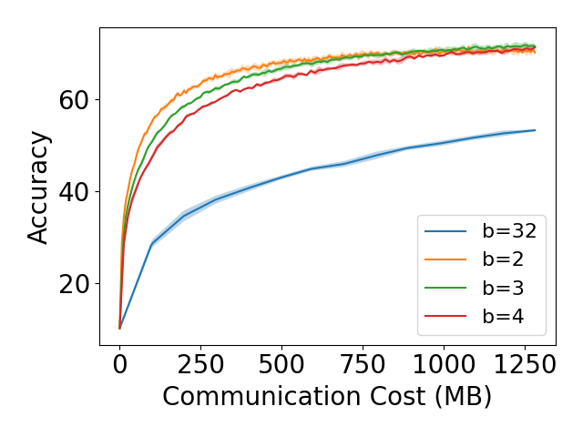
Figure 4: Communication cost of training on ModelNet10 with vector quantization. The solid lines are the mean of 555 runs, and the shaded region represents one standard deviation.

In Table 5, we consider the communication/computation tradeoff of local iterations. We show how the number of local iterations affects the time to reach a target F1subscript𝐹1F_{1}-Score in the MIMIC-III dataset. We train C-VFL with vector quantization b=3𝑏3b=3 and set the local iterations Q𝑄Q to 111, 101010, and 252525. Note that the Q=1𝑄1Q=1 case corresponds to adding embedding compression to previously proposed VFL algorithms that do not have multiple local iterations (Hu et al., 2019; Romanini et al., 2021). We simulate a scenario where computation time for training a mini-batch of data at each party takes 101010 ms, and communication of embeddings takes a total of 111, 101010, 505050, and 200200200 ms roundtrip. These different communication latencies correspond to the distance between the parties and the server: within the same cluster, on the same local network, within the same region, and across the globe. According to Theorem 4.2, increasing the number of local iterations Q𝑄Q increases convergence error. However, the target test accuracy is reached within less time when Q𝑄Q increases. The improvement over Q=1𝑄1Q=1 local iterations increases as the communication latency increases. In systems where communication latency is high, it may be beneficial to increase the number of local iterations. The choice of Q𝑄Q will depend on the accuracy requirements of the given prediction task and the time constraints on the prediction problem.

Finally, in Figure 4, we plot the test accuracy of ModelNet10 against the communication cost when using vector quantization with b=2𝑏2b=2, 333, 444, and 323232. We include plots for 444 and 121212 parties. We note that changing the number of parties changes the global model structure ΘΘ\Theta as well. We can see in both cases that smaller values of b𝑏b reach higher test accuracies at lower communication cost. The total communication cost is larger with 121212 parties, but the impact of increasing compression is similar for both M=4𝑀4M=4 and M=12𝑀12M=12.

6 Conclusion

We proposed C-VFL, a distributed communication-efficient algorithm for training a model over vertically partitioned data. We proved convergence of the algorithm at a rate of O(1T)𝑂1𝑇O(\frac{1}{\sqrt{T}}), and we showed experimentally that communication cost could be reduced by over 90%percent9090\% without a significant decrease in accuracy. For future work, we seek to relax our bounded gradient assumption and explore the effect of adaptive compressors.

Acknowledgements

This work was supported by the Rensselaer-IBM AI Research Collaboration (http://airc.rpi.edu), part of the IBM AI Horizons Network (http://ibm.biz/AIHorizons), and the National Science Foundation under grant CNS-1553340.

References

  • Bennett (1948) Bennett, W. R. Spectra of quantized signals. Bell Syst. Tech. J., 27(3):446–472, 1948.
  • Bernstein et al. (2018) Bernstein, J., Wang, Y., Azizzadenesheli, K., and Anandkumar, A. SIGNSGD: compressed optimisation for non-convex problems. Proc. Int. Conf. on Machine Learn., 2018.
  • Bonawitz et al. (2016) Bonawitz, K. A., Ivanov, V., Kreuter, B., Marcedone, A., McMahan, H. B., Patel, S., Ramage, D., Segal, A., and Seth, K. Practical secure aggregation for federated learning on user-held data. arXiv:1611.04482, 2016.
  • Bonawitz et al. (2019) Bonawitz, K. A., Eichner, H., Grieskamp, W., Huba, D., Ingerman, A., Ivanov, V., Kiddon, C., Konečný, J., Mazzocchi, S., McMahan, B., Overveldt, T. V., Petrou, D., Ramage, D., and Roselander, J. Towards federated learning at scale: System design. Proc. of Machine Learn. Sys., 2019.
  • Bottou et al. (2018) Bottou, L., Curtis, F. E., and Nocedal, J. Optimization methods for large-scale machine learning. SIAM Review, 60(2):223–311, 2018.
  • Çatak (2015) Çatak, F. Ö. Secure multi-party computation based privacy preserving extreme learning machine algorithm over vertically distributed data. Proc. Adv. Neural Inf. Process. Syst., 9490:337–345, 2015.
  • Ceballos et al. (2020) Ceballos, I., Sharma, V., Mugica, E., Singh, A., Roman, A., Vepakomma, P., and Raskar, R. Splitnn-driven vertical partitioning. arXiv:2008.04137, 2020.
  • Cha et al. (2021) Cha, D., Sung, M., and Park, Y.-R. Implementing vertical federated learning using autoencoders: Practical application, generalizability, and utility study. JMIR Medical Informatics, 9(6):e26598, 2021.
  • Chen et al. (2020) Chen, T., Jin, X., Sun, Y., and Yin, W. VAFL: a method of vertical asynchronous federated learning. arXiv:2007.06081, 2020.
  • Cheng et al. (2021) Cheng, K., Fan, T., Jin, Y., Liu, Y., Chen, T., Papadopoulos, D., and Yang, Q. Secureboost: A lossless federated learning framework. IEEE Intell. Syst., 36(6):87–98, 2021.
  • Das & Patterson (2021) Das, A. and Patterson, S. Multi-tier federated learning for vertically partitioned data. Proc. IEEE Int. Conf. on Acoust., Speech, and Signal Process., pp.  3100–3104, 2021.
  • Deng et al. (2009) Deng, J., Dong, W., Socher, R., Li, L.-J., Li, K., and Fei-Fei, L. Imagenet: A large-scale hierarchical image database. In Proc. IEEE Conf. Comput. Vis. Pattern Recognit., 2009.
  • Feng & Yu (2020) Feng, S. and Yu, H. Multi-participant multi-class vertical federated learning. arXiv:2001.11154, 2020.
  • Geiping et al. (2020) Geiping, J., Bauermeister, H., Dröge, H., and Moeller, M. Inverting gradients - how easy is it to break privacy in federated learning? Adv. Neural Inf. Process. Syst., 2020.
  • Gu et al. (2021) Gu, B., Xu, A., Huo, Z., Deng, C., and Huang, H. Privacy-preserving asynchronous vertical federated learning algorithms for multiparty collaborative learning. IEEE Trans. on Neural Netw. Learn. Syst., pp.  1–13, 2021. doi: 10.1109/TNNLS.2021.3072238.
  • Gu et al. (2019) Gu, Y., Lyu, X., Sun, W., Li, W., Chen, S., Li, X., and Marsic, I. Mutual correlation attentive factors in dyadic fusion networks for speech emotion recognition. Proc. ACM Int. Conf. on Multimedia, 2019.
  • Gupta & Raskar (2018) Gupta, O. and Raskar, R. Distributed learning of deep neural network over multiple agents. J. Netw. Comput. Appl., 116:1–8, 2018.
  • Han et al. (2021a) Han, D.-J., Bhatti, H. I., Lee, J., and Moon, J. Accelerating federated learning with split learning on locally generated losses. In ICML 2021 Workshop on Federated Learning for User Privacy and Data Confidentiality, 2021a.
  • Han et al. (2021b) Han, W., Chen, H., and Poria, S. Improving multimodal fusion with hierarchical mutual information maximization for multimodal sentiment analysis. Proc. 2020 Conf. Empir. Methods in Nat. Lang. Process., pp. 9180–9192, 2021b.
  • Hardy et al. (2017) Hardy, S., Henecka, W., Ivey-Law, H., Nock, R., Patrini, G., Smith, G., and Thorne, B. Private federated learning on vertically partitioned data via entity resolution and additively homomorphic encryption. arXiv:1711.10677, 2017.
  • He et al. (2020) He, C., Annavaram, M., and Avestimehr, S. Group knowledge transfer: Federated learning of large cnns at the edge. Proc. Adv. Neural Inf. Process. Syst., 2020.
  • Hu et al. (2019) Hu, Y., Niu, D., Yang, J., and Zhou, S. FDML: A collaborative machine learning framework for distributed features. Proc. ACM Int. Conf. Knowl. Discov. Data Min., pp. 2232–2240, 2019.
  • Johnson et al. (2016) Johnson, A. E., Pollard, T. J., Shen, L., Lehman, L.-w. H., Feng, M., Ghassemi, M., Moody, B., Szolovits, P., Anthony Celi, L., and Mark, R. G. MIMIC-III, a freely accessible critical care database. Nature, 2016.
  • Kairouz et al. (2021) Kairouz, P., McMahan, H. B., Avent, B., Bellet, A., Bennis, M., Bhagoji, A. N., Bonawitz, K. A., Charles, Z., Cormode, G., Cummings, R., D’Oliveira, R. G. L., Eichner, H., Rouayheb, S. E., Evans, D., Gardner, J., Garrett, Z., Gascón, A., Ghazi, B., Gibbons, P. B., Gruteser, M., Harchaoui, Z., He, C., He, L., Huo, Z., Hutchinson, B., Hsu, J., Jaggi, M., Javidi, T., Joshi, G., Khodak, M., Konečný, J., Korolova, A., Koushanfar, F., Koyejo, S., Lepoint, T., Liu, Y., Mittal, P., Mohri, M., Nock, R., Özgür, A., Pagh, R., Qi, H., Ramage, D., Raskar, R., Raykova, M., Song, D., Song, W., Stich, S. U., Sun, Z., Suresh, A. T., Tramèr, F., Vepakomma, P., Wang, J., Xiong, L., Xu, Z., Yang, Q., Yu, F. X., Yu, H., and Zhao, S. Advances and open problems in federated learning. Found. Trends Mach. Learn., 14(1-2):1–210, 2021. doi: 10.1561/2200000083.
  • Karimireddy et al. (2019) Karimireddy, S. P., Rebjock, Q., Stich, S. U., and Jaggi, M. Error feedback fixes signSGD and other gradient compression schemes. Proc. Int. Conf. on Machine Learn., 2019.
  • Koehrsen (2018) Koehrsen, W. Book recommendation system. https://github.com/WillKoehrsen/wikipedia-data-science/blob/master/notebooks/Book2018.
  • Krizhevsky et al. (2009) Krizhevsky, A., Hinton, G., et al. Learning multiple layers of features from tiny images. 2009.
  • Li et al. (2020) Li, T., Sahu, A. K., Zaheer, M., Sanjabi, M., Talwalkar, A., and Smith, V. Federated optimization in heterogeneous networks. Proc. of Machine Learn. Sys., 2020.
  • Lim et al. (2020) Lim, W. Y. B., Luong, N. C., Hoang, D. T., Jiao, Y., Liang, Y., Yang, Q., Niyato, D., and Miao, C. Federated learning in mobile edge networks: A comprehensive survey. IEEE Commun. Surveys Tuts., 2020.
  • Lin et al. (2020) Lin, T., Stich, S. U., Patel, K. K., and Jaggi, M. Don’t use large mini-batches, use local SGD. Proc. Int. Conf. on Learn. Representations, 2020.
  • Lin et al. (2018) Lin, Y., Han, S., Mao, H., Wang, Y., and Dally, B. Deep gradient compression: Reducing the communication bandwidth for distributed training. Proc. Int. Conf. on Learn. Representations, 2018.
  • Liu et al. (2020) Liu, L., Zhang, J., Song, S., and Letaief, K. B. Client-edge-cloud hierarchical federated learning. Proc. IEEE Int. Conf. on Comm., 2020.
  • Liu et al. (2019) Liu, Y., Kang, Y., Zhang, X., Li, L., Cheng, Y., Chen, T., Hong, M., and Yang, Q. A communication efficient vertical federated learning framework. Adv. Neural Inf. Process. Syst., Workshop on Federated Learning for Data Privacy and Confidentiality, 2019.
  • Mahendran & Vedaldi (2015) Mahendran, A. and Vedaldi, A. Understanding deep image representations by inverting them. Proc. IEEE Int. Conf. Comput. Vis., pp.  5188–5196, 2015.
  • McMahan et al. (2017) McMahan, B., Moore, E., Ramage, D., Hampson, S., and y Arcas, B. A. Communication-efficient learning of deep networks from decentralized data. Proc. 20th Int. Conf. on Artif. Intell., pp.  1273–1282, 2017.
  • Moritz et al. (2016) Moritz, P., Nishihara, R., Stoica, I., and Jordan, M. I. Sparknet: Training deep networks in spark. Proc. Int. Conf. on Learn. Representations, 2016.
  • Nguyen et al. (2018) Nguyen, L. M., Nguyen, P. H., van Dijk, M., Richtárik, P., Scheinberg, K., and Takác, M. SGD and Hogwild! convergence without the bounded gradients assumption. Proc. Int. Conf. on Machine Learn., 80:3747–3755, 2018.
  • Nie et al. (2021) Nie, W., Liang, Q., Wang, Y., Wei, X., and Su, Y. MMFN: multimodal information fusion networks for 3d model classification and retrieval. ACM Trans. on Multimedia Computing, Communications, and Applications, 2021.
  • Phong et al. (2018) Phong, L. T., Aono, Y., Hayashi, T., Wang, L., and Moriai, S. Privacy-preserving deep learning via additively homomorphic encryption. IEEE Trans. Inf. Forensics Security, 13(5):1333–1345, 2018.
  • Richtárik & Takác (2016) Richtárik, P. and Takác, M. Parallel coordinate descent methods for big data optimization. Math. Program., 156(1-2):433–484, 2016.
  • Rieke et al. (2020) Rieke, N., Hancox, J., Li, W., Milletarì, F., Roth, H. R., Albarqouni, S., Bakas, S., Galtier, M. N., Landman, B. A., Maier-Hein, K., Ourselin, S., Sheller, M., Summers, R. M., Trask, A., Xu, D., Baust, M., and Cardoso, M. J. Digital Medicine, 2020.
  • Romanini et al. (2021) Romanini, D., Hall, A. J., Papadopoulos, P., Titcombe, T., Ismail, A., Cebere, T., Sandmann, R., Roehm, R., and Hoeh, M. A. PyVertical: A vertical federated learning framework for multi-headed SplitNN. Int. Conf. Learn. Representations, Workshop on Distributed and Private Machine Learn., 2021.
  • Shi et al. (2019) Shi, S., Zhao, K., Wang, Q., Tang, Z., and Chu, X. A convergence analysis of distributed SGD with communication-efficient gradient sparsification. Proc. Int. Joint Conf. on Artif. Intell., 2019.
  • Shlezinger et al. (2021) Shlezinger, N., Chen, M., Eldar, Y. C., Poor, H. V., and Cui, S. Uveqfed: Universal vector quantization for federated learning. IEEE Trans. Signal Process., 69:500–514, 2021.
  • Stich et al. (2018) Stich, S. U., Cordonnier, J., and Jaggi, M. Sparsified SGD with memory. Adv. Neural Inf. Process. Syst., 2018.
  • Tsitsiklis et al. (1986) Tsitsiklis, J., Bertsekas, D., and Athans, M. Distributed asynchronous deterministic and stochastic gradient optimization algorithms. IEEE Trans. Autom. Control, 31(9):803–812, 1986.
  • Wang et al. (2019) Wang, S., Tuor, T., Salonidis, T., Leung, K. K., Makaya, C., He, T., and Chan, K. Adaptive federated learning in resource constrained edge computing systems. IEEE J. Sel. Areas Commun., 37(6):1205–1221, 2019.
  • Wannamaker (1997) Wannamaker, R. A. The Theory of Dithered Quantization. PhD thesis, 1997.
  • Wen et al. (2017) Wen, W., Xu, C., Yan, F., Wu, C., Wang, Y., Chen, Y., and Li, H. Terngrad: Ternary gradients to reduce communication in distributed deep learning. Adv. Neural Inf. Process. Syst., 2017.
  • Woods (2006) Woods, J. W. Multidimensional signal, image, and video processing and coding. Elsevier, 2006.
  • Wu et al. (2015) Wu, Z., Song, S., Khosla, A., Yu, F., Zhang, L., Tang, X., and Xiao, J. 3D shapenets: A deep representation for volumetric shapes. Proc. IEEE Int. Conf. Comput. Vis., pp.  1912–1920, 2015.
  • Yang et al. (2019) Yang, Q., Liu, Y., Chen, T., and Tong, Y. Federated machine learning: Concept and applications. ACM Trans. Intell. Syst. Technol., 10(2):12:1–12:19, 2019.
  • Zamir & Feder (1996) Zamir, R. and Feder, M. On lattice quantization noise. IEEE Trans. Inf. Theory, 42(4):1152–1159, 1996.
  • Zhang et al. (2020) Zhang, X., Yin, W., Hong, M., and Chen, T. Hybrid federated learning: Algorithms and implementation. arXiv:2012.12420, 2020.
  • Zheng et al. (2022) Zheng, F., Chen, C., Zheng, X., and Zhu, M. Towards secure and practical machine learning via secret sharing and random permutation. Knowl. Based Syst., 245:108609, 2022.

Appendix A Proofs of Theorems 4.2 and 4.4

In this section, we provide the proofs for Theorems 4.2 and 4.4.

A.1 Additional Notation

Before starting the proofs, we define some additional notation to be used throughout. At each iteration t𝑡t, each party m𝑚m trains with the embeddings Φ^mtsubscriptsuperscript^Φ𝑡𝑚\hat{\Phi}^{t}_{m}. This is equivalent to the party training directly with the models θmtsuperscriptsubscript𝜃𝑚𝑡\theta_{m}^{t} and θjt0superscriptsubscript𝜃𝑗subscript𝑡0\theta_{j}^{t_{0}} for all jm𝑗𝑚j\neq m, where t0subscript𝑡0t_{0} is the last communication iteration when party m𝑚m received the embeddings. We define:

γm,jt={θjtm=jθjt0otherwisesuperscriptsubscript𝛾𝑚𝑗𝑡casessuperscriptsubscript𝜃𝑗𝑡𝑚𝑗superscriptsubscript𝜃𝑗subscript𝑡0otherwise\displaystyle\gamma_{m,j}^{t}=\begin{cases}\theta_{j}^{t}&m=j\\ \theta_{j}^{t_{0}}&\text{otherwise}\end{cases} (A.1)

to represent party m𝑚m’s view of party j𝑗j’s model at iteration t𝑡t. We define the column vector Γmt=[(γm,0t)T;;(γm,Mt)T]TsuperscriptsubscriptΓ𝑚𝑡superscriptsuperscriptsuperscriptsubscript𝛾𝑚0𝑡𝑇superscriptsuperscriptsubscript𝛾𝑚𝑀𝑡𝑇𝑇{\Gamma_{m}^{t}=[(\gamma_{m,0}^{t})^{T};\ldots;(\gamma_{m,M}^{t})^{T}]^{T}} to be party m𝑚m’s view of the global model at iteration t𝑡t.

We introduce some notation to help with bounding the error introduced by compression. We define F^B(Γmt)subscript^𝐹BsuperscriptsubscriptΓ𝑚𝑡\hat{F}_{\operatorname{\textbf{B}}}(\Gamma_{m}^{t}) to be the stochastic loss with compression error for a randomly selected mini-batch BB\operatorname{\textbf{B}} calculated by party m𝑚m at iteration t𝑡t:

F^B(Γmt)FB(θ0t0+ϵ0t0,h1(θ1t0;X1Bt0)+ϵ1t0,,hm(θmt;XmBt0),,hM(θMt0;XMBt0)+ϵMt0).subscript^𝐹BsuperscriptsubscriptΓ𝑚𝑡subscript𝐹Bsuperscriptsubscript𝜃0subscript𝑡0superscriptsubscriptitalic-ϵ0subscript𝑡0subscript1superscriptsubscript𝜃1subscript𝑡0superscriptsubscriptX1superscriptBsubscript𝑡0superscriptsubscriptitalic-ϵ1subscript𝑡0subscript𝑚superscriptsubscript𝜃𝑚𝑡superscriptsubscriptX𝑚superscriptBsubscript𝑡0subscript𝑀superscriptsubscript𝜃𝑀subscript𝑡0superscriptsubscriptX𝑀superscriptBsubscript𝑡0superscriptsubscriptitalic-ϵ𝑀subscript𝑡0\displaystyle\hat{F}_{\operatorname{\textbf{B}}}(\Gamma_{m}^{t})\coloneqq F_{\operatorname{\textbf{B}}}\left(\theta_{0}^{t_{0}}+\epsilon_{0}^{t_{0}},h_{1}(\theta_{1}^{t_{0}};\operatorname{\textbf{X}}_{1}^{\operatorname{\textbf{B}}^{t_{0}}})+\epsilon_{1}^{t_{0}},\ldots,h_{m}(\theta_{m}^{t};\operatorname{\textbf{X}}_{m}^{\operatorname{\textbf{B}}^{t_{0}}}),\ldots,h_{M}(\theta_{M}^{t_{0}};\operatorname{\textbf{X}}_{M}^{\operatorname{\textbf{B}}^{t_{0}}})+\epsilon_{M}^{t_{0}}\right). (A.2)

Recall the recursion over the global model ΘΘ\Theta:

Θt+1=Θtηt0G^t.superscriptΘ𝑡1superscriptΘ𝑡superscript𝜂subscript𝑡0superscript^G𝑡\displaystyle\Theta^{t+1}=\Theta^{t}-\eta^{t_{0}}\hat{\operatorname{\textbf{G}}}^{t}. (A.3)

We can equivalently define G^tsuperscript^G𝑡\hat{\operatorname{\textbf{G}}}^{t} as follows:

G^t=[(0F^B(Γ0t))T,,(MF^B(ΓMt))T]T.superscript^G𝑡superscriptsuperscriptsubscript0subscript^𝐹BsuperscriptsubscriptΓ0𝑡𝑇superscriptsubscript𝑀subscript^𝐹BsuperscriptsubscriptΓ𝑀𝑡𝑇𝑇\displaystyle\hat{\operatorname{\textbf{G}}}^{t}=\left[(\nabla_{0}\hat{F}_{\operatorname{\textbf{B}}}(\Gamma_{0}^{t}))^{T},\ldots,(\nabla_{M}\hat{F}_{\operatorname{\textbf{B}}}(\Gamma_{M}^{t}))^{T}\right]^{T}. (A.4)

Note that the compression error in F^()^𝐹\hat{F}(\cdot) is applied to the embeddings, and not the model parameters. Thus, F()𝐹F(\cdot) and F^()^𝐹\hat{F}(\cdot) are different functions. In several parts of the proof, we need to bound the compression error in mF^B(Γmt)subscript𝑚subscript^𝐹BsuperscriptsubscriptΓ𝑚𝑡\nabla_{m}\hat{F}_{\operatorname{\textbf{B}}}(\Gamma_{m}^{t}).

For our analysis, we redefine the set of embeddings for a mini-batch BB\operatorname{\textbf{B}} of size B𝐵B from party m𝑚m as a matrix:

hm(θm;XmB)subscript𝑚subscript𝜃𝑚superscriptsubscriptX𝑚B\displaystyle h_{m}(\theta_{m};\operatorname{\textbf{X}}_{m}^{\operatorname{\textbf{B}}}) [hm(θm;xmB1),,hm(θm;xmBB)].absentsubscript𝑚subscript𝜃𝑚subscriptsuperscript𝑥superscriptB1𝑚subscript𝑚subscript𝜃𝑚subscriptsuperscript𝑥superscriptB𝐵𝑚\displaystyle\coloneqq\left[h_{m}(\theta_{m};x^{\operatorname{\textbf{B}}^{1}}_{m}),\ldots,h_{m}(\theta_{m};x^{\operatorname{\textbf{B}}^{B}}_{m})\right]. (A.5)

hm(θm;XmB)subscript𝑚subscript𝜃𝑚superscriptsubscriptX𝑚Bh_{m}(\theta_{m};\operatorname{\textbf{X}}_{m}^{\operatorname{\textbf{B}}}) is a matrix with dimensions Pm×Bsubscript𝑃𝑚𝐵P_{m}\times B where each column is the embedding from party m𝑚m for a single sample in the mini-batch.

Let P=m=0MPm𝑃superscriptsubscript𝑚0𝑀subscript𝑃𝑚P=\sum_{m=0}^{M}P_{m} be the sum of the sizes of all embeddings. We redefine the set of embeddings used by a party m𝑚m to calculate its gradient without compression error as a matrix:

Φ^mt=[(θ0t0)T,(h1(θ1t0;X1Bt0))T,,(hm(θmt;XmBt0))T,,(hM(θMt0;XMBt0))T]T.superscriptsubscript^Φ𝑚𝑡superscriptsuperscriptsuperscriptsubscript𝜃0subscript𝑡0𝑇superscriptsubscript1superscriptsubscript𝜃1subscript𝑡0superscriptsubscriptX1superscriptBsubscript𝑡0𝑇superscriptsubscript𝑚superscriptsubscript𝜃𝑚𝑡superscriptsubscriptX𝑚superscriptBsubscript𝑡0𝑇superscriptsubscript𝑀superscriptsubscript𝜃𝑀subscript𝑡0superscriptsubscriptX𝑀superscriptBsubscript𝑡0𝑇𝑇\displaystyle\hat{\Phi}_{m}^{t}=\left[(\theta_{0}^{t_{0}})^{T},(h_{1}(\theta_{1}^{t_{0}};\operatorname{\textbf{X}}_{1}^{\operatorname{\textbf{B}}^{t_{0}}}))^{T},\ldots,(h_{m}(\theta_{m}^{t};\operatorname{\textbf{X}}_{m}^{\operatorname{\textbf{B}}^{t_{0}}}))^{T},\ldots,(h_{M}(\theta_{M}^{t_{0}};\operatorname{\textbf{X}}_{M}^{\operatorname{\textbf{B}}^{t_{0}}}))^{T}\right]^{T}. (A.6)

Φ^mtsuperscriptsubscript^Φ𝑚𝑡\hat{\Phi}_{m}^{t} is a matrix with dimensions P×B𝑃𝐵P\times B where each column is the concatenation of embeddings for all parties for a single sample in the mini-batch.

Recall the set of compression error vectors for a mini-batch BB\operatorname{\textbf{B}} of size B𝐵B from party m𝑚m is the matrix:

ϵmt0superscriptsubscriptitalic-ϵ𝑚subscript𝑡0\displaystyle\epsilon_{m}^{t_{0}} [ϵmB1,,ϵmBB].absentsuperscriptsubscriptitalic-ϵ𝑚superscriptB1superscriptsubscriptitalic-ϵ𝑚superscriptB𝐵\displaystyle\coloneqq\left[\epsilon_{m}^{\operatorname{\textbf{B}}^{1}},\ldots,\epsilon_{m}^{\operatorname{\textbf{B}}^{B}}\right]. (A.7)

ϵmt0superscriptsubscriptitalic-ϵ𝑚subscript𝑡0\epsilon_{m}^{t_{0}} is a matrix of dimensions Pm×Bsubscript𝑃𝑚𝐵P_{m}\times B where each column is the compression error from party m𝑚m for a single sample in the mini-batch.

We define the compression error on each embedding used in party m𝑚m’s gradient calculation at iteration t𝑡t:

Emt0=[(ϵ0t0)T,,(ϵm1t0)T,0T,(ϵm1t0)T,,(ϵMt0)T]T.superscriptsubscript𝐸𝑚subscript𝑡0superscriptsuperscriptsuperscriptsubscriptitalic-ϵ0subscript𝑡0𝑇superscriptsuperscriptsubscriptitalic-ϵ𝑚1subscript𝑡0𝑇superscript0𝑇superscriptsuperscriptsubscriptitalic-ϵ𝑚1subscript𝑡0𝑇superscriptsuperscriptsubscriptitalic-ϵ𝑀subscript𝑡0𝑇𝑇\displaystyle E_{m}^{t_{0}}=\left[(\epsilon_{0}^{t_{0}})^{T},\ldots,(\epsilon_{m-1}^{t_{0}})^{T},\operatorname{\textbf{0}}^{T},(\epsilon_{m-1}^{t_{0}})^{T},\ldots,(\epsilon_{M}^{t_{0}})^{T}\right]^{T}. (A.8)

Emt0superscriptsubscript𝐸𝑚subscript𝑡0E_{m}^{t_{0}} is a matrix with dimensions P×B𝑃𝐵P\times B where each column is the concatenation of compression error on embeddings for all parties for a single sample in the mini-batch.

With some abuse of notation, we define:

mFB(Φmt+Emt0)mF^B(Γmt).subscript𝑚subscript𝐹BsuperscriptsubscriptΦ𝑚𝑡superscriptsubscript𝐸𝑚subscript𝑡0subscript𝑚subscript^𝐹BsuperscriptsubscriptΓ𝑚𝑡\displaystyle\nabla_{m}F_{\operatorname{\textbf{B}}}(\Phi_{m}^{t}+E_{m}^{t_{0}})\coloneqq\nabla_{m}\hat{F}_{\operatorname{\textbf{B}}}(\Gamma_{m}^{t}). (A.9)

Note that we can apply the chain rule to mF^B(Γmt)subscript𝑚subscript^𝐹BsuperscriptsubscriptΓ𝑚𝑡\nabla_{m}\hat{F}_{\operatorname{\textbf{B}}}(\Gamma_{m}^{t}):

mF^B(Γmt)subscript𝑚subscript^𝐹BsuperscriptsubscriptΓ𝑚𝑡\displaystyle\nabla_{m}\hat{F}_{\operatorname{\textbf{B}}}(\Gamma_{m}^{t}) =θmhm(θmt)hm(θm)FB(Φmt+Emt0).absentsubscriptsubscript𝜃𝑚subscript𝑚superscriptsubscript𝜃𝑚𝑡subscriptsubscript𝑚subscript𝜃𝑚subscript𝐹BsuperscriptsubscriptΦ𝑚𝑡superscriptsubscript𝐸𝑚subscript𝑡0\displaystyle=\nabla_{\theta_{m}}h_{m}(\theta_{m}^{t})\nabla_{h_{m}(\theta_{m})}F_{\operatorname{\textbf{B}}}(\Phi_{m}^{t}+E_{m}^{t_{0}}). (A.10)

With this expansion, we can now apply Taylor series expansion to hm(θm)FB(Φmt+Emt0)subscriptsubscript𝑚subscript𝜃𝑚subscript𝐹BsuperscriptsubscriptΦ𝑚𝑡superscriptsubscript𝐸𝑚subscript𝑡0\nabla_{h_{m}(\theta_{m})}F_{\operatorname{\textbf{B}}}(\Phi_{m}^{t}+E_{m}^{t_{0}}) around the point ΦmtsuperscriptsubscriptΦ𝑚𝑡\Phi_{m}^{t}:

hm(θm)FB(Φmt+Emt0)subscriptsubscript𝑚subscript𝜃𝑚subscript𝐹BsuperscriptsubscriptΦ𝑚𝑡superscriptsubscript𝐸𝑚subscript𝑡0\displaystyle\nabla_{h_{m}(\theta_{m})}F_{\operatorname{\textbf{B}}}(\Phi_{m}^{t}+E_{m}^{t_{0}}) =hm(θm)FB(Φmt)+hm(θm)2FB(Φmt)tEmt0+absentsubscriptsubscript𝑚subscript𝜃𝑚subscript𝐹BsuperscriptsubscriptΦ𝑚𝑡superscriptsubscriptsubscript𝑚subscript𝜃𝑚2subscript𝐹BsuperscriptsuperscriptsubscriptΦ𝑚𝑡𝑡superscriptsubscript𝐸𝑚subscript𝑡0\displaystyle=\nabla_{h_{m}(\theta_{m})}F_{\operatorname{\textbf{B}}}(\Phi_{m}^{t})+\nabla_{h_{m}(\theta_{m})}^{2}F_{\operatorname{\textbf{B}}}(\Phi_{m}^{t})^{t}E_{m}^{t_{0}}+\ldots (A.11)

We let the infinite sum of all terms in this Taylor series from the second partial derivatives and up be denoted as R0msuperscriptsubscript𝑅0𝑚R_{0}^{m}:

R0m(Φmt+Emt0)hm(θm)2FB(Φmt)TEmt0+subscriptsuperscript𝑅𝑚0superscriptsubscriptΦ𝑚𝑡superscriptsubscript𝐸𝑚subscript𝑡0superscriptsubscriptsubscript𝑚subscript𝜃𝑚2subscript𝐹BsuperscriptsuperscriptsubscriptΦ𝑚𝑡𝑇superscriptsubscript𝐸𝑚subscript𝑡0\displaystyle R^{m}_{0}(\Phi_{m}^{t}+E_{m}^{t_{0}})\coloneqq\nabla_{h_{m}(\theta_{m})}^{2}F_{\operatorname{\textbf{B}}}(\Phi_{m}^{t})^{T}E_{m}^{t_{0}}+\ldots (A.12)

Note that all compression error is in R0m(Φmt+Emt0)subscriptsuperscript𝑅𝑚0superscriptsubscriptΦ𝑚𝑡superscriptsubscript𝐸𝑚subscript𝑡0R^{m}_{0}(\Phi_{m}^{t}+E_{m}^{t_{0}}). Presented in Section A.2, the proof of Lemma 1’ shows how we can bound R0m(Φmt+Emt0)subscriptsuperscript𝑅𝑚0superscriptsubscriptΦ𝑚𝑡superscriptsubscript𝐸𝑚subscript𝑡0R^{m}_{0}(\Phi_{m}^{t}+E_{m}^{t_{0}}), bounding the compression error in mF^B(Γmt)subscript𝑚subscript^𝐹BsuperscriptsubscriptΓ𝑚𝑡\nabla_{m}\hat{F}_{\operatorname{\textbf{B}}}(\Gamma_{m}^{t}).

Let 𝔼t0=𝔼Bt0[|{Θτ}τ=0t0]\mathbb{E}^{t_{0}}=\mathbb{E}_{\operatorname{\textbf{B}}^{t_{0}}}[~{}\cdot~{}|~{}\{\Theta^{\tau}\}_{\tau=0}^{t_{0}}]. Note that by Assumption 2, 𝔼t0[Gt0]=F(Θt0)superscript𝔼subscript𝑡0delimited-[]superscriptGsubscript𝑡0𝐹superscriptΘsubscript𝑡0\mathbb{E}^{t_{0}}\left[\operatorname{\textbf{G}}^{t_{0}}\right]=\nabla F(\Theta^{t_{0}}) as when there is no compression error in the gradients GG\operatorname{\textbf{G}}, they are equal to the full-batch gradient in expectation when conditioned on the model parameters up to the iteration t0subscript𝑡0t_{0}. However, this is not true for iterations t0+1tt0+Q1subscript𝑡01𝑡subscript𝑡0𝑄1t_{0}+1\leq t\leq t_{0}+Q-1, as we reuse the mini-batch Bt0superscriptBsubscript𝑡0\operatorname{\textbf{B}}^{t_{0}} in these local iterations. We upper bound the error introduced by stochastic gradients calculated during local iterations in Lemma 2.

A.2 Supporting Lemmas

Next, we provide supporting lemmas and their proofs.

We restate Lemma 1 here:

Lemma 1.

Under Assumptions 4-5, the norm of the difference between the objective function value with and without error is bounded:

𝔼mFB(Φ^mt)mFB(Φmt)2𝔼superscriptnormsubscript𝑚subscript𝐹Bsuperscriptsubscript^Φ𝑚𝑡subscript𝑚subscript𝐹BsuperscriptsubscriptΦ𝑚𝑡2\displaystyle\mathbb{E}\left\|\nabla_{m}F_{\operatorname{\textbf{B}}}(\hat{\Phi}_{m}^{t})-\nabla_{m}F_{\operatorname{\textbf{B}}}(\Phi_{m}^{t})\right\|^{2} Hm2Gm2j=0,jmMjt0.absentsuperscriptsubscript𝐻𝑚2superscriptsubscript𝐺𝑚2superscriptsubscriptformulae-sequence𝑗0𝑗𝑚𝑀superscriptsubscript𝑗subscript𝑡0\displaystyle\leq H_{m}^{2}G_{m}^{2}\sum_{j=0,j\neq m}^{M}\mathcal{E}_{j}^{t_{0}}. (A.13)

To prove Lemma 1, we first prove the following lemma:

Lemma 1’.

Under Assumptions 4-5, the squared norm of the partial derivatives for party m𝑚m’s embedding multiplied by the Taylor series terms R0m(Φmt+Emt0)subscriptsuperscript𝑅𝑚0superscriptsubscriptΦ𝑚𝑡superscriptsubscript𝐸𝑚subscript𝑡0R^{m}_{0}(\Phi_{m}^{t}+E_{m}^{t_{0}}) is bounded:

θmhm(θmt)R0m(Φmt+Emt0)2superscriptnormsubscriptsubscript𝜃𝑚subscript𝑚superscriptsubscript𝜃𝑚𝑡subscriptsuperscript𝑅𝑚0superscriptsubscriptΦ𝑚𝑡superscriptsubscript𝐸𝑚subscript𝑡02\displaystyle\left\|\nabla_{\theta_{m}}h_{m}(\theta_{m}^{t})R^{m}_{0}(\Phi_{m}^{t}+E_{m}^{t_{0}})\right\|^{2} Hm2Gm2Emt0.absentsuperscriptsubscript𝐻𝑚2superscriptsubscript𝐺𝑚2subscriptnormsuperscriptsubscript𝐸𝑚subscript𝑡0\displaystyle\leq H_{m}^{2}G_{m}^{2}\left\|E_{m}^{t_{0}}\right\|_{\mathcal{F}}. (A.14)
Proof.
θmhm(θmt)R0m(Φmt+Emt0)2superscriptnormsubscriptsubscript𝜃𝑚subscript𝑚superscriptsubscript𝜃𝑚𝑡subscriptsuperscript𝑅𝑚0superscriptsubscriptΦ𝑚𝑡superscriptsubscript𝐸𝑚subscript𝑡02\displaystyle\left\|\nabla_{\theta_{m}}h_{m}(\theta_{m}^{t})R^{m}_{0}(\Phi_{m}^{t}+E_{m}^{t_{0}})\right\|^{2} θmhm(θmt)2R0m(Φmt+Emt0)2absentsuperscriptsubscriptnormsubscriptsubscript𝜃𝑚subscript𝑚superscriptsubscript𝜃𝑚𝑡2superscriptsubscriptnormsubscriptsuperscript𝑅𝑚0superscriptsubscriptΦ𝑚𝑡superscriptsubscript𝐸𝑚subscript𝑡02\displaystyle\leq\left\|\nabla_{\theta_{m}}h_{m}(\theta_{m}^{t})\right\|_{\mathcal{F}}^{2}\left\|R^{m}_{0}(\Phi_{m}^{t}+E_{m}^{t_{0}})\right\|_{\mathcal{F}}^{2} (A.15)
Hm2θmhm(θmt)2Emt02absentsuperscriptsubscript𝐻𝑚2superscriptsubscriptnormsubscriptsubscript𝜃𝑚subscript𝑚superscriptsubscript𝜃𝑚𝑡2superscriptsubscriptnormsuperscriptsubscript𝐸𝑚subscript𝑡02\displaystyle\leq H_{m}^{2}\left\|\nabla_{\theta_{m}}h_{m}(\theta_{m}^{t})\right\|_{\mathcal{F}}^{2}\left\|E_{m}^{t_{0}}\right\|_{\mathcal{F}}^{2} (A.16)

where (A.16) follows from Assumption 4 and the following property of the Taylor series approximation error:

R0m(Φmt+Emt0)HmEmt0.subscriptnormsuperscriptsubscript𝑅0𝑚superscriptsubscriptΦ𝑚𝑡superscriptsubscript𝐸𝑚subscript𝑡0subscript𝐻𝑚subscriptnormsuperscriptsubscript𝐸𝑚subscript𝑡0\displaystyle\left\|R_{0}^{m}(\Phi_{m}^{t}+E_{m}^{t_{0}})\right\|_{\mathcal{F}}\leq H_{m}\left\|E_{m}^{t_{0}}\right\|_{\mathcal{F}}. (A.17)

Applying Assumption 5, we have:

θmhm(θmt)R0m(Φmt+Emt0)2superscriptnormsubscriptsubscript𝜃𝑚subscript𝑚superscriptsubscript𝜃𝑚𝑡subscriptsuperscript𝑅𝑚0superscriptsubscriptΦ𝑚𝑡superscriptsubscript𝐸𝑚subscript𝑡02\displaystyle\left\|\nabla_{\theta_{m}}h_{m}(\theta_{m}^{t})R^{m}_{0}(\Phi_{m}^{t}+E_{m}^{t_{0}})\right\|^{2} Hm2Gm2Emt02.absentsuperscriptsubscript𝐻𝑚2superscriptsubscript𝐺𝑚2superscriptsubscriptnormsuperscriptsubscript𝐸𝑚subscript𝑡02\displaystyle\leq H_{m}^{2}G_{m}^{2}\left\|E_{m}^{t_{0}}\right\|_{\mathcal{F}}^{2}. (A.18)

We now prove Lemma 1.

Proof.

Recall that:

mF^B(Γmt)subscript𝑚subscript^𝐹BsuperscriptsubscriptΓ𝑚𝑡\displaystyle\nabla_{m}\hat{F}_{\operatorname{\textbf{B}}}(\Gamma_{m}^{t}) =mFB(Φmt+Emt0)absentsubscript𝑚subscript𝐹BsuperscriptsubscriptΦ𝑚𝑡superscriptsubscript𝐸𝑚subscript𝑡0\displaystyle=\nabla_{m}F_{\operatorname{\textbf{B}}}(\Phi_{m}^{t}+E_{m}^{t_{0}}) (A.19)
=θmhm(θmt)hm(θm)FB(Φmt+Emt0).absentsubscriptsubscript𝜃𝑚subscript𝑚superscriptsubscript𝜃𝑚𝑡subscriptsubscript𝑚subscript𝜃𝑚subscript𝐹BsuperscriptsubscriptΦ𝑚𝑡superscriptsubscript𝐸𝑚subscript𝑡0\displaystyle=\nabla_{\theta_{m}}h_{m}(\theta_{m}^{t})\nabla_{h_{m}(\theta_{m})}F_{\operatorname{\textbf{B}}}(\Phi_{m}^{t}+E_{m}^{t_{0}}). (A.20)

Next we apply Taylor series expansion as in (A.11):

mF^B(Γmt)subscript𝑚subscript^𝐹BsuperscriptsubscriptΓ𝑚𝑡\displaystyle\nabla_{m}\hat{F}_{\operatorname{\textbf{B}}}(\Gamma_{m}^{t}) =θmhm(θmt)(hm(θm)FB(Φmt)+R0m(Φmt+Emt0))absentsubscriptsubscript𝜃𝑚subscript𝑚superscriptsubscript𝜃𝑚𝑡subscriptsubscript𝑚subscript𝜃𝑚subscript𝐹BsuperscriptsubscriptΦ𝑚𝑡subscriptsuperscript𝑅𝑚0superscriptsubscriptΦ𝑚𝑡superscriptsubscript𝐸𝑚subscript𝑡0\displaystyle=\nabla_{\theta_{m}}h_{m}(\theta_{m}^{t})\left(\nabla_{h_{m}(\theta_{m})}F_{\operatorname{\textbf{B}}}(\Phi_{m}^{t})+R^{m}_{0}(\Phi_{m}^{t}+E_{m}^{t_{0}})\right) (A.21)
=mFB(Γmt)+θmhm(θmt)R0m(Φmt+Emt0)absentsubscript𝑚subscript𝐹BsuperscriptsubscriptΓ𝑚𝑡subscriptsubscript𝜃𝑚subscript𝑚superscriptsubscript𝜃𝑚𝑡subscriptsuperscript𝑅𝑚0superscriptsubscriptΦ𝑚𝑡superscriptsubscript𝐸𝑚subscript𝑡0\displaystyle=\nabla_{m}F_{\operatorname{\textbf{B}}}(\Gamma_{m}^{t})+\nabla_{\theta_{m}}h_{m}(\theta_{m}^{t})R^{m}_{0}(\Phi_{m}^{t}+E_{m}^{t_{0}}) (A.22)

Rearranging and applying expectation and the squared 2-norm, we can bound further:

𝔼mF^B(Γmt)mFB(Γmt)2𝔼superscriptnormsubscript𝑚subscript^𝐹BsuperscriptsubscriptΓ𝑚𝑡subscript𝑚subscript𝐹BsuperscriptsubscriptΓ𝑚𝑡2\displaystyle\mathbb{E}\left\|\nabla_{m}\hat{F}_{\operatorname{\textbf{B}}}(\Gamma_{m}^{t})-\nabla_{m}F_{\operatorname{\textbf{B}}}(\Gamma_{m}^{t})\right\|^{2} =𝔼θmhm(θmt)R0m(Φmt+Emt0)2absent𝔼superscriptnormsubscriptsubscript𝜃𝑚subscript𝑚superscriptsubscript𝜃𝑚𝑡subscriptsuperscript𝑅𝑚0superscriptsubscriptΦ𝑚𝑡superscriptsubscript𝐸𝑚subscript𝑡02\displaystyle=\mathbb{E}\left\|\nabla_{\theta_{m}}h_{m}(\theta_{m}^{t})R^{m}_{0}(\Phi_{m}^{t}+E_{m}^{t_{0}})\right\|^{2} (A.23)
Hm2Gm2𝔼Emt02absentsuperscriptsubscript𝐻𝑚2superscriptsubscript𝐺𝑚2𝔼superscriptsubscriptnormsuperscriptsubscript𝐸𝑚subscript𝑡02\displaystyle\leq H_{m}^{2}G_{m}^{2}\mathbb{E}\left\|E_{m}^{t_{0}}\right\|_{\mathcal{F}}^{2} (A.24)
=Hm2Gm2jm𝔼ϵjt02absentsuperscriptsubscript𝐻𝑚2superscriptsubscript𝐺𝑚2subscript𝑗𝑚𝔼superscriptsubscriptnormsuperscriptsubscriptitalic-ϵ𝑗subscript𝑡02\displaystyle=H_{m}^{2}G_{m}^{2}\sum_{j\neq m}\mathbb{E}\left\|\epsilon_{j}^{t_{0}}\right\|_{\mathcal{F}}^{2} (A.25)
=Hm2Gm2jmjt0absentsuperscriptsubscript𝐻𝑚2superscriptsubscript𝐺𝑚2subscript𝑗𝑚superscriptsubscript𝑗subscript𝑡0\displaystyle=H_{m}^{2}G_{m}^{2}\sum_{j\neq m}\mathcal{E}_{j}^{t_{0}} (A.26)

where (A.24) follows from Lemma 1’, (A.25) follows from the definition of Emt0superscriptsubscript𝐸𝑚subscript𝑡0E_{m}^{t_{0}}, and (A.26) follows from Definition 4.1. ∎

Lemma 2.

If ηt014QmaxmLmsuperscript𝜂subscript𝑡014𝑄subscript𝑚subscript𝐿𝑚\eta^{t_{0}}\leq\frac{1}{4Q\max_{m}L_{m}}, then under Assumptions 1-5 we can bound the conditional expected squared norm difference of gradients Gt0superscriptGsubscript𝑡0\operatorname{\textbf{G}}^{t_{0}} and G^tsuperscript^G𝑡\hat{\operatorname{\textbf{G}}}^{t} for iterations t0subscript𝑡0t_{0} to t0+Q1subscript𝑡0𝑄1t_{0}+Q-1 as follows:

t=t0t0+Q1𝔼t0[G^tGt02]superscriptsubscript𝑡subscript𝑡0subscript𝑡0𝑄1superscript𝔼subscript𝑡0delimited-[]superscriptnormsuperscript^G𝑡superscriptGsubscript𝑡02\displaystyle\sum_{t=t_{0}}^{t_{0}+Q-1}\mathbb{E}^{t_{0}}\left[\left\|\hat{\operatorname{\textbf{G}}}^{t}-\operatorname{\textbf{G}}^{t_{0}}\right\|^{2}\right] 16Q3(ηt0)2m=0MLm2mF(Θt0)2absent16superscript𝑄3superscriptsuperscript𝜂subscript𝑡02superscriptsubscript𝑚0𝑀superscriptsubscript𝐿𝑚2superscriptnormsubscript𝑚𝐹superscriptΘsubscript𝑡02\displaystyle\leq 16Q^{3}(\eta^{t_{0}})^{2}\sum_{m=0}^{M}L_{m}^{2}\left\|\nabla_{m}F(\Theta^{t_{0}})\right\|^{2}
+16Q3(ηt0)2m=0MLm2σm2B16superscript𝑄3superscriptsuperscript𝜂subscript𝑡02superscriptsubscript𝑚0𝑀superscriptsubscript𝐿𝑚2superscriptsubscript𝜎𝑚2𝐵\displaystyle~{}~{}~{}+16Q^{3}(\eta^{t_{0}})^{2}\sum_{m=0}^{M}L_{m}^{2}\frac{\sigma_{m}^{2}}{B}
+64Q3m=0MHm2Gm2Emt02.64superscript𝑄3superscriptsubscript𝑚0𝑀superscriptsubscript𝐻𝑚2superscriptsubscript𝐺𝑚2superscriptsubscriptnormsuperscriptsubscript𝐸𝑚subscript𝑡02\displaystyle~{}~{}~{}+64Q^{3}\sum_{m=0}^{M}H_{m}^{2}G_{m}^{2}\left\|E_{m}^{t_{0}}\right\|_{\mathcal{F}}^{2}. (A.27)
Proof.
𝔼t0[G^tGt02]superscript𝔼subscript𝑡0delimited-[]superscriptnormsuperscript^G𝑡superscriptGsubscript𝑡02\displaystyle\mathbb{E}^{t_{0}}\left[\left\|\hat{\operatorname{\textbf{G}}}^{t}-\operatorname{\textbf{G}}^{t_{0}}\right\|^{2}\right] =m=0M𝔼t0[mF^B(Γmt)mFB(Γmt0)2]absentsuperscriptsubscript𝑚0𝑀superscript𝔼subscript𝑡0delimited-[]superscriptnormsubscript𝑚subscript^𝐹BsuperscriptsubscriptΓ𝑚𝑡subscript𝑚subscript𝐹BsuperscriptsubscriptΓ𝑚subscript𝑡02\displaystyle=\sum_{m=0}^{M}\mathbb{E}^{t_{0}}\left[\left\|\nabla_{m}\hat{F}_{\operatorname{\textbf{B}}}(\Gamma_{m}^{t})-\nabla_{m}F_{\operatorname{\textbf{B}}}(\Gamma_{m}^{t_{0}})\right\|^{2}\right] (A.28)
=m=0M𝔼t0[mF^B(Γmt)F^B(Γmt1)+mF^B(Γmt1)mFB(Γmt0)2]absentsuperscriptsubscript𝑚0𝑀superscript𝔼subscript𝑡0delimited-[]superscriptnormsubscript𝑚subscript^𝐹BsuperscriptsubscriptΓ𝑚𝑡subscript^𝐹BsuperscriptsubscriptΓ𝑚𝑡1subscript𝑚subscript^𝐹BsuperscriptsubscriptΓ𝑚𝑡1subscript𝑚subscript𝐹BsuperscriptsubscriptΓ𝑚subscript𝑡02\displaystyle=\sum_{m=0}^{M}\mathbb{E}^{t_{0}}\left[\left\|\nabla_{m}\hat{F}_{\operatorname{\textbf{B}}}(\Gamma_{m}^{t})-\hat{F}_{\operatorname{\textbf{B}}}(\Gamma_{m}^{t-1})+\nabla_{m}\hat{F}_{\operatorname{\textbf{B}}}(\Gamma_{m}^{t-1})-\nabla_{m}F_{\operatorname{\textbf{B}}}(\Gamma_{m}^{t_{0}})\right\|^{2}\right] (A.29)
(1+n)m=0M𝔼t0[mF^B(Γmt)mF^B(Γmt1)2]absent1𝑛superscriptsubscript𝑚0𝑀superscript𝔼subscript𝑡0delimited-[]superscriptnormsubscript𝑚subscript^𝐹BsuperscriptsubscriptΓ𝑚𝑡subscript𝑚subscript^𝐹BsuperscriptsubscriptΓ𝑚𝑡12\displaystyle\leq\left(1+n\right)\sum_{m=0}^{M}\mathbb{E}^{t_{0}}\left[\left\|\nabla_{m}\hat{F}_{\operatorname{\textbf{B}}}(\Gamma_{m}^{t})-\nabla_{m}\hat{F}_{\operatorname{\textbf{B}}}(\Gamma_{m}^{t-1})\right\|^{2}\right]
+(1+1n)m=0M𝔼t0[mF^B(Γmt1)mFB(Γmt0)2]11𝑛superscriptsubscript𝑚0𝑀superscript𝔼subscript𝑡0delimited-[]superscriptnormsubscript𝑚subscript^𝐹BsuperscriptsubscriptΓ𝑚𝑡1subscript𝑚subscript𝐹BsuperscriptsubscriptΓ𝑚subscript𝑡02\displaystyle~{}~{}~{}+\left(1+\frac{1}{n}\right)\sum_{m=0}^{M}\mathbb{E}^{t_{0}}\left[\left\|\nabla_{m}\hat{F}_{\operatorname{\textbf{B}}}(\Gamma_{m}^{t-1})-\nabla_{m}F_{\operatorname{\textbf{B}}}(\Gamma_{m}^{t_{0}})\right\|^{2}\right] (A.30)
2(1+n)m=0M𝔼t0[mFB(Γmt)mFB(Γmt1)2]absent21𝑛superscriptsubscript𝑚0𝑀superscript𝔼subscript𝑡0delimited-[]superscriptnormsubscript𝑚subscript𝐹BsuperscriptsubscriptΓ𝑚𝑡subscript𝑚subscript𝐹BsuperscriptsubscriptΓ𝑚𝑡12\displaystyle\leq 2\left(1+n\right)\sum_{m=0}^{M}\mathbb{E}^{t_{0}}\left[\left\|\nabla_{m}F_{\operatorname{\textbf{B}}}(\Gamma_{m}^{t})-\nabla_{m}F_{\operatorname{\textbf{B}}}(\Gamma_{m}^{t-1})\right\|^{2}\right]
+2(1+n)m=0M𝔼t0[θmhm(θmt)R0m(Φmt+Emt0)θmhm(θmt1)R0m(Φmt1+Emt1)2]21𝑛superscriptsubscript𝑚0𝑀superscript𝔼subscript𝑡0delimited-[]superscriptnormsubscriptsubscript𝜃𝑚subscript𝑚superscriptsubscript𝜃𝑚𝑡superscriptsubscript𝑅0𝑚superscriptsubscriptΦ𝑚𝑡superscriptsubscript𝐸𝑚subscript𝑡0subscriptsubscript𝜃𝑚subscript𝑚superscriptsubscript𝜃𝑚𝑡1superscriptsubscript𝑅0𝑚superscriptsubscriptΦ𝑚𝑡1superscriptsubscript𝐸𝑚𝑡12\displaystyle~{}~{}~{}+2\left(1+n\right)\sum_{m=0}^{M}\mathbb{E}^{t_{0}}\left[\left\|\nabla_{\theta_{m}}h_{m}(\theta_{m}^{t})R_{0}^{m}(\Phi_{m}^{t}+E_{m}^{t_{0}})-\nabla_{\theta_{m}}h_{m}(\theta_{m}^{t-1})R_{0}^{m}(\Phi_{m}^{t-1}+E_{m}^{t-1})\right\|^{2}\right]
+(1+1n)m=0M𝔼t0[mF^B(Γmt1)mFB(Γmt0)2]11𝑛superscriptsubscript𝑚0𝑀superscript𝔼subscript𝑡0delimited-[]superscriptnormsubscript𝑚subscript^𝐹BsuperscriptsubscriptΓ𝑚𝑡1subscript𝑚subscript𝐹BsuperscriptsubscriptΓ𝑚subscript𝑡02\displaystyle~{}~{}~{}+\left(1+\frac{1}{n}\right)\sum_{m=0}^{M}\mathbb{E}^{t_{0}}\left[\left\|\nabla_{m}\hat{F}_{\operatorname{\textbf{B}}}(\Gamma_{m}^{t-1})-\nabla_{m}F_{\operatorname{\textbf{B}}}(\Gamma_{m}^{t_{0}})\right\|^{2}\right] (A.31)
2(1+n)m=0M𝔼t0[mFB(Γmt)mFB(Γmt1)2]+8(1+n)m=0MHm2Gm2Emt02absent21𝑛superscriptsubscript𝑚0𝑀superscript𝔼subscript𝑡0delimited-[]superscriptnormsubscript𝑚subscript𝐹BsuperscriptsubscriptΓ𝑚𝑡subscript𝑚subscript𝐹BsuperscriptsubscriptΓ𝑚𝑡1281𝑛superscriptsubscript𝑚0𝑀superscriptsubscript𝐻𝑚2superscriptsubscript𝐺𝑚2superscriptnormsuperscriptsubscript𝐸𝑚subscript𝑡02\displaystyle\leq 2\left(1+n\right)\sum_{m=0}^{M}\mathbb{E}^{t_{0}}\left[\left\|\nabla_{m}F_{\operatorname{\textbf{B}}}(\Gamma_{m}^{t})-\nabla_{m}F_{\operatorname{\textbf{B}}}(\Gamma_{m}^{t-1})\right\|^{2}\right]+8\left(1+n\right)\sum_{m=0}^{M}H_{m}^{2}G_{m}^{2}\left\|E_{m}^{t_{0}}\right\|^{2}
+(1+1n)m=0M𝔼t0[mF^B(Γmt1)mFB(Γmt0)2]11𝑛superscriptsubscript𝑚0𝑀superscript𝔼subscript𝑡0delimited-[]superscriptnormsubscript𝑚subscript^𝐹BsuperscriptsubscriptΓ𝑚𝑡1subscript𝑚subscript𝐹BsuperscriptsubscriptΓ𝑚subscript𝑡02\displaystyle~{}~{}~{}+\left(1+\frac{1}{n}\right)\sum_{m=0}^{M}\mathbb{E}^{t_{0}}\left[\left\|\nabla_{m}\hat{F}_{\operatorname{\textbf{B}}}(\Gamma_{m}^{t-1})-\nabla_{m}F_{\operatorname{\textbf{B}}}(\Gamma_{m}^{t_{0}})\right\|^{2}\right] (A.32)

where (A.30) follows from the fact that (X+Y)2(1+n)X2+(1+1n)Y2superscript𝑋𝑌21𝑛superscript𝑋211𝑛superscript𝑌2(X+Y)^{2}\leq(1+n)X^{2}+(1+\frac{1}{n})Y^{2} for some positive n𝑛n and (A.32) follows from Lemma 1’.

Applying Assumption 1 to the first term in (A.30) we have:

𝔼t0[G^tGt02]superscript𝔼subscript𝑡0delimited-[]superscriptnormsuperscript^G𝑡superscriptGsubscript𝑡02\displaystyle\mathbb{E}^{t_{0}}\left[\left\|\hat{\operatorname{\textbf{G}}}^{t}-\operatorname{\textbf{G}}^{t_{0}}\right\|^{2}\right] 2(1+n)m=0MLm2𝔼t0[ΓmtΓmt12]absent21𝑛superscriptsubscript𝑚0𝑀superscriptsubscript𝐿𝑚2superscript𝔼subscript𝑡0delimited-[]superscriptnormsuperscriptsubscriptΓ𝑚𝑡superscriptsubscriptΓ𝑚𝑡12\displaystyle\leq 2\left(1+n\right)\sum_{m=0}^{M}L_{m}^{2}\mathbb{E}^{t_{0}}\left[\left\|\Gamma_{m}^{t}-\Gamma_{m}^{t-1}\right\|^{2}\right]
+2(1+1n)m=0M𝔼t0[mF^B(Γmt1)mFB(Γmt0)2]211𝑛superscriptsubscript𝑚0𝑀superscript𝔼subscript𝑡0delimited-[]superscriptnormsubscript𝑚subscript^𝐹BsuperscriptsubscriptΓ𝑚𝑡1subscript𝑚subscript𝐹BsuperscriptsubscriptΓ𝑚subscript𝑡02\displaystyle~{}~{}~{}+2\left(1+\frac{1}{n}\right)\sum_{m=0}^{M}\mathbb{E}^{t_{0}}\left[\left\|\nabla_{m}\hat{F}_{\operatorname{\textbf{B}}}(\Gamma_{m}^{t-1})-\nabla_{m}F_{\operatorname{\textbf{B}}}(\Gamma_{m}^{t_{0}})\right\|^{2}\right]
+8(1+n)m=0MHm2Gm2Emt0281𝑛superscriptsubscript𝑚0𝑀superscriptsubscript𝐻𝑚2superscriptsubscript𝐺𝑚2superscriptnormsuperscriptsubscript𝐸𝑚subscript𝑡02\displaystyle~{}~{}~{}+8\left(1+n\right)\sum_{m=0}^{M}H_{m}^{2}G_{m}^{2}\left\|E_{m}^{t_{0}}\right\|^{2} (A.33)
=2(ηt0)2(1+n)m=0MLm2𝔼t0[mF^B(Γmt1)2]absent2superscriptsuperscript𝜂subscript𝑡021𝑛superscriptsubscript𝑚0𝑀superscriptsubscript𝐿𝑚2superscript𝔼subscript𝑡0delimited-[]superscriptnormsubscript𝑚subscript^𝐹BsuperscriptsubscriptΓ𝑚𝑡12\displaystyle=2(\eta^{t_{0}})^{2}\left(1+n\right)\sum_{m=0}^{M}L_{m}^{2}\mathbb{E}^{t_{0}}\left[\left\|\nabla_{m}\hat{F}_{\operatorname{\textbf{B}}}(\Gamma_{m}^{t-1})\right\|^{2}\right]
+2(1+1n)m=0M𝔼t0[mF^B(Γmt1)mFB(Γmt0)2]211𝑛superscriptsubscript𝑚0𝑀superscript𝔼subscript𝑡0delimited-[]superscriptnormsubscript𝑚subscript^𝐹BsuperscriptsubscriptΓ𝑚𝑡1subscript𝑚subscript𝐹BsuperscriptsubscriptΓ𝑚subscript𝑡02\displaystyle~{}~{}~{}+2\left(1+\frac{1}{n}\right)\sum_{m=0}^{M}\mathbb{E}^{t_{0}}\left[\left\|\nabla_{m}\hat{F}_{\operatorname{\textbf{B}}}(\Gamma_{m}^{t-1})-\nabla_{m}F_{\operatorname{\textbf{B}}}(\Gamma_{m}^{t_{0}})\right\|^{2}\right]
+8(1+n)m=0MHm2Gm2Emt0281𝑛superscriptsubscript𝑚0𝑀superscriptsubscript𝐻𝑚2superscriptsubscript𝐺𝑚2superscriptnormsuperscriptsubscript𝐸𝑚subscript𝑡02\displaystyle~{}~{}~{}+8\left(1+n\right)\sum_{m=0}^{M}H_{m}^{2}G_{m}^{2}\left\|E_{m}^{t_{0}}\right\|^{2} (A.34)

where (A.34) follows from the update rule Γmt=Γmt1ηt0mF^B(Γmt1)superscriptsubscriptΓ𝑚𝑡superscriptsubscriptΓ𝑚𝑡1superscript𝜂subscript𝑡0subscript𝑚subscript^𝐹BsuperscriptsubscriptΓ𝑚𝑡1\Gamma_{m}^{t}=\Gamma_{m}^{t-1}-\eta^{t_{0}}\nabla_{m}\hat{F}_{\operatorname{\textbf{B}}}(\Gamma_{m}^{t-1}).

Bounding further:

𝔼t0[G^tGt02]superscript𝔼subscript𝑡0delimited-[]superscriptnormsuperscript^G𝑡superscriptGsubscript𝑡02\displaystyle\mathbb{E}^{t_{0}}\left[\left\|\hat{\operatorname{\textbf{G}}}^{t}-\operatorname{\textbf{G}}^{t_{0}}\right\|^{2}\right] 2(ηt0)2(1+n)m=0MLm2𝔼t0[mF^B(Γmt1)mFB(Γmt0)+mFB(Γmt0)2]absent2superscriptsuperscript𝜂subscript𝑡021𝑛superscriptsubscript𝑚0𝑀superscriptsubscript𝐿𝑚2superscript𝔼subscript𝑡0delimited-[]superscriptnormsubscript𝑚subscript^𝐹BsuperscriptsubscriptΓ𝑚𝑡1subscript𝑚subscript𝐹BsuperscriptsubscriptΓ𝑚subscript𝑡0subscript𝑚subscript𝐹BsuperscriptsubscriptΓ𝑚subscript𝑡02\displaystyle\leq 2(\eta^{t_{0}})^{2}\left(1+n\right)\sum_{m=0}^{M}L_{m}^{2}\mathbb{E}^{t_{0}}\left[\left\|\nabla_{m}\hat{F}_{\operatorname{\textbf{B}}}(\Gamma_{m}^{t-1})-\nabla_{m}F_{\operatorname{\textbf{B}}}(\Gamma_{m}^{t_{0}})+\nabla_{m}F_{\operatorname{\textbf{B}}}(\Gamma_{m}^{t_{0}})\right\|^{2}\right]
+(1+1n)m=0M𝔼t0[mF^B(Γmt1)mFB(Γmt0)2]11𝑛superscriptsubscript𝑚0𝑀superscript𝔼subscript𝑡0delimited-[]superscriptnormsubscript𝑚subscript^𝐹BsuperscriptsubscriptΓ𝑚𝑡1subscript𝑚subscript𝐹BsuperscriptsubscriptΓ𝑚subscript𝑡02\displaystyle~{}~{}~{}~{}~{}~{}~{}~{}~{}~{}~{}+\left(1+\frac{1}{n}\right)\sum_{m=0}^{M}\mathbb{E}^{t_{0}}\left[\left\|\nabla_{m}\hat{F}_{\operatorname{\textbf{B}}}(\Gamma_{m}^{t-1})-\nabla_{m}F_{\operatorname{\textbf{B}}}(\Gamma_{m}^{t_{0}})\right\|^{2}\right]
+8(1+n)m=0MHm2Gm2Emt0281𝑛superscriptsubscript𝑚0𝑀superscriptsubscript𝐻𝑚2superscriptsubscript𝐺𝑚2superscriptnormsuperscriptsubscript𝐸𝑚subscript𝑡02\displaystyle~{}~{}~{}~{}~{}~{}~{}~{}~{}~{}~{}+8\left(1+n\right)\sum_{m=0}^{M}H_{m}^{2}G_{m}^{2}\left\|E_{m}^{t_{0}}\right\|^{2} (A.35)
4(ηt0)2(1+n)m=0MLm2𝔼t0[mF^B(Γmt1)mFB(Γmt0)2]absent4superscriptsuperscript𝜂subscript𝑡021𝑛superscriptsubscript𝑚0𝑀superscriptsubscript𝐿𝑚2superscript𝔼subscript𝑡0delimited-[]superscriptnormsubscript𝑚subscript^𝐹BsuperscriptsubscriptΓ𝑚𝑡1subscript𝑚subscript𝐹BsuperscriptsubscriptΓ𝑚subscript𝑡02\displaystyle~{}~{}~{}\leq 4(\eta^{t_{0}})^{2}\left(1+n\right)\sum_{m=0}^{M}L_{m}^{2}\mathbb{E}^{t_{0}}\left[\left\|\nabla_{m}\hat{F}_{\operatorname{\textbf{B}}}(\Gamma_{m}^{t-1})-\nabla_{m}F_{\operatorname{\textbf{B}}}(\Gamma_{m}^{t_{0}})\right\|^{2}\right]
+4(ηt0)2(1+n)m=0MLm2𝔼t0[mFB(Γmt0)2]4superscriptsuperscript𝜂subscript𝑡021𝑛superscriptsubscript𝑚0𝑀superscriptsubscript𝐿𝑚2superscript𝔼subscript𝑡0delimited-[]superscriptnormsubscript𝑚subscript𝐹BsuperscriptsubscriptΓ𝑚subscript𝑡02\displaystyle~{}~{}~{}~{}~{}~{}~{}~{}~{}~{}~{}+4(\eta^{t_{0}})^{2}\left(1+n\right)\sum_{m=0}^{M}L_{m}^{2}\mathbb{E}^{t_{0}}\left[\left\|\nabla_{m}F_{\operatorname{\textbf{B}}}(\Gamma_{m}^{t_{0}})\right\|^{2}\right]
+(1+1n)m=0M𝔼t0[mF^B(Γmt1)mFB(Γmt0)2]11𝑛superscriptsubscript𝑚0𝑀superscript𝔼subscript𝑡0delimited-[]superscriptnormsubscript𝑚subscript^𝐹BsuperscriptsubscriptΓ𝑚𝑡1subscript𝑚subscript𝐹BsuperscriptsubscriptΓ𝑚subscript𝑡02\displaystyle~{}~{}~{}~{}~{}~{}~{}~{}~{}~{}~{}+\left(1+\frac{1}{n}\right)\sum_{m=0}^{M}\mathbb{E}^{t_{0}}\left[\left\|\nabla_{m}\hat{F}_{\operatorname{\textbf{B}}}(\Gamma_{m}^{t-1})-\nabla_{m}F_{\operatorname{\textbf{B}}}(\Gamma_{m}^{t_{0}})\right\|^{2}\right]
+8(1+n)m=0MHm2Gm2Emt0281𝑛superscriptsubscript𝑚0𝑀superscriptsubscript𝐻𝑚2superscriptsubscript𝐺𝑚2superscriptnormsuperscriptsubscript𝐸𝑚subscript𝑡02\displaystyle~{}~{}~{}~{}~{}~{}~{}~{}~{}~{}~{}+8\left(1+n\right)\sum_{m=0}^{M}H_{m}^{2}G_{m}^{2}\left\|E_{m}^{t_{0}}\right\|^{2} (A.36)
=m=0M(4(ηt0)2(1+n)Lm2+(1+1n))𝔼t0[mF^B(Γmt1)mFB(Γmt0)2]absentsuperscriptsubscript𝑚0𝑀4superscriptsuperscript𝜂subscript𝑡021𝑛superscriptsubscript𝐿𝑚211𝑛superscript𝔼subscript𝑡0delimited-[]superscriptnormsubscript𝑚subscript^𝐹BsuperscriptsubscriptΓ𝑚𝑡1subscript𝑚subscript𝐹BsuperscriptsubscriptΓ𝑚subscript𝑡02\displaystyle~{}~{}~{}=\sum_{m=0}^{M}\left(4(\eta^{t_{0}})^{2}\left(1+n\right)L_{m}^{2}+\left(1+\frac{1}{n}\right)\right)\mathbb{E}^{t_{0}}\left[\left\|\nabla_{m}\hat{F}_{\operatorname{\textbf{B}}}(\Gamma_{m}^{t-1})-\nabla_{m}F_{\operatorname{\textbf{B}}}(\Gamma_{m}^{t_{0}})\right\|^{2}\right]
+4(ηt0)2(1+n)m=0MLm2𝔼t0[mFB(Γmt0)2]4superscriptsuperscript𝜂subscript𝑡021𝑛superscriptsubscript𝑚0𝑀superscriptsubscript𝐿𝑚2superscript𝔼subscript𝑡0delimited-[]superscriptnormsubscript𝑚subscript𝐹BsuperscriptsubscriptΓ𝑚subscript𝑡02\displaystyle~{}~{}~{}~{}~{}~{}~{}~{}~{}~{}~{}+4(\eta^{t_{0}})^{2}\left(1+n\right)\sum_{m=0}^{M}L_{m}^{2}\mathbb{E}^{t_{0}}\left[\left\|\nabla_{m}F_{\operatorname{\textbf{B}}}(\Gamma_{m}^{t_{0}})\right\|^{2}\right]
+8(1+n)m=0MHm2Gm2Emt02.81𝑛superscriptsubscript𝑚0𝑀superscriptsubscript𝐻𝑚2superscriptsubscript𝐺𝑚2superscriptnormsuperscriptsubscript𝐸𝑚subscript𝑡02\displaystyle~{}~{}~{}~{}~{}~{}~{}~{}~{}~{}~{}+8\left(1+n\right)\sum_{m=0}^{M}H_{m}^{2}G_{m}^{2}\left\|E_{m}^{t_{0}}\right\|^{2}. (A.37)

Let n=Q𝑛𝑄n=Q. We simplify (A.37) further:

𝔼t0[G^tGt02]superscript𝔼subscript𝑡0delimited-[]superscriptnormsuperscript^G𝑡superscriptGsubscript𝑡02\displaystyle\mathbb{E}^{t_{0}}\left[\left\|\hat{\operatorname{\textbf{G}}}^{t}-\operatorname{\textbf{G}}^{t_{0}}\right\|^{2}\right]
m=0M(4(ηt0)2(1+Q)Lm2+(1+1Q))𝔼t0[mF^B(Γmt1)mFB(Γmt0)2]absentsuperscriptsubscript𝑚0𝑀4superscriptsuperscript𝜂subscript𝑡021𝑄superscriptsubscript𝐿𝑚211𝑄superscript𝔼subscript𝑡0delimited-[]superscriptnormsubscript𝑚subscript^𝐹BsuperscriptsubscriptΓ𝑚𝑡1subscript𝑚subscript𝐹BsuperscriptsubscriptΓ𝑚subscript𝑡02\displaystyle~{}~{}~{}~{}~{}\leq\sum_{m=0}^{M}\left(4(\eta^{t_{0}})^{2}\left(1+Q\right)L_{m}^{2}+\left(1+\frac{1}{Q}\right)\right)\mathbb{E}^{t_{0}}\left[\left\|\nabla_{m}\hat{F}_{\operatorname{\textbf{B}}}(\Gamma_{m}^{t-1})-\nabla_{m}F_{\operatorname{\textbf{B}}}(\Gamma_{m}^{t_{0}})\right\|^{2}\right]
+4(ηt0)2(1+Q)m=0MLm2𝔼t0[mFB(Γmt0)2]4superscriptsuperscript𝜂subscript𝑡021𝑄superscriptsubscript𝑚0𝑀superscriptsubscript𝐿𝑚2superscript𝔼subscript𝑡0delimited-[]superscriptnormsubscript𝑚subscript𝐹BsuperscriptsubscriptΓ𝑚subscript𝑡02\displaystyle~{}~{}~{}~{}~{}~{}~{}~{}~{}~{}~{}~{}~{}~{}~{}~{}+4(\eta^{t_{0}})^{2}\left(1+Q\right)\sum_{m=0}^{M}L_{m}^{2}\mathbb{E}^{t_{0}}\left[\left\|\nabla_{m}F_{\operatorname{\textbf{B}}}(\Gamma_{m}^{t_{0}})\right\|^{2}\right]
+8(1+Q)m=0MHm2Gm2Emt02.81𝑄superscriptsubscript𝑚0𝑀superscriptsubscript𝐻𝑚2superscriptsubscript𝐺𝑚2superscriptsubscriptnormsuperscriptsubscript𝐸𝑚subscript𝑡02\displaystyle~{}~{}~{}~{}~{}~{}~{}~{}~{}~{}~{}~{}~{}~{}~{}~{}+8\left(1+Q\right)\sum_{m=0}^{M}H_{m}^{2}G_{m}^{2}\left\|E_{m}^{t_{0}}\right\|_{\mathcal{F}}^{2}. (A.38)

Let ηt014QmaxmLmsuperscript𝜂subscript𝑡014𝑄subscript𝑚subscript𝐿𝑚\eta^{t_{0}}\leq\frac{1}{4Q\max_{m}L_{m}}. We bound (A.38) as follows:

𝔼t0[G^tGt02]superscript𝔼subscript𝑡0delimited-[]superscriptnormsuperscript^G𝑡superscriptGsubscript𝑡02\displaystyle\mathbb{E}^{t_{0}}\left[\left\|\hat{\operatorname{\textbf{G}}}^{t}-\operatorname{\textbf{G}}^{t_{0}}\right\|^{2}\right] ((1+Q)4Q2+(1+1Q))m=0M𝔼t0[mF^B(Γmt1)mFB(Γmt0)2]absent1𝑄4superscript𝑄211𝑄superscriptsubscript𝑚0𝑀superscript𝔼subscript𝑡0delimited-[]superscriptnormsubscript𝑚subscript^𝐹BsuperscriptsubscriptΓ𝑚𝑡1subscript𝑚subscript𝐹BsuperscriptsubscriptΓ𝑚subscript𝑡02\displaystyle\leq\left(\frac{\left(1+Q\right)}{4Q^{2}}+\left(1+\frac{1}{Q}\right)\right)\sum_{m=0}^{M}\mathbb{E}^{t_{0}}\left[\left\|\nabla_{m}\hat{F}_{\operatorname{\textbf{B}}}(\Gamma_{m}^{t-1})-\nabla_{m}F_{\operatorname{\textbf{B}}}(\Gamma_{m}^{t_{0}})\right\|^{2}\right]
+4(ηt0)2(1+Q)m=0MLm2𝔼t0[mFB(Γmt0)2]4superscriptsuperscript𝜂subscript𝑡021𝑄superscriptsubscript𝑚0𝑀superscriptsubscript𝐿𝑚2superscript𝔼subscript𝑡0delimited-[]superscriptnormsubscript𝑚subscript𝐹BsuperscriptsubscriptΓ𝑚subscript𝑡02\displaystyle~{}~{}~{}+4(\eta^{t_{0}})^{2}\left(1+Q\right)\sum_{m=0}^{M}L_{m}^{2}\mathbb{E}^{t_{0}}\left[\left\|\nabla_{m}F_{\operatorname{\textbf{B}}}(\Gamma_{m}^{t_{0}})\right\|^{2}\right]
+8(1+Q)m=0MHm2Gm2Emt0281𝑄superscriptsubscript𝑚0𝑀superscriptsubscript𝐻𝑚2superscriptsubscript𝐺𝑚2superscriptsubscriptnormsuperscriptsubscript𝐸𝑚subscript𝑡02\displaystyle~{}~{}~{}+8(1+Q)\sum_{m=0}^{M}H_{m}^{2}G_{m}^{2}\left\|E_{m}^{t_{0}}\right\|_{\mathcal{F}}^{2} (A.39)
(12Q+(1+1Q))m=0M𝔼t0[mF^B(Γmt1)mFB(Γmt0)2]absent12𝑄11𝑄superscriptsubscript𝑚0𝑀superscript𝔼subscript𝑡0delimited-[]superscriptnormsubscript𝑚subscript^𝐹BsuperscriptsubscriptΓ𝑚𝑡1subscript𝑚subscript𝐹BsuperscriptsubscriptΓ𝑚subscript𝑡02\displaystyle\leq\left(\frac{1}{2Q}+\left(1+\frac{1}{Q}\right)\right)\sum_{m=0}^{M}\mathbb{E}^{t_{0}}\left[\left\|\nabla_{m}\hat{F}_{\operatorname{\textbf{B}}}(\Gamma_{m}^{t-1})-\nabla_{m}F_{\operatorname{\textbf{B}}}(\Gamma_{m}^{t_{0}})\right\|^{2}\right]
+4(ηt0)2(1+Q)m=0MLm2𝔼t0[mFB(Γmt0)2]4superscriptsuperscript𝜂subscript𝑡021𝑄superscriptsubscript𝑚0𝑀superscriptsubscript𝐿𝑚2superscript𝔼subscript𝑡0delimited-[]superscriptnormsubscript𝑚subscript𝐹BsuperscriptsubscriptΓ𝑚subscript𝑡02\displaystyle~{}~{}~{}+4(\eta^{t_{0}})^{2}\left(1+Q\right)\sum_{m=0}^{M}L_{m}^{2}\mathbb{E}^{t_{0}}\left[\left\|\nabla_{m}F_{\operatorname{\textbf{B}}}(\Gamma_{m}^{t_{0}})\right\|^{2}\right]
+8(1+Q)m=0MHm2Gm2Emt0281𝑄superscriptsubscript𝑚0𝑀superscriptsubscript𝐻𝑚2superscriptsubscript𝐺𝑚2superscriptsubscriptnormsuperscriptsubscript𝐸𝑚subscript𝑡02\displaystyle~{}~{}~{}+8(1+Q)\sum_{m=0}^{M}H_{m}^{2}G_{m}^{2}\left\|E_{m}^{t_{0}}\right\|_{\mathcal{F}}^{2} (A.40)
(1+2Q)m=0M𝔼t0[mF^B(Γmt1)mFB(Γmt0)2]absent12𝑄superscriptsubscript𝑚0𝑀superscript𝔼subscript𝑡0delimited-[]superscriptnormsubscript𝑚subscript^𝐹BsuperscriptsubscriptΓ𝑚𝑡1subscript𝑚subscript𝐹BsuperscriptsubscriptΓ𝑚subscript𝑡02\displaystyle\leq\left(1+\frac{2}{Q}\right)\sum_{m=0}^{M}\mathbb{E}^{t_{0}}\left[\left\|\nabla_{m}\hat{F}_{\operatorname{\textbf{B}}}(\Gamma_{m}^{t-1})-\nabla_{m}F_{\operatorname{\textbf{B}}}(\Gamma_{m}^{t_{0}})\right\|^{2}\right]
+4(ηt0)2(1+Q)m=0MLm2𝔼t0[mFB(Γmt0)2]4superscriptsuperscript𝜂subscript𝑡021𝑄superscriptsubscript𝑚0𝑀superscriptsubscript𝐿𝑚2superscript𝔼subscript𝑡0delimited-[]superscriptnormsubscript𝑚subscript𝐹BsuperscriptsubscriptΓ𝑚subscript𝑡02\displaystyle~{}~{}~{}+4(\eta^{t_{0}})^{2}\left(1+Q\right)\sum_{m=0}^{M}L_{m}^{2}\mathbb{E}^{t_{0}}\left[\left\|\nabla_{m}F_{\operatorname{\textbf{B}}}(\Gamma_{m}^{t_{0}})\right\|^{2}\right]
+8(1+Q)m=0MHm2Gm2Emt02.81𝑄superscriptsubscript𝑚0𝑀superscriptsubscript𝐻𝑚2superscriptsubscript𝐺𝑚2superscriptsubscriptnormsuperscriptsubscript𝐸𝑚subscript𝑡02\displaystyle~{}~{}~{}+8(1+Q)\sum_{m=0}^{M}H_{m}^{2}G_{m}^{2}\left\|E_{m}^{t_{0}}\right\|_{\mathcal{F}}^{2}. (A.41)

We define the following notation for simplicity:

Atsuperscript𝐴𝑡\displaystyle A^{t} m=0M𝔼t0[mF^B(Γmt)mFB(Γmt0)2]absentsuperscriptsubscript𝑚0𝑀superscript𝔼subscript𝑡0delimited-[]superscriptnormsubscript𝑚subscript^𝐹BsuperscriptsubscriptΓ𝑚𝑡subscript𝑚subscript𝐹BsuperscriptsubscriptΓ𝑚subscript𝑡02\displaystyle\coloneqq\sum_{m=0}^{M}\mathbb{E}^{t_{0}}\left[\left\|\nabla_{m}\hat{F}_{\operatorname{\textbf{B}}}(\Gamma_{m}^{t})-\nabla_{m}F_{\operatorname{\textbf{B}}}(\Gamma_{m}^{t_{0}})\right\|^{2}\right] (A.42)
B0subscript𝐵0\displaystyle B_{0} 4(ηt0)2(1+Q)m=0MLm2𝔼t0[mFB(Γmt0)2]absent4superscriptsuperscript𝜂subscript𝑡021𝑄superscriptsubscript𝑚0𝑀superscriptsubscript𝐿𝑚2superscript𝔼subscript𝑡0delimited-[]superscriptnormsubscript𝑚subscript𝐹BsuperscriptsubscriptΓ𝑚subscript𝑡02\displaystyle\coloneqq 4(\eta^{t_{0}})^{2}\left(1+Q\right)\sum_{m=0}^{M}L_{m}^{2}\mathbb{E}^{t_{0}}\left[\left\|\nabla_{m}F_{\operatorname{\textbf{B}}}(\Gamma_{m}^{t_{0}})\right\|^{2}\right] (A.43)
B1subscript𝐵1\displaystyle B_{1} 8(1+Q)m=0MHm2Gm2Emt02absent81𝑄superscriptsubscript𝑚0𝑀superscriptsubscript𝐻𝑚2superscriptsubscript𝐺𝑚2superscriptsubscriptnormsuperscriptsubscript𝐸𝑚subscript𝑡02\displaystyle\coloneqq 8(1+Q)\sum_{m=0}^{M}H_{m}^{2}G_{m}^{2}\left\|E_{m}^{t_{0}}\right\|_{\mathcal{F}}^{2} (A.44)
C𝐶\displaystyle C (1+2Q).absent12𝑄\displaystyle\coloneqq\left(1+\frac{2}{Q}\right). (A.45)

Note that we have shown that AtCAt1+B0+B1superscript𝐴𝑡𝐶superscript𝐴𝑡1subscript𝐵0subscript𝐵1A^{t}\leq CA^{t-1}+B_{0}+B_{1}. Therefore:

At0+1superscript𝐴subscript𝑡01\displaystyle A^{t_{0}+1} CAt0+(B0+B1)absent𝐶superscript𝐴subscript𝑡0subscript𝐵0subscript𝐵1\displaystyle\leq CA^{t_{0}}+(B_{0}+B_{1}) (A.46)
At0+2superscript𝐴subscript𝑡02\displaystyle A^{t_{0}+2} C2At0+C(B0+B1)+(B0+B1)absentsuperscript𝐶2superscript𝐴subscript𝑡0𝐶subscript𝐵0subscript𝐵1subscript𝐵0subscript𝐵1\displaystyle\leq C^{2}A^{t_{0}}+C(B_{0}+B_{1})+(B_{0}+B_{1}) (A.47)
At0+3superscript𝐴subscript𝑡03\displaystyle A^{t_{0}+3} C3At0+C2(B0+B1)+C(B0+B1)+(B0+B1)absentsuperscript𝐶3superscript𝐴subscript𝑡0superscript𝐶2subscript𝐵0subscript𝐵1𝐶subscript𝐵0subscript𝐵1subscript𝐵0subscript𝐵1\displaystyle\leq C^{3}A^{t_{0}}+C^{2}(B_{0}+B_{1})+C(B_{0}+B_{1})+(B_{0}+B_{1}) (A.48)
\displaystyle\vdots (A.49)
Atsuperscript𝐴𝑡\displaystyle A^{t} Ctt01At0+(B0+B1)k=0tt02Ckabsentsuperscript𝐶𝑡subscript𝑡01superscript𝐴subscript𝑡0subscript𝐵0subscript𝐵1superscriptsubscript𝑘0𝑡subscript𝑡02superscript𝐶𝑘\displaystyle\leq C^{t-t_{0}-1}A^{t_{0}}+(B_{0}+B_{1})\sum_{k=0}^{t-t_{0}-2}C^{k} (A.50)
=Ctt01At0+(B0+B1)Ctt011C1.absentsuperscript𝐶𝑡subscript𝑡01superscript𝐴subscript𝑡0subscript𝐵0subscript𝐵1superscript𝐶𝑡subscript𝑡011𝐶1\displaystyle=C^{t-t_{0}-1}A^{t_{0}}+(B_{0}+B_{1})\frac{C^{t-t_{0}-1}-1}{C-1}. (A.51)

We bound the first term in (A.51) by applying Lemma 1:

At0superscript𝐴subscript𝑡0\displaystyle A^{t_{0}} =m=0M𝔼t0[mF^B(Γmt0)mFB(Γmt0)2]absentsuperscriptsubscript𝑚0𝑀superscript𝔼subscript𝑡0delimited-[]superscriptnormsubscript𝑚subscript^𝐹BsuperscriptsubscriptΓ𝑚subscript𝑡0subscript𝑚subscript𝐹BsuperscriptsubscriptΓ𝑚subscript𝑡02\displaystyle=\sum_{m=0}^{M}\mathbb{E}^{t_{0}}\left[\left\|\nabla_{m}\hat{F}_{\operatorname{\textbf{B}}}(\Gamma_{m}^{t_{0}})-\nabla_{m}F_{\operatorname{\textbf{B}}}(\Gamma_{m}^{t_{0}})\right\|^{2}\right] (A.52)
m=0MHm2Gm2Emt02.absentsuperscriptsubscript𝑚0𝑀superscriptsubscript𝐻𝑚2superscriptsubscript𝐺𝑚2superscriptsubscriptnormsuperscriptsubscript𝐸𝑚subscript𝑡02\displaystyle\leq\sum_{m=0}^{M}H_{m}^{2}G_{m}^{2}\left\|E_{m}^{t_{0}}\right\|_{\mathcal{F}}^{2}. (A.53)

Summing over the set of local iterations t0,,t0+subscript𝑡0superscriptsubscript𝑡0t_{0},\ldots,t_{0}^{+}, where t0+t0+Q1superscriptsubscript𝑡0subscript𝑡0𝑄1t_{0}^{+}\coloneqq t_{0}+Q-1:

t=t0t0+Ctt01At0superscriptsubscript𝑡subscript𝑡0superscriptsubscript𝑡0superscript𝐶𝑡subscript𝑡01superscript𝐴subscript𝑡0\displaystyle\sum_{t=t_{0}}^{t_{0}^{+}}C^{t-t_{0}-1}A^{t_{0}} =At0t=t0t0+Ctt01absentsuperscript𝐴subscript𝑡0superscriptsubscript𝑡subscript𝑡0superscriptsubscript𝑡0superscript𝐶𝑡subscript𝑡01\displaystyle=A^{t_{0}}\sum_{t=t_{0}}^{t_{0}^{+}}C^{t-t_{0}-1} (A.54)
=At0CQ1C1absentsuperscript𝐴subscript𝑡0superscript𝐶𝑄1𝐶1\displaystyle=A^{t_{0}}\frac{C^{Q}-1}{C-1} (A.55)
=At0(1+2Q)Q1(1+2Q)1absentsuperscript𝐴subscript𝑡0superscript12𝑄𝑄112𝑄1\displaystyle=A^{t_{0}}\frac{\left(1+\frac{2}{Q}\right)^{Q}-1}{\left(1+\frac{2}{Q}\right)-1} (A.56)
QAt0e212absent𝑄superscript𝐴subscript𝑡0superscript𝑒212\displaystyle\leq QA^{t_{0}}\frac{e^{2}-1}{2} (A.57)
4QAt0absent4𝑄superscript𝐴subscript𝑡0\displaystyle\leq 4QA^{t_{0}} (A.58)
4Qm=0MHm2Gm2Emt02.absent4𝑄superscriptsubscript𝑚0𝑀superscriptsubscript𝐻𝑚2superscriptsubscript𝐺𝑚2superscriptsubscriptnormsuperscriptsubscript𝐸𝑚subscript𝑡02\displaystyle\leq 4Q\sum_{m=0}^{M}H_{m}^{2}G_{m}^{2}\left\|E_{m}^{t_{0}}\right\|_{\mathcal{F}}^{2}. (A.59)

It is left to bound the second term in (A.51) over the set of local iterations t0,,t0+Q1subscript𝑡0subscript𝑡0𝑄1t_{0},\ldots,t_{0}+Q-1.

t=t0t0+(B0+B1)Ctt011C1superscriptsubscript𝑡subscript𝑡0superscriptsubscript𝑡0subscript𝐵0subscript𝐵1superscript𝐶𝑡subscript𝑡011𝐶1\displaystyle\sum_{t=t_{0}}^{t_{0}^{+}}(B_{0}+B_{1})\frac{C^{t-t_{0}-1}-1}{C-1} t=t0t0+(B0+B1)Ctt011C1absentsuperscriptsubscript𝑡subscript𝑡0superscriptsubscript𝑡0subscript𝐵0subscript𝐵1superscript𝐶𝑡subscript𝑡011𝐶1\displaystyle\leq\sum_{t=t_{0}}^{t_{0}^{+}}(B_{0}+B_{1})\frac{C^{t-t_{0}-1}-1}{C-1} (A.60)
=(B0+B1)C1(t=t0t0+Ctt01Q)absentsubscript𝐵0subscript𝐵1𝐶1superscriptsubscript𝑡subscript𝑡0superscriptsubscript𝑡0superscript𝐶𝑡subscript𝑡01𝑄\displaystyle=\frac{(B_{0}+B_{1})}{C-1}\left(\sum_{t=t_{0}}^{t_{0}^{+}}C^{t-t_{0}-1}-Q\right) (A.61)
=(B0+B1)C1(CQ1C1Q)absentsubscript𝐵0subscript𝐵1𝐶1superscript𝐶𝑄1𝐶1𝑄\displaystyle=\frac{(B_{0}+B_{1})}{C-1}\left(\frac{C^{Q}-1}{C-1}-Q\right) (A.62)
=(B0+B1)(1+2Q)1((1+2Q)Q1(1+2Q)1Q)absentsubscript𝐵0subscript𝐵112𝑄1superscript12𝑄𝑄112𝑄1𝑄\displaystyle=\frac{(B_{0}+B_{1})}{\left(1+\frac{2}{Q}\right)-1}\left(\frac{\left(1+\frac{2}{Q}\right)^{Q}-1}{\left(1+\frac{2}{Q}\right)-1}-Q\right) (A.63)
=Q(B0+B1)2(Q[(1+2Q)Q1]2Q)absent𝑄subscript𝐵0subscript𝐵12𝑄delimited-[]superscript12𝑄𝑄12𝑄\displaystyle=\frac{Q(B_{0}+B_{1})}{2}\left(\frac{Q\left[\left(1+\frac{2}{Q}\right)^{Q}-1\right]}{2}-Q\right) (A.64)
=Q2(B0+B1)2((1+2Q)Q121)absentsuperscript𝑄2subscript𝐵0subscript𝐵12superscript12𝑄𝑄121\displaystyle=\frac{Q^{2}(B_{0}+B_{1})}{2}\left(\frac{\left(1+\frac{2}{Q}\right)^{Q}-1}{2}-1\right) (A.65)
Q2(B0+B1)2(e2121)absentsuperscript𝑄2subscript𝐵0subscript𝐵12superscript𝑒2121\displaystyle\leq\frac{Q^{2}(B_{0}+B_{1})}{2}\left(\frac{e^{2}-1}{2}-1\right) (A.66)
2Q2(B0+B1)absent2superscript𝑄2subscript𝐵0subscript𝐵1\displaystyle\leq 2Q^{2}(B_{0}+B_{1}) (A.67)

Plugging the values for B0subscript𝐵0B_{0} and B1subscript𝐵1B_{1}:

t=t0t0+(B0+B1)Ctt011C1superscriptsubscript𝑡subscript𝑡0superscriptsubscript𝑡0subscript𝐵0subscript𝐵1superscript𝐶𝑡subscript𝑡011𝐶1\displaystyle\sum_{t=t_{0}}^{t_{0}^{+}}(B_{0}+B_{1})\frac{C^{t-t_{0}-1}-1}{C-1} 8Q2(ηt0)2(1+Q)m=0MLm2𝔼t0[mFB(Γmt0)2]absent8superscript𝑄2superscriptsuperscript𝜂subscript𝑡021𝑄superscriptsubscript𝑚0𝑀superscriptsubscript𝐿𝑚2superscript𝔼subscript𝑡0delimited-[]superscriptnormsubscript𝑚subscript𝐹BsuperscriptsubscriptΓ𝑚subscript𝑡02\displaystyle\leq 8Q^{2}(\eta^{t_{0}})^{2}\left(1+Q\right)\sum_{m=0}^{M}L_{m}^{2}\mathbb{E}^{t_{0}}\left[\left\|\nabla_{m}F_{\operatorname{\textbf{B}}}(\Gamma_{m}^{t_{0}})\right\|^{2}\right]
+16Q2(1+Q)m=0MHm2Gm2Emt0216superscript𝑄21𝑄superscriptsubscript𝑚0𝑀superscriptsubscript𝐻𝑚2superscriptsubscript𝐺𝑚2superscriptsubscriptnormsuperscriptsubscript𝐸𝑚subscript𝑡02\displaystyle~{}~{}~{}+16Q^{2}(1+Q)\sum_{m=0}^{M}H_{m}^{2}G_{m}^{2}\left\|E_{m}^{t_{0}}\right\|_{\mathcal{F}}^{2} (A.68)

Applying Assumption 3 and adding in the first term in (A.51):

t=t0t0+Atsuperscriptsubscript𝑡subscript𝑡0superscriptsubscript𝑡0superscript𝐴𝑡\displaystyle\sum_{t=t_{0}}^{t_{0}^{+}}A^{t} 8Q2(ηt0)2(1+Q)m=0MLm2mF(Θt0)2absent8superscript𝑄2superscriptsuperscript𝜂subscript𝑡021𝑄superscriptsubscript𝑚0𝑀superscriptsubscript𝐿𝑚2superscriptnormsubscript𝑚𝐹superscriptΘsubscript𝑡02\displaystyle\leq 8Q^{2}(\eta^{t_{0}})^{2}\left(1+Q\right)\sum_{m=0}^{M}L_{m}^{2}\left\|\nabla_{m}F(\Theta^{t_{0}})\right\|^{2}
+8Q2(ηt0)2(1+Q)m=0MLm2σm2B8superscript𝑄2superscriptsuperscript𝜂subscript𝑡021𝑄superscriptsubscript𝑚0𝑀superscriptsubscript𝐿𝑚2superscriptsubscript𝜎𝑚2𝐵\displaystyle~{}~{}~{}+8Q^{2}(\eta^{t_{0}})^{2}\left(1+Q\right)\sum_{m=0}^{M}L_{m}^{2}\frac{\sigma_{m}^{2}}{B}
+4(4Q2(1+Q)+Q)m=0MHm2Gm2Emt0244superscript𝑄21𝑄𝑄superscriptsubscript𝑚0𝑀superscriptsubscript𝐻𝑚2superscriptsubscript𝐺𝑚2superscriptsubscriptnormsuperscriptsubscript𝐸𝑚subscript𝑡02\displaystyle~{}~{}~{}+4(4Q^{2}(1+Q)+Q)\sum_{m=0}^{M}H_{m}^{2}G_{m}^{2}\left\|E_{m}^{t_{0}}\right\|_{\mathcal{F}}^{2} (A.69)
16Q3(ηt0)2m=0MLm2mF(Θt0)2absent16superscript𝑄3superscriptsuperscript𝜂subscript𝑡02superscriptsubscript𝑚0𝑀superscriptsubscript𝐿𝑚2superscriptnormsubscript𝑚𝐹superscriptΘsubscript𝑡02\displaystyle\leq 16Q^{3}(\eta^{t_{0}})^{2}\sum_{m=0}^{M}L_{m}^{2}\left\|\nabla_{m}F(\Theta^{t_{0}})\right\|^{2}
+16Q3(ηt0)2m=0MLm2σm2B16superscript𝑄3superscriptsuperscript𝜂subscript𝑡02superscriptsubscript𝑚0𝑀superscriptsubscript𝐿𝑚2superscriptsubscript𝜎𝑚2𝐵\displaystyle~{}~{}~{}+16Q^{3}(\eta^{t_{0}})^{2}\sum_{m=0}^{M}L_{m}^{2}\frac{\sigma_{m}^{2}}{B}
+64Q3m=0MHm2Gm2Emt02.64superscript𝑄3superscriptsubscript𝑚0𝑀superscriptsubscript𝐻𝑚2superscriptsubscript𝐺𝑚2superscriptsubscriptnormsuperscriptsubscript𝐸𝑚subscript𝑡02\displaystyle~{}~{}~{}+64Q^{3}\sum_{m=0}^{M}H_{m}^{2}G_{m}^{2}\left\|E_{m}^{t_{0}}\right\|_{\mathcal{F}}^{2}. (A.70)

A.3 Proof of Theorems 4.2 and 4.4

Let t0+t0+Q1superscriptsubscript𝑡0subscript𝑡0𝑄1t_{0}^{+}\coloneqq t_{0}+Q-1. By Assumption 1:

F(Θt0+)F(Θt0)𝐹superscriptΘsuperscriptsubscript𝑡0𝐹superscriptΘsubscript𝑡0\displaystyle F(\Theta^{t_{0}^{+}})-F(\Theta^{t_{0}}) F(Θt0),Θt0+Θt0+L2Θt0+Θt02absent𝐹superscriptΘsubscript𝑡0superscriptΘsuperscriptsubscript𝑡0superscriptΘsubscript𝑡0𝐿2superscriptnormsuperscriptΘsuperscriptsubscript𝑡0superscriptΘsubscript𝑡02\displaystyle\leq\left\langle\nabla F(\Theta^{t_{0}}),\Theta^{t_{0}^{+}}-\Theta^{t_{0}}\right\rangle+\frac{L}{2}\left\|\Theta^{t_{0}^{+}}-\Theta^{t_{0}}\right\|^{2} (A.71)
=F(Θt0),t=t0t0+ηt0G^t+L2t=t0t0+ηt0G^t2absent𝐹superscriptΘsubscript𝑡0superscriptsubscript𝑡subscript𝑡0superscriptsubscript𝑡0superscript𝜂subscript𝑡0superscript^G𝑡𝐿2superscriptnormsuperscriptsubscript𝑡subscript𝑡0superscriptsubscript𝑡0superscript𝜂subscript𝑡0superscript^G𝑡2\displaystyle=-\left\langle\nabla F(\Theta^{t_{0}}),\sum_{t=t_{0}}^{t_{0}^{+}}\eta^{t_{0}}\hat{\operatorname{\textbf{G}}}^{t}\right\rangle+\frac{L}{2}\left\|\sum_{t=t_{0}}^{t_{0}^{+}}\eta^{t_{0}}\hat{\operatorname{\textbf{G}}}^{t}\right\|^{2} (A.72)
t=t0t0+ηt0F(Θt0),G^t+LQ2t=t0t0+(ηt0)2G^t2absentsuperscriptsubscript𝑡subscript𝑡0superscriptsubscript𝑡0superscript𝜂subscript𝑡0𝐹superscriptΘsubscript𝑡0superscript^G𝑡𝐿𝑄2superscriptsubscript𝑡subscript𝑡0superscriptsubscript𝑡0superscriptsuperscript𝜂subscript𝑡02superscriptnormsuperscript^G𝑡2\displaystyle\leq-\sum_{t=t_{0}}^{t_{0}^{+}}\eta^{t_{0}}\left\langle\nabla F(\Theta^{t_{0}}),\hat{\operatorname{\textbf{G}}}^{t}\right\rangle+\frac{LQ}{2}\sum_{t=t_{0}}^{t_{0}^{+}}(\eta^{t_{0}})^{2}\left\|\hat{\operatorname{\textbf{G}}}^{t}\right\|^{2} (A.73)

where (A.73) follows from fact that (n=1Nxn)2Nn=1Nxn2superscriptsuperscriptsubscript𝑛1𝑁subscript𝑥𝑛2𝑁superscriptsubscript𝑛1𝑁superscriptsubscript𝑥𝑛2(\sum_{n=1}^{N}x_{n})^{2}\leq N\sum_{n=1}^{N}x_{n}^{2}.

We bound further:

F(Θt0+)F(Θt0)𝐹superscriptΘsuperscriptsubscript𝑡0𝐹superscriptΘsubscript𝑡0\displaystyle F(\Theta^{t_{0}^{+}})-F(\Theta^{t_{0}}) t=t0t0+ηt0F(Θt0),G^tGt0t=t0t0+ηt0F(Θt0),Gt0absentsuperscriptsubscript𝑡subscript𝑡0superscriptsubscript𝑡0superscript𝜂subscript𝑡0𝐹superscriptΘsubscript𝑡0superscript^G𝑡superscriptGsubscript𝑡0superscriptsubscript𝑡subscript𝑡0superscriptsubscript𝑡0superscript𝜂subscript𝑡0𝐹superscriptΘsubscript𝑡0superscriptGsubscript𝑡0\displaystyle\leq-\sum_{t=t_{0}}^{t_{0}^{+}}\eta^{t_{0}}\left\langle\nabla F(\Theta^{t_{0}}),\hat{\operatorname{\textbf{G}}}^{t}-\operatorname{\textbf{G}}^{t_{0}}\right\rangle-\sum_{t=t_{0}}^{t_{0}^{+}}\eta^{t_{0}}\left\langle\nabla F(\Theta^{t_{0}}),\operatorname{\textbf{G}}^{t_{0}}\right\rangle
+LQ2t=t0t0+(ηt0)2G^tGt0+Gt02𝐿𝑄2superscriptsubscript𝑡subscript𝑡0superscriptsubscript𝑡0superscriptsuperscript𝜂subscript𝑡02superscriptnormsuperscript^G𝑡superscriptGsubscript𝑡0superscriptGsubscript𝑡02\displaystyle~{}~{}~{}+\frac{LQ}{2}\sum_{t=t_{0}}^{t_{0}^{+}}(\eta^{t_{0}})^{2}\left\|\hat{\operatorname{\textbf{G}}}^{t}-\operatorname{\textbf{G}}^{t_{0}}+\operatorname{\textbf{G}}^{t_{0}}\right\|^{2} (A.74)
t=t0t0+ηt0F(Θt0),G^tGt0t=t0t0+ηt0F(Θt0),Gt0absentsuperscriptsubscript𝑡subscript𝑡0superscriptsubscript𝑡0superscript𝜂subscript𝑡0𝐹superscriptΘsubscript𝑡0superscript^G𝑡superscriptGsubscript𝑡0superscriptsubscript𝑡subscript𝑡0superscriptsubscript𝑡0superscript𝜂subscript𝑡0𝐹superscriptΘsubscript𝑡0superscriptGsubscript𝑡0\displaystyle\leq-\sum_{t=t_{0}}^{t_{0}^{+}}\eta^{t_{0}}\left\langle\nabla F(\Theta^{t_{0}}),\hat{\operatorname{\textbf{G}}}^{t}-\operatorname{\textbf{G}}^{t_{0}}\right\rangle-\sum_{t=t_{0}}^{t_{0}^{+}}\eta^{t_{0}}\left\langle\nabla F(\Theta^{t_{0}}),\operatorname{\textbf{G}}^{t_{0}}\right\rangle
+LQt=t0t0+(ηt0)2G^tGt02+LQt=t0t0+(ηt0)2Gt02𝐿𝑄superscriptsubscript𝑡subscript𝑡0superscriptsubscript𝑡0superscriptsuperscript𝜂subscript𝑡02superscriptnormsuperscript^G𝑡superscriptGsubscript𝑡02𝐿𝑄superscriptsubscript𝑡subscript𝑡0superscriptsubscript𝑡0superscriptsuperscript𝜂subscript𝑡02superscriptnormsuperscriptGsubscript𝑡02\displaystyle~{}~{}~{}+LQ\sum_{t=t_{0}}^{t_{0}^{+}}(\eta^{t_{0}})^{2}\left\|\hat{\operatorname{\textbf{G}}}^{t}-\operatorname{\textbf{G}}^{t_{0}}\right\|^{2}+LQ\sum_{t=t_{0}}^{t_{0}^{+}}(\eta^{t_{0}})^{2}\left\|\operatorname{\textbf{G}}^{t_{0}}\right\|^{2} (A.75)
=t=t0t0+ηt0F(Θt0),Gt0G^tt=t0t0+ηt0F(Θt0),Gt0absentsuperscriptsubscript𝑡subscript𝑡0superscriptsubscript𝑡0superscript𝜂subscript𝑡0𝐹superscriptΘsubscript𝑡0superscriptGsubscript𝑡0superscript^G𝑡superscriptsubscript𝑡subscript𝑡0superscriptsubscript𝑡0superscript𝜂subscript𝑡0𝐹superscriptΘsubscript𝑡0superscriptGsubscript𝑡0\displaystyle=\sum_{t=t_{0}}^{t_{0}^{+}}\eta^{t_{0}}\left\langle-\nabla F(\Theta^{t_{0}}),\operatorname{\textbf{G}}^{t_{0}}-\hat{\operatorname{\textbf{G}}}^{t}\right\rangle-\sum_{t=t_{0}}^{t_{0}^{+}}\eta^{t_{0}}\left\langle\nabla F(\Theta^{t_{0}}),\operatorname{\textbf{G}}^{t_{0}}\right\rangle
+LQt=t0t0+(ηt0)2G^tGt02+LQt=t0t0+(ηt0)2Gt02.𝐿𝑄superscriptsubscript𝑡subscript𝑡0superscriptsubscript𝑡0superscriptsuperscript𝜂subscript𝑡02superscriptnormsuperscript^G𝑡superscriptGsubscript𝑡02𝐿𝑄superscriptsubscript𝑡subscript𝑡0superscriptsubscript𝑡0superscriptsuperscript𝜂subscript𝑡02superscriptnormsuperscriptGsubscript𝑡02\displaystyle~{}~{}~{}+LQ\sum_{t=t_{0}}^{t_{0}^{+}}(\eta^{t_{0}})^{2}\left\|\hat{\operatorname{\textbf{G}}}^{t}-\operatorname{\textbf{G}}^{t_{0}}\right\|^{2}+LQ\sum_{t=t_{0}}^{t_{0}^{+}}(\eta^{t_{0}})^{2}\left\|\operatorname{\textbf{G}}^{t_{0}}\right\|^{2}. (A.76)
12t=t0t0+ηt0F(Θt0)2absent12superscriptsubscript𝑡subscript𝑡0superscriptsubscript𝑡0superscript𝜂subscript𝑡0superscriptnorm𝐹superscriptΘsubscript𝑡02\displaystyle\leq\frac{1}{2}\sum_{t=t_{0}}^{t_{0}^{+}}\eta^{t_{0}}\left\|\nabla F(\Theta^{t_{0}})\right\|^{2}
+12t=t0t0+ηt0G^tGt02t=t0t0+ηt0F(Θt0),Gt012superscriptsubscript𝑡subscript𝑡0superscriptsubscript𝑡0superscript𝜂subscript𝑡0superscriptnormsuperscript^G𝑡superscriptGsubscript𝑡02superscriptsubscript𝑡subscript𝑡0superscriptsubscript𝑡0superscript𝜂subscript𝑡0𝐹superscriptΘsubscript𝑡0superscriptGsubscript𝑡0\displaystyle~{}~{}~{}+\frac{1}{2}\sum_{t=t_{0}}^{t_{0}^{+}}\eta^{t_{0}}\left\|\hat{\operatorname{\textbf{G}}}^{t}-\operatorname{\textbf{G}}^{t_{0}}\right\|^{2}-\sum_{t=t_{0}}^{t_{0}^{+}}\eta^{t_{0}}\left\langle\nabla F(\Theta^{t_{0}}),\operatorname{\textbf{G}}^{t_{0}}\right\rangle
+LQt=t0t0+(ηt0)2G^tGt02+LQt=t0t0+(ηt0)2Gt02𝐿𝑄superscriptsubscript𝑡subscript𝑡0superscriptsubscript𝑡0superscriptsuperscript𝜂subscript𝑡02superscriptnormsuperscript^G𝑡superscriptGsubscript𝑡02𝐿𝑄superscriptsubscript𝑡subscript𝑡0superscriptsubscript𝑡0superscriptsuperscript𝜂subscript𝑡02superscriptnormsuperscriptGsubscript𝑡02\displaystyle~{}~{}~{}+LQ\sum_{t=t_{0}}^{t_{0}^{+}}(\eta^{t_{0}})^{2}\left\|\hat{\operatorname{\textbf{G}}}^{t}-\operatorname{\textbf{G}}^{t_{0}}\right\|^{2}+LQ\sum_{t=t_{0}}^{t_{0}^{+}}(\eta^{t_{0}})^{2}\left\|\operatorname{\textbf{G}}^{t_{0}}\right\|^{2} (A.77)

where (A.77) follows from the fact that AB=12A2+12B212(AB)2𝐴𝐵12superscript𝐴212superscript𝐵212superscript𝐴𝐵2A\cdot B=\frac{1}{2}A^{2}+\frac{1}{2}B^{2}-\frac{1}{2}(A-B)^{2}.

We apply the expectation 𝔼t0superscript𝔼subscript𝑡0\mathbb{E}^{t_{0}} to both sides of (A.77):

𝔼t0[F(Θt0+)]F(Θt0)superscript𝔼subscript𝑡0delimited-[]𝐹superscriptΘsuperscriptsubscript𝑡0𝐹superscriptΘsubscript𝑡0\displaystyle\mathbb{E}^{t_{0}}\left[F(\Theta^{t_{0}^{+}})\right]-F(\Theta^{t_{0}}) 12t=t0t0+ηt0F(Θt0)2+12t=t0t0+ηt0(1+2LQηt0)𝔼t0[G^tGt02]absent12superscriptsubscript𝑡subscript𝑡0superscriptsubscript𝑡0superscript𝜂subscript𝑡0superscriptnorm𝐹superscriptΘsubscript𝑡0212superscriptsubscript𝑡subscript𝑡0superscriptsubscript𝑡0superscript𝜂subscript𝑡012𝐿𝑄superscript𝜂subscript𝑡0superscript𝔼subscript𝑡0delimited-[]superscriptnormsuperscript^G𝑡superscriptGsubscript𝑡02\displaystyle\leq-\frac{1}{2}\sum_{t=t_{0}}^{t_{0}^{+}}\eta^{t_{0}}\left\|\nabla F(\Theta^{t_{0}})\right\|^{2}+\frac{1}{2}\sum_{t=t_{0}}^{t_{0}^{+}}\eta^{t_{0}}(1+2LQ\eta^{t_{0}})\mathbb{E}^{t_{0}}\left[\left\|\hat{\operatorname{\textbf{G}}}^{t}-\operatorname{\textbf{G}}^{t_{0}}\right\|^{2}\right]
+LQt=t0t0+(ηt0)2𝔼t0[Gt02]𝐿𝑄superscriptsubscript𝑡subscript𝑡0superscriptsubscript𝑡0superscriptsuperscript𝜂subscript𝑡02superscript𝔼subscript𝑡0delimited-[]superscriptnormsuperscriptGsubscript𝑡02\displaystyle~{}~{}~{}~{}~{}~{}~{}~{}~{}~{}~{}~{}~{}~{}~{}~{}~{}~{}~{}~{}~{}~{}~{}~{}~{}~{}~{}~{}~{}~{}~{}~{}~{}~{}~{}~{}~{}~{}~{}~{}~{}~{}~{}+LQ\sum_{t=t_{0}}^{t_{0}^{+}}(\eta^{t_{0}})^{2}\mathbb{E}^{t_{0}}\left[\left\|\operatorname{\textbf{G}}^{t_{0}}\right\|^{2}\right] (A.78)
12t=t0t0+ηt0(12LQηt0)F(Θt0)2absent12superscriptsubscript𝑡subscript𝑡0superscriptsubscript𝑡0superscript𝜂subscript𝑡012𝐿𝑄superscript𝜂subscript𝑡0superscriptnorm𝐹superscriptΘsubscript𝑡02\displaystyle\leq-\frac{1}{2}\sum_{t=t_{0}}^{t_{0}^{+}}\eta^{t_{0}}(1-2LQ\eta^{t_{0}})\left\|\nabla F(\Theta^{t_{0}})\right\|^{2}
+12t=t0t0+ηt0(1+2LQηt0)𝔼t0[G^tGt02]+LQm=0Mσm2Bt=t0t0+(ηt0)212superscriptsubscript𝑡subscript𝑡0superscriptsubscript𝑡0superscript𝜂subscript𝑡012𝐿𝑄superscript𝜂subscript𝑡0superscript𝔼subscript𝑡0delimited-[]superscriptnormsuperscript^G𝑡superscriptGsubscript𝑡02𝐿𝑄superscriptsubscript𝑚0𝑀superscriptsubscript𝜎𝑚2𝐵superscriptsubscript𝑡subscript𝑡0superscriptsubscript𝑡0superscriptsuperscript𝜂subscript𝑡02\displaystyle~{}~{}~{}+\frac{1}{2}\sum_{t=t_{0}}^{t_{0}^{+}}\eta^{t_{0}}(1+2LQ\eta^{t_{0}})\mathbb{E}^{t_{0}}\left[\left\|\hat{\operatorname{\textbf{G}}}^{t}-\operatorname{\textbf{G}}^{t_{0}}\right\|^{2}\right]+LQ\sum_{m=0}^{M}\frac{\sigma_{m}^{2}}{B}\sum_{t=t_{0}}^{t_{0}^{+}}(\eta^{t_{0}})^{2} (A.79)
=Q2ηt0(12LQηt0)F(Θt0)2absent𝑄2superscript𝜂subscript𝑡012𝐿𝑄superscript𝜂subscript𝑡0superscriptnorm𝐹superscriptΘsubscript𝑡02\displaystyle=-\frac{Q}{2}\eta^{t_{0}}(1-2LQ\eta^{t_{0}})\left\|\nabla F(\Theta^{t_{0}})\right\|^{2}
+12t=t0t0+ηt0(1+2LQηt0)𝔼t0[G^tGt02]+LQ2(ηt0)2m=0Mσm2B12superscriptsubscript𝑡subscript𝑡0superscriptsubscript𝑡0superscript𝜂subscript𝑡012𝐿𝑄superscript𝜂subscript𝑡0superscript𝔼subscript𝑡0delimited-[]superscriptnormsuperscript^G𝑡superscriptGsubscript𝑡02𝐿superscript𝑄2superscriptsuperscript𝜂subscript𝑡02superscriptsubscript𝑚0𝑀superscriptsubscript𝜎𝑚2𝐵\displaystyle~{}~{}~{}+\frac{1}{2}\sum_{t=t_{0}}^{t_{0}^{+}}\eta^{t_{0}}(1+2LQ\eta^{t_{0}})\mathbb{E}^{t_{0}}\left[\left\|\hat{\operatorname{\textbf{G}}}^{t}-\operatorname{\textbf{G}}^{t_{0}}\right\|^{2}\right]+LQ^{2}(\eta^{t_{0}})^{2}\sum_{m=0}^{M}\frac{\sigma_{m}^{2}}{B} (A.80)

where (A.78) follows from applying Assumption 2 and noting that 𝔼t0[Gt0]=F(Θt0)superscript𝔼subscript𝑡0delimited-[]superscriptGsubscript𝑡0𝐹superscriptΘsubscript𝑡0\mathbb{E}^{t_{0}}\left[\operatorname{\textbf{G}}^{t_{0}}\right]=\nabla F(\Theta^{t_{0}}), and (A.80) follows from Assumption 3.

Applying Lemma 2 to (A.80):

𝔼t0[F(Θt0+)]F(Θt0)Q2ηt0(12LQηt0)F(Θt0)2superscript𝔼subscript𝑡0delimited-[]𝐹superscriptΘsuperscriptsubscript𝑡0𝐹superscriptΘsubscript𝑡0𝑄2superscript𝜂subscript𝑡012𝐿𝑄superscript𝜂subscript𝑡0superscriptnorm𝐹superscriptΘsubscript𝑡02\displaystyle\mathbb{E}^{t_{0}}\left[F(\Theta^{t_{0}^{+}})\right]-F(\Theta^{t_{0}})\leq-\frac{Q}{2}\eta^{t_{0}}(1-2LQ\eta^{t_{0}})\left\|\nabla F(\Theta^{t_{0}})\right\|^{2}
+8Q3(ηt0)3(1+2LQηt0)m=0MLm2mF(Θmt0)28superscript𝑄3superscriptsuperscript𝜂subscript𝑡0312𝐿𝑄superscript𝜂subscript𝑡0superscriptsubscript𝑚0𝑀superscriptsubscript𝐿𝑚2superscriptnormsubscript𝑚𝐹superscriptsubscriptΘ𝑚subscript𝑡02\displaystyle~{}~{}~{}~{}~{}~{}~{}~{}~{}~{}~{}~{}~{}~{}~{}~{}~{}~{}~{}~{}~{}~{}~{}~{}~{}~{}~{}~{}~{}~{}~{}~{}~{}~{}~{}~{}~{}~{}~{}~{}~{}~{}~{}~{}~{}~{}~{}~{}~{}~{}+8Q^{3}(\eta^{t_{0}})^{3}(1+2LQ\eta^{t_{0}})\sum_{m=0}^{M}L_{m}^{2}\left\|\nabla_{m}F(\Theta_{m}^{t_{0}})\right\|^{2}
+8Q3(ηt0)3(1+2LQηt0)m=0MLm2σm2B8superscript𝑄3superscriptsuperscript𝜂subscript𝑡0312𝐿𝑄superscript𝜂subscript𝑡0superscriptsubscript𝑚0𝑀superscriptsubscript𝐿𝑚2superscriptsubscript𝜎𝑚2𝐵\displaystyle~{}~{}~{}~{}~{}~{}~{}~{}~{}~{}~{}~{}~{}~{}~{}~{}~{}~{}~{}~{}~{}~{}~{}~{}~{}~{}~{}~{}~{}~{}~{}~{}~{}~{}~{}~{}~{}~{}~{}~{}~{}~{}~{}~{}~{}~{}~{}~{}~{}~{}+8Q^{3}(\eta^{t_{0}})^{3}(1+2LQ\eta^{t_{0}})\sum_{m=0}^{M}L_{m}^{2}\frac{\sigma_{m}^{2}}{B}
+32Q3ηt0(1+2LQηt0)m=0MHm2Gm2Emt0232superscript𝑄3superscript𝜂subscript𝑡012𝐿𝑄superscript𝜂subscript𝑡0superscriptsubscript𝑚0𝑀superscriptsubscript𝐻𝑚2superscriptsubscript𝐺𝑚2superscriptsubscriptnormsuperscriptsubscript𝐸𝑚subscript𝑡02\displaystyle~{}~{}~{}~{}~{}~{}~{}~{}~{}~{}~{}~{}~{}~{}~{}~{}~{}~{}~{}~{}~{}~{}~{}~{}~{}~{}~{}~{}~{}~{}~{}~{}~{}~{}~{}~{}~{}~{}~{}~{}~{}~{}~{}~{}~{}~{}~{}~{}~{}~{}+32Q^{3}\eta^{t_{0}}(1+2LQ\eta^{t_{0}})\sum_{m=0}^{M}H_{m}^{2}G_{m}^{2}\left\|E_{m}^{t_{0}}\right\|_{\mathcal{F}}^{2}
+LQ2(ηt0)2m=0Mσm2B𝐿superscript𝑄2superscriptsuperscript𝜂subscript𝑡02superscriptsubscript𝑚0𝑀superscriptsubscript𝜎𝑚2𝐵\displaystyle~{}~{}~{}~{}~{}~{}~{}~{}~{}~{}~{}~{}~{}~{}~{}~{}~{}~{}~{}~{}~{}~{}~{}~{}~{}~{}~{}~{}~{}~{}~{}~{}~{}~{}~{}~{}~{}~{}~{}~{}~{}~{}~{}~{}~{}~{}~{}~{}~{}~{}+LQ^{2}(\eta^{t_{0}})^{2}\sum_{m=0}^{M}\frac{\sigma_{m}^{2}}{B} (A.81)
Q2m=0Mηt0(12LQηt016Q2Lm2(ηt0)216Q3Lm2L(ηt0)3))mF(Θt0)2\displaystyle~{}~{}~{}~{}~{}\leq-\frac{Q}{2}\sum_{m=0}^{M}\eta^{t_{0}}(1-2LQ\eta^{t_{0}}-16Q^{2}L_{m}^{2}(\eta^{t_{0}})^{2}-16Q^{3}L_{m}^{2}L(\eta^{t_{0}})^{3}))\left\|\nabla_{m}F(\Theta^{t_{0}})\right\|^{2}
+(LQ2(ηt0)2+8Q3Lm2(ηt0)3+8Q4LLm2(ηt0)4)m=0Mσm2B𝐿superscript𝑄2superscriptsuperscript𝜂subscript𝑡028superscript𝑄3superscriptsubscript𝐿𝑚2superscriptsuperscript𝜂subscript𝑡038superscript𝑄4𝐿superscriptsubscript𝐿𝑚2superscriptsuperscript𝜂subscript𝑡04superscriptsubscript𝑚0𝑀superscriptsubscript𝜎𝑚2𝐵\displaystyle~{}~{}~{}~{}~{}~{}~{}~{}~{}~{}~{}~{}~{}~{}~{}~{}~{}~{}+(LQ^{2}(\eta^{t_{0}})^{2}+8Q^{3}L_{m}^{2}(\eta^{t_{0}})^{3}+8Q^{4}LL_{m}^{2}(\eta^{t_{0}})^{4})\sum_{m=0}^{M}\frac{\sigma_{m}^{2}}{B}
+32Q3ηt0(1+2LQηt0)m=0MHm2Gm2Emt02.32superscript𝑄3superscript𝜂subscript𝑡012𝐿𝑄superscript𝜂subscript𝑡0superscriptsubscript𝑚0𝑀superscriptsubscript𝐻𝑚2superscriptsubscript𝐺𝑚2superscriptsubscriptnormsuperscriptsubscript𝐸𝑚subscript𝑡02\displaystyle~{}~{}~{}~{}~{}~{}~{}~{}~{}~{}~{}~{}~{}~{}~{}~{}~{}~{}+32Q^{3}\eta^{t_{0}}(1+2LQ\eta^{t_{0}})\sum_{m=0}^{M}H_{m}^{2}G_{m}^{2}\left\|E_{m}^{t_{0}}\right\|_{\mathcal{F}}^{2}. (A.82)

Let ηt0116Qmax{L,maxmLm}superscript𝜂subscript𝑡0116𝑄𝐿subscript𝑚subscript𝐿𝑚\eta^{t_{0}}\leq\frac{1}{16Q\max\{L,\max_{m}L_{m}\}}. Then we bound (A.82) further:

𝔼t0[F(Θt0+)]F(Θt0)superscript𝔼subscript𝑡0delimited-[]𝐹superscriptΘsuperscriptsubscript𝑡0𝐹superscriptΘsubscript𝑡0\displaystyle\mathbb{E}^{t_{0}}\left[F(\Theta^{t_{0}^{+}})\right]-F(\Theta^{t_{0}}) Q2m=0Mηt0(1181161162)mF(Θt0)2absent𝑄2superscriptsubscript𝑚0𝑀superscript𝜂subscript𝑡01181161superscript162superscriptnormsubscript𝑚𝐹superscriptΘsubscript𝑡02\displaystyle\leq-\frac{Q}{2}\sum_{m=0}^{M}\eta^{t_{0}}\left(1-\frac{1}{8}-\frac{1}{16}-\frac{1}{16^{2}}\right)\left\|\nabla_{m}F(\Theta^{t_{0}})\right\|^{2}
+(LQ2(ηt0)2+8Q3Lm2(ηt0)3+8Q4LLm2(ηt0)4)m=0Mσm2B𝐿superscript𝑄2superscriptsuperscript𝜂subscript𝑡028superscript𝑄3superscriptsubscript𝐿𝑚2superscriptsuperscript𝜂subscript𝑡038superscript𝑄4𝐿superscriptsubscript𝐿𝑚2superscriptsuperscript𝜂subscript𝑡04superscriptsubscript𝑚0𝑀superscriptsubscript𝜎𝑚2𝐵\displaystyle~{}~{}~{}+(LQ^{2}(\eta^{t_{0}})^{2}+8Q^{3}L_{m}^{2}(\eta^{t_{0}})^{3}+8Q^{4}LL_{m}^{2}(\eta^{t_{0}})^{4})\sum_{m=0}^{M}\frac{\sigma_{m}^{2}}{B}
+16Q3ηt0(1+2LQηt0)m=0MHm2Gm2Emt0216superscript𝑄3superscript𝜂subscript𝑡012𝐿𝑄superscript𝜂subscript𝑡0superscriptsubscript𝑚0𝑀superscriptsubscript𝐻𝑚2superscriptsubscript𝐺𝑚2superscriptsubscriptnormsuperscriptsubscript𝐸𝑚subscript𝑡02\displaystyle~{}~{}~{}+16Q^{3}\eta^{t_{0}}(1+2LQ\eta^{t_{0}})\sum_{m=0}^{M}H_{m}^{2}G_{m}^{2}\left\|E_{m}^{t_{0}}\right\|_{\mathcal{F}}^{2} (A.83)
3Q8ηt0F(Θt0)2absent3𝑄8superscript𝜂subscript𝑡0superscriptnorm𝐹superscriptΘsubscript𝑡02\displaystyle\leq-\frac{3Q}{8}\eta^{t_{0}}\left\|\nabla F(\Theta^{t_{0}})\right\|^{2}
+(LQ2(ηt0)2+8Q3Lm2(ηt0)3+8Q4LLm2(ηt0)4)m=0Mσm2B𝐿superscript𝑄2superscriptsuperscript𝜂subscript𝑡028superscript𝑄3superscriptsubscript𝐿𝑚2superscriptsuperscript𝜂subscript𝑡038superscript𝑄4𝐿superscriptsubscript𝐿𝑚2superscriptsuperscript𝜂subscript𝑡04superscriptsubscript𝑚0𝑀superscriptsubscript𝜎𝑚2𝐵\displaystyle~{}~{}~{}+(LQ^{2}(\eta^{t_{0}})^{2}+8Q^{3}L_{m}^{2}(\eta^{t_{0}})^{3}+8Q^{4}LL_{m}^{2}(\eta^{t_{0}})^{4})\sum_{m=0}^{M}\frac{\sigma_{m}^{2}}{B}
+32Q3ηt0(1+2LQηt0)m=0MHm2Gm2Emt0232superscript𝑄3superscript𝜂subscript𝑡012𝐿𝑄superscript𝜂subscript𝑡0superscriptsubscript𝑚0𝑀superscriptsubscript𝐻𝑚2superscriptsubscript𝐺𝑚2superscriptsubscriptnormsuperscriptsubscript𝐸𝑚subscript𝑡02\displaystyle~{}~{}~{}+32Q^{3}\eta^{t_{0}}(1+2LQ\eta^{t_{0}})\sum_{m=0}^{M}H_{m}^{2}G_{m}^{2}\left\|E_{m}^{t_{0}}\right\|_{\mathcal{F}}^{2} (A.84)

After some rearranging of terms:

ηt0F(Θt0)2superscript𝜂subscript𝑡0superscriptnorm𝐹superscriptΘsubscript𝑡02\displaystyle\eta^{t_{0}}\left\|\nabla F(\Theta^{t_{0}})\right\|^{2} 4[F(Θt0)𝔼t0[F(Θt0+)]]Qabsent4delimited-[]𝐹superscriptΘsubscript𝑡0superscript𝔼subscript𝑡0delimited-[]𝐹superscriptΘsuperscriptsubscript𝑡0𝑄\displaystyle\leq\frac{4\left[F(\Theta^{t_{0}})-\mathbb{E}^{t_{0}}\left[F(\Theta^{t_{0}^{+}})\right]\right]}{Q}
+83(LQ(ηt0)2+8Q2Lm2(ηt0)3+8Q3LLm2(ηt0)4)m=0Mσm2B83𝐿𝑄superscriptsuperscript𝜂subscript𝑡028superscript𝑄2superscriptsubscript𝐿𝑚2superscriptsuperscript𝜂subscript𝑡038superscript𝑄3𝐿superscriptsubscript𝐿𝑚2superscriptsuperscript𝜂subscript𝑡04superscriptsubscript𝑚0𝑀superscriptsubscript𝜎𝑚2𝐵\displaystyle~{}~{}~{}+\frac{8}{3}(LQ(\eta^{t_{0}})^{2}+8Q^{2}L_{m}^{2}(\eta^{t_{0}})^{3}+8Q^{3}LL_{m}^{2}(\eta^{t_{0}})^{4})\sum_{m=0}^{M}\frac{\sigma_{m}^{2}}{B}
+86Q2ηt0(1+2LQηt0)m=0MHm2Gm2Emt0286superscript𝑄2superscript𝜂subscript𝑡012𝐿𝑄superscript𝜂subscript𝑡0superscriptsubscript𝑚0𝑀superscriptsubscript𝐻𝑚2superscriptsubscript𝐺𝑚2superscriptsubscriptnormsuperscriptsubscript𝐸𝑚subscript𝑡02\displaystyle~{}~{}~{}+86Q^{2}\eta^{t_{0}}(1+2LQ\eta^{t_{0}})\sum_{m=0}^{M}H_{m}^{2}G_{m}^{2}\left\|E_{m}^{t_{0}}\right\|_{\mathcal{F}}^{2} (A.85)

Summing over all global rounds t0=0,,R1subscript𝑡00𝑅1t_{0}=0,\ldots,R-1 and taking total expectation:

t0=0R1ηt0𝔼[F(Θt0)2]superscriptsubscriptsubscript𝑡00𝑅1superscript𝜂subscript𝑡0𝔼delimited-[]superscriptnorm𝐹superscriptΘsubscript𝑡02\displaystyle\sum_{t_{0}=0}^{R-1}\eta^{t_{0}}\mathbb{E}\left[\left\|\nabla F(\Theta^{t_{0}})\right\|^{2}\right] 4[F(Θ0)𝔼[F(ΘT)]]Qabsent4delimited-[]𝐹superscriptΘ0𝔼delimited-[]𝐹superscriptΘ𝑇𝑄\displaystyle\leq\frac{4\left[F(\Theta^{0})-\mathbb{E}\left[F(\Theta^{T})\right]\right]}{Q}
+83t0=0R1(LQ(ηt0)2+8Q2Lm2(ηt0)3+8Q3LLm2(ηt0)4)m=0Mσm2B83superscriptsubscriptsubscript𝑡00𝑅1𝐿𝑄superscriptsuperscript𝜂subscript𝑡028superscript𝑄2superscriptsubscript𝐿𝑚2superscriptsuperscript𝜂subscript𝑡038superscript𝑄3𝐿superscriptsubscript𝐿𝑚2superscriptsuperscript𝜂subscript𝑡04superscriptsubscript𝑚0𝑀superscriptsubscript𝜎𝑚2𝐵\displaystyle~{}~{}~{}+\frac{8}{3}\sum_{t_{0}=0}^{R-1}(LQ(\eta^{t_{0}})^{2}+8Q^{2}L_{m}^{2}(\eta^{t_{0}})^{3}+8Q^{3}LL_{m}^{2}(\eta^{t_{0}})^{4})\sum_{m=0}^{M}\frac{\sigma_{m}^{2}}{B}
+86Q2ηt0(1+2LQηt0)m=0MHm2Gm2Emt0286superscript𝑄2superscript𝜂subscript𝑡012𝐿𝑄superscript𝜂subscript𝑡0superscriptsubscript𝑚0𝑀superscriptsubscript𝐻𝑚2superscriptsubscript𝐺𝑚2superscriptsubscriptnormsuperscriptsubscript𝐸𝑚subscript𝑡02\displaystyle+86Q^{2}\eta^{t_{0}}(1+2LQ\eta^{t_{0}})\sum_{m=0}^{M}H_{m}^{2}G_{m}^{2}\left\|E_{m}^{t_{0}}\right\|_{\mathcal{F}}^{2} (A.86)
4[F(Θ0)𝔼[F(ΘT)]]QRabsent4delimited-[]𝐹superscriptΘ0𝔼delimited-[]𝐹superscriptΘ𝑇𝑄𝑅\displaystyle\leq\frac{4\left[F(\Theta^{0})-\mathbb{E}\left[F(\Theta^{T})\right]\right]}{QR}
+83t0=0R1(QL(ηt0)2+8Q2Lm2(ηt0)3+8Q3LLm2(ηt0)4)m=0Mσm2B83superscriptsubscriptsubscript𝑡00𝑅1𝑄𝐿superscriptsuperscript𝜂subscript𝑡028superscript𝑄2superscriptsubscript𝐿𝑚2superscriptsuperscript𝜂subscript𝑡038superscript𝑄3𝐿superscriptsubscript𝐿𝑚2superscriptsuperscript𝜂subscript𝑡04superscriptsubscript𝑚0𝑀superscriptsubscript𝜎𝑚2𝐵\displaystyle~{}~{}~{}+\frac{8}{3}\sum_{t_{0}=0}^{R-1}(QL(\eta^{t_{0}})^{2}+8Q^{2}L_{m}^{2}(\eta^{t_{0}})^{3}+8Q^{3}LL_{m}^{2}(\eta^{t_{0}})^{4})\sum_{m=0}^{M}\frac{\sigma_{m}^{2}}{B}
+86Q2t0=0R1ηt0(1+2LQηt0)m=0MHm2Gm2𝔼[Emt02].86superscript𝑄2superscriptsubscriptsubscript𝑡00𝑅1superscript𝜂subscript𝑡012𝐿𝑄superscript𝜂subscript𝑡0superscriptsubscript𝑚0𝑀superscriptsubscript𝐻𝑚2superscriptsubscript𝐺𝑚2𝔼delimited-[]superscriptsubscriptnormsuperscriptsubscript𝐸𝑚subscript𝑡02\displaystyle+86Q^{2}\sum_{t_{0}=0}^{R-1}\eta^{t_{0}}(1+2LQ\eta^{t_{0}})\sum_{m=0}^{M}H_{m}^{2}G_{m}^{2}\mathbb{E}\left[\left\|E_{m}^{t_{0}}\right\|_{\mathcal{F}}^{2}\right]. (A.87)

Note that:

m=0MHm2Gm2𝔼[Emt02]superscriptsubscript𝑚0𝑀superscriptsubscript𝐻𝑚2superscriptsubscript𝐺𝑚2𝔼delimited-[]superscriptsubscriptnormsuperscriptsubscript𝐸𝑚subscript𝑡02\displaystyle\sum_{m=0}^{M}H_{m}^{2}G_{m}^{2}\mathbb{E}\left[\left\|E_{m}^{t_{0}}\right\|_{\mathcal{F}}^{2}\right] =m=0MHm2Gm2jm𝔼[ϵjt02]absentsuperscriptsubscript𝑚0𝑀superscriptsubscript𝐻𝑚2superscriptsubscript𝐺𝑚2subscript𝑗𝑚𝔼delimited-[]superscriptsubscriptnormsuperscriptsubscriptitalic-ϵ𝑗subscript𝑡02\displaystyle=\sum_{m=0}^{M}H_{m}^{2}G_{m}^{2}\sum_{j\neq m}\mathbb{E}\left[\left\|\epsilon_{j}^{t_{0}}\right\|_{\mathcal{F}}^{2}\right] (A.88)
=m=0MHm2Gm2jmjt0absentsuperscriptsubscript𝑚0𝑀superscriptsubscript𝐻𝑚2superscriptsubscript𝐺𝑚2subscript𝑗𝑚superscriptsubscript𝑗subscript𝑡0\displaystyle=\sum_{m=0}^{M}H_{m}^{2}G_{m}^{2}\sum_{j\neq m}\mathcal{E}_{j}^{t_{0}} (A.89)

where (A.89) follows from Definition 4.1.

Plugging this into (A.87)

t0=0R1ηt0𝔼[F(Θt0)2]superscriptsubscriptsubscript𝑡00𝑅1superscript𝜂subscript𝑡0𝔼delimited-[]superscriptnorm𝐹superscriptΘsubscript𝑡02\displaystyle\sum_{t_{0}=0}^{R-1}\eta^{t_{0}}\mathbb{E}\left[\left\|\nabla F(\Theta^{t_{0}})\right\|^{2}\right] 4[F(Θ0)𝔼[F(ΘT)]]QRabsent4delimited-[]𝐹superscriptΘ0𝔼delimited-[]𝐹superscriptΘ𝑇𝑄𝑅\displaystyle\leq\frac{4\left[F(\Theta^{0})-\mathbb{E}\left[F(\Theta^{T})\right]\right]}{QR}
+83t0=0R1(QL(ηt0)2+8Q2Lm2(ηt0)3+8Q3LLm2(ηt0)4)m=0Mσm2B83superscriptsubscriptsubscript𝑡00𝑅1𝑄𝐿superscriptsuperscript𝜂subscript𝑡028superscript𝑄2superscriptsubscript𝐿𝑚2superscriptsuperscript𝜂subscript𝑡038superscript𝑄3𝐿superscriptsubscript𝐿𝑚2superscriptsuperscript𝜂subscript𝑡04superscriptsubscript𝑚0𝑀superscriptsubscript𝜎𝑚2𝐵\displaystyle~{}~{}~{}+\frac{8}{3}\sum_{t_{0}=0}^{R-1}(QL(\eta^{t_{0}})^{2}+8Q^{2}L_{m}^{2}(\eta^{t_{0}})^{3}+8Q^{3}LL_{m}^{2}(\eta^{t_{0}})^{4})\sum_{m=0}^{M}\frac{\sigma_{m}^{2}}{B}
+86Q2t0=0R1ηt0(1+2LQηt0)m=0MHm2Gm2jmjt0.86superscript𝑄2superscriptsubscriptsubscript𝑡00𝑅1superscript𝜂subscript𝑡012𝐿𝑄superscript𝜂subscript𝑡0superscriptsubscript𝑚0𝑀superscriptsubscript𝐻𝑚2superscriptsubscript𝐺𝑚2subscript𝑗𝑚superscriptsubscript𝑗subscript𝑡0\displaystyle+86Q^{2}\sum_{t_{0}=0}^{R-1}\eta^{t_{0}}(1+2LQ\eta^{t_{0}})\sum_{m=0}^{M}H_{m}^{2}G_{m}^{2}\sum_{j\neq m}\mathcal{E}_{j}^{t_{0}}. (A.90)

Suppose that ηt0=ηsuperscript𝜂subscript𝑡0𝜂\eta^{t_{0}}=\eta for all global rounds t0subscript𝑡0t_{0}. Then, averaging over R𝑅R global rounds, we have:

1Rt0=0R1𝔼[F(Θt0)2]1𝑅superscriptsubscriptsubscript𝑡00𝑅1𝔼delimited-[]superscriptnorm𝐹superscriptΘsubscript𝑡02\displaystyle\frac{1}{R}\sum_{t_{0}=0}^{R-1}\mathbb{E}\left[\left\|\nabla F(\Theta^{t_{0}})\right\|^{2}\right] 4[F(Θ0)𝔼[F(ΘT)]]QRη+83m=0M(QLη+8Q2Lm2η2+8Q3LLm2η3)σm2Babsent4delimited-[]𝐹superscriptΘ0𝔼delimited-[]𝐹superscriptΘ𝑇𝑄𝑅𝜂83superscriptsubscript𝑚0𝑀𝑄𝐿𝜂8superscript𝑄2superscriptsubscript𝐿𝑚2superscript𝜂28superscript𝑄3𝐿superscriptsubscript𝐿𝑚2superscript𝜂3superscriptsubscript𝜎𝑚2𝐵\displaystyle\leq\frac{4\left[F(\Theta^{0})-\mathbb{E}\left[F(\Theta^{T})\right]\right]}{QR\eta}+\frac{8}{3}\sum_{m=0}^{M}(QL\eta+8Q^{2}L_{m}^{2}\eta^{2}+8Q^{3}LL_{m}^{2}\eta^{3})\frac{\sigma_{m}^{2}}{B}
+86Q2Rt0=0R1(1+2LQη)m=0MHm2Gm2jmjt0.86superscript𝑄2𝑅superscriptsubscriptsubscript𝑡00𝑅112𝐿𝑄𝜂superscriptsubscript𝑚0𝑀superscriptsubscript𝐻𝑚2superscriptsubscript𝐺𝑚2subscript𝑗𝑚superscriptsubscript𝑗subscript𝑡0\displaystyle~{}~{}~{}+\frac{86Q^{2}}{R}\sum_{t_{0}=0}^{R-1}(1+2LQ\eta)\sum_{m=0}^{M}H_{m}^{2}G_{m}^{2}\sum_{j\neq m}\mathcal{E}_{j}^{t_{0}}. (A.91)
4[F(Θ0)𝔼[F(ΘT)]]QRη+6m=0MQLησm2B+92Q2Rt0=0R1m=0MHm2Gm2jmjt0.absent4delimited-[]𝐹superscriptΘ0𝔼delimited-[]𝐹superscriptΘ𝑇𝑄𝑅𝜂6superscriptsubscript𝑚0𝑀𝑄𝐿𝜂superscriptsubscript𝜎𝑚2𝐵92superscript𝑄2𝑅superscriptsubscriptsubscript𝑡00𝑅1superscriptsubscript𝑚0𝑀superscriptsubscript𝐻𝑚2superscriptsubscript𝐺𝑚2subscript𝑗𝑚superscriptsubscript𝑗subscript𝑡0\displaystyle\leq\frac{4\left[F(\Theta^{0})-\mathbb{E}\left[F(\Theta^{T})\right]\right]}{QR\eta}+6\sum_{m=0}^{M}QL\eta\frac{\sigma_{m}^{2}}{B}+\frac{92Q^{2}}{R}\sum_{t_{0}=0}^{R-1}\sum_{m=0}^{M}H_{m}^{2}G_{m}^{2}\sum_{j\neq m}\mathcal{E}_{j}^{t_{0}}. (A.92)

where (A.92) follows from our assumption that ηt0116Qmax{L,maxmLm}superscript𝜂subscript𝑡0116𝑄𝐿subscript𝑚subscript𝐿𝑚\eta^{t_{0}}\leq\frac{1}{16Q\max\{L,\max_{m}L_{m}\}}. This completes the proof of Theorem 4.2.

We continue our analysis to prove Theorem 4.4. Starting from (A.90), we bound the left-hand side with the minimum over all iterations:

mint0=0,,R1𝔼[F(Θt0)2]4[F(Θ0)𝔼t0[F(ΘT)]]Qt0=0R1ηt0subscriptsubscript𝑡00𝑅1𝔼delimited-[]superscriptnorm𝐹superscriptΘsubscript𝑡024delimited-[]𝐹superscriptΘ0superscript𝔼subscript𝑡0delimited-[]𝐹superscriptΘ𝑇𝑄superscriptsubscriptsubscript𝑡00𝑅1superscript𝜂subscript𝑡0\displaystyle\min_{t_{0}=0,\ldots,R-1}\mathbb{E}\left[\left\|\nabla F(\Theta^{t_{0}})\right\|^{2}\right]\leq\frac{4\left[F(\Theta^{0})-\mathbb{E}^{t_{0}}\left[F(\Theta^{T})\right]\right]}{Q\sum_{t_{0}=0}^{R-1}\eta^{t_{0}}}
+4(QLt0=0R1(ηt0)2t0=0R1ηt0+16Q2Lm2t0=0R1(ηt0)3t0=0R1ηt0+16Q3LLm2t0=0R1(ηt0)4t0=0R1ηt0)m=0Mσm2B4𝑄𝐿superscriptsubscriptsubscript𝑡00𝑅1superscriptsuperscript𝜂subscript𝑡02superscriptsubscriptsubscript𝑡00𝑅1superscript𝜂subscript𝑡016superscript𝑄2superscriptsubscript𝐿𝑚2superscriptsubscriptsubscript𝑡00𝑅1superscriptsuperscript𝜂subscript𝑡03superscriptsubscriptsubscript𝑡00𝑅1superscript𝜂subscript𝑡016superscript𝑄3𝐿superscriptsubscript𝐿𝑚2superscriptsubscriptsubscript𝑡00𝑅1superscriptsuperscript𝜂subscript𝑡04superscriptsubscriptsubscript𝑡00𝑅1superscript𝜂subscript𝑡0superscriptsubscript𝑚0𝑀superscriptsubscript𝜎𝑚2𝐵\displaystyle~{}~{}~{}+4\left(QL\frac{\sum_{t_{0}=0}^{R-1}(\eta^{t_{0}})^{2}}{\sum_{t_{0}=0}^{R-1}\eta^{t_{0}}}+16Q^{2}L_{m}^{2}\frac{\sum_{t_{0}=0}^{R-1}(\eta^{t_{0}})^{3}}{\sum_{t_{0}=0}^{R-1}\eta^{t_{0}}}+16Q^{3}LL_{m}^{2}\frac{\sum_{t_{0}=0}^{R-1}(\eta^{t_{0}})^{4}}{\sum_{t_{0}=0}^{R-1}\eta^{t_{0}}}\right)\sum_{m=0}^{M}\frac{\sigma_{m}^{2}}{B}
+86Q2m=0MHm2Gm2t0=0R1ηt0jmjt0t0=0R1ηt0+172LQ3m=0MHm2Gm2t0=0R1(ηt0)2jmjt0t0=0R1ηt086superscript𝑄2superscriptsubscript𝑚0𝑀superscriptsubscript𝐻𝑚2superscriptsubscript𝐺𝑚2superscriptsubscriptsubscript𝑡00𝑅1superscript𝜂subscript𝑡0subscript𝑗𝑚superscriptsubscript𝑗subscript𝑡0superscriptsubscriptsubscript𝑡00𝑅1superscript𝜂subscript𝑡0172𝐿superscript𝑄3superscriptsubscript𝑚0𝑀superscriptsubscript𝐻𝑚2superscriptsubscript𝐺𝑚2superscriptsubscriptsubscript𝑡00𝑅1superscriptsuperscript𝜂subscript𝑡02subscript𝑗𝑚superscriptsubscript𝑗subscript𝑡0superscriptsubscriptsubscript𝑡00𝑅1superscript𝜂subscript𝑡0\displaystyle~{}~{}~{}+86Q^{2}\sum_{m=0}^{M}H_{m}^{2}G_{m}^{2}\frac{\sum_{t_{0}=0}^{R-1}\eta^{t_{0}}\sum_{j\neq m}\mathcal{E}_{j}^{t_{0}}}{\sum_{t_{0}=0}^{R-1}\eta^{t_{0}}}+172LQ^{3}\sum_{m=0}^{M}H_{m}^{2}G_{m}^{2}\frac{\sum_{t_{0}=0}^{R-1}(\eta^{t_{0}})^{2}\sum_{j\neq m}\mathcal{E}_{j}^{t_{0}}}{\sum_{t_{0}=0}^{R-1}\eta^{t_{0}}} (A.93)

As R𝑅R\rightarrow\infty, if t0=0R1ηt0=superscriptsubscriptsubscript𝑡00𝑅1superscript𝜂subscript𝑡0\sum_{t_{0}=0}^{R-1}\eta^{t_{0}}=\infty, t0=0R1(ηt0)2<superscriptsubscriptsubscript𝑡00𝑅1superscriptsuperscript𝜂subscript𝑡02\sum_{t_{0}=0}^{R-1}(\eta^{t_{0}})^{2}<\infty, and t0=0R1ηt0jmjt0<superscriptsubscriptsubscript𝑡00𝑅1superscript𝜂subscript𝑡0subscript𝑗𝑚superscriptsubscript𝑗subscript𝑡0\sum_{t_{0}=0}^{R-1}\eta^{t_{0}}\sum_{j\neq m}\mathcal{E}_{j}^{t_{0}}<\infty, then mint0=0,,R1𝔼[F(Θt0)2]0subscriptsubscript𝑡00𝑅1𝔼delimited-[]superscriptnorm𝐹superscriptΘsubscript𝑡020\min_{t_{0}=0,\ldots,R-1}\mathbb{E}\left[\left\|\nabla F(\Theta^{t_{0}})\right\|^{2}\right]\rightarrow 0. This completes the proof of Theorem 4.4.

Appendix B Common Compressors

In this section, we calculate the compression error and parameter bounds for uniform scalar quantization, lattice vector quantization and top-k𝑘k sparsification, as well as discuss implementation details of these compressors in C-VFL.

We first consider a uniform scalar quantizer (Bennett, 1948) with a set of 2qsuperscript2𝑞2^{q} quantization levels, where q𝑞q is the number of bits to represent compressed values. We define the range of values that quantize to the same quantization level as the quantization bin. In C-VFL, a scalar quantizer quantizes each individual component of embeddings. The error in each embedding of a batch BB\operatorname{\textbf{B}} in scalar quantization is PmΔ212=Pm(hmaxhmin)21222qabsentsubscript𝑃𝑚superscriptΔ212subscript𝑃𝑚superscriptsubscript𝑚𝑎𝑥subscript𝑚𝑖𝑛212superscript22𝑞\leq P_{m}\frac{\Delta^{2}}{12}=P_{m}\frac{(h_{max}-h_{min})^{2}}{12}2^{-2q} where ΔΔ\Delta the size of a quantization bin, Pmsubscript𝑃𝑚P_{m} is the size of the m𝑚m-th embedding, hmaxsubscript𝑚𝑎𝑥h_{max} and hminsubscript𝑚𝑖𝑛h_{min} are respectively the maximum and minimum value hm(θmt;xmi)subscript𝑚superscriptsubscript𝜃𝑚𝑡superscriptsubscript𝑥𝑚𝑖h_{m}(\theta_{m}^{t};x_{m}^{i}) can be for all iterations t𝑡t, parties m𝑚m, and xmisuperscriptsubscript𝑥𝑚𝑖x_{m}^{i}. We note that if hmaxsubscript𝑚𝑎𝑥h_{max} or hminsubscript𝑚𝑖𝑛h_{min} are unbounded, then the error is unbounded as well. By Theorem 4.2, we know that 1Rt0=0R1m=0Mmt0=O(1T)1𝑅superscriptsubscriptsubscript𝑡00𝑅1superscriptsubscript𝑚0𝑀superscriptsubscript𝑚subscript𝑡0𝑂1𝑇\frac{1}{R}\sum_{t_{0}=0}^{R-1}\sum_{m=0}^{M}\mathcal{E}_{m}^{t_{0}}=O(\frac{1}{\sqrt{T}}) to obtain a convergence rate of O(1T)𝑂1𝑇O(\frac{1}{\sqrt{T}}). If we use the same q𝑞q for all parties and iterations, we can solve for q𝑞q to find that the value q𝑞q must be lower bounded by q=Ω(log2(Pm(hmaxhmin)2T))𝑞Ωsubscript2subscript𝑃𝑚superscriptsubscript𝑚𝑎𝑥subscript𝑚𝑖𝑛2𝑇q=\Omega(\log_{2}(P_{m}(h_{max}-h_{min})^{2}\sqrt{T})) to reach a convergence rate of O(1T)𝑂1𝑇O(\frac{1}{\sqrt{T}}). For a diminishing compression error, required by Theorem 4.4, we let T=t0𝑇subscript𝑡0T=t_{0} in this bound, indicating that q𝑞q, the number of quantization bins, must increase as training continues.

A vector quantizer creates a set of d𝑑d-dimensional vectors called a codebook (Zamir & Feder, 1996). A vector is quantized by dividing the components into sub-vectors of size d𝑑d, then quantizing each sub-vector to the nearest codebook vector in Euclidean distance. A cell in vector quantization is defined as all points in d𝑑d-space that quantizes to a single codeword. The volume of these cells are determined by how closely packed codewords are. We consider the commonly applied 222-dimensional hexagonal lattice quantizer (Shlezinger et al., 2021). In C-VFL, each embedding is divided into sub-vectors of size two, scaled to the unit square, then quantized to the nearest vector by Euclidean distance in the codebook. The error in this vector quantizer is VPm24absent𝑉subscript𝑃𝑚24\leq\frac{VP_{m}}{24} where V𝑉V is the volume of a lattice cell. The more bits available for quantization, the smaller the volume of the cells, the smaller the compression error. We can calculate an upper bound on V𝑉V based on Theorem 4.2: V=O(1PmT)𝑉𝑂1subscript𝑃𝑚𝑇V=O(\frac{1}{P_{m}\sqrt{T}}). If a diminishing compression error is required, we can set T=t0𝑇subscript𝑡0T=t_{0} in this bound, indicating that V𝑉V must decrease at a rate of O(1Pmt0)𝑂1subscript𝑃𝑚subscript𝑡0O(\frac{1}{P_{m}\sqrt{t_{0}}}). As the number of iterations increases, the smaller V𝑉V must be, and thus the more bits that must be communicated.

In top-k𝑘k sparsification (Lin et al., 2018), when used in distributed SGD algorithms, the k𝑘k largest magnitude components of the gradient are sent while the rest are set to zero. In the case of embeddings in C-VFL, a large element may be as important as an input to the server model as a small one. We can instead select the k𝑘k embedding elements to send with the largest magnitude partial derivatives in θmhm(θmt)subscriptsubscript𝜃𝑚subscript𝑚superscriptsubscript𝜃𝑚𝑡\nabla_{\theta_{m}}h_{m}(\theta_{m}^{t}). Since a party m𝑚m cannot calculate θmhm(θmt)subscriptsubscript𝜃𝑚subscript𝑚superscriptsubscript𝜃𝑚𝑡\nabla_{\theta_{m}}h_{m}(\theta_{m}^{t}) until all parties send their embeddings, party m𝑚m can use the embedding gradient calculated in the previous iteration, θmhm(θmt1)subscriptsubscript𝜃𝑚subscript𝑚superscriptsubscript𝜃𝑚𝑡1\nabla_{\theta_{m}}h_{m}(\theta_{m}^{t-1}). This is an intuitive method, as we assume our gradients are Lipschitz continuous, and thus do not change too rapidly. The error of sparsification is (1kPm)(h2)maxabsent1𝑘subscript𝑃𝑚subscriptsuperscriptnorm2𝑚𝑎𝑥\leq(1-\frac{k}{P_{m}})(\|h\|^{2})_{max} where (h2)maxsubscriptsuperscriptnorm2𝑚𝑎𝑥(\|h\|^{2})_{max} is the maximum value of hm(θmt;xmi)2superscriptnormsubscript𝑚superscriptsubscript𝜃𝑚𝑡superscriptsubscript𝑥𝑚𝑖2\|h_{m}(\theta_{m}^{t};x_{m}^{i})\|^{2} for all iterations t𝑡t, parties m𝑚m, and xmisuperscriptsubscript𝑥𝑚𝑖x_{m}^{i}. Note that if (h2)maxsubscriptsuperscriptnorm2𝑚𝑎𝑥(\|h\|^{2})_{max} is unbounded, then the error is unbounded. We can calculate a lower bound on k𝑘k: k=Ω(PmPm(h2)maxT)𝑘Ωsubscript𝑃𝑚subscript𝑃𝑚subscriptsuperscriptnorm2𝑚𝑎𝑥𝑇k=\Omega(P_{m}-\frac{P_{m}}{(\|h\|^{2})_{max}\sqrt{T}}). Note that the larger (h2)maxsubscriptsuperscriptnorm2𝑚𝑎𝑥(\|h\|^{2})_{max}, the larger k𝑘k must be. More components must be sent if embedding magnitude is large in order to achieve a convergence rate of O(1T)𝑂1𝑇O(\frac{1}{\sqrt{T}}). When considering a diminishing compression error, we set T=t0𝑇subscript𝑡0T=t_{0}, showing that k𝑘k must increase over the course of training.

Appendix C Experimental Details

For our experiments, we used an internal cluster of 404040 compute nodes running CentOS 7 each with 2×2\times 202020-core 2.52.52.5 GHz Intel Xeon Gold 624862486248 CPUs, 8×8\times NVIDIA Tesla V100 GPUs with 323232 GB HBM, and 768768768 GB of RAM.

C.1 MIMIC-III

The MIMIC-III dataset can be found at: mimic.physionet.org. The dataset consists of time-series data from 60similar-toabsent60{\sim}60,000000000 intensive care unit admissions. The data includes many features about each patient, such as demographic, vital signs, medications, and more. All the data is anonymized. In order to gain access to the dataset, one must take the short online course provided on their website.

Our code for training with the MIMIC-III dataset can be found in in the folder titled “mimic3”. This is an extension of the MIMIC-III benchmarks repo found at: github.com/YerevaNN/mimic3-benchmarks. The original code preprocesses the MIMIC-III dataset and provides starter code for training LSTMs using centralized SGD. Our code has updated their existing code to TensorFlow 2. The new file of interest in our code base is “mimic3models/in_hospital_mortality/quant.py” which runs C-VFL. Both our code base and the original are under the MIT License. More details on installation, dependencies, and running our experiments can be found in “README.md”. Each experiment took approximately six hours to run on a node in our cluster.

The benchmarking preprocessing code splits the data up into different prediction cases. Our experiments train models to predict for in-hospital mortality. For in-hospital mortality, there are 141414,681681681 training samples, and 333,236236236 test samples. In our experiments, we use a step size of 0.010.010.01, as is standard for training an LSTM on the MIMIC-III dataset.

C.2 ModelNet10 and CIFAR10

Details on the ModelNet10 dataset can be found at: modelnet.cs.princeton.edu/. The specific link we downloaded the dataset from is the following Google Drive link: https://drive.google.com/file/d/0B4v2jR3WsindMUE3N2xiLVpyLW8/view. The dataset consists of 3D CAD models of different common objects in the world. For each CAD model, there are 12 views from different angles saved as PNG files. We only trained our models on the following 10 classes: bathtub, bed, chair, desk, dresser, monitor, night_stand, sofa, table, toilet. We used a subset of the data with 111,008008008 training samples and 918918918 test samples. In our experiments, we use a step size of 0.0010.0010.001, as is standard for training a CNN on the ModelNet10 dataset.

Our code for learning on the ModelNet10 dataset is in the folder “MVCNN_Pytorch” and is an extension of the MVCNN-PyTorch repo: github.com/RBirkeland/MVCNN-PyTorch. The file of interest in our code base is “quant.py” which runs C-VFL. Both our code base and the original are under the MIT License. Details on how to run our experiments can be found in the “README.md”. Each experiment took approximately six hours to run on a node in our cluster.

In the same folder, “MVCNN_Pytorch”, we include our code for running CIFAR-10. The file of interest is “quant_cifar.py” which trains C-VFL with CIFAR-10. We use the version of CIFAR-10 downloaded through the torchvision library. More information on the CIFAR-10 dataset can be found at: cs.toronto.edu/ kriz/cifar.html.

C.3 ImageNet

In Section D, we include additional experiments that use the ImageNet dataset. Details on ImageNet can be found at: image-net.org/. We specifically use a random 100-class subset from the 2012 ILSVRC version of the data.

Our code for learning on the ImageNet dataset is in the folder “ImageNet_CVFL” and is a modification on the moco_align_uniform repo: https://github.com/SsnL/moco_align_uniform. The file of interest in our code base is “main_cvfl.py” which runs C-VFL. Both our code base and the original are under the CC-BY-NC 4.0 license. Details on how to run our experiments can be found in the “README.txt”. Each experiment took approximately 242424 hours to run on a node in our cluster.

Appendix D Additional Plots and Experiments

In this section, we include additional plots using the results from the experiments introduced in Section 5 of the main paper. We also include new experiments with the ImageNet100 dataset. Finally, we include additional experiments with an alternate C-VFL for Q=1𝑄1Q=1.

D.1 Additional Plots

We first provide additional plots from the experiements in the main paper. The setup for the experiments is described in the main paper. These plots provide some additional insight into the effect of each compressor on convergence in all datasets. As with the plots in the main paper, the solid lines in each plot are the average of five runs and the shaded regions represent one standard deviation.

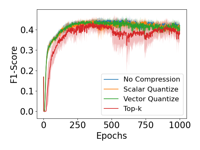
Refer to caption
(a) 222 bits per parameter
Refer to caption
(b) 333 bits per parameter
Refer to caption
(c) 444 bits per parameter
Figure D.1: Test F1subscript𝐹1F_{1}-Score on MIMIC-III dataset. Scalar and vector In these experiments, Q=10𝑄10Q=10 and M=4𝑀4M=4. quantization achieve similar test F1subscript𝐹1F_{1}-Score even when only using 222 bits in quantization. On the other hand, top-k𝑘k sparsification performs worse than the other compressors in the MIMIC-III dataset.

Figure D.1 plots the test F1subscript𝐹1F_{1}-Score for training on the MIMIC-III dataset for different levels of compression. We can see that scalar and vector quantization perform similarly to no compression and improve as the number of bits available increase. We can also see that top-k𝑘k sparsification has high variability on the MIMIC-III dataset and generally performs worse than the other compressors.
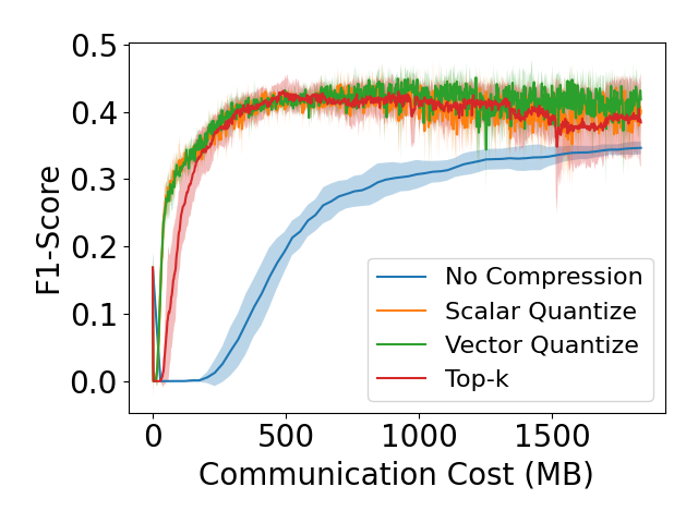
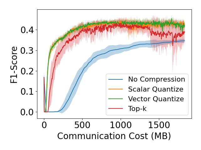
Refer to caption
(a) 222 bits per parameter
Refer to caption
(b) 333 bits per parameter
Refer to caption
(c) 444 bits per parameter
Figure D.2: Test F1subscript𝐹1F_{1}-Score on MIMIC-III dataset plotted by communication cost. In these experiments, Q=10𝑄10Q=10 and M=4𝑀4M=4. We can see that all compressors reach higher F1subscript𝐹1F_{1}-Scores with lower communication cost than no compression. We can see that the standard deviation for each compressor decreases as the number of bits available increases. Top-k𝑘k sparsification generally performs worse than the other compressors on the MIMIC-III-dataset.
Refer to caption
(a) Scalar quantization
Refer to caption
(b) Vector quantization
Refer to caption
(c) Top-k𝑘k sparsification
Figure D.3: Test F1subscript𝐹1F_{1}-Score on MIMIC-III dataset plotted by communication cost. In these experiments, Q=10𝑄10Q=10 and M=4𝑀4M=4. We can see that all compressors reach higher F1subscript𝐹1F_{1}-Scores with lower communication cost than no compression. We can see that the variability for each compressor decreases as the number of bits available increases.

Figures D.2 and D.3 plot the test F1subscript𝐹1F_{1}-Score for training on the MIMIC-III dataset plotted against the communication cost. The plots in Figure D.2 include all compression techniques for a given level of compression, while the plots in Figure D.3 include all levels of compression for a given compression technique. We can see that all compressors reach higher F1subscript𝐹1F_{1}-Scores with lower communication cost than no compression. It is interesting to note that increasing the number of bits per parameter reduces the variability in all compressors.
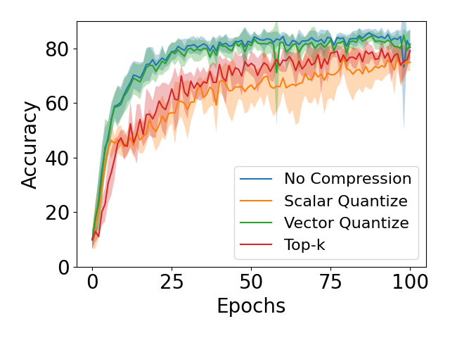
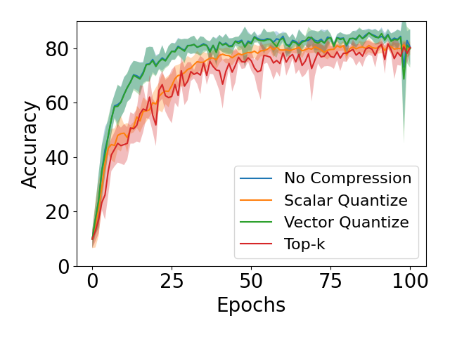
Refer to caption
(a) 222 bits per parameter
Refer to caption
(b) 333 bits per parameter
Refer to caption
(c) 444 bits per parameter
Figure D.4: Test accuracy on ModelNet10 dataset. Vector quantization In these experiments, Q=10𝑄10Q=10 and M=4𝑀4M=4. and top-k𝑘k sparsification perform similarly to no compression, even when only 222 bits are available. Scalar quantization converges to a lower test accuracy, and has high variability on the ModelNet10 dataset.

Figure D.4 plots the test accuracy for training on the ModelNet10 dataset. Vector quantization and top-k𝑘k sparsification perform similarly to no compression, even when only 222 bits are available. We can see that scalar quantization has high variability on the ModelNet10 dataset.
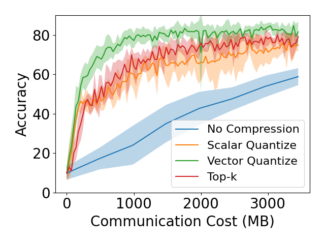
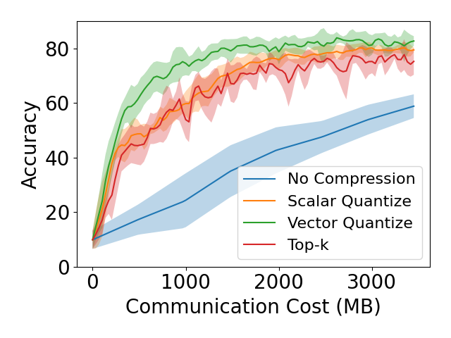
Refer to caption
(a) 222 bits per parameter
Refer to caption
(b) 333 bits per parameter
Refer to caption
(c) 444 bits per parameter
Figure D.5: Test accuracy on ModelNet10 dataset plotted by communication cost. In these experiments, Q=10𝑄10Q=10 and M=4𝑀4M=4. We can see that all compressors reach higher accuracies with lower communication cost than no compression. Scalar quantization generally performs worse than the other compressors on the ModelNet10 dataset.
Refer to caption
(a) Scalar quantization
Refer to caption
(b) Vector quantization
Refer to caption
(c) Top-k𝑘k sparsification
Figure D.6: Test accuracy on ModelNet10 dataset plotted by communication cost. In these experiments, Q=10𝑄10Q=10 and M=4𝑀4M=4. We can see that all compressors reach higher accuracies with lower communication cost than no compression. We can see that when less bits are used in each compressor, higher test accuracies are reached at lower communication costs. Scalar quantization generally performs worse than the other compressors on the ModelNet10 dataset.

Figures D.5 and D.6 plot the test accuracy for training on the ModelNet10 dataset against the communication cost. The plots in Figure D.5 include all compression techniques for a given level of compression, while the plots in Figure D.6 include all levels of compression for a given compression technique. We can see that all compressors reach higher accuracies with lower communication cost than no compression. Scalar quantization generally performs worse than the other compressors on the ModelNet10 dataset. From Figure D.6, we also see that when fewer bits are used in each compressor, higher test accuracies are reached at lower communication costs.
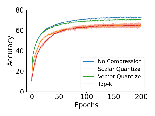
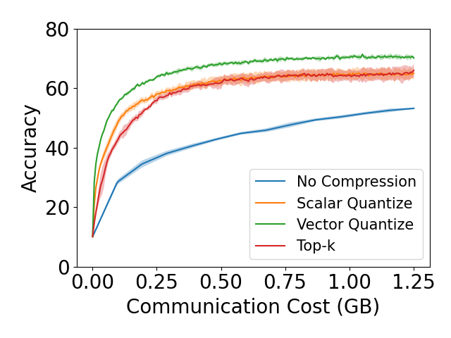
Refer to caption
(a) Plotted by epochs
Refer to caption
(b) Plotted by cost
Refer to caption
(c) Vector quantization
Figure D.7: Test accuracy on CIFAR-10 dataset with the number of parties M=4𝑀4M=4 and number of local iterations Q=10𝑄10Q=10. In the first two plots, the compressors have b=2𝑏2b=2, where b𝑏b is the number of bits used to represent embedding components. In the third plot, b=32𝑏32b=32 indicates there is no compression. The results show vector quantization performs the best our of the compressors, and all compressors show improvement over no compression in terms of communication cost to reach target test accuracies.

In Figure D.7, we plot the test accuracy for the CIFAR-10 dataset. The test accuracy is fairly low compared to typical baseline accuracies, which is expected, as learning object classification from only a quadrant of a 32×32323232\times 32 pixel image is difficult. Figure 7(a) shows the test accuracy plotted by epochs. We can see that vector quantization performs almost as well as no compression in the CIFAR-10 dataset. When plotting by communication cost, seen in Figure 7(b), we can see that vector quantization performs the best, though scalar quantization and top-k𝑘k sparsification show communication savings as well. In Figure 7(c), we plot the test accuracy of C-VFL using vector quantization for different values of b𝑏b, the number of bits to represent compressed values. Similar to previous results, lower b𝑏b tends to improve test accuracy reached with the same amount of communication cost.

D.2 Additional Experiments With ImageNet

We also run C-VFL on ImageNet100 (Deng et al., 2009). ImageNet is a large image dataset for object classification. We use a random subset of 100 classes (ImageNet100) from the ImageNet dataset (about 126126126,000000000 images). We train a set of 444 parties, each storing a different quadrant of every image. Each party trains ResNet18, and the server trains a fully-connected layer. We use a variable step size, that starts at 0.0010.0010.001, and drops to 0.00010.00010.0001 after 505050 epochs. We use a batch size of 256256256 and train for 100100100 epochs.

Refer to caption
(a) Plotted by epochs
Refer to caption
(b) Plotted by cost
Refer to caption
(c) Vector quantization
Figure D.8: Test accuracy on ImageNet-100 dataset with the number of parties M=4𝑀4M=4 and number of local iterations Q=10𝑄10Q=10. In the first two plots, the compressors have b=2𝑏2b=2, where b𝑏b is the number of bits used to represent embedding components. In the third plot, b=32𝑏32b=32 indicates there is no compression. The results show vector quantization performs the best our of the compressors, and all compressors show improvement over no compression in terms of communication cost to reach target test accuracies.

In Figure D.8, we plot the top-555 test accuracy for ImageNet100. Figure 8(a) shows the test accuracy plotted by epochs. We can see that vector quantization performs almost as well as no compression in the ImageNet100 dataset. When plotting by communication cost, seen in Figure 8(b), we can see that vector quantization performs the best, though scalar quantization and top-k𝑘k sparsification show communication savings as well. In Figure 8(c), we plot the test accuracy of C-VFL using vector quantization for different values of b𝑏b, the number of bits to represent compressed values. Similar to previous results, lower b𝑏b tends to improve test accuracy reached with the same amount of communication cost.

D.3 Comparison With Alternative C-VFL Algorithm For Q=1𝑄1Q=1

In C-VFL, the server distributes party embeddings to all parties along with the server model parameters. This allows parties to calculate their partial derivatives for local model updates for multiple local iterations. However, if the number of local iterations Q=1𝑄1Q=1, then a more efficient method of communication is for the server to compute partial derivative updates for the parties (Hu et al., 2019; Ceballos et al., 2020; Romanini et al., 2021), avoiding the need for parties to receive embeddings from other parties. This approach can be applied to C-VFL as well.

1:  Initialize: θm0superscriptsubscript𝜃𝑚0\theta_{m}^{0} for all parties m𝑚m and server model θ00superscriptsubscript𝜃00\theta_{0}^{0}
2:  for t0,,T1𝑡0𝑇1t\leftarrow 0,\ldots,T-1 do
3:     Randomly sample Bt{X,y}superscriptB𝑡Xy\operatorname{\textbf{B}}^{t}\in\{\operatorname{\textbf{X}},\operatorname{\textbf{y}}\}
4:     for m1,,M𝑚1𝑀m\leftarrow 1,\ldots,M in parallel do
5:        Send 𝒞m(hm(θmt;XmBt))subscript𝒞𝑚subscript𝑚superscriptsubscript𝜃𝑚𝑡subscriptsuperscriptXsuperscriptB𝑡𝑚\mathcal{C}_{m}(h_{m}(\theta_{m}^{t};\operatorname{\textbf{X}}^{\operatorname{\textbf{B}}^{t}}_{m})) to server
6:     end for
7:     Φ^t{𝒞0(θ0),𝒞1(h1(θ1t)),,𝒞M(hM(θMt))}superscript^Φ𝑡subscript𝒞0subscript𝜃0subscript𝒞1subscript1superscriptsubscript𝜃1𝑡subscript𝒞𝑀subscript𝑀superscriptsubscript𝜃𝑀𝑡\hat{\Phi}^{t}\leftarrow\{\mathcal{C}_{0}(\theta_{0}),\mathcal{C}_{1}(h_{1}(\theta_{1}^{t})),\ldots,\mathcal{C}_{M}(h_{M}(\theta_{M}^{t}))\}
8:     θ0t+1=θ0tηt0FB(Φ^t;yBt)superscriptsubscript𝜃0𝑡1superscriptsubscript𝜃0𝑡superscript𝜂𝑡subscript0subscript𝐹Bsuperscript^Φ𝑡superscriptysuperscriptB𝑡\theta_{0}^{t+1}=\theta_{0}^{t}-\eta^{t}\nabla_{0}F_{\operatorname{\textbf{B}}}(\hat{\Phi}^{t};\operatorname{\textbf{y}}^{\operatorname{\textbf{B}}^{t}})
9:     Server sends hm(θmt;XmBt)FB(Φ^t;yBt)subscriptsubscript𝑚superscriptsubscript𝜃𝑚𝑡subscriptsuperscriptXsuperscriptB𝑡𝑚subscript𝐹Bsuperscript^Φ𝑡superscriptysuperscriptB𝑡\nabla_{h_{m}(\theta_{m}^{t};\operatorname{\textbf{X}}^{\operatorname{\textbf{B}}^{t}}_{m})}F_{\operatorname{\textbf{B}}}(\hat{\Phi}^{t};\operatorname{\textbf{y}}^{\operatorname{\textbf{B}}^{t}}) to each party m𝑚m
10:     for m1,,M𝑚1𝑀m\leftarrow 1,\ldots,M in parallel do
11:        mFB(Φ^t;yBt)=θmhm(θmt;XmBt)hm(θmt;XmBt)FB(Φ^t;yBt)subscript𝑚subscript𝐹Bsuperscript^Φ𝑡superscriptysuperscriptB𝑡subscriptsubscript𝜃𝑚subscript𝑚superscriptsubscript𝜃𝑚𝑡subscriptsuperscriptXsuperscriptB𝑡𝑚subscriptsubscript𝑚superscriptsubscript𝜃𝑚𝑡subscriptsuperscriptXsuperscriptB𝑡𝑚subscript𝐹Bsuperscript^Φ𝑡superscriptysuperscriptB𝑡\nabla_{m}F_{\operatorname{\textbf{B}}}(\hat{\Phi}^{t};\operatorname{\textbf{y}}^{\operatorname{\textbf{B}}^{t}})=\nabla_{\theta_{m}}h_{m}(\theta_{m}^{t};\operatorname{\textbf{X}}^{\operatorname{\textbf{B}}^{t}}_{m})\nabla_{h_{m}(\theta_{m}^{t};\operatorname{\textbf{X}}^{\operatorname{\textbf{B}}^{t}}_{m})}F_{\operatorname{\textbf{B}}}(\hat{\Phi}^{t};\operatorname{\textbf{y}}^{\operatorname{\textbf{B}}^{t}})
12:        θmt+1=θmtηtmFB(Φ^t;yBt)superscriptsubscript𝜃𝑚𝑡1superscriptsubscript𝜃𝑚𝑡superscript𝜂𝑡subscript𝑚subscript𝐹Bsuperscript^Φ𝑡superscriptysuperscriptB𝑡\theta_{m}^{t+1}=\theta_{m}^{t}-\eta^{t}\nabla_{m}F_{\operatorname{\textbf{B}}}(\hat{\Phi}^{t};\operatorname{\textbf{y}}^{\operatorname{\textbf{B}}^{t}})
13:     end for
14:  end for
Algorithm 2 Compressed Vertical Federated Learning for Q=1𝑄1Q=1

The pseudo-code for this method is presented in Algorithm 2. In this version of C-VFL, parties send their compressed embeddings to the server. The server calculates the loss by feeding the embeddings through the server model. The server calculates the gradient with respect to the loss. The server then sends to each party m𝑚m the partial derivative with respect to its embedding: hm(θmt;XmBt)FB(Φ^t;yBt)subscriptsubscript𝑚superscriptsubscript𝜃𝑚𝑡subscriptsuperscriptXsuperscriptB𝑡𝑚subscript𝐹Bsuperscript^Φ𝑡superscriptysuperscriptB𝑡\nabla_{h_{m}(\theta_{m}^{t};\operatorname{\textbf{X}}^{\operatorname{\textbf{B}}^{t}}_{m})}F_{\operatorname{\textbf{B}}}(\hat{\Phi}^{t};\operatorname{\textbf{y}}^{\operatorname{\textbf{B}}^{t}}). Each party m𝑚m calculates the following partial derivative with respect to its local model parameters:

mFB(Φ^t;yBt)=θmhm(θmt;XmBt)hm(θmt;XmBt)FB(Φ^t;yBt).subscript𝑚subscript𝐹Bsuperscript^Φ𝑡superscriptysuperscriptB𝑡subscriptsubscript𝜃𝑚subscript𝑚superscriptsubscript𝜃𝑚𝑡subscriptsuperscriptXsuperscriptB𝑡𝑚subscriptsubscript𝑚superscriptsubscript𝜃𝑚𝑡subscriptsuperscriptXsuperscriptB𝑡𝑚subscript𝐹Bsuperscript^Φ𝑡superscriptysuperscriptB𝑡\displaystyle\nabla_{m}F_{\operatorname{\textbf{B}}}(\hat{\Phi}^{t};\operatorname{\textbf{y}}^{\operatorname{\textbf{B}}^{t}})=\nabla_{\theta_{m}}h_{m}(\theta_{m}^{t};\operatorname{\textbf{X}}^{\operatorname{\textbf{B}}^{t}}_{m})\nabla_{h_{m}(\theta_{m}^{t};\operatorname{\textbf{X}}^{\operatorname{\textbf{B}}^{t}}_{m})}F_{\operatorname{\textbf{B}}}(\hat{\Phi}^{t};\operatorname{\textbf{y}}^{\operatorname{\textbf{B}}^{t}}). (D.1)

Using this partial derivative, the party updates its local model:

θmt+1=θmtηt0mFB(Φ^mt;yBt0).superscriptsubscript𝜃𝑚𝑡1superscriptsubscript𝜃𝑚𝑡superscript𝜂subscript𝑡0subscript𝑚subscript𝐹Bsuperscriptsubscript^Φ𝑚𝑡superscriptysuperscriptBsubscript𝑡0\displaystyle\theta_{m}^{t+1}=\theta_{m}^{t}-\eta^{t_{0}}\nabla_{m}F_{\operatorname{\textbf{B}}}(\hat{\Phi}_{m}^{t};\operatorname{\textbf{y}}^{\operatorname{\textbf{B}}^{t_{0}}}). (D.2)

Note that this process is mathematically equivalent to C-VFL when Q=1𝑄1Q=1; thus the analysis in Section 4 holds. The communication cost of Algorithm 2 per communication round without compression is O(BmPm)𝑂𝐵subscript𝑚subscript𝑃𝑚O(B\cdot\sum_{m}P_{m}), a reduction in communication compared to the communication cost per round of Algorithm 1: O(M(BmPm+|θ0|))𝑂𝑀𝐵subscript𝑚subscript𝑃𝑚subscript𝜃0O(M\cdot(B\cdot\sum_{m}P_{m}+|\theta_{0}|)). Although Algorithm 2 reduces communication in a given round, it is limited to the case when Q=1𝑄1Q=1. For Q>1𝑄1Q>1, we must use Algorithm 1.

Table D.1: MIMIC-III communication cost to reach a target test F1subscript𝐹1F_{1}-Score of 0.40.40.4. Value shown is the mean of 555 runs, ±plus-or-minus\pm the standard deviation. The first row has no embedding compression, while the second row employs vector quantization on embeddings with b=3𝑏3b=3. For the cases where Q=1𝑄1Q=1, Algorithm 2 is used, and for cases where Q>1𝑄1Q>1, Algorithm 1 is used. In these experiments, the number of clients M=4𝑀4M=4.
Compressor Cost (MB) to Reach Target F1subscript𝐹1F_{1}-Score 0.40.40.4
Q=1𝑄1Q=1 Q=10𝑄10Q=10 Q=25𝑄25Q=25
None b=32𝑏32b=32 4517.59 ±plus-or-minus\pm 465.70 3777.21 ±plus-or-minus\pm 522.43 1536.69 ±plus-or-minus\pm 201.99
Vector b=3𝑏3b=3 433.28 ±plus-or-minus\pm 79.83 330.47 ±plus-or-minus\pm 10.63 125.09 ±plus-or-minus\pm 4.56

We run experiments on the MIMIC-III dataset to compare C-VFL using Algorithm 2 with C-VFL using Algorithm 1 with values of Q>1𝑄1Q>1. We show the results of these experiments in Table D.1. Here, we show the communication cost to reach a target F1subscript𝐹1F_{1}-Score of 0.40.40.4. The results in the column labeled Q=1𝑄1Q=1 are from running Algorithm 2, while all other results are from running Algorithm 1. We include results for the case where C-VFL is run without embedding compression, as well as results for the case where vector quantization with b=3𝑏3b=3 is used to compress embeddings. We can see that for this dataset, values of Q>1𝑄1Q>1 reduce the cost of communication to reach the target F1subscript𝐹1F_{1}-Score. In all cases, Algorithm 1 achieves lower communication cost to reach a target model accuracy than Algorithm 2, despite Algorithm 2 having a lower communication cost per communication round than Algorithm 1. The use of multiple local iterations in Algorithm 1 decreased the number of global rounds required to attain the target accuracy compared to Algorithm 2.