Assessing the Value of Transfer Learning Metrics for RF Domain Adaptation

Abstract.

The use of TL techniques has become common practice in fields such as CV and NLP. Leveraging prior knowledge gained from data with different distributions, TL offers higher performance and reduced training time, but has yet to be fully utilized in applications of ML and DL techniques to applications related to wireless communications, a field loosely termed RFML. This work begins this examination by evaluating the how RF domain changes encourage or prevent the transfer of features learned by CNN-based automatic modulation classifiers. Additionally, we examine existing transferability metrics, LEEP and LogME, as a means to both select source models for RF domain adaptation and predict post-transfer accuracy without further training.

1. Introduction

Following the release of the DARPA RFMLS program in 2017 (Rondeau, 2017), research into the application of ML and DL techniques to wireless communications problems has risen significantly. The field of RFML continues to be the topic of many government research programs and academic conferences including the IARPA SCISRS program (Kolb, 2021) and the DySPAN (Conference, IEEE Communications Society, 2021). As a result, advances in RFML have yielded increased performance and flexibility in applications such as spectrum awareness, cognitive radio, and networking while reducing the need for expert-defined pre-processing and feature extraction techniques (West and O’Shea, 2017).

(a) Traditional Machine Learning

(b) Transfer Learning

Figure 1. In traditional ML (Fig. 1(a)), a new model is trained from random initialization for each domain/task pairing. TL (Fig. 1(b)) utilizes prior knowledge learned on one domain/task, in the form of a pre-trained model, to improve performance on a second domain and/or task. A concrete example for environmental adaptation to SNR is given in blue.

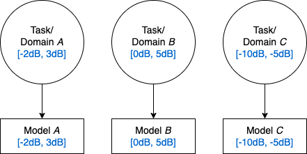
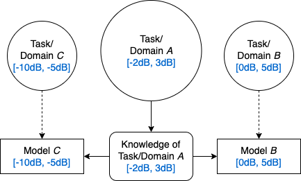
Current state-of-the-art RFML techniques rely upon supervised learning techniques trained from random initialization, and thereby assume the availability of a large corpus of labeled training data (synthetic, captured, or augmented (Clark IV et al., 2020)), which is representative of the anticipated deployed environment. Over time, this assumption inevitably breaks down as a result of changing hardware and channel conditions, and as a consequence, performance degrades significantly (Hauser, 2018; Sankhe et al., 2019). TL techniques can be used to mitigate these performance degradations by using prior knowledge obtained from a source domain and task, in the form of learned representations, to improve performance on a “similar” target domain and task using less data, as depicted in Fig. 1.

Figure 2. A system overview of the RF hardware and channel environment simulated in this work with the parameters/variables ($\alpha[t]$, $\omega[t]$, $\theta[t]$, $\nu[t]$, $\omega_{\Delta}[t]$) that each component of the system has the most significant impact on.

Though TL techniques have demonstrated significant benefits in fields such as CV and NLP (Ruder, 2019), including higher performing models, significantly less training time, and far fewer training samples (Olivas et al., 2009), (Wong and Michaels, 2022) showed that the use of TL in RFML is currently lacking through the construction of an RFML specific TL taxonomy. This work addresses current limitations in understanding how the training domain in particular, characterized by the RF hardware and the channel environment (Wong and Michaels, 2022) depicted in Fig. 2, impacts learned behavior and therefore facilitates or prevents successful transfer.

The contributions of this work are three fold: First, this work systematically evaluates RF domain adaptation performance as a function of several parameters of interest for an AMC use-case (Hauser, 2018): [itemize] @ SNR, which represents a change in the RF channel environment (i.e., an increase/decrease in the additive interference, $\nu[t]$, of the channel) and/or transmitting devices (i.e., an increases/decrease in the magnitude, $\alpha[t]$, of the transmitted signal) and an environment adaptation problem, @ FO, which represents a change in the transmitting and/or receiving devices (i.e., an increase/decrease in $\omega_{\Delta}[t]$ due to hardware imperfections or a lack of synchronization) and a platform adaptation problem, and @ Both SNR and FO, representing a change in both the RF channel environment and the transmitting/receiving devices and an environment platform co-adaptation problem. These three parameter sweeps address each type of RF domain adaptation discussed in the RFML TL taxonomy (Wong and Michaels, 2022), and resulted in the construction of 82 training sets, 82 validation sets, and 82 test sets and the training and evaluation of 4442 models. From these experiments, we identify a number of practical takeaways for how best to perform RF domain adaptation including how changes in SNR and FO impact the difficulty of AMC, an intuitive notion of source/target domain similarity induced by these parameter sweeps, and the impact these have on transfer performance, as well as a comparison of head re-training versus fine-tuning for RF TL.

The second contribution of this work regards how transferability is measured herein. Intuitively, post-transfer top-1 accuracy provides the ground truth measure of transferability, as a measure of performance after transfer learning has occurred through head re-training or fine-tuning of the source model. However, in the scenario where many source models are available for transfer to an alternate domain, evaluating the post-transfer top-1 accuracy for each source model may be too time consuming and computationally expensive. Therefore, in addition to evaluating the transferability of pre-trained source models using post-transfer top-1 accuracy, we examine two existing transferability metrics not known to be used in the RF domain prior to this work: LEEP (Nguyen et al., 2020) and LogME (You et al., 2021). Transferability metrics, such as LEEP and LogME, provide a measure of how well a source model will transfer to a target dataset, and are evaluated without performing transfer learning, using only a single forward pass through the source model. Though LEEP and LogME are designed to be modality independent, we confirm that they are suitable for use in RFML by showing that LEEP and LogME strongly correlate with post-transfer top-1 accuracy, as well as with each other.

Third, we present a method for using transferability metrics such as these to predict post-transfer accuracy, within a confidence interval, and without further training. More specifically, given a labelled target raw IQ dataset and a selection of pre-trained source models, we show that transferability metrics such as LEEP and/or LogME can be used to provide a lower and upper bound on how well each source model will perform once transferred to the target dataset, without performing head re-training or fine-tuning.

In total, this work addresses a number of key research questions, including: [enumerate] @ When and how is RF domain adaptation most successful? – Through exhaustive experimentation, this work provides generalized and practical guidelines for using TL for RF domain adaptation that are intuitive and consistent with the general theory of TL and domain adaptation. @ Can transferability metrics, such as LEEP and LogME, be used to effectively select models for RF domain adaptation? – This work shows that both LEEP and LogME strongly correlate with post-transfer top-1 accuracy in the context of this AMC use-case, and that results are consistent with those shown in the original publications. @ Can transferability metrics, such as LEEP and LogME, predict post-transfer accuracy? – This work presents such an approach, with no additional re-training requirements and confidence intervals provided.

This paper is organized as follows: Section 2 provides requisite background knowledge, and discusses related and prior works in TL for RFML, as well as transferability metrics and transfer accuracy prediction in other modalities such as CV and NLP. In Section 3, each of the key methods and systems used and developed for this work are described in detail, including the simulation environment and dataset creation, the model architecture and training, and the transferability metrics. Section 4 presents experimental results and analysis, addressing the key research questions described above, and the proposed post-transfer accuracy prediction method. Section 5 highlights several directions for future work including extensions of this work performed herein using alternative transferability metrics and captured and/or augmented data, generalizations of this work to inductive TL settings, and developing more robust or RF-specific transferability metrics. Finally, Section 6 offers conclusions about the effectiveness of TL and existing transferability metrics for RFML and next steps for incorporating and extending TL techniques in RFML-based research. A list of the acronyms used in this work is provided in the appendix for reference.

2. Background & Related Work

The recent RFML and TL taxonomies and surveys (Wong and Michaels, 2022; Wong et al., 2021) highlight the limited existing works that successfully use sequential TL techniques for both domain adaptation and inductive transfer including transferring pre-trained models across channel environments (Chen et al., 2019; Pati et al., 2020), across wireless protocols (Kuzdeba et al., 2021; Robinson and Kuzdeba, 2021), and from synthetic data to real data (O’Shea et al., 2018; Dörner et al., 2018; Zheng et al., 2020; Clark et al., 2019), as well as to add or remove output classes (Peng et al., 2020), for tasks such as signal detection, AMC, and SEI. However, outside of observing a lack of direct transfer (Hauser, 2018; Clark IV et al., 2020; Merchant, 2019), little-to-no work has examined what characteristics within RF data facilitate or restrict transfer (Wong and Michaels, 2022). Without such knowledge, TL algorithms for RFML are generally restricted to those borrowed from other modalities, such as CV and NLP. While correlations can be drawn between the vision or language spaces and the RF space, these parallels do not always align, and therefore algorithms designed for CV and NLP may not always be appropriate for use in RFML. In this work, post-transfer top-1 accuracy is paired with existing transferability metrics, LEEP and LogME, to identify how changes in the RF domain impact transferability, and how LEEP and LogME can be of value when performing RF domain adaptation in practice, namely for model selection and post-transfer accuracy prediction.

2.1. Transferability Metrics

As discussed previously, TL techniques use prior knowledge obtained from a source domain/task to improve performance on a similar target domain/task. More specifically, TL techniques aim to further refine a pre-trained source model using a target dataset and specialized training techniques. However, not all pre-trained source models will transfer well to a given target dataset. Though it is generally understood that TL is successful when the source and target domains/tasks are “similar” (Pan and Yang, 2010), this notion of source/target similarity is ill-defined. The goal of a transferability metric is to quantify how well a given pre-trained source model will transfer to a target dataset. While the area of transferability metrics is growing increasingly popular, to our knowledge, no prior works have examined these metrics in the context of RFML. Transferability metrics developed and examined in the context of other modalities can broadly be categorized in one of two ways: those requiring partial re-training and those that do not.

Partial re-training methods such as Taskonomy (Zamir et al., 2018) and Task2Vec (Achille et al., 2019) require some amount of training to occur, whether that be the initial stages of TL, full TL, or the training of an additional probe network, in order to quantify transferability. Partial re-training methods are typically used to identify relationships between source and target tasks and are useful in meta-learning settings, but are not well suited to settings where time and/or computational resources are limited. Though the computational complexity of partial re-training methods varies, it vastly exceeds the computational complexity of methods that do not require any additional training, such as those used in this work.

This work focuses on methods that do not require additional training, which typically use a single forward pass through a pre-trained model to ascertain transferability. Methods such as these are often used to select a pre-trained model from a model library for transfer to a target dataset, a problem known as source model selection. LEEP (Nguyen et al., 2020) and LogME (You et al., 2021) were chosen for this work having outperformed similar metrics such as NCE (Tran et al., 2019) and H-scores (Bao et al., 2019) in CV and NLP-based experiments, and for their modality agnostic design. However, several new transferability metrics developed concurrently with this work also show promise including OTCE (Tan et al., 2021a) and JC-NCE (Tan et al., 2021b), TransRate (Huang et al., 2021), and GBC (Pándy et al., 2021), and may be examined as follow on work.

Related works examine source model ranking or selection procedures (Renggli et al., 2020; Li et al., 2021), which either rank a set of models by transferability or select the model(s) most likely to provide successful transfer. However, source model ranking or selection methods are less flexible than transferability metrics in online or active learning scenarios. More specifically, source model ranking or selection methods are unable to identify how a new source model compares to the already ranked/selected source models without performing the ranking/selection procedure again. Related works also include methods for selecting the best data to use for pre-training (Bhattacharjee et al., 2020) or during the transfer phase (Ruder and Plank, 2017), and approaches to measuring domain, task, and/or dataset similarity (Kashyap et al., 2020).

2.2. Predicting Transfer Accuracy

The problem of predicting transfer accuracy is still an open field. To the best of our knowledge, no prior works have examined predicting transfer accuracy specifically for RFML, but approaches have been developed for other modalities. Most similar to our work is the approach given in (Van Asch and Daelemans, 2010), where the authors showed linear correlation between several domain similarity metrics and transfer accuracy, using statistical inference to derive performance predictions for NLP tools. Similarly, work in (Elsahar and Gallé, 2019) used domain similarity metrics to predict performance drops as a result in domain shift. More recently, (Pogrebnyakov and Shaghaghian, 2021) proposed using a simple MLP to determine how well a source dataset will transfer to a target dataset, again in an NLP setting.

Table 1. Signal types included in this work and generation parameters.

Modulation Name	Parameter Space
BPSK	Symbol Order {2} RRC Pulse Shape Excess Bandwidth {0.35, 0.5} Symbol Overlap $\in$ [3, 5]
QPSK	Symbol Order {4} RRC Pulse Shape Excess Bandwidth {0.35, 0.5} Symbol Overlap $\in$ [3, 5]
PSK8	Symbol Order {8} RRC Pulse Shape Excess Bandwidth {0.35, 0.5} Symbol Overlap $\in$ [3, 5]
PSK16	Symbol Order {16} RRC Pulse Shape Excess Bandwidth {0.35, 0.5} Symbol Overlap $\in$ [3, 5]
OQPSK	Symbol Order {4} RRC Pulse Shape Excess Bandwidth {0.35, 0.5} Symbol Overlap $\in$ [3, 5]
QAM16	Symbol Order {16} RRC Pulse Shape Excess Bandwidth {0.35, 0.5} Symbol Overlap $\in$ [3, 5]
QAM32	Symbol Order {32} RRC Pulse Shape Excess Bandwidth {0.35, 0.5} Symbol Overlap $\in$ [3, 5]
QAM64	Symbol Order {64} RRC Pulse Shape Excess Bandwidth {0.35, 0.5} Symbol Overlap $\in$ [3, 5]
APSK16	Symbol Order {16} RRC Pulse Shape Excess Bandwidth {0.35, 0.5} Symbol Overlap $\in$ [3, 5]

Modulation Name	Parameter Space
APSK32	Symbol Order {32} RRC Pulse Shape Excess Bandwidth {0.35, 0.5} Symbol Overlap $\in$ [3, 5]
FSK5k	Carrier Spacing {5kHz} Rect Phase Shape Symbol Overlap {1}
FSK75k	Carrier Spacing {75kHz} Rect Phase Shape Symbol Overlap {1}
GFSK5k	Carrier Spacing {5kHz} Gaussian Phase Shape Symbol Overlap {2, 3, 4} Beta $\in$ [0.3, 0.5]
GFSK75k	Carrier Spacing {75kHz} Gaussian Phase Shape Symbol Overlap {2, 3, 4 } Beta $\in$ [0.3, 0.5]
MSK	Carrier Spacing {2.5kHz} Rect Phase Shape Symbol Overlap {1}
GMSK	Carrier Spacing {2.5kHz} Gaussian Phase Shape Symbol Overlap {2, 3, 4} Beta $\in$ [0.3, 0.5]
FM-NB	Modulation Index $\in$ [0.05, 0.4]
FM-WB	Modulation Index $\in$ [0.825, 1.88]
AM-DSB	Modulation Index $\in$ [0.5, 0.9]
AM-DSBSC	Modulation Index $\in$ [0.5, 0.9]
AM-LSB	Modulation Index $\in$ [0.5, 0.9]
AM-USB	Modulation Index $\in$ [0.5, 0.9]
AWGN

3. Methodology

(a) The training dataset generation process, repeated to create the validation and test datasets.

(b) The process for model pre-training and TL.

(c) The process for model evaluation and metric calculation.

Figure 3. A system overview of the (a) dataset creation, (b) model pre-training and TL, and (c) model evaluation and transferability metric calculation processes used in this work.

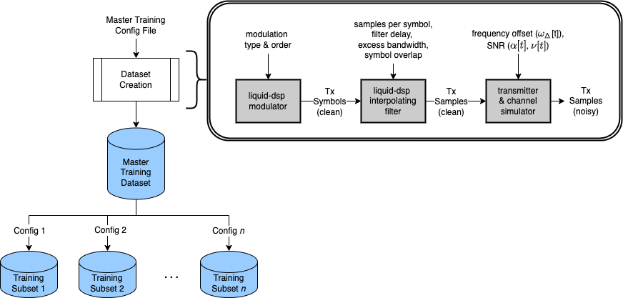
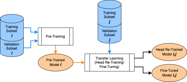
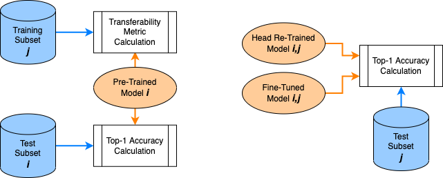
This section presents the experimental setup used in this work, shown in Fig. 3, which includes the data and dataset creation process, the model architecture and training, and the transferability metrics. These three key components and processes are each described in detail in the following subsections.

3.1. Dataset Creation

This work used a custom synthetic dataset generation tool based off the open-source signal processing library liquid-dsp (Gaeddert, 2022), which allowed for full control over the chosen parameters-of-interest, SNR, FO, and modulation type, and ensured accurate labelling of the training, validation, and test data. The dataset creation process, shown in Fig. 3(a), begins with the construction of a large “master” dataset containing all combinations of SNR and FO parameters needed for the experiments performed (Section 3.1.2). Then, for each of the parameter sweeps performed over SNR, FO, and both SNR and FO, subsets of the data were selected from the master dataset using configuration files containing the desired metadata parameters (Sections 3.1.3 - 3.1.5). The master dataset created for this work is publicly available on IEEE DataPort (Wong et al., 2022).

3.1.1. Simulation Environment

All data used in this work was generated using the same noise generation, signal parameters, and signal types as in (Clark et al., 2019). More specifically, in this work, the signal space has been restricted to the 23 signal types shown in Table 1, observed at complex baseband in the form of discrete time-series signals, s[t], where

(1) $$s[t]=\alpha_{\Delta}[t]\cdot\alpha[t]e^{(j\omega[t]+j\theta[t])}\cdot e^{(j\omega_{\Delta}[t]+j\theta_{\Delta}[t])}+\nu[t]\hskip 7.11317pt$$

$\alpha[t]$, $\omega[t]$, and $\theta[t]$ are the magnitude, frequency, and phase of the signal at time $t$, and $\nu[t]$ is the additive interference from the channel. Any values subscripted with a $\Delta$ represent imperfections/offsets caused by the transmitter/receiver and/or synchronization. Without loss of generality, all offsets caused by hardware imperfections or lack of synchronization have been consolidated onto the transmitter during simulation.

Signals are initially synthesized in an AWGN channel environment with unit channel gain, no phase offset, and frequency offset held constant for each observation. Like in (Clark et al., 2019), SNR is defined as

(2) $$\text{SNR}=10\log_{10}\bigg{(}\frac{\sum_{t=1}^{N-1}\lvert s[t]-\nu[t]\rvert^{2}}{\sum_{t=1}^{N-1}\lvert\nu[t]\rvert^{2}}\bigg{)}$$

and, with the exception of the AWGN signal that has a Nyquist rate of 1, all signals have a Nyquist rate of either 0.5 or 0.33 (twice or three times the Nyquist bandwidth).

3.1.2. The Master Dataset

The systematic evaluation of transferability as a function of SNR and FO conducted in this work is possible through the construction of data-subsets with carefully selected metadata parameters from the larger master dataset. The constructed master dataset contains 600000 examples of each the signal types given in Table 1, for a total of 13.8 million examples. For each example, the SNR is selected uniformly at random between [-10dB, 20dB], the FO is selected uniformly at random between [-10%, 10%] of the sample rate, and all further signal generation parameters such as filtering parameters, symbol order, etc. as specified in Table 1. Each example and the associated metadata is saved in SigMF format (Hilburn et al., 2018).

(a) Sweep over SNR.

(b) Sweep over FO.

(c) Sweep over SNR and FO.

Figure 4. The parameter-of-interest range for each data subset selected from the larger master dataset.

3.1.3. SNR Sweep

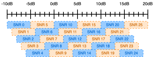
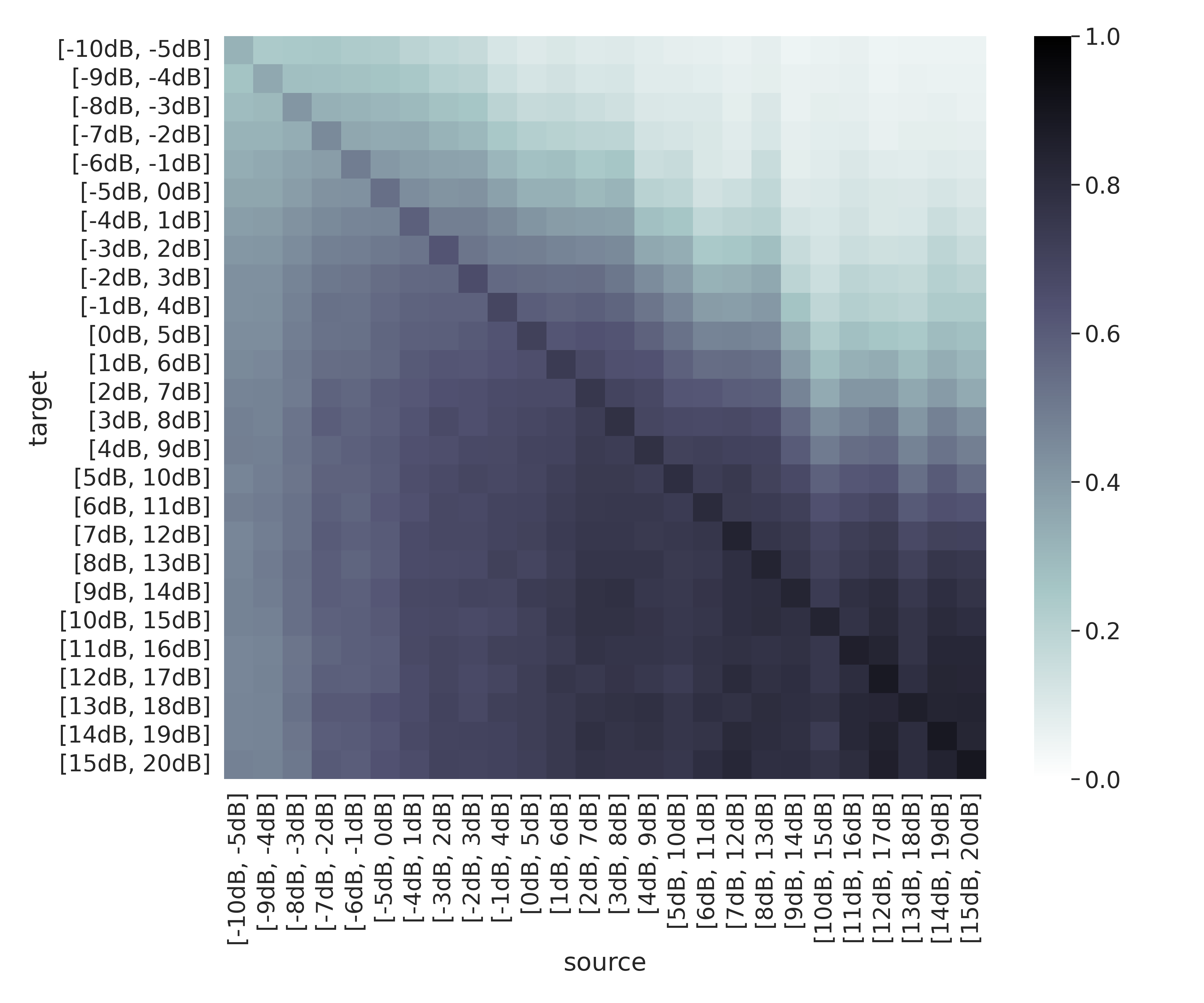
To analyze the impact of SNR alone on transferability, 26 source data-subsets were constructed from the larger master dataset using configuration files, as shown in Fig. 4(a). Each data-subset contains examples with SNR selected uniformly at random from a 5dB range sweeping from -10dB to 20dB in 1dB steps (i.e. [-10dB, -5dB], [-9dB, -4dB], …, [15dB, 20dB]), and for each data-subset in this SNR sweep, FO was selected uniformly at random between [-5%, 5%] of sample rate. This SNR sweep yielded 26 pre-trained source models, each of which was transferred to the remaining 25 target data-subsets (as shown in Fig. 3(b)), yielding 650 models transferred using head re-training and 650 models transferred using fine-tuning.

3.1.4. FO Sweep

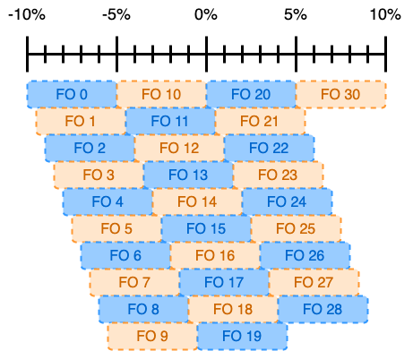
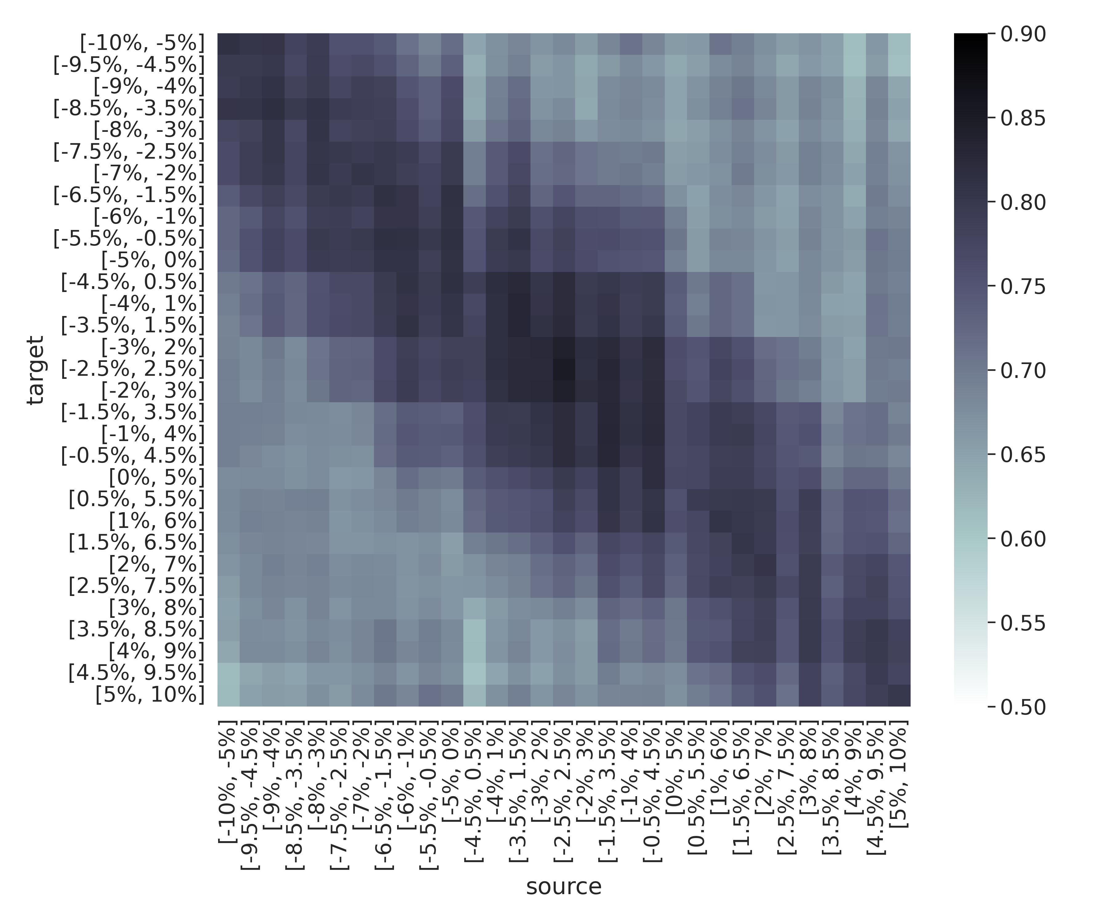
To analyze the impact of FO alone on transferability, 31 source data-subsets were constructed from the larger master dataset (as shown in Fig. 4(b)) containing examples with FO selected uniformly at random from a 5% range sweeping from -10% of sample rate to 10% of sample rate in 0.5% steps (i.e. [-10%, -5%], [-9.5%, -4.5%], …, [5%, 10%]). For each data-subset in this FO sweep, SNR was selected uniformly at random between [0dB, 20dB]. This FO sweep yielded 31 pre-trained source models, each of which was transferred to the remaining 30 target data-subsets (as shown in Fig. 3(b)) yielding 930 models transferred using head re-training, and 930 models transferred using fine-tuning.

3.1.5. SNR $+$ FO Sweep

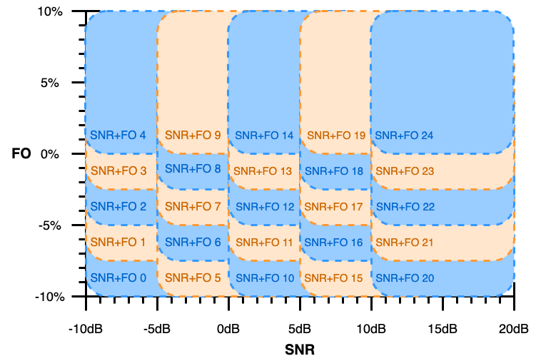
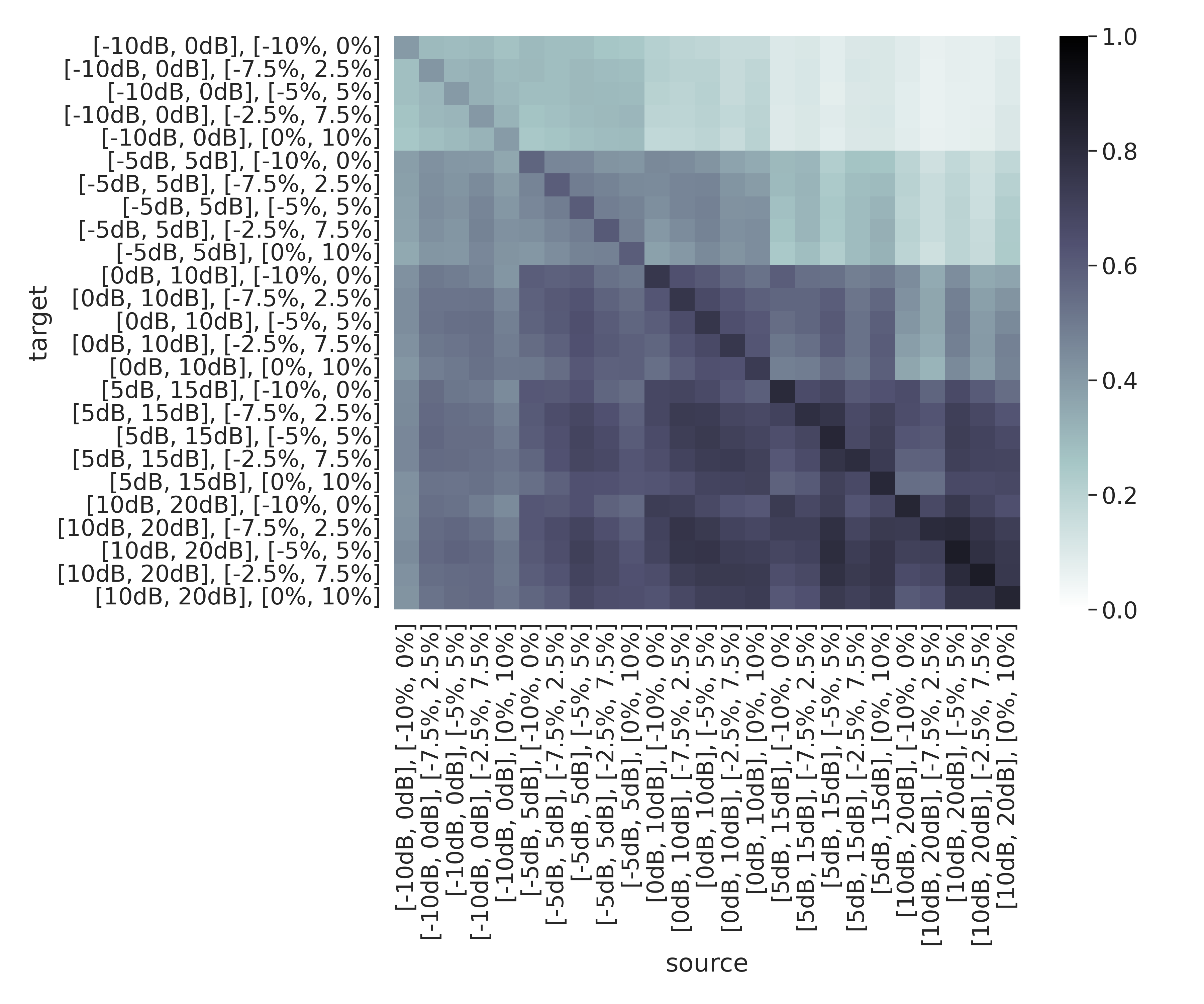
To analyze the impact of both SNR and FO on transferability, 25 source data-subsets were constructed from the larger master dataset (as shown in Fig. 4(c)) containing examples with SNR selected uniformly at random from a 10dB range sweeping from -10dB to 20dB in 5dB steps (i.e. [-10dB, 0dB], [-5dB, 5dB], …, [10dB, 20dB]) and with FO selected uniformly at random from a 10% range sweeping from -10% of sample rate to 10% of sample rate in 2.5% steps (i.e. [-10%, 0%], [-7.5%, 2.5%], …, [0%, 10%]). This SNR and FO sweep yielded 25 pre-trained source models, each of which was transferred to the remaining 24 target data-subsets (as shown in Fig. 3(b)) yielding 600 models transferred using head re-training, and 600 models transferred using fine-tuning.

3.2. Model Architecture and Training

The aim of this work is to use the selected metrics to quantify the ability to transfer the features learned by a single architecture trained across pairwise combinations of source/target datasets with varying (1) SNR, (2) FO, or (3) SNR and FO in order to identify the impact of these parameters-of-interest on transferability. Given the large number of models trained for this work, training time was a primary concern when selecting the model architecture. Therefore, this work uses a simple CNN architecture, shown in Table 2, that is based off of the architectures used in (Clark et al., 2019) and (Wong and McPherson, 2021).

Table 2. Model architecture.

Layer Type	Num Kernels/Nodes	Kernel Size
Input	size = (2, 128)
Conv2d	1500	(1, 7)
ReLU
Conv2d	96	(2, 7)
ReLU
Dropout	rate = 0.5
Flatten
Linear	65
Linear	23
Trainable Parameters: 7434243

The model pre-training and TL process is shown in Fig. 3(b), and represents a standard training pipeline. For pre-training, the training dataset contained 5000 examples per class, and the validation dataset contained 500 examples per class. These dataset sizes are consistent with (Clark et al., 2019) and adequate to achieve consistent convergence. Each model was trained using the Adam optimizer (Kingma and Ba, 2014) and Cross Entropy Loss (pyt, 2021), with the PyTorch default hyper-parameters (Paszke et al., 2019) (a learning rate of 0.001, without weight decay), for a total of 100 epochs. A checkpoint was saved after the epoch with the lowest validation loss, and was reloaded at the conclusion of the 100 epochs. For both head re-training and model fine-tuning, the training dataset contained 500 examples per class, and the validation dataset contained 50 examples per class, representing a smaller sample of available target data. The head re-training and fine-tuning processes both used the Adam optimizer and Cross Entropy Loss as well, with checkpoints saved at the lowest validation loss over 100 epochs. During head re-training, only the final layer of the model was trained, again using the PyTorch default hyper-parameters, while the rest of the model’s parameters were frozen. During fine-tuning, the entire model was trained with a learning rate of 0.0001, an order of magnitude smaller than the PyTorch default of 0.001.

3.3. Transferability Metrics

As previously discussed, while transfer accuracy provides the ground truth measure of transferability, calculating transfer accuracy requires performing sequential learning techniques such as head re-training or fine-tuning to completion, in addition to the labelled target dataset. LEEP (Nguyen et al., 2020) and LogME (You et al., 2021) are existing metrics designed to predicting how well a pre-trained source model will transfer to a labelled target dataset, without performing transfer learning techniques and using only a single forward pass through the pre-trained source model. These metrics in particular were shown to outperform similar metrics, NCE (Tran et al., 2019) and H-scores (Bao et al., 2019), and are designed to be modality agnostic. Therefore, though neither metric is known to have been shown to correlate with transfer accuracy in the context of RFML, the success both metrics showed in CV and NLP applications bodes well for the RF case.

LEEP (Nguyen et al., 2020) can be described as the “average log-likelihood of the expected empirical predictor, a simple classifier that makes prediction[s] based on the expected empirical conditional distribution between source and target labels,” and has been shown to correlate well with transfer accuracy using image data, even when the target datasets are small or imbalanced. The metric is bounded between $(-\infty,0]$, such that values closest to zero indicate best transferability, though the scores tend to be smaller when there are more output classes in the target task. The calculation does not make any assumptions about the similarity of the source/target input data, except that they are the same size. For example, if the source data is raw IQ data of size 2x128, then the target data must also be of size 2x128, but need not be in raw IQ format (i.e. the target data could be in polar format). Therefore, the metric is suitable for estimating transferability when the source and target tasks (output classes) differ. However, the calculation of the metric does require the use of a Softmax output layer, limiting the technique to supervised classifiers.

LogME (You et al., 2021) “estimate[s] the maximum value of label evidence given features extracted by pre-trained models” using a computationally efficient Bayesian algorithm. More specifically, the pre-trained model is used as a feature extractor, and the LogME score is computed using the extracted features and ground truth labels of the target dataset. Like LEEP, the calculation only assumes that the source and target input data are the same size. The metric is bounded between $[-1,1]$, such that values closes to -1 indicate worst transferability and values closest to 1 indicate best transferability. LogME does not require the use of a Softmax output layer, and is therefore appropriate in un-supervised settings, regression settings, and the like. Further, LogME was shown to outperform LEEP in an image classification setting, better correlating with transfer accuracy, and has also shown positive results in an NLP setting.

4. Experimental Results & Analysis

The product of the experiments performed herein is 82 data subsets, each with distinct RF domains, 82 source models trained from random initialization, and 4360 transfer learned models, half transferred using head re-training and the remaining half transferred using fine-tuning. Associated with each of the 4360 transfer learned models is a top-1 accuracy value, a LEEP score, and a LogME score. Given the careful curation of the signal parameters contained within each data subset, as well as the breadth of signal parameters observed, generalized conclusions can be drawn regarding TL performance as function changes in the propagation environment (SNR) and transmitter/receiver hardware (FO). However, it should be noted that further experiments using captured data are required in order to draw more concrete guidelines for using RF TL in the field (Clark IV et al., 2020), and is left for future work. The following subsections present the results obtained from the experiments performed, and discuss how well LEEP and LogME perform in the RF modality, how to use transferability metrics to predict post-transfer performance, as well as some insights and practical takeaways that can be gleaned from the results given including a preliminary understanding of when and how to use TL for RF domain adaptation.

4.1. When and how is RF domain adaptation most successful?

Figure 5. The post-transfer top-1 accuracy for each source/target dataset pair constructed for the sweep over SNR using head re-training to perform domain adaptation. When fine-tuning is used to perform domain adaptation, the same trends are apparent.

Figure 6. The post-transfer top-1 accuracy for each source/target dataset pair constructed for the sweep over FO using head re-training to perform domain adaptation. When fine-tuning is used to perform domain adaptation, the same trends are apparent. Note the scale differs from Figs. 5 and 7.

Figure 7. The post-transfer top-1 accuracy for each source/target dataset pair constructed for the sweep over both SNR and FO using head re-training to perform domain adaptation. When fine-tuning is used to perform domain adaptation, the same trends are apparent.

4.1.1. Impact of Source/Target Domain Similarity and “Difficulty” on Transfer Performance

The heatmaps in Figs. 5-7 show the post-transfer top-1 accuracy achieved with each of the source/target pairs. Note that the post-transfer top-1 accuracy results shown in Figs. 5-7 are from the models that used head re-training to transfer from the source to target domains/datasets. However, the accuracy results from the models that used fine-tuning for transfer show the same trends.

Figs. 5-7 show that highest post-transfer performance is achieved along the diagonal of the heatmap, where the source and target domains are most similar. This behavior is expected, as models trained on similar domains likely learn similar features, and is consistent with the general theory of TL (Pan and Yang, 2010), as well as existing works in modalities outside of RF (Rosenstein et al., 2005). While the notion of domain similarity is ill-defined in general, for the purposes of this work, we are able to say that domains are more similar when the difference between the source and target SNR and/or FO ranges is smaller, as all other data generation parameters are held constant.

Additionally, Figs. 5-7 show that transfer across changes in FO is approximately symmetric, while transfer across changes in SNR are not. This behavior is also expected, and can be attributed to changes in the relative “difficulty” between the source and target domains. More specifically, changing the source/target SNR inherently changes the difficulty of the problem, as performing AMC in lower SNR channel environments is more challenging than performing AMC in high SNR channel environments. Therefore, the source models trained on the lower SNR ranges will transfer to the higher SNR ranges, though may not perform optimally, while the source models trained on the higher SNR ranges will fail to transfer to the lower SNR ranges, as shown in Figs. 5 and 7. In contrast, changing the source/target FO does not make performing AMC any more or less difficult, but may require modifications to the learned features to accommodate this change. Moreover, small changes in FO, $\omega_{\Delta}[t]$, in either the positive and negative direction, are expected to perform similarly. As a result, transfer occurs in either direction off of the diagonal, with best performance closest to the diagonal, as discussed previously.

Practically, these trends indicate that the effectiveness of RF domain adaptation increases as the source and target domains become more similar, and, when applicable, RF domain adaptation is more often successful when transferring from harder to easier domains. For example, transferring from [-5dB, 0dB] to [0dB, 5dB] SNR is likely more effective than transferring from [5dB, 10dB] to [0dB, 5dB] SNR, and transferring from a FO range of [-9%, -4%] of sample rate to [-8%, -3%] of sample rate is likely more effective than transferring from a FO range of [-10%, -5%] of sample rate to [-8%, -3%] of sample rate.

4.1.2. Environment Adaptation vs. Platform Adaptation

Figure 8. The LEEP versus LogME scores for the sweep over SNR, FO, and both SNR and FO. The dashed lines present the linear fit.

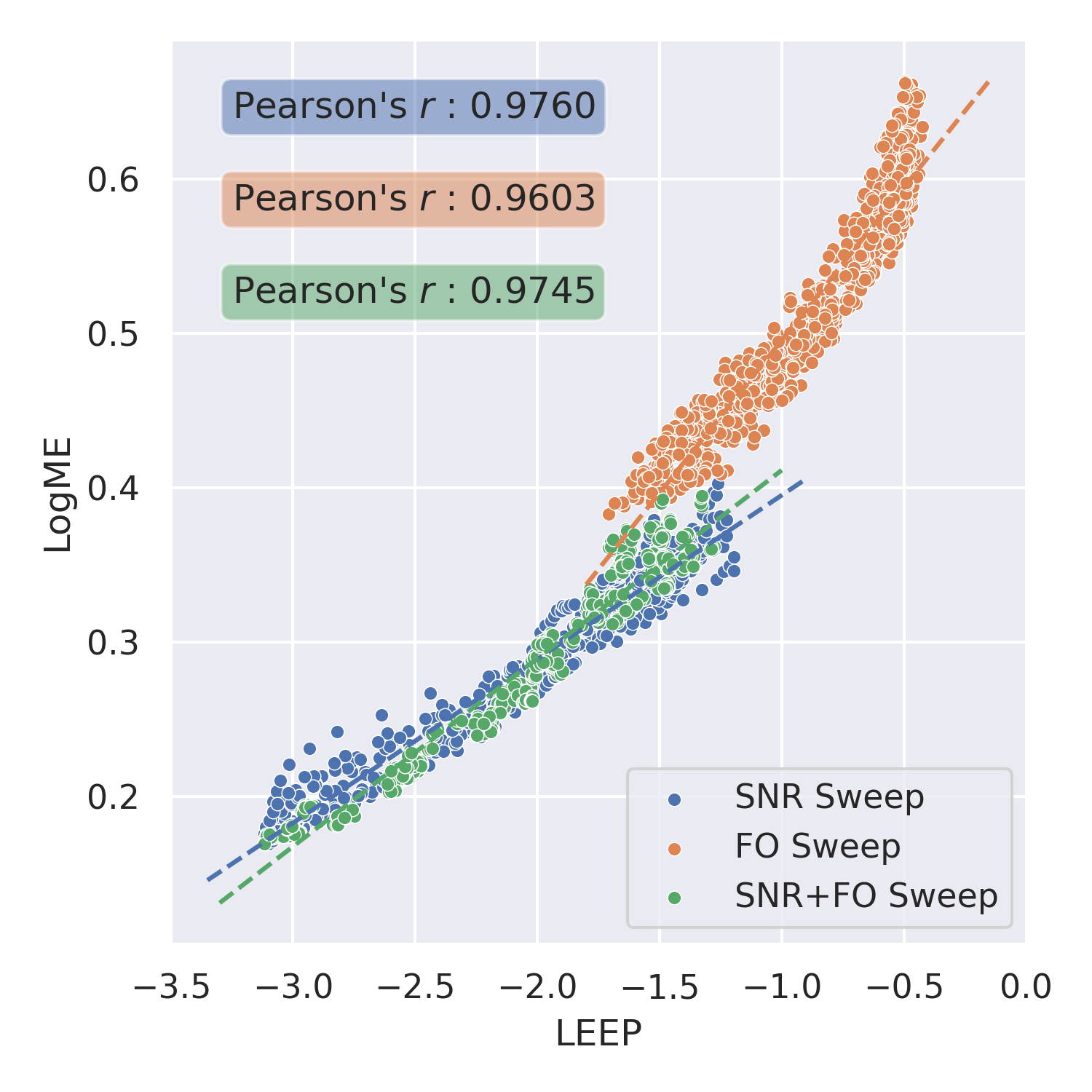
Recalling that the sweep over SNR can be regarded as an environment adaptation experiment and the sweep over FO can be regarded as a platform adaptation experiment, more general conclusions can be drawn regarding the challenges that environment and platform adaptation present. From the discussion in the previous subsection, it follows that changes in FO should be easier to overcome than changes in SNR. That is environment adaptation is more difficult to achieve than platform adaptation, and changes in transmitter/receiver hardware are likely easier to overcome using TL techniques than changes in the channel environment. This trend is indirectly shown through the range of accuracies achieved in Figs. 5-7, which is smaller for the FO sweep than the SNR sweep and SNR $+$ FO sweep, and is more directly shown in Fig. 8. (It should be noted that the scale in Fig. 6 differs from Figs. 5 and 7.) Fig. 8 presents the LogME scores as a function of the LEEP scores for each of the parameter sweeps performed, showing both the LEEP and LogME scores are significantly higher for the FO sweep than the SNR sweep or SNR and FO sweep indicating better transferability. (Of course, this conclusion is dependent upon the results presented in Section 4.2 which show that LEEP and LogME correlate with post-transfer accuracy.) Therefore, in practice, one should consider the similarity of the source/target channel environment before the similarity of the source/target platform, as changes in transmitter/receiver pair are more easily overcome during TL.

4.1.3. Head Re-Training vs. Fine-Tuning

(a)

(b)

Figure 9. The LEEP (a) and LogME (b) scores versus post-transfer top-1 accuracy for the sweep over SNR. The dashed lines present the linear fits for all target domains.

(a)

(b)

Figure 10. The LEEP (a) and LogME (b) scores versus post-transfer top-1 accuracy for the sweep over FO. The dashed lines present the linear fits for all target domains.

(a)

(b)

Figure 11. The LEEP (a) and LogME (b) scores versus post-transfer top-1 accuracy for the sweep over both SNR and FO. The dashed lines present the linear fits for all target domains.

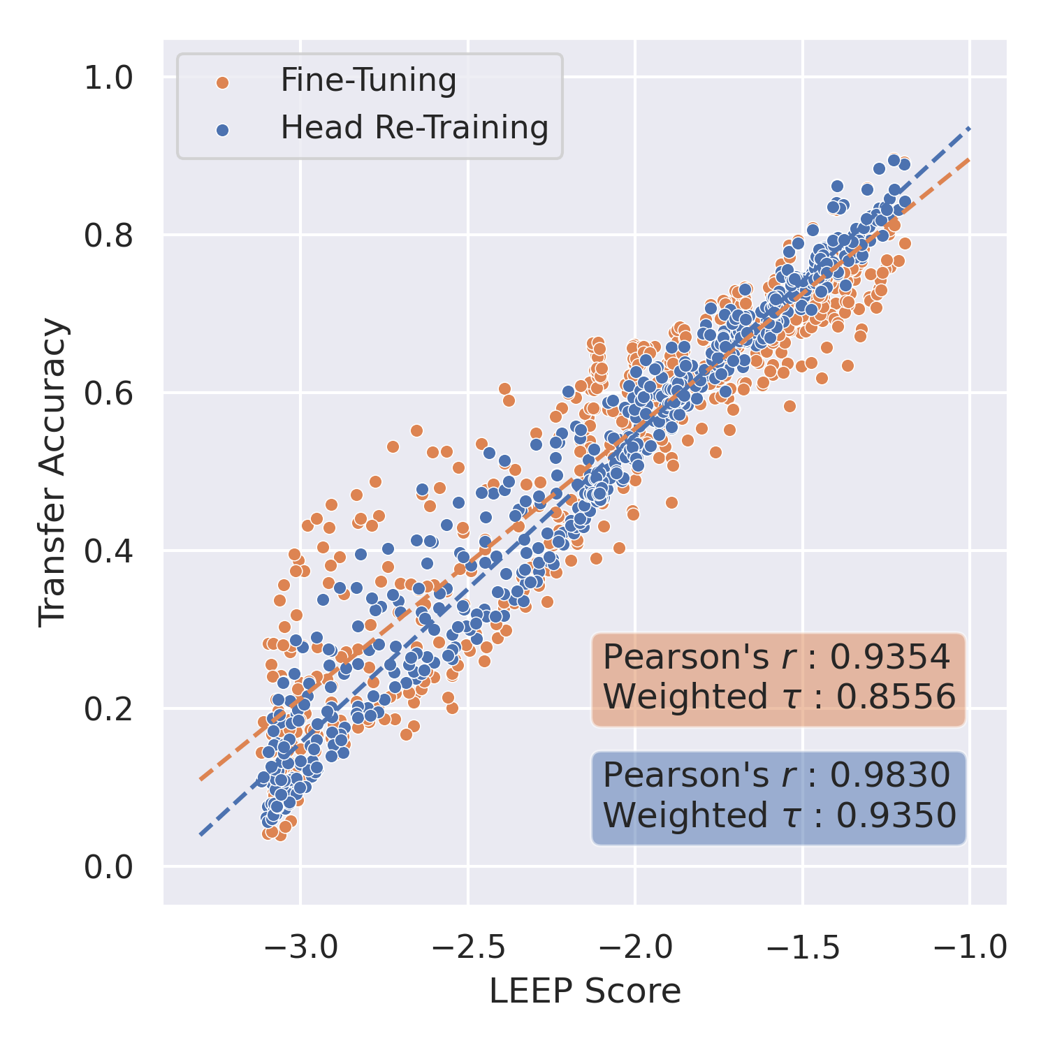
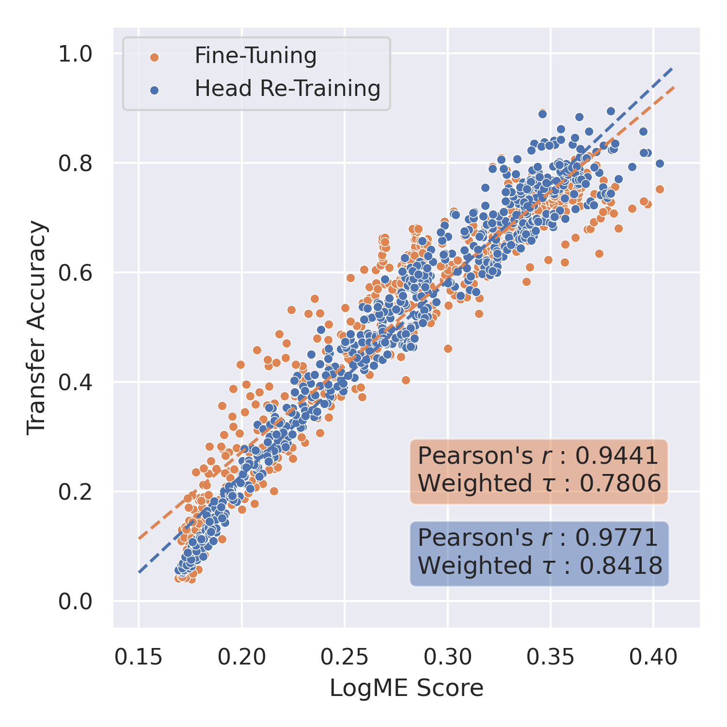
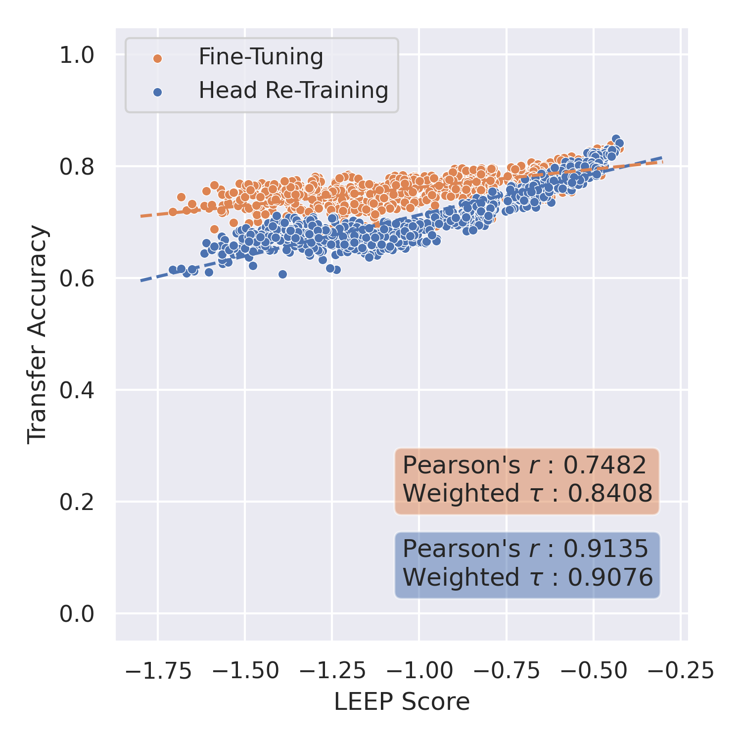
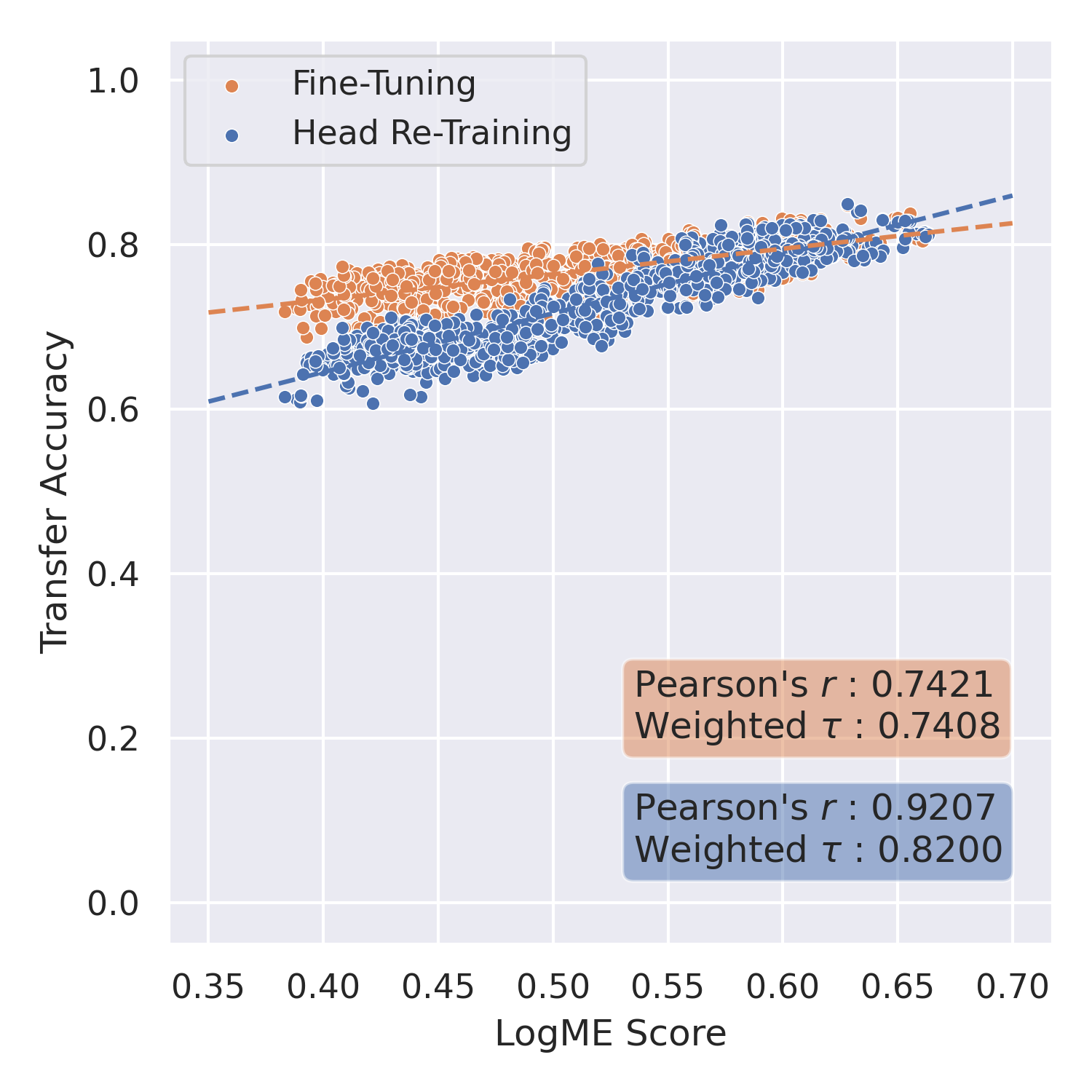
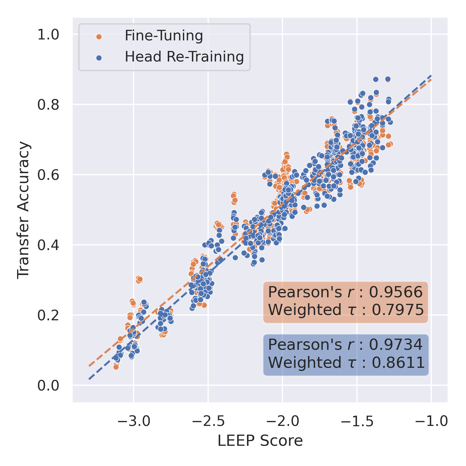
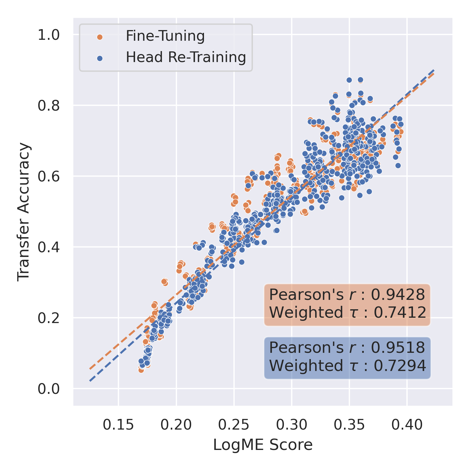
In Figs. 9-11, post-transfer top-1 accuracy is shown as a function of either LEEP or LogME. These figures indicate that when considering post-transfer top-1 accuracy as the sole performance metric, head re-training is as effective as fine-tuning in most settings. The only setting observed herein in which the fine-tuned models markedly outperformed head re-trained models is in the sweep over FO, especially when the LEEP and LogME scores were low. A low LEEP/LogME score indicates a significant change between the source and target domains, in this case a large change in FO. As a result, new features are needed to discern between modulation types, and modifications to the earlier layers of the pre-trained source model, where feature learning occurs, are needed in order to best adapt to the new target domain.

As previously discussed, head re-training is more time efficient and less computationally expensive than fine-tuning, making is a strong case for using head re-training over fine-tuning for RF domain adaptation. The computational complexity of using head re-training versus fine-tuning is architecture and training algorithm dependent, but as an example, for the CNN architecture used in this work and shown in Tab. 2, the number of trainable parameters for head re-training and fine-tuning is 1,518 and 7,434,243 respectively. Finally, the correlation coefficients in Figs. 9-11 show that head re-training is more consistent with LEEP and LogME scores than fine-tuning, leading to the next discussion of whether LEEP and LogME scores can be used to select models for RF domain adaptation.

4.2. Can transferability metrics, such as LEEP and LogME, be used to select models for RF domain adaptation?

When evaluating whether a transferability metric is accurate, the primary consideration is how well the metric reflects or correlates with the performance metric(s) used. Therefore, to identify whether LEEP and/or LogME can be used to select models for RF domain adaptation is to identify how well LEEP and LogME correlate with post-transfer top-1 accuracy. To this end, Figs. 9-11 show LEEP and LogME versus the achieved transfer accuracy for each of the parameter sweeps described in Section 3.1. These figures qualitatively show that both LEEP and LogME correlate well with top-1 accuracy after transfer learning, whether through head re-training or fine-tuning for all domain adaptation settings studied.

To quantify whether or not the metrics are useful, two correlation measures are also examined – the Pearson correlation coefficient (Schober et al., 2018) and the weighted $\tau$ (Kendall, 1938) – specified in the shaded boxes of Figs. 9-11. The Pearson correlation coefficient, or Pearson’s $r$, is a measure of linear correlation between two variables used in a wide variety of works, including the original LEEP paper. However, Pearson’s $r$ makes a number of assumptions about the data, some of which may not be met by this data. Most notably, Pearson’s r assumes that both variables (LEEP/LogME and post-transfer top-1 accuracy, herein) are normally distributed and have a linear relationship. Alternatively, weighted $\tau$, a weighted version of the Kendall rank correlation coefficient (Kendall $\tau$), is used in the original LogME work. Weighted $\tau$ is a measure of correspondence between pairwise rankings, where higher performing/scoring models receive higher weight, and only assumes the variables (LEEP/LogME and post-transfer top-1 accuracy, herein) are continuous. Both Pearson’s $r$ and weighted $\tau$ have a range of $[-1,1]$. These correlation coefficients confirm the results discussed above.

From these figures and metrics it can be concluded that both LEEP and LogME are strong measures for selecting models for RF domain adaptation. However, as alluded to in the previous subsection, head re-training is more consistent with LEEP and LogME scores than fine-tuning, as evidenced by higher correlation coefficients. Therefore, when using LEEP or LogME for model selection, using head re-training as a TL method would be more reliable than using fine-tuning. In contrast, fine-tuning, while less reliable than head re-training when used in conjunction with LEEP or LogME for model selection, offers potential for small performance gains over head re-training. In practice, this indicates that unless top performance is of more value than reliability, head re-training should be used for TL when using LEEP or LogME for model selection. In the setting where model accuracy is of the utmost importance, it may be advantageous to try both head re-training and fine-tuning.

It should also be noted that the results shown in Figs. 9-11 are consistent with the results presented in the original LEEP and LogME publications where the metrics were tested in CV and NLP settings, supporting the claim that these metrics are truly modality agnostic. Therefore, other modality agnostic metrics seem likely to perform well in RFML settings as well, and may be examined as follow on work.

4.3. How can LEEP/LogME be used to predict post-transfer accuracy?

Having confirmed that LEEP and LogME can be used to select models for RF domain adaptation, what follows is an approach to not only select models for RF domain adaptation, but also to predict the post-transfer top-1 accuracy without any further training. The approach is time and resource intensive to initialize, but once initialized, is fast and relatively inexpensive to compute and shows the predictive capabilities of these metrics.

Given $n$ known domains and assuming a single model architecture, to initialize the approach: [enumerate] @ Run baseline simulations for all $n$ known domains including pre-training source models on all domains, and using head re-training and/or fine-tuning to transfer each source model to the remaining known domains @ Compute LEEP/LogME scores using all pre-trained source models and the remaining known domains. @ Compute post-transfer top-1 accuracy for all transfer-learned models, constructing datapoints like those displayed in Figs. 9-11. @ Fit a function of the desired form (i.e. linear, logarithmic, etc.) to the LEEP/LogME scores and post-transfer top-1 accuracies. For example, a linear fit of the form $y=\beta_{0}x+\beta_{1}$ is shown in Figs. 9-11 such that $x$ is the transferability score and $y$ is the post-transfer top-1 accuracy. @ Compute the margin of error by first calculating the mean difference between the true post-transfer top-1 accuracy and the predicted post-transfer top-1 accuracy (using the linear fit), and then multiplying this mean by the appropriate z-score(s) for the desired confidence interval(s) (Hazra, 2017).

Then, during deployment, given a new labelled target dataset: [enumerate] @ Compute LEEP/LogME scores for all pre-trained source models and new target dataset. @ Select the pre-trained source model yielding the highest LEEP/LogME score for TL. @ Use the fitted linear function to estimate post-transfer accuracy, given the highest LEEP/LogME score, and add/subtract the margin of error to construct the confidence interval. Optionally, after transferring to the new labelled target dataset, add this dataset to the list of known domains, and update the linear fit and margin of error, as needed.

Figure 12. The error in the predicted post-transfer accuracy using a linear fit to the LEEP scores (x-axis) and LogME scores (y-axis) for the sweep over SNR.

Figure 13. The error in the predicted post-transfer accuracy using a linear fit to the LEEP scores (x-axis) and LogME scores (y-axis) for the sweep over FO. Note the change in scale compared to Figs. 12 and 14.

Figure 14. The error in the predicted post-transfer accuracy using a linear fit to the LEEP scores (x-axis) and LogME scores (y-axis) for the sweep over both SNR and FO.

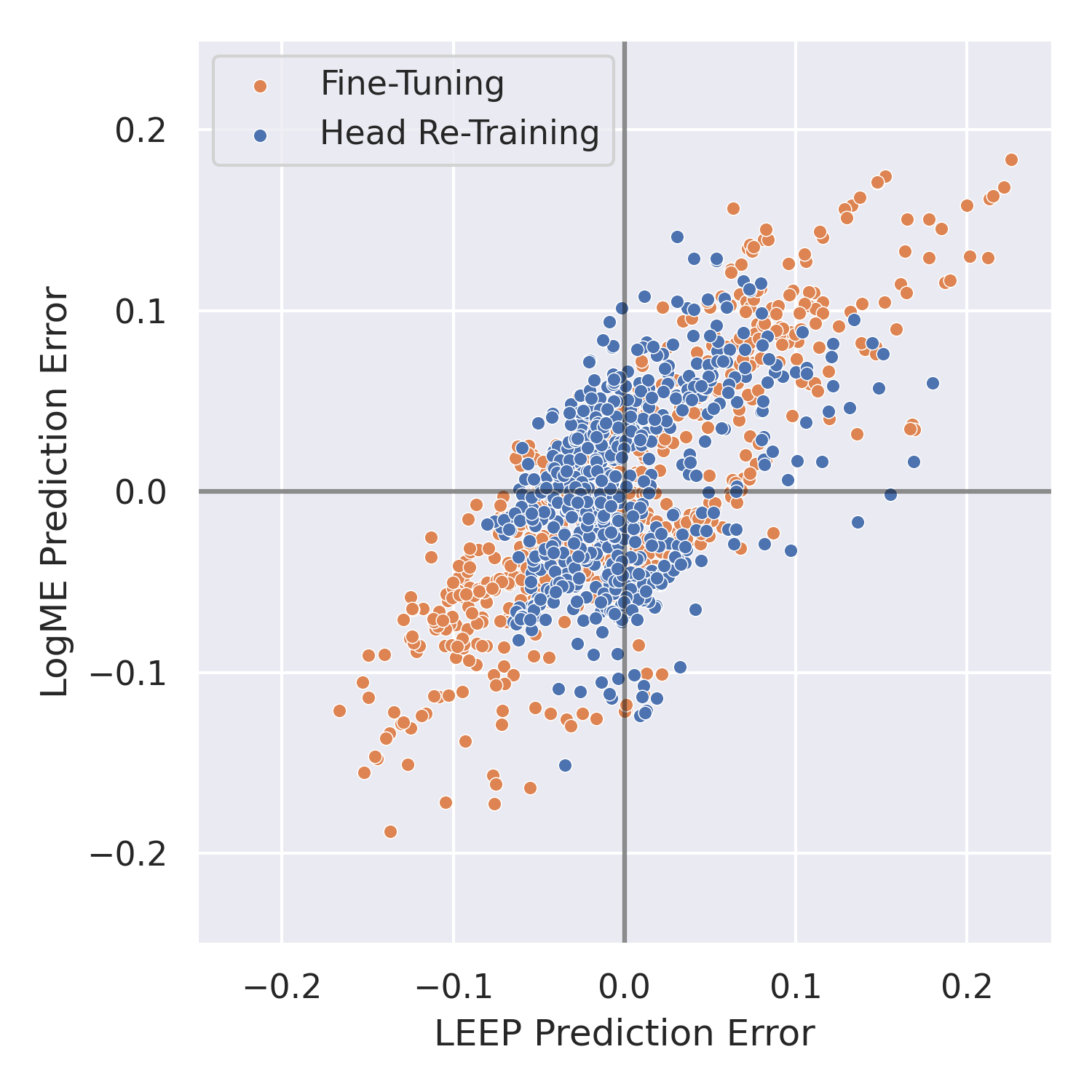
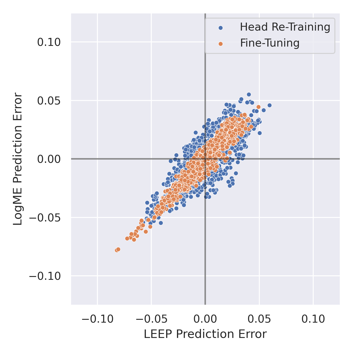
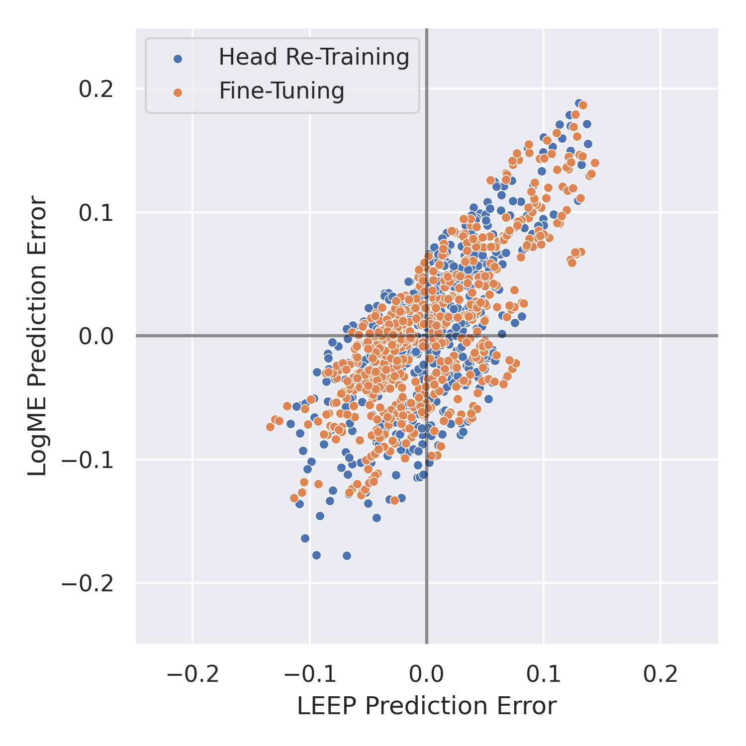
The error in the predicted post-transfer accuracy using the proposed method is shown in Figs. 12-14. These plots show that not only are LEEP/LogME highly correlated with post-transfer top-1 accuracy (as shown in Figs. 9-11), but the error in the predicted post-transfer top-1 accuracy using a linear fit to the LEEP and LogME scores respectively is also highly correlated. More specifically, when the proposed method constructed using LEEP predicts a lower/higher post-transfer accuracy than ground truth, the proposed method constructed using LogME will do the same with the frequencies shown in Tab. 3. This indicates that these scores could be combined to create a more robust transferability metric and more robust post-transfer accuracy prediction with relative ease, which is left for future work.

Table 3. The frequency with which the proposed method constructed using LEEP and LogME agree in over/under predicting post-transfer accuracy.

	SNR Sweep	FO Sweep	SNR + FO Sweep
Head Re-Training	0.6175	0.7856	0.7258
Fine-Tuning	0.7496	0.8803	0.7468

5. Future Work

As previously mentioned, several new transferability metrics were developed concurrently with this work, and are suitable as replacements for LEEP and LogME in any of the above experiments. Therefore, the first direction for future work is replicating this work using alternative metrics such as OTCE (Tan et al., 2021a), JC-NCE (Tan et al., 2021b), TransRate (Huang et al., 2021), and GBC (Pándy et al., 2021), to identify if these metrics are also suitable for use in the context of RFML and if these metrics might outperform those used herein. Given that this work supports the claim that LEEP and LogME are modality agnostic, it seems likely that additional transferability metrics that are also modality agnostic by design will also follow this trend. Additionally, the concept of transferability metrics and the experiments performed herein should be extended to inductive TL settings including multi-task learning and sequential learning settings in which the source and target tasks differ (i.e. adding/removing output classes), as this work only considered RF domain adaptation.

Another direction for future work is the development of new transferability metrics that are more robust than LEEP or LogME alone or are RFML-specific. Most apparently, results discussed previously in Section 4.3 indicate that LEEP and LogME could be combined to create a more robust transferability metric and more robust post-transfer accuracy prediction with relative ease. However, while modality agnostic metrics such as LEEP and LogME are shown herein to be suitable for use in RFML, a transferability metric purpose-built for the RF space would likely be more widely accepted amongst traditional RF engineers (Wong et al., 2021).

With or without the use of transferability metrics, this work provides generalized conclusions about how best to use TL in the context of RFML. Provided future verification and refinement of these results and guidelines using captured and augmented data (Clark IV et al., 2020), this work can be used in future RFML systems to construct the highest performing models for a given target domain when data is limited. More specifically, these guidelines begin a discussion regarding how best to continually update RFML models once deployed, in an online or incremental fashion, to overcome the highly fluid nature of modern communication systems (Wong et al., 2021).

6. Conclusion

TL has yielded tremendous performance benefits in CV and NLP, and as a result, TL is all but commonplace in these fields. However, the benefits of TL have yet to be fully demonstrated and integrated in RFML. To begin to address this deficit, this work systematically evaluated RF domain adaptation performance as a function of several parameters-of-interest, including SNR and FO, using post-transfer top-1 accuracy and existing transferability metrics, LEEP and LogME. This work demonstrated that LEEP and LogME correlate well with post-transfer accuracy, and can therefore be used for model selection successfully in the context of RF domain adaptation. Further, an approach was presented for predicting post-transfer accuracy using these metrics, within a confidence interval, and without further training.

Through this exhaustive study, a number of guidelines have been identified for when and how to use TL for RF domain adaptation successfully. More specifically, results indicate: [itemize] @ Using source models trained on the most similar domain to the target yields highest performance @ Transferring from a more challenging domain than the target, is preferred to transferring from an easier domain @ Selecting source models based on this similarity of the source/target channel environment is more important than the similarity of the source/target platform(s) @ Head re-training is more reliable, faster, and less computationally expensive than fine-tuning for RF domain adaptation @ TL via both head re-training and fine-tuning should be attempted, when top performance is of greater value than time and/or computational efficiency These takeaways can be used in future RFML systems to construct higher performing models when limited data is available, and can be used to develop to online and active RFML approaches, a critical need for practical and deployable RFML.

References

- (1)
- pyt (2021) 2021. Cross Entropy Loss. https://pytorch.org/docs/stable/generated/torch.nn.CrossEntropyLoss.html
- Achille et al. (2019) Alessandro Achille, Michael Lam, Rahul Tewari, Avinash Ravichandran, Subhransu Maji, Charless C Fowlkes, Stefano Soatto, and Pietro Perona. 2019. Task2Vec: Task embedding for meta-learning. In Proceedings of the IEEE/CVF International Conference on Computer Vision. 6430–6439.
- Bao et al. (2019) Yajie Bao, Yang Li, Shao-Lun Huang, Lin Zhang, Lizhong Zheng, Amir Zamir, and Leonidas Guibas. 2019. An Information-Theoretic Approach to Transferability in Task Transfer Learning. In 2019 IEEE International Conference on Image Processing (ICIP). 2309–2313. https://doi.org/10.1109/ICIP.2019.8803726
- Bhattacharjee et al. (2020) Bishwaranjan Bhattacharjee, John R Kender, Matthew Hill, Parijat Dube, Siyu Huo, Michael R Glass, Brian Belgodere, Sharath Pankanti, Noel Codella, and Patrick Watson. 2020. P2L: Predicting transfer learning for images and semantic relations. In Proceedings of the IEEE/CVF Conference on Computer Vision and Pattern Recognition Workshops. 760–761.
- Chen et al. (2019) S. Chen, S. Zheng, L. Yang, and X. Yang. 2019. Deep Learning for Large-Scale Real-World ACARS and ADS-B Radio Signal Classification. IEEE Access 7 (2019), 89256–89264. https://doi.org/10.1109/ACCESS.2019.2925569
- Clark et al. (2019) Bill Clark, Zach Leffke, Chris Headley, and Alan Michaels. 2019. Cyborg Phase II Final Report. Technical Report. Ted and Karyn Hume Center for National Security and Technology.
- Clark et al. (2019) W. H. Clark, V. Arndorfer, B. Tamir, D. Kim, C. Vives, H. Morris, L. Wong, and W. C. Headley. 2019. Developing RFML Intuition: An Automatic Modulation Classification Architecture Case Study. In 2019 IEEE Military Comm. Conference (MILCOM). 292–298. https://doi.org/10.1109/MILCOM47813.2019.9020949
- Clark IV et al. (2020) William H Clark IV, Steven Hauser, William C Headley, and Alan J Michaels. 2020. Training data augmentation for deep learning radio frequency systems. The Journal of Defense Modeling and Simulation (2020).
- Conference, IEEE Communications Society (2021) Conference, IEEE Communications Society. 2021. DySPAN 2021: 2020 IEEE International Symposium on Dynamic Spectrum Access Networks, 13–15 December 2021.
- Dörner et al. (2018) S. Dörner, S. Cammerer, J. Hoydis, and S. t. Brink. 2018. Deep Learning Based Communication Over the Air. IEEE Journal of Selected Topics in Signal Processing 12, 1 (2018), 132–143. https://doi.org/10.1109/JSTSP.2017.2784180
- Elsahar and Gallé (2019) Hady Elsahar and Matthias Gallé. 2019. To annotate or not? Predicting performance drop under domain shift. In Proceedings of the 2019 Conference on Empirical Methods in Natural Language Processing and the 9th International Joint Conference on Natural Language Processing (EMNLP-IJCNLP). 2163–2173.
- Gaeddert (2022) Joseph Gaeddert. 2022. liquid-dsp. https://github.com/jgaeddert/liquid-dsp
- Hauser (2018) Steven Charles Hauser. 2018. Real-World Considerations for Deep Learning in Spectrum Sensing. Master’s thesis. Virginia Tech.
- Hazra (2017) Avijit Hazra. 2017. Using the confidence interval confidently. Journal of thoracic disease 9, 10 (2017), 4125.
- Hilburn et al. (2018) Ben Hilburn, Nathan West, Tim O’Shea, and Tamoghna Roy. 2018. SigMF: the signal metadata format. In Proceedings of the GNU Radio Conference, Vol. 3.
- Huang et al. (2021) Long-Kai Huang, Ying Wei, Yu Rong, Qiang Yang, and Junzhou Huang. 2021. Frustratingly Easy Transferability Estimation. arXiv preprint arXiv:2106.09362 (2021).
- Kashyap et al. (2020) Abhinav Ramesh Kashyap, Devamanyu Hazarika, Min-Yen Kan, and Roger Zimmermann. 2020. Domain divergences: a survey and empirical analysis. arXiv preprint arXiv:2010.12198 (2020).
- Kendall (1938) Maurice G Kendall. 1938. A new measure of rank correlation. Biometrika 30, 1/2 (1938), 81–93.
- Kingma and Ba (2014) Diederik P Kingma and Jimmy Ba. 2014. Adam: A method for stochastic optimization. arXiv preprint arXiv:1412.6980 (2014).
- Kolb (2021) Paul Kolb. 2021. Securing Compartmented Information with Smart Radio Systems (SCISRS). https://www.iarpa.gov/index.php/research-programs/scisrs
- Kuzdeba et al. (2021) Scott Kuzdeba, Josh Robinson, and Joseph Carmack. 2021. Transfer Learning with Radio Frequency Signals. In 2021 IEEE 18th Annual Consumer Communications Networking Conference (CCNC). 1–9. https://doi.org/10.1109/CCNC49032.2021.9369550
- Li et al. (2021) Yandong Li, Xuhui Jia, Ruoxin Sang, Yukun Zhu, Bradley Green, Liqiang Wang, and Boqing Gong. 2021. Ranking neural checkpoints. In Proceedings of the IEEE/CVF Conference on Computer Vision and Pattern Recognition. 2663–2673.
- Merchant (2019) Kevin Merchant. 2019. Deep Neural Networks for Radio Frequency Fingerprinting. Ph. D. Dissertation.
- Nguyen et al. (2020) Cuong Nguyen, Tal Hassner, Matthias Seeger, and Cedric Archambeau. 2020. LEEP: A new measure to evaluate transferability of learned representations. In International Conference on Machine Learning. PMLR, 7294–7305.
- Olivas et al. (2009) Emilio Soria Olivas, Jos David Mart Guerrero, Marcelino Martinez-Sober, Jose Rafael Magdalena-Benedito, L Serrano, et al. 2009. Handbook of research on machine learning applications and trends: Algorithms, methods, and techniques. IGI Global.
- O’Shea et al. (2018) T. J. O’Shea, T. Roy, and T. C. Clancy. 2018. Over-the-Air Deep Learning Based Radio Signal Classification. IEEE Journal of Selected Topics in Signal Processing 12, 1 (2018), 168–179. https://doi.org/10.1109/JSTSP.2018.2797022
- Pan and Yang (2010) S. J. Pan and Q. Yang. 2010. A Survey on Transfer Learning. IEEE Trans. on Knowledge and Data Eng. 22, 10 (2010), 1345–1359. https://doi.org/10.1109/TKDE.2009.191
- Pándy et al. (2021) Michal Pándy, Andrea Agostinelli, Jasper Uijlings, Vittorio Ferrari, and Thomas Mensink. 2021. Transferability Estimation using Bhattacharyya Class Separability. arXiv preprint arXiv:2111.12780 (2021).
- Paszke et al. (2019) Adam Paszke, Sam Gross, Francisco Massa, Adam Lerer, James Bradbury, Gregory Chanan, Trevor Killeen, Zeming Lin, Natalia Gimelshein, Luca Antiga, et al. 2019. PyTorch: An imperative style, high-performance deep learning library. Advances in neural information processing systems 32 (2019), 8026–8037.
- Pati et al. (2020) B. M. Pati, M. Kaneko, and A. Taparugssanagorn. 2020. A Deep Convolutional Neural Network Based Transfer Learning Method for Non-Cooperative Spectrum Sensing. IEEE Access 8 (2020), 164529–164545. https://doi.org/10.1109/ACCESS.2020.3022513
- Peng et al. (2020) Q. Peng, A. Gilman, N. Vasconcelos, P. C. Cosman, and L. B. Milstein. 2020. Robust Deep Sensing Through Transfer Learning in Cognitive Radio. IEEE Wireless Comm. Letters 9, 1 (2020), 38–41. https://doi.org/10.1109/LWC.2019.2940579
- Pogrebnyakov and Shaghaghian (2021) Nicolai Pogrebnyakov and Shohreh Shaghaghian. 2021. Predicting the Success of Domain Adaptation in Text Similarity. arXiv preprint arXiv:2106.04641 (2021).
- Renggli et al. (2020) Cedric Renggli, André Susano Pinto, Luka Rimanic, Joan Puigcerver, Carlos Riquelme, Ce Zhang, and Mario Lucic. 2020. Which model to transfer? Finding the needle in the growing haystack. arXiv preprint arXiv:2010.06402 (2020).
- Robinson and Kuzdeba (2021) Josh Robinson and Scott Kuzdeba. 2021. RiftNet: Radio Frequency Classification for Large Populations. In 2021 IEEE 18th Annual Consumer Communications Networking Conference (CCNC). 1–6. https://doi.org/10.1109/CCNC49032.2021.9369455
- Rondeau (2017) Tom Rondeau. 2017. Radio Frequency Machine Learning Systems (RFMLS). https://www.darpa.mil/program/radio-frequency-machine-learning-systems.
- Rosenstein et al. (2005) Michael T Rosenstein, Zvika Marx, Leslie Pack Kaelbling, and Thomas G Dietterich. 2005. To transfer or not to transfer. In NIPS 2005 workshop on transfer learning, Vol. 898. 1–4.
- Ruder (2019) Sebastian Ruder. 2019. Neural transfer learning for natural language processing. Ph. D. Dissertation. NUI Galway.
- Ruder and Plank (2017) Sebastian Ruder and Barbara Plank. 2017. Learning to select data for transfer learning with bayesian optimization. arXiv preprint arXiv:1707.05246 (2017).
- Sankhe et al. (2019) Kunal Sankhe, Mauro Belgiovine, Fan Zhou, Shamnaz Riyaz, Stratis Ioannidis, and Kaushik Chowdhury. 2019. ORACLE: Optimized Radio Classification through Convolutional Neural Networks. In IEEE INFOCOM 2019-IEEE Conference on Computer Communications. IEEE, 370–378.
- Schober et al. (2018) Patrick Schober, Christa Boer, and Lothar A Schwarte. 2018. Correlation coefficients: appropriate use and interpretation. Anesthesia & Analgesia 126, 5 (2018), 1763–1768.
- Tan et al. (2021a) Yang Tan, Yang Li, and Shao-Lun Huang. 2021a. OTCE: A Transferability Metric for Cross-Domain Cross-Task Representations. In Proceedings of the IEEE/CVF Conference on Computer Vision and Pattern Recognition. 15779–15788.
- Tan et al. (2021b) Yang Tan, Yang Li, and Shao-Lun Huang. 2021b. Practical Transferability Estimation for Image Classification Tasks. arXiv preprint arXiv:2106.10479 (2021).
- Tran et al. (2019) Anh T Tran, Cuong V Nguyen, and Tal Hassner. 2019. Transferability and hardness of supervised classification tasks. In Proceedings of the IEEE/CVF International Conference on Computer Vision. 1395–1405.
- Van Asch and Daelemans (2010) Vincent Van Asch and Walter Daelemans. 2010. Using domain similarity for performance estimation. In Proceedings of the 2010 Workshop on Domain Adaptation for Natural Language Processing. 31–36.
- West and O’Shea (2017) N. E. West and T. O’Shea. 2017. Deep architectures for modulation recognition. In 2017 IEEE Int. Symp. on Dynamic Spectrum Access Networks (DySPAN). 1–6.
- Wong et al. (2022) Lauren Wong, Sean McPherson, and Alan Michaels. 2022. Transfer Learning for RF Domain Adaptation – Synthetic Dataset. https://doi.org/10.21227/42v8-pj22
- Wong et al. (2021) Lauren J. Wong, William H. Clark, Bryse Flowers, R. Michael Buehrer, William C. Headley, and Alan J. Michaels. 2021. An RFML Ecosystem: Considerations for the Application of Deep Learning to Spectrum Situational Awareness. IEEE Open Journal of the Communications Society 2 (2021), 2243–2264. https://doi.org/10.1109/OJCOMS.2021.3112939
- Wong and McPherson (2021) Lauren J. Wong and Sean McPherson. 2021. Explainable Neural Network-based Modulation Classification via Concept Bottleneck Models. In 2021 IEEE 11th Annual Computing and Communication Workshop and Conference (CCWC). 0191–0196. https://doi.org/10.1109/CCWC51732.2021.9376108
- Wong and Michaels (2022) Lauren J. Wong and Alan J. Michaels. 2022. Transfer Learning for Radio Frequency Machine Learning: A Taxonomy and Survey. Sensors 22, 4 (2022). https://doi.org/10.3390/s22041416
- You et al. (2021) Kaichao You, Yong Liu, Mingsheng Long, and Jianmin Wang. 2021. LogME: Practical Assessment of Pre-trained Models for Transfer Learning. arXiv preprint arXiv:2102.11005 (2021).
- Zamir et al. (2018) Amir R Zamir, Alexander Sax, William Shen, Leonidas J Guibas, Jitendra Malik, and Silvio Savarese. 2018. Taskonomy: Disentangling task transfer learning. In Proceedings of the IEEE conference on computer vision and pattern recognition. 3712–3722.
- Zheng et al. (2020) S. Zheng, S. Chen, P. Qi, H. Zhou, and X. Yang. 2020. Spectrum sensing based on deep learning classification for cognitive radios. China Comm. 17, 2 (2020), 138–148. https://doi.org/10.23919/JCC.2020.02.012