Combining Deep Learning and Adaptive Sparse Modeling for Low-dose CT Reconstruction
Abstract
Traditional model-based image reconstruction (MBIR) methods combine forward and noise models with simple object priors. Recent application of deep learning methods for image reconstruction provides a successful data-driven approach to addressing the challenges when reconstructing images with measurement undersampling or various types of noise. In this work, we propose a hybrid supervised-unsupervised learning framework for X-ray computed tomography (CT) image reconstruction. The proposed learning formulation leverages both sparsity or unsupervised learning-based priors and neural network reconstructors to simulate a fixed-point iteration process. Each proposed trained block consists of a deterministic MBIR solver and a neural network. The information flows in parallel through these two reconstructors and is then optimally combined, and multiple such blocks are cascaded to form a reconstruction pipeline. We demonstrate the efficacy of this learned hybrid model for low-dose CT image reconstruction with limited training data, where we use the NIH AAPM Mayo Clinic Low Dose CT Grand Challenge dataset for training and testing. In our experiments, we study combinations of supervised deep network reconstructors and sparse representations-based (unsupervised) learned or analytical priors. Our results demonstrate the promising performance of the proposed framework compared to recent reconstruction methods.
Index Terms:
Low-dose X-ray CT, image reconstruction, deep learning, transform learning, optimal combination.I Introduction
X-ray computed tomography (CT) is widely used in industrial and clinical applications. It is highly valuable to reduce patients’ exposure to X-ray radiation during scans by reducing the dosage. However, this creates challenges for image reconstruction. The conventional CT image reconstruction methods include analytical methods and model-based iterative reconstruction (MBIR) methods [1]. The performance of analytical methods such as the filtered back-projection (FBP) [2] degrades due to the greater influence of noise in the low X-ray dose setting. MBIR methods aim to address such performance degradation in the low-dose X-ray computed tomography (LDCT) setting. MBIR methods often use penalized weighted least squares (PWLS) reconstruction formulations involving simple priors for the underlying object such as edge-preserving (EP) regularization that assumes the image is approximately sparse in the gradient domain. More recent dictionary learning-based methods [3] provide improved image reconstruction quality compared to nonadaptive MBIR schemes, but involve expensive computations for sparse encoding. Recent PWLS methods with regularizers involving learned sparsifying transforms (PWLS-ST [4]) or a union of learned transforms (PWLS-ULTRA [5]) combine both computational efficiency (cheap sparse coding in transform domain) and the representation power of learned models (transforms).
Data-driven (deep) learning approaches have also demonstrated success for LDCT image reconstruction (see [6] for a review). FBPConvNet [7] is a convolutional neural network (CNN) scheme that refines the quality of FBP reconstructed (corrupted) CT images to match target or ground truth images. Another approach WavResNet [8] learns a set of filters that are used in constructing the encoder and decoder of the convolutional framelet denoiser to refine crude LDCT images. However, deep learning methods often require large training sets for effective learning and generalization. Methods based on sparsifying transform learning typically require small training sets and have been shown to generalize reasonably to new data [5]. Hence, Ye et al. [9] proposed a unified supervised-unsupervised (referred to here as Serial SUPER) learning framework for LDCT image reconstruction that combined supervised deep learning and unsupervised transform learning (ULTRA) regularization for robust reconstruction. The framework alternates between a neural network-based denoising step and optimizing a cost function with data-fidelity, deep network and learned transform terms.
In this work, we propose an alternative repeated parallel combination of deep network reconstructions and transform learning-based reconstructions (dubbed Parallel SUPER) for improved LDCT image reconstruction. We show that the adaptive transform sparsity-based image features complement deep network learned features in every layer with appropriate weights to provide better reconstructions than either the deep network or transform learning-based baselines themselves. The proposed parallel SUPER method also outperforms the recent Serial SUPER scheme in our experiments.

II Parallel SUPER Model and the Algorithm
The proposed parallel SUPER reconstruction model is shown in Fig. 1. Each layer of parallel SUPER is comprised of a neural network and a PWLS based LDCT solver with sparsity-promoting data-adaptive regularizers. The images in the pipeline flow in parallel through these two components in a layer and are combined together (with adapted weight). The framework consists of multiple such parallel SUPER layers to ensure empirical reconstruction convergence. In this work, we have used the FBPConvNet model in the supervised module and PWLS-ULTRA as the unsupervised reconstruction module with a pre-learned union of transforms. However, specific deployed modules in the parallel SUPER framework can be replaced with other parametric models or MBIR methods.
II-A Supervised Module
The supervised modules are trained sequentially. We set the loss function during training to be the root-mean-squared error (RMSE) to enforce alignment between the refined images and ground truth images. In the -th parallel SUPER layer, the optimization problem for training the neural network is:
| (1) |
where denotes the neural network mapping in the -th layer with parameters , is the -th input image from -th layer, is the corresponding regular-dose (reference) image or the training label. Note that the neural networks in different layers have different parameters.
II-B Unsupervised Module
For the unsupervised module of each layer, we solve the following MBIR problem to reconstruct an image from the corresponding noisy sinogram data :
| (2) |
where is a diagonal weighting matrix with the diagonal elements being the estimated inverse variance of , is the system matrix of the CT scan, is the data-fidelity term, penalty is a (learning-based) regularizer, and the parameter controls the noise and resolution trade-off.
In this work, we use the PWLS-ULTRA method to reconstruct an image from noisy sinogram data (measurements) with a union of pre-learned transforms . The image reconstruction is done through the following nonconvex optimization problem:
| (3) | ||||
where is the reconstructed image by the unsupervised solver in the -th layer, the operator extracts the -th patch of voxels of image as , is the corresponding sparse encoding of the image patch under a matched transform, and denotes the indices of patches grouped into the -th cluster with transform . Minimization over indicates the computation of the cluster assignment of each patch. The regularizer includes an encoding error term and an sparsity penalty counting the number of non-zero entries with weight . The sparse encoding and clustering are computed simultaneously. We apply the alternating minimization method from [5] (with inner iterations for updating ) on the above optimization problem. The algorithm also uses a different (potentially better) initialization in each parallel SUPER layer, which may benefit solving the involved nonconvex optimization problem.
II-C Parallel SUPER Model
The main idea of the Parallel SUPER framework is to combine the supervised neural networks and iterative model-based reconstruction solvers in each layer. Define as an iterative MBIR solver with initial solution , noisy sinogram data and hyperparameter setting to solve optimization problem (2). In the -th layer, the parallel SUPER model is formulated as:
| (P0) |
where is the nonnegative weight parameter for the neural network output in each layer and it is selected and fixed in all layers. Each parallel super layer can be thought of as a weighted average between a supervised denoised image and a reconstructed low-dose image from the unsupervised solver. Repeating multiple parallel SUPER layers simulates a fixed-point iteration to generate an ultimate reconstructed image.
The Parallel SUPER training algorithm based on (P0) is shown in Algorithm 1. The Parallel SUPER reconstruction algorithm is the same except that it uses the learned network weights in each layer.
Input: pairs of reconstructed low-dose images and corresponding regular-dose reference images , low-dose sinograms , weights , , number of parallel SUPER layers , weight of the supervised module ,
Output: supervised module parameters .
III Experiments
III-A Experiment Setup
In our experiments, we use the Mayo Clinics dataset established for “the 2016 NIH-AAPM-Mayo Clinic Low Dose CT Grand Challenge” [10]. We choose 520 images from 6 of 10 patients in the dataset, among which 500 slices are used for training and 20 slices are used for validation. We randomly select 20 images from the remaining 4 patients for testing. We project the regular dose CT images to sinograms by adding Poisson and additive Gaussian noise to them as follows:
where the original number of incident photons per ray is , the Gaussian noise variance is , and [11] is a small positive number to avoid negative measurement data when taking the logarithm.
We use the Michigan Image Reconstruction Toolbox to construct fan-beam CT geometry with 736 detectors 1152 regularly spaced projection views, and a no-scatter mono-energetic source. The width of each detector column is 1.2858 mm, the source to detector distance is 1085.6 mm, and the source to rotation center distance is 595 mm. We reconstruct images of size with the pixel size being 0.69 mm 0.69 mm.
III-B Parameter Settings
In the parallel SUPER model, we use FBPConvNet as the supervised module and PWLS-ULTRA as the unsupervised module. It takes about 10 hours for training the model for 10 layers in a GTX Titan GPU graphics processor. We train models for different values of the parameter (to then select an optimal value), including 0.1, 0.3, 0.5, 0.7, and 0.9. During the training of the supervised method, we ran epochs (kept small to reduce overfitting risks) of the stochastic gradient descent (SGD) optimizer for the FBPConvNet module in each parallel SUPER layer. The training hyperparameters of FBPConvNet are set as follows: the learning rate decreases logarithmically from 0.001 to 0.0001; the batchsize is 1; and the momentum parameter is 0.99. The filters are initialized in the various networks during training with i.i.d. random Gaussian entries with zero mean and variance 0.005. For the unsupervised module, we have trained a union of sparsifying transforms using slices of regular-dose CT images (which are included in the training slices). Then, we use the pre-learned union of sparsifying transforms to reconstruct images with outer iterations and inner iterations of PWLS-ULTRA. In the training and reconstruction with ULTRA, we set the parameters and . PWLS-EP reconstruction is used as the initialization of the input of network in the first layer.
We compare the proposed parallel SUPER model with the unsupervised method (PWLS-EP), standalone supervised module (FBPConvNet), standalone unsupervised module (PWLS-ULTRA), and the serial SUPER model. PWLS-EP is a penalized weighted-least squares reconstruction method with edge-preserving hyperbola regularization. For the unsupervised method (PWLS-EP), we set the parameters and and run 100 iterations to obtain convergent results. In the training of the standalone supervised module (FBPConvNet), we run 100 epochs of training to sufficiently learn the image features with low overfitting risks. In the standalone unsupervised module (PWLS-ULTRA), we use the pre-learned union of 5 sparsifying transforms to reconstruct images. We set the parameters and , and run alternations with 5 inner iterations to ensure good performance. In the serial SUPER model, we run epochs of training when learning the supervised modules (FBPConvNet), and we use the pre-learned union of sparsifying transforms and set the parameters , and to reconstruct images with alternations and inner iterations for the unsupervised module (PWLS-ULTRA).
III-C Results
 |


To compare the performance quantitatively, we compute the RMSE in Hounsfield units (HU) and structural similarity index measure (SSIM) [12] for the reconstructed images. For a reconstructed image , RMSE is defined as , where denotes the reference regular-dose image intensity at the -th pixel location and is the number of pixels.
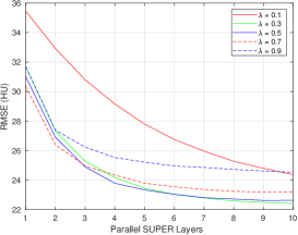
We train the parallel SUPER framework with different choices of the parameter including and to obtain the best choice. Fig. 2 shows the evolution of RMSE over layers for 20 validation slices with different choices. We can see that we obtain the best RMSE when .
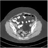
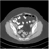
We have conducted experiments on 20 test slices (slice 20, slice 50, slice 100, slice 150 and slice 200 of patient L067, L143, L192, L310) of the Mayo Clinic data. Table I shows the averaged image quality of 20 test images with different methods. From Table I, we observe that Parallel SUPER significantly improves the image quality compared with the standalone methods. It also achieves 1.8 HU better average RMSE compared with Serial SUPER while its SSIM is comparable with Serial SUPER. Fig. 3 shows the reconstructions of L067 (slice 50) and L310 (slice 150) using PWLS-ULTRA, FBPConvNet, serial SUPER (FBPConvNet + PWLS-ULTRA), and parallel SUPER (FBPConvNet + PWLS-ULTRA), along with the references (ground truth). The Parallel SUPER scheme achieved the lowest RMSE and the zoom-in areas show that Parallel SUPER can reconstruct image details better.
| PWLS-EP | PWLS-ULTRA | FBPConvNet | |
|---|---|---|---|
| RMSE | |||
| SSIM | |||
| Serial SUPER | Parallel SUPER | ||
| RMSE | |||
| SSIM |
IV Conclusions
This paper proposes the parallel SUPER framework combining supervised deep learning methods and unsupervised methods for low-dose CT reconstruction. We have experimented on a setting with the supervised model FBPConvNet and the unsupervised model PWLS-ULTRA. This framework demonstrates better reconstruction accuracy and faster convergence compared to individual involved modules as well as the recent serial SUPER framework.
Acknowledgment
The authors thank Dr. Cynthia McCollough, the Mayo Clinic, the American Association of Physicists in Medicine, and the National Institute of Biomedical Imaging and Bioengineering for providing the Mayo Clinic data.
References
- [1] Z. Huang, S. Ye, M. T. McCann, and S. Ravishankar, “Model-based Reconstruction with Learning: From Unsupervised to Supervised and Beyond,” arXiv e-prints, p. arXiv:2103.14528, Mar. 2021.
- [2] L. A. Feldkamp, L. C. Davis, and J. W. Kress, “Practical cone-beam algorithm,” Journal of the Optical Society of America A, vol. 1, no. 6, pp. 612–619, 1984.
- [3] Q. Xu, H. Yu, X. Mou, L. Zhang, J. Hsieh, and G. Wang, “Low-dose X-ray CT reconstruction via dictionary learning,” IEEE Trans. Med. Imag., vol. 31, no. 9, pp. 1682–97, 2012.
- [4] X. Zheng, Z. Lu, S. Ravishankar, Y. Long, and J. A. Fessler, “Low dose ct image reconstruction with learned sparsifying transform,” 2016 IEEE 12th Image, Video, and Multidimensional Signal Processing Workshop (IVMSP), 2017.
- [5] X. Zheng, S. Ravishankar, Y. Long, and J. A. Fessler, “PWLS-ULTRA: An efficient clustering and learning-based approach for low-dose 3D CT image reconstruction,” IEEE Trans. Med. Imag., vol. 37, no. 6, pp. 1498–510, Jun. 2018.
- [6] S. Ravishankar, J. C. Ye, and J. A. Fessler, “Image reconstruction: From sparsity to data-adaptive methods and machine learning,” Proceedings of the IEEE, vol. 108, no. 1, pp. 86–109, 2020.
- [7] K. H. Jin, M. T. Mccann, E. Froustey, and M. Unser, “Deep convolutional neural network for inverse problems in imaging,” IEEE Transactions on Image Processing, vol. PP, no. 99, pp. 4509–4522, 2016.
- [8] E. Kang, W. Chang, J. Yoo, and J. C. Ye, “Deep Convolutional Framelet Denosing for Low-Dose CT via Wavelet Residual Network,” IEEE Trans. Med. Imaging, vol. 37, no. 6, pp. 1358–1369, 2018.
- [9] S. Ye, Z. Li, M. T. Mccann, Y. Long, and S. Ravishankar, “Unified supervised-unsupervised (super) learning for x-ray ct image reconstruction,” IEEE Transactions on Medical Imaging, vol. 40, no. 11, pp. 2986–3001, 2021.
- [10] C. Mccollough, “Tu‐fg‐207a‐04: Overview of the low dose ct grand challenge,” Medical Physics, vol. 43, no. 2, pp. 3759–60, 2016.
- [11] S. Ye, S. Ravishankar, Y. Long, and J. A. Fessler, “Spultra: Low-dose ct image reconstruction with joint statistical and learned image models,” IEEE Transactions on Medical Imaging, vol. 39, no. 3, pp. 729–741, 2020.
- [12] W. Zhou, A. C. Bovik, H. R. Sheikh, and E. P. Simoncelli, “Image quality assessment: from error visibility to structural similarity,” IEEE Trans Image Process, vol. 13, no. 4, 2004.