On Trace of PGD-Like Adversarial Attacks
Abstract
Adversarial attacks pose safety and security concerns to deep learning applications, but their characteristics are under-explored. Yet largely imperceptible, a strong trace could have been left by PGD-like attacks in an adversarial example. Recall that PGD-like attacks trigger the “local linearity” of a network, which implies different extents of linearity for benign or adversarial examples. Inspired by this, we construct an Adversarial Response Characteristics (ARC) feature to reflect the model’s gradient consistency around the input to indicate the extent of linearity. Under certain conditions, it qualitatively shows a gradually varying pattern from benign example to adversarial example, as the latter leads to Sequel Attack Effect (SAE). To quantitatively evaluate the effectiveness of ARC, we conduct experiments on CIFAR-10 and ImageNet for attack detection and attack type recognition in a challenging setting. The results suggest that SAE is an effective and unique trace of PGD-like attacks reflected through the ARC feature. The ARC feature is intuitive, light-weighted, non-intrusive, and data-undemanding.
1 Introduction
Recent studies reveal the vulnerabilities of deep neural networks by adversarial attacks (Kurakin et al., 2016; Madry et al., 2018), where undesired outputs (e.g., misclassification) are triggered by an imperceptible perturbation superimposed on the model input. The attacks pose safety and security concerns for respective applications. The PGD-like attacks, including BIM (Kurakin et al., 2016), PGD (Madry et al., 2018), MIM (Dong et al., 2018), and APGD (Croce & Hein, 2020a), are strong and widely used in the literature, but their characteristics are under-explored.
Yet, we speculate that a strong attack leaves a strong trace in its result, as in the feature maps (Xie et al., 2019a). In this paper, we consider an extremely limited setting – to identify the trace of PGD-like attacks, given an already trained deep neural network and merely a tiny set (e.g., ) of training data, without any change in architecture or weights, nor any auxiliary deep networks. A method effective in such a setting would be less dependent on external models or data, and tends to reveal deeper characteristics of adversarial examples. Expectedly, it is feasible in more scenarios, even when full access to data is impossible, such as Federated Learning (McMahan et al., 2017) and third-party forensics. Meanwhile, it helps us to understand adversarial examples better.
Recall that FGSM (Goodfellow et al., 2015), the foundation of PGD-like attacks, attributes the network vulnerability to “local linearity” being easily triggered by adversarial perturbations. Thus, we conjecture that a network behaves in a greater extent of linearity to adversarial examples than benign (i.e., unperturbed) ones. With the first-order Taylor expansion of a network, “local linearity” implies high gradient proximity in the respective local area. Thus, we can select a series of data points with stable patterns near the input as exploitation vectors using the BIM (Kurakin et al., 2016) attack, and then compute the model’s Jacobian matrices with respect to them. Next, the Adversarial Response Characteristics (ARC) matrix is constructed from these Jacobian matrices reflecting the gradient direction consistency across all exploitation vectors. Unlike benign examples, results of PGD-like attacks trigger Sequel Attack Effect (SAE), leaving higher values in the ARC matrix, reflecting higher gradient consistency around the input. Visualization results suggest SAE is a gradually varying pattern with perturbation magnitude increasing, indicating its effectiveness.

The ARC matrix can be simplified into a -D ARC vector by fitting a Laplacian function due to their resemblance. This simplifies the interpretation of subsequent procedures. The ARC vector can be used for informed attack detection (the perturbation magnitude is known) with an SVM-based binary classifier, or uninformed attack detection (the perturbation magnitude is unknown) with an SVM-based ordinal regression model. The ARC vector can also be used for attack type recognition in similar settings with the same set of SVMs. The SAE reflected through ARC is the unique trace of PGD-like attacks. Due to the uniqueness of SAE to PGD-like attacks, we can also infer attack details, including the loss function and the ground-truth label once the attack is detected.
We evaluate our method on CIFAR-10 (Krizhevsky et al., 2009) with ResNet-18 (He et al., 2015), and ImageNet (Deng et al., 2009) with ResNet-152 (He et al., 2015) / SwinT-B-IN1K (Liu et al., 2021). Qualitative visualizations and quantitative experimental results for attack detection and attack type recognition manifest the effectiveness of our method in identifying SAE. SAE is the unique trace of PGD-like attacks, which also possess considerable generalization capability among PGD-like attacks even if training data only involves a few benign and adversarial examples.
Contributions. We present the ARC features to identify the unique trace, i.e., SAE of PGD-like attacks from adversarially perturbed inputs. It can be used for various applications, such as attack detection and attack type recognition, where inferring attack details is possible. Through the lens of the ARC feature (reflecting the network’s gradient behavior), we also obtain insights on why networks are vulnerable and why adversarial training works well as a defense. Although our method is specific to PGD-like attacks due to strong assumptions, it is (1) intuitive (human-interpretable due to simplicity and not creating a deep model); (2) light-weighted (requires no auxiliary deep model); (3) non-intrusive (requires no change to the network architecture or weights); (4) data-undemanding (can generalize with only a few samples).
2 Adversarial Response Characteristics
A network maps the input into a pre-softmax output , where the maximum element after softmax corresponds to the class prediction , which should match with the ground truth . Then, a typical adversarial attack (Kurakin et al., 2016; Madry et al., 2018) aims to find an imperceptible adversarial perturbation that induces misclassification, i.e., where , , and is the -th element of vector function .


According to (Goodfellow et al., 2015), a neural network is vulnerable as the “locally linear” property is triggered by attack. Thus, we assume that the network behaves relatively non-linear against benign examples, while relatively linear against adversarial examples. Then, can be approximated by the first-order Taylor expansion around an either benign or adversarial sample :
| (1) |
where is a small vector exploiting the local area around the point , and the gradient vector is the -th row of the Jacobian of size . We name the twice-perturbed as “exploitation vector”. This equation means in order to reflect linear behavior, the first-order gradient is expected to remain in high consistency (or similarity) in the local area regardless of . In contrast, when the input is not adversarial (), neither Taylor approximation nor the gradient consistency is expected to hold. Next, the gradient consistency will be quantized to verify our conjecture, and reveal the difference between benign and adversarial inputs.
Adversarial Response Characteristics (ARC). Using random noise as does not lead to a stable pattern of change in a series of exploitation vectors . Instead, we use Basic Iterative Method (BIM) (Kurakin et al., 2016) to make more linear starting from , which means to “continue” the attack if is already adversarial, or “restart” otherwise. However, the ground-truth label for an arbitrary is unknown. Since PGD-like attacks tend to make the ground-truth least-likely based on our observation, we treat the least-likely prediction as the label. Then, the BIM iteratively maximizes the cross entropy loss via projected gradient ascent as
| (2) |
where clips the perturbation to the bound centered at , and . If the input is benign, then the network behavior is expected to change from “very non-linear“ to “somewhat-linear” during the process; if the input is already adversarially perturbed, then the process will “continue” the attack, making the model even more “linear” – we call this Sequel Attack Effect (SAE).
To quantize the extent of “linearity”, we measure the model’s gradient consistency across exploitation vectors with cosine similarity. For each , we construct a matrix of shape :
| (3) |
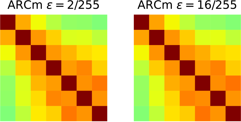
As the model becomes more “linear” to the input (higher gradient consistency), the off-diagonal values in are expected to gradually increase from the top-left to the bottom-right corner. Note that the attack may not necessarily make all behave linear, so we select the most representative cosine matrix with the highest mean as the ARC matrix: , where .
Due to the resemblance of the ARC matrix to the Laplacian function with the matrix diagonal being the center, we simplify it into a two-dimensional ARC vector by fitting with Levenberg-Marquardt algorithm (Virtanen et al., 2020), where are matrix row and column indexes, while and are function parameters. For brevity, we abbreviate the ARC matrix as “ARCm”, and the ARC vector as “ARCv”. The overall process is summarized in Fig. 1.
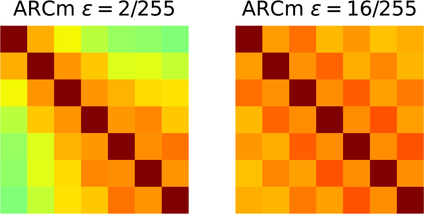
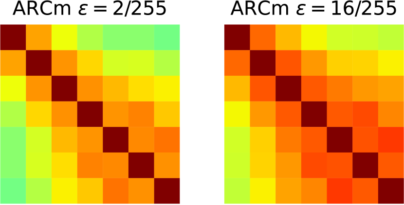
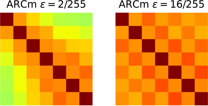
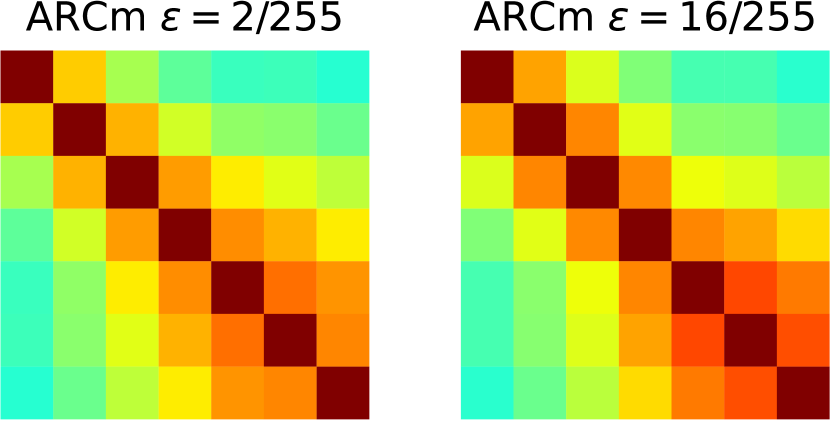
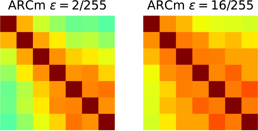
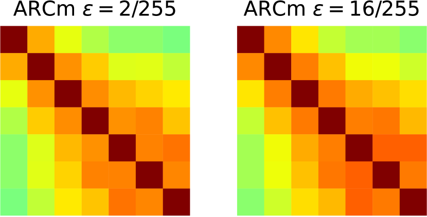
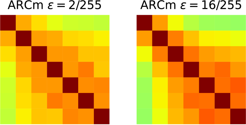
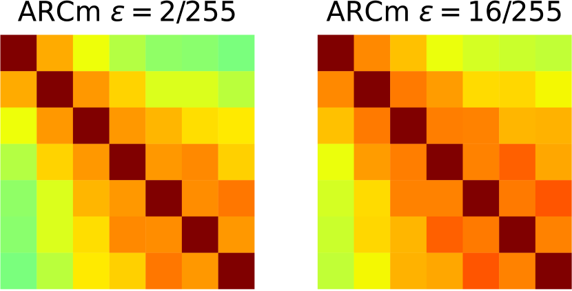
Visualizing Sequel Attack Effect (SAE). We compute ARCm based on some benign examples using , as shown in Fig. 1. The trend of being gradually “linear” (higher cosine similarity) along the diagonal is found across architectures. Thus, SAE is similar to “continuing” an attack from halfway on the diagonal in such a large ARCm. As illustrated in Fig. 2, already adversarially perturbed input (using BIM) leads to larger cosine similarity at the very first exploitation vectors as perturbation magnitude increases from to . Meanwhile, the cluster separation for ARCv is more and more clear. Thus, a clear and gradually changing pattern can be seen in ARCm and ARCv. This pattern is even valid and clear for the state-of-the-art ImageNet models. In brief, SAE is reflected by higher gradient consistency in ARCm, or greater and smaller in ARCv. Similar results for other PGD-like attacks in Fig. 3 indicate the possibility of generalization among them with only training samples from the BIM attack. We adopt SVM afterward to retain interpretability and simplicity.


Uniqueness of SAE to PGD-Like Attack. Whether SAE can be consistently triggered depends on the following conditions simultaneously being true: (I) whether the input is adversarially perturbed by an iterative projected gradient update method for many steps; (II) whether the attack leverages the first-order gradient of the model; (III) whether the boundary types are the same for the two stages, i.e., attack and exploitation vectors; (IV) whether the loss functions for the two stages are the same; (V) whether the labels used (if any) for the two stages are relevant. Namely, only when the attack and exploitation vectors “match”, can SAE be uniquely triggered as the exploitation vectors “continue” an attack, or they will “restart” an attack. Thus, in Fig. 1, Fig. 2 and Fig. 3, all the conditions are true as they involve PGD-like attacks. Due to the strong assumptions, the SAE being insensitive to non-PGD-like attacks (e.g., Carlini & Wagner (2017b)) is a limitation. However, the unique SAE meanwhile shows a possibility of inferring the attack details leveraging the above conditions. SAE is the trace of PGD-like attacks. Ablations for these five conditions are presented in Sec. 5.
Adaptive Attack.
Adaptive attacks can be designed against defenses (Tramer et al., 2020),
detection (Carlini & Wagner, 2017a).
To avoid SAE in ARCm, an adaptive attack must reach a point
where the corresponding ARCm has a mean value as small as that for
benign examples.
Intuitively, an adaptive attack has to simultaneously solve
(Frobenius norm) alongside its original attack goal.
It however requires the gradient of Jacobians, namely at least Hessian
matrices, i.e., of size
to perform gradient descent.
This is computationally prohibitive as in the typical ImageNet setting
(i.e., ), a Hessian in float32 precision
needs GiB memory.
At this point, the cost of adaptive attack that hides SAE is much higher than
computing ARC.
Instead, a viable way to avoid SAE is to use non-PGD-like attacks
that break the SAE uniqueness conditions.
This paper focuses on characterizing the unique trace of existing
PGD-like attacks, instead of a general detection or defense method.
3 Applications of ARC Feature
In order to quantitatively support the effectiveness of ARC/SAE, we adopt it for two potential tasks, namely attack detection and attack type recognition. Attack detection aims to identify the attempt to adversarially perturb an image even if it fails to change the prediction (but leaves a trace).111 In practice, it is undesirable to wait and react until the attack has succeeded. Attack type recognition aims to identify whether an adversarial example is created by PGD-like attacks. Our method relies on the uniqueness of SAE to PGD-like attacks for the two tasks.
Informed Attack Detection determines whether an arbitrary input is adversarially perturbed, while the perturbation magnitude is known. It can be viewed as a binary classification problem, where the input is ARCv of , and the output indicates “adversarially perturbed”, while indicates “unperturbed”. Thus, for a given where , a corresponding SVM (Pedregosa et al., 2011) classifier can be trained using some benign () samples and their adversarial counterparts (). Even if the training data only involves the BIM attack, we expect generalization for other PGD-like attacks from visualization results despite domain shift.
Uninformed Attack Detection determines whether an arbitrary input is adversarially perturbed, while the perturbation magnitude is unknown. It can be viewed as an ordinal regression (Niu et al., 2016) problem, where the input is ARCv, and the output is the estimation of , namely . The corresponding estimate of is , where is the indicator function. Specifically, this is implemented as a series of binary classifiers (SVM), where the -th () classifier predicts whether the level of perturbation is greater or equal to , i.e., whether . Note, based on our visualization, the ARCv cluster of adversarial examples is moving away from that of benign examples as (or ) increases. This means the ARCv of an adversarial example with will also cross the decision boundary of the -th SVM . Namely the SVM can also tell whether , and thus can be reused. Finally, the ordinal regression model can be expressed as the sum of prediction over the SVMs: . A perturbation is detected as long as . Estimating (or ) for is similar to matching its ARCm position inside a much larger ARCm calculated starting from a benign example. But, the estimate does not have to be precise, because the detection is already successful once any of the SVMs correctly raises an alert.
Although a detector in practice knows completely nothing about a potential attack including the attack type, evaluation of uninformed attack detection with known attack type is enough. Regarding the performance for uninformed attack detection given a specific attack type as a conditional performance, the expected performance in the wild can be calculated as the sum of conditional performance weighted by the prior probabilities that the corresponding attack happens.
Inferring Attack Details. Due to the SAE uniqueness in Sec. 2, once the attack is detected, we can also predict that the attack: (I) performs projected gradient update iteratively; (II) uses the first-order gradient of ; (III) uses the same type of bound as exploitation vectors ( by default); (IV) uses the same loss as exploitation vectors ( by default); (V) uses a ground-truth label which is relevant to the least-likely class used for exploitation vectors (in many cases is exactly the ground-truth). In other words, model prediction can be corrected into the least-likely class upon detection. Namely, the disadvantage of ARC being insensitive to non-PGD-like attacks is meanwhile advantage of being able to infer attack details of PGD-like attacks.
Attack Type Recognition determines whether an adversarial input is created by PGD-like attacks in the uninformed setting for forensics purposes. The corresponding binary classifier can be built upon the previously discussed detectors, because SAE only responds to PGD-like attacks.
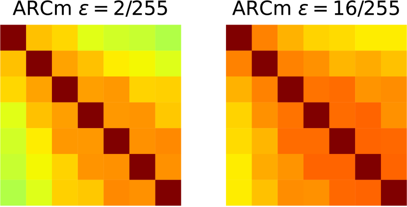
BIM[DLR]; ARC[DLR]
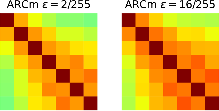
SPSA[✗]; ARC[]
4 Experiments
In this section, we quantitatively verify the effectiveness of the ARC features in two applications, and the effectiveness of the post-processing step under an extremely limited setting. Unlike related works, the MNIST evaluation is omitted, as the corresponding conclusions may not hold (Carlini & Wagner, 2017a) on CIFAR-10, let alone ImageNet. We evaluate ResNet-18 (He et al., 2015) on CIFAR-10 (Krizhevsky et al., 2009); ResNet-152 (He et al., 2015) and SwinT-B-IN1K (Liu et al., 2021) on ImageNet (Deng et al., 2009) with their official pre-trained weights (advantage of being non-intrusive). Our code is implemented based on PyTorch (Paszke et al., 2019).
ARC Feature Parameter. For the BIM attack for exploitation vectors, we set step number , and step size under the bound with . Note, the mean value of ARCm will tend to with a larger , making ARCv less separatable. We choose to clearly visualize the value changes within ARCm, but this does not necessarily lead to the best performance.
Training. We train SVMs with RBF kernel. We randomly select training samples from CIFAR-10, and perturb them using only BIM with magnitude , respectively. Then each of the four is trained with ARCv of the benign () samples and perturbed () samples. Likewise, for ImageNet we randomly select training samples and train SVM in a similar setting separately for ResNet-152 and SwinT-B-IN1K. The weight for benign examples can be adjusted for training to control the False Positive Rate (FPR).
Testing. For CIFAR-10, all testing data and their perturbed versions with different are used to test our SVM. For ImageNet, we randomly choose testing samples due to costly Jacobian computation. A wide range of adversarial attacks are involved, including (1) PGD-like attacks: BIM (Kurakin et al., 2016), PGD (Madry et al., 2018), MIM (Dong et al., 2018), APGD (Croce & Hein, 2020a), AutoAttack (AA) (Croce & Hein, 2020a); (2) Non-PGD-like attacks: (2.1) other white-box attacks: FGSM (Goodfellow et al., 2015), C&W (Carlini & Wagner, 2017b) (we use in case), FAB (Croce & Hein, 2020b), FMN (Pintor et al., 2021); (2.2) transferability attacks: DI-FGSM (Xie et al., 2019b), TI-FGSM (Dong et al., 2019) (using ResNet-50 as proxy); (2.3) score-based black-box methods: NES (Ilyas et al., 2018), SPSA (Uesato et al., 2018), Square (Andriushchenko et al., 2020). AutoAttack is regarded as PGD-like because APGD is its most significant component for success rate. Details can be found in the supplementary code.
Metrics. The SVMs are evaluated with Detection Rate (DR, a.k.a., True Positive Rate) and False Positive Rate (FPR). For inferring the ground-truth label, we report the original accuracy for perturbed examples (denoted as “Acc”) and that after correction (denoted as “Acc*”). Mean Average Error (MAE) is also reported for ordinal regression. Accuracy is reported for attack type recognition.
4.1 Application of ARC: Attack Detection
| Dataset Model | Attack | |||||||||||||||||||||
|---|---|---|---|---|---|---|---|---|---|---|---|---|---|---|---|---|---|---|---|---|---|---|
| DR | FPR | Acc | Acc* | DR | FPR | Acc | Acc* | DR | FPR | Acc | Acc* | DR | FPR | Acc | Acc* | MAE | DR | FPR | Acc | Acc* | ||
| CIFAR-10 ResNet-18 | BIM | 0.0 | 0.0 | 33.5 | 33.5 | 0.0 | 0.0 | 6.4 | 6.4 | 32.3 | 1.5 | 0.4 | 17.8 | 79.2 | 1.1 | 0.0 | 62.4 | 1.55 | 30.9 | 1.5 | 10.1 | 30.7 |
| PGD | 0.0 | 0.0 | 33.7 | 33.7 | 0.0 | 0.0 | 6.4 | 6.4 | 33.0 | 1.5 | 0.4 | 18.6 | 81.2 | 1.1 | 0.0 | 64.8 | 1.54 | 31.5 | 1.5 | 10.1 | 31.5 | |
| MIM | 0.0 | 0.0 | 30.4 | 30.4 | 0.0 | 0.0 | 6.5 | 6.5 | 37.5 | 1.5 | 0.4 | 22.3 | 84.5 | 1.1 | 0.0 | 67.4 | 1.50 | 33.6 | 1.5 | 9.3 | 32.4 | |
| APGD | 0.0 | 0.0 | 29.3 | 29.3 | 0.0 | 0.0 | 5.1 | 5.1 | 36.9 | 1.5 | 0.2 | 20.7 | 78.8 | 1.1 | 0.0 | 55.8 | 1.53 | 31.5 | 1.5 | 8.7 | 28.0 | |
| AA | 0.0 | 0.0 | 27.4 | 27.4 | 0.0 | 0.0 | 2.1 | 2.1 | 37.3 | 1.5 | 0.0 | 20.6 | 78.4 | 1.1 | 0.0 | 55.6 | 1.53 | 31.6 | 1.5 | 7.4 | 26.8 | |
| ? | 0.0 | 0.0 | 30.9 | 30.9 | 0.0 | 0.0 | 5.3 | 5.3 | 35.4 | 1.5 | 0.3 | 20.0 | 80.4 | 1.1 | 0.0 | 61.2 | 1.53 | 31.8 | 1.5 | 9.1 | 29.9 | |
| ImageNet ResNet-152 | BIM | 0.0 | 0.0 | 0.0 | 0.0 | 4.7 | 1.4 | 0.0 | 0.0 | 20.5 | 1.4 | 0.0 | 0.0 | 91.6 | 1.4 | 0.0 | 0.4 | 1.36 | 30.6 | 1.6 | 0.0 | 0.1 |
| PGD | 0.0 | 0.0 | 0.0 | 0.0 | 4.7 | 1.4 | 0.0 | 0.0 | 18.8 | 1.4 | 0.0 | 0.0 | 85.9 | 1.4 | 0.0 | 0.0 | 1.44 | 28.9 | 1.6 | 0.0 | 0.0 | |
| MIM | 0.0 | 0.0 | 0.0 | 0.0 | 2.3 | 1.4 | 0.0 | 0.0 | 4.7 | 1.4 | 0.0 | 0.0 | 81.2 | 1.4 | 0.0 | 0.0 | 1.52 | 23.8 | 1.6 | 0.0 | 0.2 | |
| APGD | 0.0 | 0.0 | 0.0 | 0.0 | 2.0 | 1.4 | 0.0 | 0.0 | 11.3 | 1.4 | 0.0 | 0.0 | 61.7 | 1.4 | 0.0 | 0.4 | 1.59 | 19.7 | 1.6 | 0.0 | 0.1 | |
| AA | 0.0 | 0.0 | 0.0 | 0.0 | 2.5 | 1.4 | 0.0 | 0.0 | 10.7 | 1.4 | 0.0 | 0.0 | 61.5 | 1.4 | 0.0 | 0.0 | 1.59 | 19.9 | 1.6 | 0.0 | 0.0 | |
| ? | 0.0 | 0.0 | 0.0 | 0.0 | 3.2 | 1.4 | 0.0 | 0.0 | 13.2 | 1.4 | 0.0 | 0.0 | 76.3 | 1.4 | 0.0 | 0.2 | 1.50 | 24.6 | 1.6 | 0.0 | 0.1 | |
| ImageNet SwinT-B-IN1K | BIM | 4.1 | 1.6 | 6.1 | 6.2 | 13.7 | 2.0 | 0.0 | 8.4 | 77.3 | 2.0 | 0.0 | 74.0 | 97.9 | 0.2 | 0.0 | 97.9 | 0.96 | 49.1 | 2.0 | 1.5 | 47.3 |
| PGD | 3.9 | 1.6 | 2.3 | 3.1 | 16.4 | 2.0 | 0.0 | 10.9 | 72.7 | 2.0 | 0.0 | 68.8 | 98.4 | 0.2 | 0.0 | 98.4 | 1.01 | 48.6 | 2.0 | 0.6 | 45.9 | |
| MIM | 1.6 | 1.6 | 0.0 | 1.6 | 10.2 | 2.0 | 0.0 | 10.2 | 63.3 | 2.0 | 0.0 | 63.3 | 93.8 | 0.2 | 0.0 | 93.8 | 1.09 | 43.8 | 2.0 | 0.0 | 43.8 | |
| APGD | 1.4 | 1.6 | 0.0 | 1.0 | 5.3 | 2.0 | 0.0 | 4.5 | 32.6 | 2.0 | 0.0 | 25.2 | 65.0 | 0.2 | 0.0 | 51.0 | 1.37 | 29.4 | 2.0 | 0.0 | 23.2 | |
| AA | 1.8 | 1.6 | 0.0 | 1.0 | 5.7 | 2.0 | 0.0 | 4.3 | 31.6 | 2.0 | 0.0 | 25.0 | 68.4 | 0.2 | 0.0 | 54.1 | 1.37 | 29.5 | 2.0 | 0.0 | 23.2 | |
| ? | 2.6 | 1.6 | 1.7 | 2.6 | 10.2 | 2.0 | 0.0 | 7.7 | 55.5 | 2.0 | 0.0 | 51.2 | 84.7 | 0.2 | 0.0 | 79.0 | 1.16 | 40.1 | 2.0 | 0.4 | 36.7 | |
For each network, the corresponding SVMs are trained and evaluated as shown in Tab. 1. Columns with a concrete value are informed attack detection, while the ““ column is uninformed attack detection. As can be expected from visualization results, the ARCv clusters are gradually becoming separatable with increasing, hence the increase of DR. Notably, the large perturbations (i.e., ) are hard to defend (Qin et al., 2019), but can be consistently detected across architectures. The ARC feature is especially effective for Swin-Transformer, because this model transitions faster from being non-linear to being linear than other architectures. Such characteristics are beneficial for SAE.
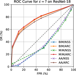
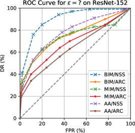
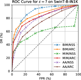
Upon detection of an attack, our method can correct the prediction into the least-likely class as a post-processing step. Its success rate depends on whether the attack is efficient to make the ground-truth class least-likely, and whether the network is easy for the attack to make a class least-likely. From Tab. 1, both ResNet-18 and SwinTransformer have such a property and lead to high classification accuracy after correction. For ResNet-152, the least-likely label is merely relevant (not identical) to the ground truth due to network property during attack, hence leading to effective detection but not correction (this will be explained in the next subsection). In contrast, the correction method performs best on Swin-Transformer, as it can restore classification accuracy from to even if both the concrete type of PGD-like attack and are unknown (“Attack=?” row and “” column in Tab. 1), assuming flat prior. By adjusting the weights assigned to benign examples, the decision boundary of SVMs can be moved and hence influence the FPR, as shown in Fig. 5.
4.2 Sequel Attack Effect as Unique Trace of PGD-like Attacks
| # | Attack | ARC | ResNet-18 w/ | ResNet-152 w/ | SwinT-B-IN1K w/ | ||||||||||||||||||
| Name | Loss | Iter. | Loss | Label | MAE | DR | FPR | Acc | Acc* | MAE | DR | FPR | Acc | Acc* | MAE | DR | FPR | Acc | Acc* | ||||
| t1 | BIM | CE | Yes | Yes | CE | 1.55 | 30.9 | 1.5 | 10.1 | 30.7 | 1.36 | 30.6 | 1.6 | 0.0 | 0.1 | 0.96 | 49.1 | 2.0 | 1.5 | 47.3 | |||
| t2 | BIM | 2 | .. | .. | .. | .. | .. | .. | 1.27 | 49.9 | 1.5 | 2.6 | 39.0 | 1.98 | 3.5 | 1.6 | 0.2 | 0.2 | 2.02 | 1.0 | 2.0 | 1.4 | 1.8 |
| t3 | BIM | .. | DLR | .. | .. | .. | .. | .. | 1.98 | 2.1 | 1.5 | 10.5 | 10.6 | 1.63 | 18.9 | 1.6 | 0.0 | 0.6 | 1.44 | 27.5 | 2.0 | 1.8 | 6.6 |
| t4 | FGSM | .. | .. | No | .. | .. | .. | .. | 1.96 | 3.4 | 1.5 | 30.3 | 29.5 | 1.63 | 18.6 | 1.6 | 8.4 | 6.8 | 1.44 | 27.1 | 2.0 | 44.9 | 32.4 |
| t5 | C&W | C&W | .. | .. | .. | .. | .. | 1.99 | 1.2 | 1.5 | 0.0 | 0.0 | 2.02 | 2.3 | 1.6 | 0.0 | 0.0 | 2.03 | 1.6 | 2.0 | 0.0 | 0.0 | |
| t6 | FAB | .. | FAB | .. | .. | .. | .. | .. | 1.99 | 1.0 | 1.5 | 10.6 | 10.5 | 2.00 | 2.5 | 1.6 | 9.2 | 9.2 | 2.03 | 0.8 | 2.0 | 9.4 | 9.4 |
| t7 | FMN | .. | FMN | .. | .. | .. | .. | .. | 1.99 | 1.4 | 1.5 | 8.8 | 8.6 | 2.02 | 2.1 | 1.6 | 0.0 | 0.0 | 2.03 | 0.8 | 2.0 | 0.0 | 0.0 |
| t8 | DI-FGSM | .. | DI-FGSM | .. | No | .. | .. | .. | 1.98 | 2.2 | 1.5 | 42.9 | 42.0 | 1.98 | 3.5 | 1.6 | 27.9 | 27.5 | 1.87 | 8.2 | 2.0 | 67.2 | 62.1 |
| t9 | TI-FGSM | .. | TI-FGSM | .. | No | .. | .. | .. | 1.98 | 1.9 | 1.5 | 59.4 | 58.3 | 2.00 | 2.9 | 1.6 | 40.0 | 39.1 | 2.02 | 1.6 | 2.0 | 72.3 | 70.9 |
| t10 | NES | .. | .. | .. | No | .. | .. | .. | 1.94 | 4.7 | 1.5 | 38.6 | 39.4 | 1.98 | 3.1 | 1.6 | 28.3 | 27.3 | 2.02 | 1.6 | 2.0 | 50.6 | 49.4 |
| t11 | SPSA | .. | .. | .. | No | .. | .. | .. | 1.97 | 3.0 | 1.5 | 39.2 | 39.1 | 2.00 | 3.1 | 1.6 | 29.9 | 28.9 | 2.00 | 2.7 | 2.0 | 52.7 | 50.6 |
| t12 | Square | .. | Square | .. | No | .. | .. | .. | 1.99 | 1.6 | 1.5 | 85.7 | 84.3 | 2.02 | 2.1 | 1.6 | 68.6 | 67.4 | 1.84 | 10.2 | 2.0 | 77.9 | 70.1 |
| t13 | Gaussian | .. | N/A | No | No | .. | .. | .. | 1.99 | 1.7 | 1.5 | 87.0 | 85.6 | 2.00 | 2.7 | 1.6 | 75.2 | 73.2 | 2.00 | 3.1 | 2.0 | 82.4 | 79.7 |
| t14 | Uniform | .. | N/A | No | No | .. | .. | .. | 1.99 | 1.8 | 1.5 | 86.6 | 85.0 | 1.97 | 4.1 | 1.6 | 73.6 | 70.9 | 1.84 | 10.2 | 2.0 | 81.8 | 73.2 |
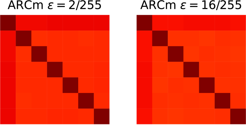
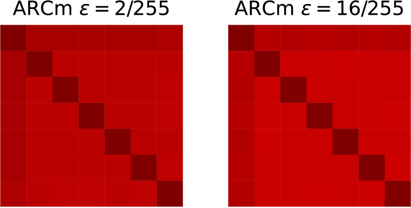
The SAE is unique to PGD-like attacks, as it requires five conditions listed in Sec. 2 to hold for consistent effectiveness. To clarify this, we change the attack settings (quantitatively in Tab. 2), or the exploitation vector for ARCm (qualitatively on CIFAR10 in Fig. 4), and then review these conditions:
-
(I).
Iterative attack (Iter.). The single-step version of PGD, i.e., FGSM (t4, f4) does not effectively exploit the search space within the bound, and hence will not easily trigger linearity and SAE. Only Swin Transformer slightly reacts against FGSM due to its own characteristics of being easy to be turned linear. Thus, SAE requires the attack to be iterative;
-
(II).
Gradient access (). Transferability-based attacks (t8, t9) use proxy model gradients to create adversarial examples, and hence could not trigger SAE. NES (t10, f14) and SPSA (t11, f15) can be seen as PGD using gradients estimated from only network logits, but can still not trigger SAE as it cannot efficiently trigger linearity. Neither does Square attack (t12). Thus, SAE requires that the attacks use the target model gradient;
-
(III).
Same bound. When the attack is BIM in bound (t2, f6), SAE will no longer be triggered for ImageNet models, because the change of influences the perturbation search process. However, SAE is still triggered for CIFAR-10 possibly due to relatively low-dimensional search space. This means CIFAR-10 property does not necessarily generalize to ImageNet. When ARC has been changed accordingly (f7, f8), the feature clusters are still separatable. Thus, SAE requires the same type of bound for consistent effectiveness;
-
(IV).
Same loss. When the loss for BIM is switched from to DLR (Croce & Hein, 2020a) (t3, f11), the SAE is significantly reduced. However, if exploitation vectors are also created using DLR (f12, f13), SAE will be triggered again. Thus, SAE requires a consistent loss;
-
(V).
Relevant label. When the most-likely label is used for exploitation vectors, it leads to the least significant SAE (f9). Besides, even a random label () leads to moderate SAE (f10), while the least-likely label (which is ground-truth label in many cases) leads to distinct SAE (f1). The most significant SAE correspond to . This means that to maximize cross-entropy, the local linearity of a large portion of output functions has been triggered. Thus, SAE requires a relevant label (if any) for exploitation vectors.
When the exploitation vectors are created using random noise (f2, f3), SAE is not triggered. Neither does random noise as an attack trigger SAE (t13, t14, f5). Other non-PGD-like attacks (t5, t6, t7) do not trigger SAE either. A special case is targeted PGD-like attack, where the creation of exploitation vectors needs to use negative cross-entropy loss on the most-likely label to reach a similar level of effectiveness (this paper focuses on the default untargeted attack to avoid complication).
The non-PGD attacks, or PGD variants do not meet all conditions cannot consistently trigger SAE across architectures because they provide a less “matching” starting point for exploitation vectors, and hence make the BIM for exploitation vectors “restart” an attack, where the network behaves non-linear again. Only when all the conditions are satisfied will SAE be consistently triggered across different architectures, especially for ImageNet models. As for label correction, PGD-like attacks can effectively leak the ground-truth labels in the adversarial example, as long as the network allows the attack to easily reduce the corresponding logit value to the lowest.
4.3 Comparison with Previous Attack Detection Methods
| Method | Metric | BIM | PGD | MIM | APGD | AA | ||||||||||||||||||||
| 2/255 | 4/255 | 8/255 | 16/255 | ? | 2/255 | 4/255 | 8/255 | 16/255 | ? | 2/255 | 4/255 | 8/255 | 16/255 | ? | 2/255 | 4/255 | 8/255 | 16/255 | ? | 2/255 | 4/255 | 8/255 | 16/255 | ? | ||
| CIFAR10 ResNet-18 | ||||||||||||||||||||||||||
| NSS (Kherchouche et al., 2020) | DR | 0.0 | 0.0 | 0.0 | 0.1 | 0.5 | 0.0 | 0.0 | 0.0 | 0.1 | 0.5 | 0.0 | 0.0 | 0.0 | 0.1 | 4.7 | 0.0 | 0.0 | 0.3 | 0.2 | 0.8 | 0.0 | 0.0 | 0.3 | 0.2 | 0.8 |
| FPR | 0.0 | 0.0 | 1.8 | 1.5 | 2.5 | 0.0 | 0.0 | 1.8 | 1.5 | 2.5 | 0.0 | 0.0 | 1.8 | 1.5 | 2.5 | 0.0 | 0.0 | 1.8 | 1.5 | 2.5 | 0.0 | 0.0 | 1.8 | 1.5 | 2.5 | |
| ARC | DR | 0.0 | 0.0 | 32.3 | 79.2 | 30.9 | 0.0 | 0.0 | 33.0 | 81.2 | 31.5 | 0.0 | 0.0 | 37.5 | 84.5 | 33.6 | 0.0 | 0.0 | 36.9 | 78.8 | 31.5 | 0.0 | 0.0 | 37.3 | 78.4 | 31.6 |
| FPR | 0.0 | 0.0 | 1.5 | 1.1 | 1.5 | 0.0 | 0.0 | 1.5 | 1.1 | 1.5 | 0.0 | 0.0 | 1.5 | 1.1 | 1.5 | 0.0 | 0.0 | 1.5 | 1.1 | 1.5 | 0.0 | 0.0 | 1.5 | 1.1 | 1.5 | |
| ImageNet ResNet-152 | ||||||||||||||||||||||||||
| NSS (Kherchouche et al., 2020) | DR | 2.9 | 19.1 | 39.6 | 47.2 | 41.6 | 2.9 | 19.9 | 39.6 | 46.5 | 41.1 | 4.2 | 31.2 | 41.4 | 9.1 | 32.9 | 1.1 | 12.6 | 28.3 | 35.7 | 29.1 | 1.0 | 11.9 | 29.8 | 33.3 | 28.7 |
| FPR | 0.4 | 1.4 | 1.2 | 1.4 | 2.0 | 0.4 | 1.4 | 1.2 | 1.4 | 2.0 | 0.4 | 1.4 | 1.2 | 1.4 | 2.0 | 0.6 | 1.4 | 1.2 | 1.4 | 2.0 | 0.4 | 1.4 | 1.2 | 1.4 | 2.0 | |
| ARC | DR | 0.0 | 4.7 | 20.5 | 91.6 | 30.6 | 0.0 | 4.7 | 18.8 | 85.9 | 28.9 | 0.0 | 2.3 | 4.7 | 81.2 | 23.8 | 0.0 | 2.0 | 11.3 | 61.7 | 19.7 | 0.0 | 2.5 | 10.7 | 61.5 | 19.9 |
| FPR | 0.0 | 1.4 | 1.4 | 1.4 | 1.6 | 0.0 | 1.4 | 1.4 | 1.4 | 1.6 | 0.0 | 1.4 | 1.4 | 1.4 | 1.6 | 0.0 | 1.4 | 1.4 | 1.4 | 1.6 | 0.0 | 1.4 | 1.4 | 1.4 | 1.6 | |
| ImageNet SwinT-B-IN1K | ||||||||||||||||||||||||||
| NSS (Kherchouche et al., 2020) | DR | 4.5 | 16.2 | 42.4 | 47.5 | 44.2 | 4.9 | 15.8 | 41.8 | 47.1 | 44.1 | 12.3 | 28.7 | 29.3 | 4.5 | 28.9 | 1.6 | 11.0 | 31.3 | 35.5 | 31.1 | 1.4 | 10.4 | 31.8 | 35.1 | 30.8 |
| FPR | 0.6 | 1.0 | 1.2 | 1.6 | 2.3 | 0.6 | 1.0 | 1.2 | 1.6 | 2.3 | 0.6 | 1.0 | 1.2 | 1.5 | 2.3 | 0.6 | 1.0 | 1.2 | 1.6 | 2.3 | 0.6 | 1.0 | 1.2 | 1.6 | 2.3 | |
| ARC | DR | 4.1 | 13.7 | 77.3 | 97.9 | 49.1 | 3.9 | 16.4 | 72.7 | 98.4 | 48.6 | 1.6 | 10.2 | 63.3 | 93.8 | 43.8 | 1.4 | 5.3 | 32.6 | 65.0 | 29.4 | 1.8 | 5.7 | 31.6 | 68.4 | 29.5 |
| FPR | 1.6 | 2.0 | 2.0 | 0.2 | 2.0 | 1.6 | 2.0 | 2.0 | 0.2 | 2.0 | 1.6 | 2.0 | 2.0 | 0.2 | 2.0 | 1.6 | 2.0 | 2.0 | 0.2 | 2.0 | 1.6 | 2.0 | 2.0 | 0.2 | 2.0 | |
As discussed in Sec. 6, due to our extremely limited problem setting – (1) no auxiliary deep model; (2) non-intrusive; (3) data-undemanding, the most relevant methods that do not lack ImageNet evaluation are Kherchouche et al. (2020); Roth et al. (2019); Li & Li (2017); Lu et al. (2017); Ma & Liu (2019). But Roth et al. (2019); Li & Li (2017); Lu et al. (2017); Ma & Liu (2019) still require a considerable amount of data to build accurate (relatively) high-dimensional statistics. The remaining NSS (Kherchouche et al., 2020) method craft Natural Scene Statistics features, which are fed into SVM for binary classification. We also adopt the trained SVMs in our ordinal regression framework, with a reduced training set size to ( benign + BIM adversarial) for each SVM for a fair comparison. All SVMs are tuned to control FPR. The results and ROC curves for “” task can be found Tab. 3 and Fig. 5. It is noted that (1) SVM with the -D NSS feature may fail to generalize due to insufficient sampling (hence the below-diagonal ROC); (2) NSS performs better for small , but performance saturates with larger , because NSS does not incorporate any cue from network gradient behavior; (3) small is difficult for ARC, but its performance soars with larger towards , which is consistent and expected from our visualization; (4) SVM with ARCv can generalize against all PGD-like attacks, while NSS failed for MIM; (5) SVM with NSS may generalize against some non-PGD-like attacks (Kherchouche et al., 2020), but not ARC due to SAE uniqueness; (6) SVM with the -D NSS feature (“Method 2” in Kherchouche et al. (2020)) fails to generalize. Thus, ARC achieves competitive performance consistently across different settings despite the extreme limits, because it is low-dimensional, and incorporates effective cues from gradients.
4.4 Application of ARC: Attack Type Recognition
By gathering the sets ( sets from Tab. 1 and sets from Tab. 2 t4-t12) of adversarial examples involved in Tab. 1 and Tab. 2, we can construct a test dataset for attack type recognition. Since each set has an equal number of samples, the binary classification accuracy can be calculated as the average of the DR for PGD-like attacks and for non-PGD-like attacks in the “” setting. The results are , , for ResNet-18, ResNet-152, SwinT-B-IN1K, respectively.
5 Discussions and Justifications


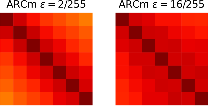
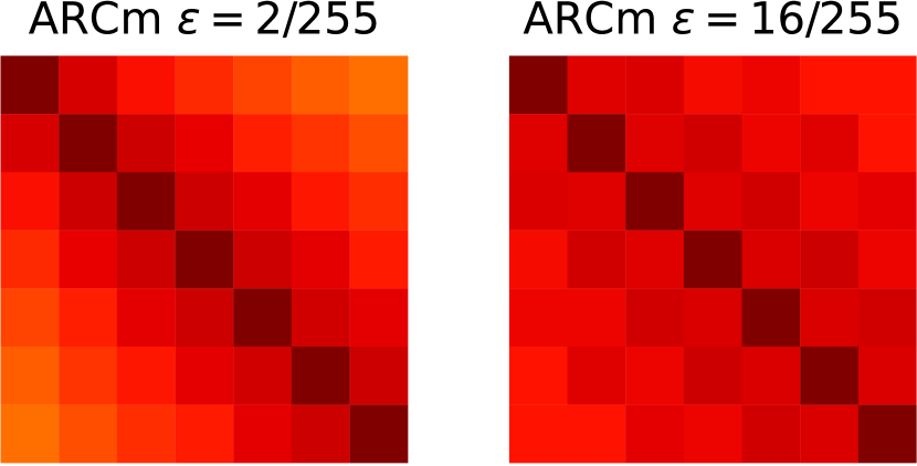
Combination with Adversarial Training. From our experiment and recent works (Madry et al., 2018; Engstrom et al., 2019; Qin et al., 2019), its noted that (1) small perturbations are hard to detect, but easy to defend; while (2) large perturbations are hard to defend, but easy to detect. However, combining defense and our detection is not effective on ImageNet. As shown in Fig. 6, we compute ARCm based on regular ResNet-50 (from PyTorch (Paszke et al., 2019)) and adversarially trained ResNet-50 on ImageNet (from (Engstrom et al., 2019)). Unlike the regular ResNet-50, adversarially trained one has a much higher mean value in ARCm, resulting in almost non-separatable ARCv. This means adversarial training makes the model very linear around the data (Roth et al., 2020). Namely, the network is trained to generalize while being already very linear to the input, and thus it will be hard to make the model behave even more linear to manipulate the output by the attack.
Limitations. This paper focuses on characterizing a specific type of adversarial example instead of a general detection or defense method. The following are the major limitations of the ARC feature in potential applications: (1) The SAE is unique but specific to PGD-like attacks; (2) Jacobian computation is very slow for ImageNet models because it requires iterations of backward pass. We are unable to evaluate our method on all ImageNet data with Nvidia Titan Xp GPUs.
Further Discussions and justifications involving ordinal regression, training set size, and iterations of attacks can be found in the appendix. Experiment details can be found in the supplementary code.
6 Related Works
Adversarial Attack & Defense. Neural networks are found vulnerable (Szegedy et al., 2013; Goodfellow et al., 2015). Based on this, attacks with different threat models are designed, including white-box attacks, transferability attacks, and black-box attacks (Dong et al., 2020). Ilyas et al. (2019) attribute the existence of adversarial examples to non-robust features. To counter the attacks, adversarial training (Madry et al., 2018; Qin et al., 2019; Wu et al., 2020) is the most promising defense, but it leads to an expensive training process and suffers from a notable generalization gap. Other types of defenses may suffer from adaptive attacks (Athalye et al., 2018; Tramer et al., 2020).
Local Linearity is revealed by Goodfellow et al. (2015), which leads to a series of defenses and analysis. Qin et al. (2019) regularize the model to behave linearly in the vicinity of data. Andriushchenko & Flammarion (2020) show that the network being highly non-linear locally results in FGSM training failure. Gopalakrishnan et al. (2018) suggest that a “locally linear” model can be used as a theoretical foundation for attacks and defenses. Bartlett et al. (2021) show that local linearity arises naturally at initialization. Our method characterizes adversarial examples using local linearity.
Adversarial Example Detection (Aldahdooh et al., 2022; Carlini & Wagner, 2017a) predicts whether a given image is adversarial or not. This can be achieved through adversarial training (Yin et al., 2020), sub-network (Metzen et al., 2017) or extra loss (Pang et al., 2018), but it will be costly for ImageNet. Generative methods check reconstruction error Meng & Chen (2017) or probability density Song et al. (2018), but are data-demanding for accurate distributions. Auxiliary deep models Nayak et al. (2022); Liao et al. (2017) require a large amount of data, and may suffer from adaptive attack (Carlini & Wagner, 2017a). Feature statistics methods (Li & Li, 2017; Roth et al., 2019; Kherchouche et al., 2020; Lu et al., 2017; Ma & Liu, 2019) leverage (high-dimensional) features, but most of them are still data-demanding for an accurate statistics. Many related works lack ImageNet evaluation and sensitivity analysis with varying attack parameters even if the difficulty changes accordingly.
7 Conclusions
We design an ARC feature with the intuition that a model behaves more “linear” against adversarial examples than benign ones, in which PGD-like attacks will leave a unique trace named SAE.
References
- Aldahdooh et al. (2022) Ahmed Aldahdooh, Wassim Hamidouche, Sid Ahmed Fezza, and Olivier Déforges. Adversarial example detection for dnn models: a review and experimental comparison. Artificial Intelligence Review, Jan 2022.
- Andriushchenko & Flammarion (2020) Maksym Andriushchenko and Nicolas Flammarion. Understanding and improving fast adversarial training. In H. Larochelle, M. Ranzato, R. Hadsell, M.F. Balcan, and H. Lin (eds.), Advances in Neural Information Processing Systems, volume 33, pp. 16048–16059, 2020.
- Andriushchenko et al. (2020) Maksym Andriushchenko, Francesco Croce, Nicolas Flammarion, and Matthias Hein. Square attack: a query-efficient black-box adversarial attack via random search. 2020.
- Athalye et al. (2018) Anish Athalye, Nicholas Carlini, and David Wagner. Obfuscated gradients give a false sense of security: Circumventing defenses to adversarial examples. In International conference on machine learning, pp. 274–283. PMLR, 2018.
- Bartlett et al. (2021) Peter Bartlett, Sebastien Bubeck, and Yeshwanth Cherapanamjeri. Adversarial examples in multi-layer random relu networks. In M. Ranzato, A. Beygelzimer, Y. Dauphin, P.S. Liang, and J. Wortman Vaughan (eds.), Advances in Neural Information Processing Systems, volume 34, pp. 9241–9252, 2021.
- Carlini & Wagner (2017a) Nicholas Carlini and David Wagner. Adversarial Examples Are Not Easily Detected: Bypassing Ten Detection Methods, pp. 3–14. 2017a.
- Carlini & Wagner (2017b) Nicholas Carlini and David Wagner. Towards evaluating the robustness of neural networks. In 2017 ieee symposium on security and privacy (sp), pp. 39–57. IEEE, 2017b.
- Croce & Hein (2020a) Francesco Croce and Matthias Hein. Reliable evaluation of adversarial robustness with an ensemble of diverse parameter-free attacks. In International Conference on Machine Learning, 2020a.
- Croce & Hein (2020b) Francesco Croce and Matthias Hein. Minimally distorted adversarial examples with a fast adaptive boundary attack. In International Conference on Machine Learning, pp. 2196–2205. PMLR, 2020b.
- Deng et al. (2009) Jia Deng, Wei Dong, Richard Socher, Li-Jia Li, Kai Li, and Li Fei-Fei. Imagenet: A large-scale hierarchical image database. In 2009 IEEE conference on computer vision and pattern recognition, pp. 248–255. Ieee, 2009.
- Dong et al. (2018) Yinpeng Dong, Fangzhou Liao, Tianyu Pang, Hang Su, Jun Zhu, Xiaolin Hu, and Jianguo Li. Boosting adversarial attacks with momentum. In Proceedings of the IEEE Conference on Computer Vision and Pattern Recognition (CVPR), June 2018.
- Dong et al. (2019) Yinpeng Dong, Tianyu Pang, Hang Su, and Jun Zhu. Evading defenses to transferable adversarial examples by translation-invariant attacks. In Proceedings of the IEEE/CVF Conference on Computer Vision and Pattern Recognition, pp. 4312–4321, 2019.
- Dong et al. (2020) Yinpeng Dong, Qi-An Fu, Xiao Yang, Tianyu Pang, Hang Su, Zihao Xiao, and Jun Zhu. Benchmarking adversarial robustness on image classification. In Proceedings of the IEEE/CVF Conference on Computer Vision and Pattern Recognition (CVPR), June 2020.
- Engstrom et al. (2019) Logan Engstrom, Andrew Ilyas, Hadi Salman, Shibani Santurkar, and Dimitris Tsipras. Robustness (python library), 2019.
- Goodfellow et al. (2015) Ian J Goodfellow, Jonathon Shlens, and Christian Szegedy. Explaining and harnessing adversarial examples. The International Conference on Learning Representations, 2015.
- Gopalakrishnan et al. (2018) Soorya Gopalakrishnan, Zhinus Marzi, Upamanyu Madhow, and Ramtin Pedarsani. Combating adversarial attacks using sparse representations. Sixth International Conference on Learning Representations, Workshop Track, 2018.
- He et al. (2015) Kaiming He, Xiangyu Zhang, Shaoqing Ren, and Jian Sun. Deep residual learning for image recognition. arXiv preprint arXiv:1512.03385, 2015.
- Hu et al. (2019) Shengyuan Hu, Tao Yu, Chuan Guo, Wei-Lun Chao, and Kilian Q Weinberger. A new defense against adversarial images: Turning a weakness into a strength. Advances in Neural Information Processing Systems, 32, 2019.
- Ilyas et al. (2018) Andrew Ilyas, Logan Engstrom, Anish Athalye, and Jessy Lin. Black-box adversarial attacks with limited queries and information. In ICML, pp. 2137–2146. PMLR, 2018.
- Ilyas et al. (2019) Andrew Ilyas, Shibani Santurkar, Dimitris Tsipras, Logan Engstrom, Brandon Tran, and Aleksander Madry. Adversarial examples are not bugs, they are features. In Advances in Neural Information Processing Systems, volume 32, 2019.
- Kherchouche et al. (2020) Anouar Kherchouche, Sid Ahmed Fezza, Wassim Hamidouche, and Olivier Déforges. Detection of adversarial examples in deep neural networks with natural scene statistics. In 2020 International Joint Conference on Neural Networks (IJCNN), pp. 1–7, 2020.
- Krizhevsky et al. (2009) Alex Krizhevsky, Geoffrey Hinton, et al. Learning multiple layers of features from tiny images. 2009.
- Kurakin et al. (2016) Alexey Kurakin, Ian Goodfellow, Samy Bengio, et al. Adversarial examples in the physical world. The International Conference on Learning Representations Workshop Track, 2016.
- Li & Li (2017) Xin Li and Fuxin Li. Adversarial examples detection in deep networks with convolutional filter statistics. In 2017 IEEE International Conference on Computer Vision (ICCV), pp. 5775–5783, 2017.
- Liao et al. (2017) Fangzhou Liao, Ming Liang, Yinpeng Dong, Tianyu Pang, Jun Zhu, and Xiaolin Hu. Defense against adversarial attacks using high-level representation guided denoiser. CoRR, abs/1712.02976, 2017.
- Liu et al. (2021) Ze Liu, Yutong Lin, Yue Cao, Han Hu, Yixuan Wei, Zheng Zhang, Stephen Lin, and Baining Guo. Swin transformer: Hierarchical vision transformer using shifted windows. In Proceedings of the IEEE/CVF International Conference on Computer Vision (ICCV), 2021.
- Lu et al. (2017) Jiajun Lu, Theerasit Issaranon, and David A. Forsyth. Safetynet: Detecting and rejecting adversarial examples robustly. CoRR, abs/1704.00103, 2017.
- Ma & Liu (2019) Shiqing Ma and Yingqi Liu. Nic: Detecting adversarial samples with neural network invariant checking. In Proceedings of the 26th network and distributed system security symposium (NDSS 2019), 2019.
- Madry et al. (2018) Aleksander Madry, Aleksandar Makelov, Ludwig Schmidt, Dimitris Tsipras, and Adrian Vladu. Towards deep learning models resistant to adversarial attacks. The International Conference on Learning Representations, 2018.
- McMahan et al. (2017) Brendan McMahan, Eider Moore, Daniel Ramage, Seth Hampson, and Blaise Aguera y Arcas. Communication-Efficient Learning of Deep Networks from Decentralized Data. In Proceedings of the 20th International Conference on Artificial Intelligence and Statistics, volume 54, pp. 1273–1282, 2017.
- Meng & Chen (2017) Dongyu Meng and Hao Chen. Magnet: A two-pronged defense against adversarial examples. In Proceedings of the 2017 ACM SIGSAC Conference on Computer and Communications Security, CCS ’17, pp. 135–147, 2017.
- Metzen et al. (2017) Jan Hendrik Metzen, Tim Genewein, Volker Fischer, and Bastian Bischoff. On detecting adversarial perturbations. arXiv preprint arXiv:1702.04267, 2017.
- Nayak et al. (2022) Gaurav Kumar Nayak, Ruchit Rawal, and Anirban Chakraborty. Dad: Data-free adversarial defense at test time. In Proceedings of the IEEE/CVF Winter Conference on Applications of Computer Vision, pp. 3562–3571, 2022.
- Niu et al. (2016) Zhenxing Niu, Mo Zhou, Le Wang, Xinbo Gao, and Gang Hua. Ordinal regression with multiple output cnn for age estimation. In Proceedings of the IEEE Conference on Computer Vision and Pattern Recognition (CVPR), June 2016.
- Pang et al. (2018) Tianyu Pang, Chao Du, Yinpeng Dong, and Jun Zhu. Towards robust detection of adversarial examples. In Proceedings of the 32nd International Conference on Neural Information Processing Systems, NIPS’18, pp. 4584–4594, 2018.
- Paszke et al. (2019) Adam Paszke, Sam Gross, Francisco Massa, Adam Lerer, James Bradbury, Gregory Chanan, Trevor Killeen, Zeming Lin, Natalia Gimelshein, Luca Antiga, Alban Desmaison, Andreas Kopf, Edward Yang, Zachary DeVito, Martin Raison, Alykhan Tejani, Sasank Chilamkurthy, Benoit Steiner, Lu Fang, Junjie Bai, and Soumith Chintala. Pytorch: An imperative style, high-performance deep learning library. In Advances in Neural Information Processing Systems 32, pp. 8024–8035. 2019.
- Pedregosa et al. (2011) F. Pedregosa, G. Varoquaux, A. Gramfort, V. Michel, B. Thirion, O. Grisel, M. Blondel, P. Prettenhofer, R. Weiss, V. Dubourg, J. Vanderplas, A. Passos, D. Cournapeau, M. Brucher, M. Perrot, and E. Duchesnay. Scikit-learn: Machine learning in Python. Journal of Machine Learning Research, 12:2825–2830, 2011.
- Pintor et al. (2021) Maura Pintor, Fabio Roli, Wieland Brendel, and Battista Biggio. Fast minimum-norm adversarial attacks through adaptive norm constraints. In Advances in Neural Information Processing Systems, volume 34, pp. 20052–20062, 2021.
- Qin et al. (2019) Chongli Qin, James Martens, Sven Gowal, Dilip Krishnan, Krishnamurthy (Dj) Dvijotham, Alhussein Fawzi, Soham De, Robert Stanforth, and Pushmeet Kohli. Adversarial robustness through local linearization. In Proceedings of the 33rd International Conference on Neural Information Processing Systems, 2019.
- Roth et al. (2019) Kevin Roth, Yannic Kilcher, and Thomas Hofmann. The odds are odd: A statistical test for detecting adversarial examples. In Proceedings of the 36th International Conference on Machine Learning, volume 97, pp. 5498–5507, 09–15 Jun 2019.
- Roth et al. (2020) Kevin Roth, Yannic Kilcher, and Thomas Hofmann. Adversarial training is a form of data-dependent operator norm regularization. In Advances in Neural Information Processing Systems, volume 33, pp. 14973–14985, 2020.
- Song et al. (2018) Yang Song, Taesup Kim, Sebastian Nowozin, Stefano Ermon, and Nate Kushman. Pixeldefend: Leveraging generative models to understand and defend against adversarial examples. In International Conference on Learning Representations, 2018.
- Szegedy et al. (2013) Christian Szegedy, Wojciech Zaremba, Ilya Sutskever, Joan Bruna, Dumitru Erhan, Ian Goodfellow, and Rob Fergus. Intriguing properties of neural networks. arXiv preprint arXiv:1312.6199, 2013.
- Tramer et al. (2020) Florian Tramer, Nicholas Carlini, Wieland Brendel, and Aleksander Madry. On adaptive attacks to adversarial example defenses. Advances in Neural Information Processing Systems, 33:1633–1645, 2020.
- Uesato et al. (2018) Jonathan Uesato, Brendan O’donoghue, Pushmeet Kohli, and Aaron Oord. Adversarial risk and the dangers of evaluating against weak attacks. In ICML, pp. 5025–5034. PMLR, 2018.
- Virtanen et al. (2020) Pauli Virtanen, Ralf Gommers, Travis E. Oliphant, Matt Haberland, Tyler Reddy, David Cournapeau, Evgeni Burovski, Pearu Peterson, Warren Weckesser, Jonathan Bright, Stéfan J. van der Walt, Matthew Brett, Joshua Wilson, K. Jarrod Millman, Nikolay Mayorov, Andrew R. J. Nelson, Eric Jones, Robert Kern, Eric Larson, C J Carey, İlhan Polat, Yu Feng, Eric W. Moore, Jake VanderPlas, Denis Laxalde, Josef Perktold, Robert Cimrman, Ian Henriksen, E. A. Quintero, Charles R. Harris, Anne M. Archibald, Antônio H. Ribeiro, Fabian Pedregosa, Paul van Mulbregt, and SciPy 1.0 Contributors. SciPy 1.0: Fundamental Algorithms for Scientific Computing in Python. Nature Methods, 17:261–272, 2020.
- Wu et al. (2020) Dongxian Wu, Shu-Tao Xia, and Yisen Wang. Adversarial weight perturbation helps robust generalization. In NeurIPS, 2020.
- Xie et al. (2019a) Cihang Xie, Yuxin Wu, Laurens van der Maaten, Alan L. Yuille, and Kaiming He. Feature denoising for improving adversarial robustness. In The IEEE Conference on Computer Vision and Pattern Recognition (CVPR), June 2019a.
- Xie et al. (2019b) Cihang Xie, Zhishuai Zhang, Yuyin Zhou, Song Bai, Jianyu Wang, Zhou Ren, and Alan Yuille. Improving transferability of adversarial examples with input diversity. In Computer Vision and Pattern Recognition. IEEE, 2019b.
- Yin et al. (2020) Xuwang Yin, Soheil Kolouri, and Gustavo K Rohde. Gat: Generative adversarial training for adversarial example detection and robust classification. In International Conference on Learning Representations, 2020.
Appendix A Additional Discussions
A.1 Summary of Pros & Cons of the Proposed Method
Summary:
We design an ARC feature with the intuition that a model behaves more “linear” against adversarial examples than benign ones, in which PGD-like attacks will leave a unique trace named SAE. ARC/SAE is adopted for two tasks to quantitatively demonstrate its effectiveness besides visualizations.
Pros:
-
•
Intuitive. The SAR and ARC are straightforward to interpret for human, since the meaning of the manually-crafted ARC features is clearly defined, and the feature dimensionality is low. Since SVM is employed for the two-dimensional ARCv, the whole pipeline of our method is intuitive and interpretable. This helps us to reveal more characteristics of adversarial examples.
-
•
Light-weighted in terms of algorithm components. Our method does not rely on any auxiliary deep model besides the model being attacked. It only involves hand-crafted ARC features and SVM. This makes our method usable for domains where it is hard to obtain or train an auxiliary deep model.
-
•
Non-intrusive. Our method does not require any change in the given neural network architecture or parameters. Instead, it analyzes the Jacobian matrices calculated from the neural network. This means the original model performance will not be affected.
-
•
Data-undemanding. Our method does not require a large number of training data like many other related works. Specifically, the simple cluster structure of the two-dimensional ARCv and SVM achieved such a low demand for data. This means our method is still usable in scenarios where it is impossible to access the full training dataset, such as Federated Learning.
-
•
Unique to PGD-like attacks. Our method is built upon strong assumptions, which makes it specific and only responds to PGD-like attacks. This characteristic can be used to identify the attack type and details in forensics scenarios. General attack detectors cannot do this because they cannot differentiate different types of attacks. This cannot be done by a general attack detector because they cannot differentiate different types of attacks. However, this point is meanwhile a disadvantage, see "Cons".
-
•
Can infer attack details such as loss function and the ground-truth labels, while most general attack detection methods cannot do the same.
-
•
The stronger the attack is, the stronger the trace will be. This is supported by the visualization results as well as the higher detection rate when is larger. Previous methods compatible with our extremely-limited setting do not have such a property and may even perform worse with large perturbations in some cases (See Table 3). Other related works lack the attack parameter sensitivity analysis, whilst they can greatly change the difficulty to detect.
-
•
Reveals a new perspective on understanding why Adversarial Training works. See "Combination with Adversarial Training" in Section 5.
Cons:
-
•
Is specific to PGD-like attacks due to the strong assumptions. See "Uniqueness of SAE to PGD-Like Attack" in Section 2. It is not designed for non-PGD attacks since assumptions are broken. Ablation studies are carefully carried out in Section 4.2 to examine and justify these assumptions. Being specific to PGD-like attacks is meanwhile an advantage that leads to uniqueness (see "Pros").
-
•
High time complexity due to Jacobian computation. In practice, this is reflected by the time consumption of the ARC feature calculation (See "Limitations" in Section 5). Experiments on ImageNet are extremely slow since calculating a single Jacobian matrix involves (number of classes) times of backward pass of the neural network.
-
•
Performs worse than the previous NSS method against small perturbations (i.e., or ) for attack detection. (But significantly better against large perturbations).
-
•
Incompatible with Adversarial Training. But meanwhile it provides a new interpretation of why adversarial training works. See "Combination with Adversarial Training" in Section 5.
A.2 Additional Discussiosn and Justifications
Ordinal Regression. Intuitively, the uninformed attack detection can be formulated as standard regression to estimate a continuous value. However, this introduces an undesired additional threshold hyper-parameter for deciding whether an input with e.g., estimation is adversarial. Ordinal regression produces discrete values and avoids such ambiguity and unnecessary parameter.
Training Set Size. Each of our SVMs has only training data (i.e., benign + adversarial). The simple -D ARCv distribution (Fig. 2) can be reflected by a few data points, which even allows an SVM to generalize with less than data points (but may suffer from insufficient sampling with too few, e.g., + samples). In contrast, the performance gain will be marginal starting from roughly training samples, because the ARCv feature distribution is already well represented.
Iterations of PGD-like Attacks. It is known that the number of iterations (fixed at in our experiments) also impacts the attack strength besides perturbation magnitude .
| Steps | DR | FPR | Acc | Acc* |
| 100 | 79.2 | 1.1 | 0.0 | 62.4 |
| 50 | 75.0 | 1.1 | 0.0 | 58.1 |
| 25 | 64.1 | 1.1 | 0.0 | 47.3 |
| 15 | 49.3 | 1.1 | 0.0 | 33.5 |
| 10 | 33.1 | 1.1 | 0.2 | 20.1 |
| 8 | 22.4 | 1.1 | 0.7 | 12.2 |
| 5 | 7.1 | 1.1 | 3.7 | 5.5 |
As increasing number of iterations will also lead to a more linear response from the model given a fixed and appropriate and achieve SAE similarly, we stick to one controlled variable for simplicity. On the contrary, reducing the number of iterations of a PGD-like attack will also lead to small perturbations that are hard to detect (as demonstrated in Section 4), and hence increase the possibility that the attack will not trigger clear SAE and hence bypass the proposed detection method. As an extreme case, FGSM, namely the single-step version of PGD does not effectively trigger SAE (as discussed in Section 4.2). The related works usually fix at a single set of attack parameters, and hence miss the observation that smaller perturbations are harder to detect. We conduct experiments with different numbers of steps of BIM attack on CIFAR-10/ResNet-18, and report the corresponding results in Tab. 4.
Future Recommendations. (1) Include ImageNet evaluation, as CIFAR-10 property may not hold on ImageNet; (2) Check detector sensitivity w.r.t. attack algorithm parameter, as it may be significant.
in Fig. 1. In our experiments, we use , and the corresponding features are visualized in Figure 2, Figure 3, and Figure 4. Some readers may want to know what the feature will be like with a larger step size. Thus, we show this through T=48 examples in Figure 1, demonstrating that the network behaves more and more linear from step to step. With an empirically chosen T=48, the trend of the matrix is clear, and each cell in the matrix will not be too small to visualize. With a larger step size like T=100 or even larger, the matrix will show the same pattern, but the cells will be too small to visualize.
A.3 Motivation of Extremely Limited Problem Setting
An extremely limited problem setting (Paragraph 1 in Section 1) makes the proposed method flexible and applicable in a wider range of scenarios compared to existing methods. Namely, a method can be used in more flexible scenarios if it requires less from the adopter.
Limited number of data samples. Data-demanding methods are only applicable for models with an accessible training dataset. In contrast, our method does not assume collecting a large amount of data is easy for potential adopters. Due to the low demand for data, the proposed method enables a wider range of defense or forensics scenarios, including but not limited to "Third-party Forensics" and "Federated Learning" as follows:
-
•
Third-party Forensics (to identify whether a model is attacked, as well as infer attack details). Being data-undemanding means the proposed method can be applied to any pre-trained neural network randomly downloaded from the internet, or purchased from a commercial entity. For pre-trained neural networks using proprietary training datasets with commercial secret or ethic/privacy concerns (such as commercial face datasets and CT scans from patients), the proposed method is still valid as long as there are a few training samples for reference, or it is possible to request a few reference training samples.
-
•
Federated Learning. In federated learning, raw training data (such as face images) is forbidden to be transmitted to the central server due to user privacy. Even the neural network trainer cannot access the full training dataset (will violate user privacy), which makes data-demanding methods infeasible. In contrast, our proposed method is still valid in this scenario as long as a few (e.g., ) reference samples can be collected from volunteers.
No change to network architecture or weights. Many models deployed in production are unaware of adversarial attacks. Re-training and replacing these models will induce cost, and will even introduce the risk of reducing benign example performance.
No auxiliary deep networks. Since a large amount of data is assumed to be not easy to obtain due to commercial or ethic reasons, training auxiliary deep networks is not always feasible. Pre-trained auxiliary deep networks are not always available for classification in any domain.
A.4 More on Adaptive Attack
According to Tramer et al. (2020), some similar attack detection methods are broken by adaptive attacks. Here we discuss more about the existing adaptive attacks and report the quantitative experimental results. We also further elaborate on the adaptive attack mentioned in Section 2.
Logit Matching. (from Section 5.2 "The Odds are Odd" of Tramer et al. (2020)) Instead of maximizing the default entropy loss, we switch to minimize the MSE loss between the clean logits from another class and that of the adversarial example. We conduct the experiment with CIFAR-10 and ImageNet following the setting in Section 4. The experimental results can be found in the following table. Note, switching the loss function to MSE (Logit Matching) breaks our condition (IV). However, the attack still triggers SAE through the least-likely class, and hence our method is still effective, but is (expectedly) weaker than the BIM with the original cross-entropy loss.
| Dataset Model | Attack | ||||||||||||||||||||
|---|---|---|---|---|---|---|---|---|---|---|---|---|---|---|---|---|---|---|---|---|---|
| DR | FPR | Acc | Acc* | DR | FPR | Acc | Acc* | DR | FPR | Acc | Acc* | DR | FPR | Acc | Acc* | DR | FPR | Acc | Acc* | ||
| CIFAR-10 ResNet-18 | BIM (Logit Matching) | 0.0 | 0.0 | 80.6 | 80.6 | 0.0 | 0.0 | 63.2 | 63.2 | 23.8 | 1.5 | 46.3 | 35.5 | 48.0 | 1.1 | 38.0 | 20.2 | 22.8 | 1.5 | 57.1 | 46.9 |
| ImageNet ResNet-152 | BIM (Logit Matching) | 0.0 | 0.0 | 46.1 | 46.1 | 7.0 | 1.4 | 18.8 | 17.2 | 17.2 | 1.4 | 9.4 | 7.0 | 91.4 | 1.4 | 3.1 | 0.0 | 30.3 | 1.6 | 19.3 | 17.6 |
| ImageNet SwinT-B-IN1K | BIM (Logit Matching) | 0.8 | 1.6 | 46.1 | 45.3 | 7.0 | 2.0 | 7.0 | 7.0 | 55.5 | 2.0 | 0.8 | 0.8 | 90.6 | 0.2 | 0.0 | 0.0 | 41.2 | 2.0 | 13.5 | 13.1 |
Interpolation with Binary Search. (from Section 5.13 "Turning a Weakness into a Strength" of Tramer et al. (2020)) This method finds interpolated adversarial examples close to the decision boundary with binary search. We conduct the experiment with CIFAR-10 and ImageNet. The experimental results can be found in the following table. Compared to the baseline results, the results show that our method is still effective against the adversarial examples close to the decision boundary.
| Dataset Model | Attack | ||||||||||||||||||||
|---|---|---|---|---|---|---|---|---|---|---|---|---|---|---|---|---|---|---|---|---|---|
| DR | FPR | Acc | Acc* | DR | FPR | Acc | Acc* | DR | FPR | Acc | Acc* | DR | FPR | Acc | Acc* | DR | FPR | Acc | Acc* | ||
| CIFAR-10 ResNet-18 | BIM (Interpolation) | 0.0 | 0.0 | 65.7 | 65.7 | 0.0 | 0.0 | 44.6 | 44.6 | 28.0 | 1.5 | 21.9 | 28.0 | 74.4 | 1.1 | 6.0 | 56.4 | 28.0 | 1.5 | 34.6 | 48.8 |
| ImageNet ResNet-152 | BIM (Interpolation) | 0.0 | 0.0 | 18.8 | 18.8 | 4.7 | 1.4 | 6.2 | 5.5 | 25.0 | 1.4 | 0.8 | 0.8 | 90.6 | 1.4 | 0.0 | 0.8 | 31.4 | 1.6 | 6.4 | 6.2 |
| ImageNet SwinT-B-IN1K | BIM (Interpolation) | 1.6 | 1.6 | 44.5 | 45.3 | 3.9 | 2.0 | 37.5 | 35.9 | 66.4 | 2.0 | 14.1 | 64.8 | 97.7 | 0.2 | 0.0 | 97.7 | 42.8 | 2.0 | 24.0 | 61.3 |
Adaptive Attack discussed in Section 2. To avoid triggering SAE, the goal of the PGD attack can include an additional term to minimize . Namely, the corresponding adaptive attack is:
To solve this adaptive attack problem, the straightforward solution is to conduct -step PGD updates with the modified loss function. Each step includes but is not limited to these computations: (1) Jacobian matrices to calculate and ; (2) Hessian matrices to calculate . Let and be the time consumption for Jacobian and Hessian matrices respectively. Then the time consumption of the steps of optimization in total is greater than .
For reference, for Nvidia Titan Xp GPU and CIFAR-10/ResNet-18, the seconds, and seconds (Python code for this benchmark can be found in Appendix). If we use steps of PGD attack, and for calculating ARC, each adversarial example of a CIFAR-10 image takes more than seconds (i.e., hours).
Note, we acknowledge that other alternative adaptive attack designs are possible. However, as long as the alternative design involves optimizing any loss term calculated from gradients, second-order gradients (Hessian) will be required to finish the optimization process, which again makes the alternative attack computationally prohibitive. Switching to non-PGD-like attacks is much simpler.
A.5 More on Related Works (Extension to Section 6)
Defenses with similar ideas.
-
•
“The Odds are Odd” Roth et al. (2019) is an attack detection method based on a feature statistic test. This method is categorized in Section 6 as feature statistics-based methods. In particular, it detects adversarial examples based on the difference between the logits of clean images and images with random noise. This method assumes that a random noise may break the adversarial perturbation and hence lead to notable changes in the logits, and it is capable of correcting test time predictions. Meanwhile, it can be broken by the adaptive attack to match the logits with an image from another example Tramer et al. (2020). Similarly, our method can be seen as a statistical test for gradient consistency as reflected by the ARC feature. Our method is motivated by the assumption that neural networks will manifest “local linearity” with respect to adversarial examples, which will not happen for benign examples. Meanwhile the SAE is consistent across different architectures, and the corresponding 2-D ARCv feature shows a very simple cluster structure for both benign and adversarial examples. The adaptive attack against Roth et al. (2019) can merely slightly reduce the effectiveness of our attack, as shown in the additional adaptive attack experiments in this Appendix.
-
•
“Turning a Weakness into a Strength” Hu et al. (2019) is an attack detection method that is conceptually similar to Roth et al. (2019). This method involves two criteria for detection: (1) low density of adversarial perturbations – random perturbations applied to natural images should not lead to changes in the predicted label. The input will be rejected if the change in the predicted probability vector is significant after adding Gaussian noise. (2) close proximity to the decision boundary – this leads to a method that rejects an input if it requires too many steps to successfully perturb with an iterative attack algorithm. Hence, this method can be seen as a detector with a two-dimensional manually crafted feature. This method can be broken by an adaptive attack Tramer et al. (2020) that searches for interpolation between the benign and adversarial examples. Similarly, our method leverages BIM, an iterative attack to calculate the ARC feature. However, differently, our method uses the iterative attack to explore the local area around the input, in order to calculate the extent of “local linearity” around the point as the ARC feature, while Hu et al. (2019) leverage an iterative attack to count the number of required steps. The ARC feature shows a clear difference between benign and adversarial examples, and hence does not need to combine with other manually crafted features. Hu et al. (2019) point out that solely using one criterion is insufficient, because criterion (1) may be easily bypassed. The adaptive attack against Hu et al. (2019) can merely slightly reduce the effectiveness of our attack, as shown in the additional adaptive attack experiments in this Appendix.
A.6 Python Code for Evaluating Time Consumption of Jacobian / Hessian
The python code for measuring the time consumption for Jacobian and Hessian matrices calculation is shown below. The code is based on CIFAR-10 settings with and , and the neural network used is ResNet-18. For reference, the result on Nvidia Titan Xp GPU is seconds for Jacobian, and seconds for Hessian.
Note, for the ImageNet/ResNet-152 case, the Jacobian and Hessian calculation cost is much higher.
import time, torch as th, torchvision as V, numpy as np
device = ’cuda’
resnet18 = V.models.resnet18(False).to(device) # standard resnet18
resnet18.eval()
resnet18.fc = th.nn.Linear(512, 10).to(device) # fit for 10 classes
X = th.rand(1, 3, 32, 32).to(device) # random input
# compute a jacobian
time_start = time.time()
J = th.autograd.functional.jacobian(resnet18, X)
time_end = time.time()
print(’A Jacobian takes:’, time_end - time_start, ’seconds’)
# compute a hessian
time_start = time.time()
H = th.autograd.functional.hessian(lambda x: resnet18(x)[0, 0], X)
time_end = time.time()
print(’A Hessian takes:’, time_end - time_start, ’seconds’)