Abstract

The direct pair-production of the superpartner of the $\tau$-lepton, the $\widetilde{\tau}$, is one of the most interesting channels to search for SUSY in. First of all, the $\widetilde{\tau}$ is likely to be the lightest of the scalar leptons. Secondly the signature of $\widetilde{\tau}$ pair production is one of the experimentally most difficult ones, thereby constituting the “worst” possible scenario for SUSY searches. The current model-independent $\widetilde{\tau}$ limits comes from analyses performed at LEP but they suffer from the limited energy of this facility. Limits obtained at the LHC do extend to higher masses, but they are only valid under strong assumptions. The International Linear Collider, the ILC, is a future electron-positron collider, foreseen to operate initially at a centre-of-mass energy of 250 GeV, then to be upgraded to 500 GeV, and possibly to 1 TeV at a later stage. ILC will be a powerful facility for SUSY searches. The capability of the ILC for determining exclusion/discovery limits for the $\widetilde{\tau}$ in a model-independent way is shown in this paper, together with an overview of the current state-of-the-art. Results of the last studies of $\widetilde{\tau}$ pair-production at the ILC are presented, showing the improvements with respect to previous results. A detailed study of the “worst” scenario for $\widetilde{\tau}$ exclusion/discovery, taking into account the effect of the $\widetilde{\tau}$ mixing on $\widetilde{\tau}$ production cross-section and detection efficiency, is presented. The study also includes an analysis of the effect of the overlay particles in the $\widetilde{\tau}$ searches. The conclusion is that both the exclusion and discovery reaches for this “worst” case would extend to only a few GeV below the kinematic limit at the ILC. Also scenarios with the $\widetilde{\tau}$ and the Lightest SUSY Particle (the LSP) quite close in mass can be discovered or excluded at most $\widetilde{\tau}$ masses. The studies were done using detailed detector simulation of the ILD concept at the ILC. For signal, the fast detector simulation SGV was used, while the full Geant4 based DDSim was used for the standard model backgrounds.

 

 

Submitted to the Proceedings of the US Community Study

on the Future of Particle Physics (Snowmass 2021)

 

 

1 Introduction

Supersymmetry (SUSY) [1, 2, 3, 4, 5] is one of the most promising candidates for new physics. It could explain or at least give some hint at solutions to current problems of the Standard Model (SM), such as the gauge hierarchy problem, the nature of Dark Matter (DM) or the possible theory-experiment discrepancy of the muon magnetic moment. SUSY is a symmetry of spacetime relating fermions and bosons. For every SM particle it introduces a superpartner with the same quantum numbers except for the spin. The spin differs by half a unit from the value of its SM partner. A new parity, R-parity, is commonly introduced in SUSY, which has a crucial impact in SUSY phenomenology. R-parity takes an even value for SM particles and odd value for the SUSY ones. Multiplicative R-parity conservation , assumed in most of the SUSY models, implies that the SUSY particles are always created in pairs and that the lightest SUSY particle (the LSP) is stable and, when cosmological constraints are taken into account, also neutral. An important point in this kind of studies is the fundamental SUSY principle stating that the couplings of particles and sparticles are related by symmetry. This allows to know the cross sections for SUSY pair production solely from the knowledge of initial centre-of-mass energy of the collider and the masses of the involved SUSY particles.

2 SUSY searches

Considerable efforts have been and are being devoted to the search of SUSY at different facilities. Searches at hadron colliders, such as the LHC, are mainly sensitive to the production of coloured sparticles, i.e. the gluino and the squarks. They are most probably the heaviest ones. The search of the lighter colour-neutral SUSY states, such as sleptons, charginos or neutralinos, at hadron colliders is challenged by the much smaller cross sections, and high backgrounds. Mass limits have been obtained at the LHC, but they are only valid if many constraints on the model parameters are fulfilled. Lepton colliders, like LEP, have a higher sensitivity to the production of colour-neutral SUSY states, but the searches up to now were limited by the beam energy. Limits computed at these facilities are however valid for any value of the model parameters not shown in the exclusion plots. The future International Linear Collider (ILC) [6], an electron-positron collider operating at centre-of-mass energies of $250-500$ GeV and with upgrade capability to $1$ TeV, is seen as an ideal environment for SUSY studies. SUSY searches at the ILC would profit from the high electron and positron beam polarisations, $\pm$80$\%$$\mp$30$\%$ in this study, a well defined initial state (in 4-momentum and spin configuration), a clean and reconstructable final state, near absence of pile-up, hermetic detectors (almost 4$\pi$ coverage) and trigger-less operation, which is a huge advantage for precision measurements and unexpected signatures.

3 Motivation for $\widetilde{\tau}$ searches

For evaluating the power of SUSY searches at future facilities, it is beneficial to focus on the lightest particle in the SUSY spectrum that could be accessible. Since the cosmological constraints requires a neutral and colourless LSP, the next-to-lightest SUSY particle, the NLSP, would be the first one to be detected. The NLSP can only decay to the LSP and the SM partner of the NLSP (or “virtually” via its SM partner, if the LSP-NLSP mass-difference is smaller than the mass of the SM partner). This already makes the NLSP production special: heavier states might well decay in cascades, and thus have signatures that depend strongly on the model. Furthermore, there is only a finite set of sparticles that could be the NLSP, so a systematic search for each possible case is feasible. This also means that one can a priori estimate which will be the most difficult case, namely the NLSP that combines small production cross-section with a difficult experimental signature. The $\widetilde{\tau}$ satisfies both these conditions. Therefore, studies of $\widetilde{\tau}$ production might be seen as the way to determine the guaranteed discovery or exclusion reach for SUSY: any other NLSP would be easier to find.

The $\widetilde{\tau}$ is the super-partner of the ${\tau}$. Like for any other fermion or sfermion, there are two weak hyper-charge states, $\widetilde{\tau}_{R}$ and $\widetilde{\tau}_{L}$. For the fermions the chiral symmetry assures that both weak hyper-charge states are degenerate in mass. However this symmetry does not apply to sfermions, since they are scalars, rather than fermions. Hence there is no reason to expect that $\widetilde{\tau}_{R}$ and $\widetilde{\tau}_{L}$ would have the same mass. Furthermore, mixing between the weak hyper-charge states yields the physical states. The strength of the couplings involved in the mixing of states depend on the fermion mass and hence only the third generation of the sleptons, $\widetilde{\tau}$, will mix . As a consequence of the mixing the lightest $\widetilde{\tau}$, $\widetilde{\tau}_{1}$, would most likely be the lightest slepton, due to the seesaw mechanism: the mass of the lightest physical (mixed) state would be smaller than the mass of any un-mixed weak hyper-charge state. The cross section of the $\widetilde{\tau}$ also differs from the one of the ${\tau}$, not only due to phase-space limitations - the $\widetilde{\tau}$ being more massive than the ${\tau}$ - but also due to the mixing. In $e^{+}e^{-}$ colliders, assuming R-parity conservation, the $\widetilde{\tau}$ will be pair-produced, with contribution of the s-channel only, via $Z^{0}$/$\gamma$ exchange. The strength of the $Z^{0}$/$\gamma$ $\widetilde{\tau}$ $\widetilde{\tau}$ coupling depends on the $\widetilde{\tau}$ mixing, reaching its minimum value when the coupling $\widetilde{\tau}_{1}$ $\widetilde{\tau}_{1}$ $Z^{0}$ vanishes, which will lead to the worst possible scenario in $\widetilde{\tau}$ and, in general, in slepton searches. Another property making the search of $\widetilde{\tau}$ the worst case, is the fact that its SM partner is unstable. It decays before it can be detected, and, as a further complication, some of its decay products are undetectable neutrinos. This on one hand makes the identification more difficult than the direct decay to electrons or muons, and on the other hand, since the decay products are only partially detectable, that kinematic signatures get blurred. The search of a light $\widetilde{\tau}$ is also theoretically motivated: SUSY models with a light $\widetilde{\tau}$ can accommodate the observed relic density, by enhancing the $\widetilde{\tau}$-neutralino co-annihilation process [7].

4 Limits at LEP, LHC and previous ILC studies

The most model-independent limit on the $\widetilde{\tau}$ mass comes from the LEP experiments [8]. They set a minimum value that ranges from 87 to 93 GeV depending on the mass difference between the $\widetilde{\tau}$ and the neutralino, not smaller than 7 GeV. These limits, shown in figure 1(a), are valid for any mixing and any value of the model-parameters, other than the two masses explicitly shown in the plot.

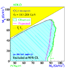
(a)

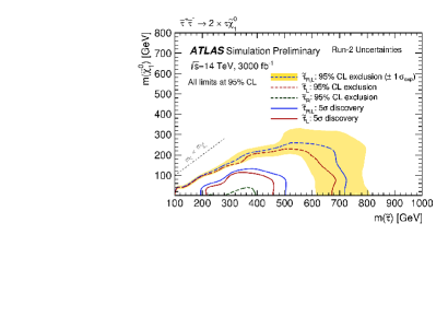
(b)

Figure 1: (a): 95$\%$ CL exclusion limits for $\widetilde{\tau}$ pair production obtained combining data collected at the four LEP experiments with energies ranging from 183 GeV to 208 GeV. From [8]. (b): 95$\%$ CL exclusion and discovery potential for $\widetilde{\tau}$ pair production at the HL-LHC, assuming $\widetilde{\tau}_{L}^{+}\widetilde{\tau}_{L}^{-}$ + $\widetilde{\tau}_{R}^{+}\widetilde{\tau}_{R}^{-}$ production, $\widetilde{\tau}_{L}^{+}\widetilde{\tau}_{L}^{-}$ production or $\widetilde{\tau}_{R}^{+}\widetilde{\tau}_{R}^{-}$ production. From [9].

An analysis by the DELPHI experiment, targeted at low mass differences, excludes a $\widetilde{\tau}$ with mass below 26.3 GeV, for any mixing, and any mass difference larger than the $\tau$ mass [10].

At the LHC, ATLAS and CMS have determined limits on the $\widetilde{\tau}$ mass, analysing data from Run 1 and Run 2 [11, 12]. These limits, however, are only valid under certain assumptions. Both experiments assume $\widetilde{\tau}_{R}$ and $\widetilde{\tau}_{L}$ to be mass-degenerate. This is a very unlikely scenario, the running of the $\widetilde{\tau}_{R}$ and $\widetilde{\tau}_{L}$ masses from the GUT scale to the weak scale follows renormalisation group equations with $\beta$-functions that are inevitably different for the two weak hyper-charge states. They also assume that there is no mixing between the weak hyper-charge eigenstates, which is again very improbable. The mixing will yield to cross section of the lightest physical state smaller than that of any unmixed state. Putting together $\widetilde{\tau}_{R}$ and $\widetilde{\tau}_{L}$ by adding the cross sections, ATLAS excludes $\widetilde{\tau}$ masses between approximately 120 and 390  GeV for a nearly mass-less neutralino. Under the same conditions, CMS extends the lower limit to 90  GeV closing the gap with the LEP limit. Analysis of a pure $\widetilde{\tau}_{L}$ pair production set limits between 150 and 310  GeV from ATLAS data and up to 125  GeV from CMS; both limits again assume a nearly mass-less neutralino.

The future HL-LHC should provide an improvement on the $\widetilde{\tau}$ limits provided by ATLAS and CMS, not only because of an increase of the luminosity but also because of an expected gain in sensitivity to direct $\widetilde{\tau}$ production due to the use of different analysis methods. Simulation studies have already been performed in both experiments [9, 13]. Upper limits for $\widetilde{\tau}$ masses are indeed increased by about 300  GeV, but they suffer from the same constraints as the previous studies. ATLAS adds limits for pure $\widetilde{\tau}_{R}$ pair production, that could be considered the closest case to the physical lightest $\widetilde{\tau}$ since it is likely to be the lightest of the two weak hyper-charge states and is the one with the lower cross section. These limits, presented in figure 1(b), show that no discovery potential is expected in this case, only exclusion potential. They do not have exclusion potential for $\widetilde{\tau}$ co-annihilation scenarios, a highly motivated scenario if SUSY is to provide a viable DM candidate: Such a scenario requires that the $\widetilde{\tau}$-LSP mass difference is small, $\lesssim$ 10 GeV.

$\widetilde{\tau}$ searches at the ILC have been also performed in previous studies [14]. They assume an integrated luminosity of 500  fb^-1 at $\sqrt{s}=500$ GeV and only used the $\mathcal{P}_{+-}$ data sample. In the current study, both $\mathcal{P}_{+-}$ and $\mathcal{P}_{-+}$ data are used, and the luminosity is increased to the one corresponding the the foreseen running scenario, 1.6  ab^-1 at each of the beam-polarisation combinations. The previous study was aimed at scanning the entire $M_{LSP}-M_{NLSP}$ plane, and doing so for several different NLSP candidates. Quite generic cuts were therefore used, and were optimised “on-the-fly” at different points. More specifically, the limits presented in that study do not have a dedicated analysis for low mass differences between the $\widetilde{\tau}$ and the LSP, $\Delta M$, and are only valid down to $\Delta M$ 3-4  GeV. The exclusion limit goes up to 240 GeV with a discovery potential up to 230 GeV for large mass differences.

A recent study of slepton production at ILC and, in general, future e+e- colliders can be found in [15]. They have demonstrated that these colliders would be able to probe most of the kinematically accessible parameter space with only a few days of data, with the capability of discovering/excluding new physics that would evade detection at the LHC.

5 Conditions and tools

The study was done assuming an integrated luminosity of 1.6  ab^-1 at $\sqrt{s}=500$ GeV for each of the beam polarisations $\mathcal{P}_{+-}$ and $\mathcal{P}_{-+}$, according to the H-20 running scenario for the ILC500 [16]. The study assumes R-parity conservation and a 100$\%$ decay of the $\widetilde{\tau}$ to ${\tau}$ and the lightest neutralino ($\chi^{0}_{1}$), the LSP in this case. In order to select the worst scenario, the $\widetilde{\tau}$ mixing angle was set to 53 degrees. This mixing angle corresponds to the lowest cross section in the case of un-polarised beams, due to the suppression of the s-channel with $Z$ exchange in the $\widetilde{\tau}$ pair production. In section 7.3, we will show that this mixing angle in fact also corresponds to the worst case at ILC operating according to the H20 scenario. The generated background event samples were those of the standard “IDR” production [17]. They were generated with Whizard 1.95 [18], and contain all standard model processes with up to six fermions in the final state. Beam-spectra and the amount of photons in the beams were simulated with GuineaPig [19]. Detector simulation and reconstruction were done on the Grid using DDSim [20] and Marlin [21]. The Grid production was done by the ILD production team using the Dirac [22] system. The SGV fast detector simulation [23], adapted to the ILD concept [17] at ILC, was used for detector simulation and event reconstruction for signal events. These events were generated with Whizard v2.8.5, interfaced to Tauola [24]. Tauola simulates the ${\tau}$-decays taking into account the ${\tau}$ polarisation in the products. The same beam-spectrum as was used for the fully simulated background samples was also used for the signal sample. Both the signal and background samples were analysed using the tools included in SGV, and the relevant information of the reconstructed events were written to Root files.

At ILC spurious events are expected to be present in each beam-crossing. At the ILC with $\sqrt{s}=500$ GeV an average of 1.5 low $\it{P_{T}}$ hadron events from $\gamma\gamma$ interactions is expected per bunch crossing. A number ($\mathcal{O}(10)$ ) of electron-positron pairs from beam-beam interactions is also expected to reach the tracking system of the detector in each bunch crossing. The $\gamma\gamma$ interactions were generated either with Pythia 6.422 [25] (if $M_{\gamma\gamma}$ > 2 GeV) or a dedicated generator [26] for $\gamma\gamma$ interactions (otherwise). The electron-positron pairs from beam-beam interactions were generated with GuineaPig. A pool of such events were created, and random events picked from the pool were added to each physics event during full simulation. The SGV simulation did not implement this mechanism, instead reconstructed objects coming from overlay were extracted from random background events and overlaid on the signal events at ntuple level.

Final significance values were computed adding the contribution of both polarisations. The signal production cross-section depends on the beam polarisation. Even more so, the background levels are expected to be quite different for the two cases, mainly because the strongly polarisation dependent $e^{+}e^{-}\rightarrow W^{+}W^{-}$ process is one of the most important sources of background. Because of this the samples are weighted by the likelihood ratio (LR) test statistic [27, 28]. As the experiment is a pure event-counting one, the LR statistic has the simple form

$$N_{\sigma}=\frac{\sum^{n_{samp}}_{i=1}s_{i}\ln{(1+s_{i}/b_{i})}}{\sqrt{\sum^{n_{samp}}_{i=1}n_{i}\left[\ln{(1+s_{i}/b_{i})}\right]^{2}}}$$ (1)

where $s_{i}$ and $b_{i}$ are expected number of signal and background events in each sample, and $N_{\sigma}$ is the significance of the test, expressed as the equivalent number of standard deviations in the Gaussian limit. Depending on which hypothesis is tested (exclusion or discovery), $n_{i}$ is either $s_{i}+b_{i}$ (exclusion), or $b_{i}$ (discovery).

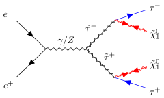
(a)

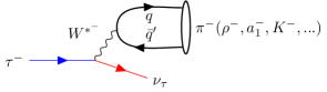
(b)

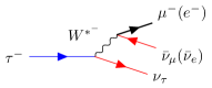
(c)

Figure 2: (a) $\widetilde{\tau}$ pair production and decay to $\tau$ and $\widetilde{\chi}^{0}_{1}$; (b) hadronic $\tau$ decay; (c) leptonic $\tau$ decay. Blue lines indicates the $\tau$, red lines indicate undetectable final state particles, while thick black lines indicate the detectable final state particles.

Well identifying $\tau$:s is obviously a key requirement for this analysis. To do this, we use the DELPHI $\tau$ finder  [10]. This algorithm was particularly developed to identify $\tau$:s in low multiplicity events. It iterative builds $\tau$ candidates from all possible combinations of charged tracks, starting with single tracks, then in each iteration adding tracks to existing combinations, always retaining the combination yielding the lowest mass, and requiring that the mass is below 2 GeV. Characteristics of $\tau$ decays are also taken into account, so that e.g. an identified muon is not allowed to be grouped with another track. The charged track grouping is terminated when no more groups with mass below 2 GeV can be made. Neutrals are then added to the found candidates, as long as the mass remains below 2 GeV - any neutrals that can not be grouped are left as belonging to the “rest-of-event” class. To allow for tracks not being found, it is not, at this stage, required that the groups have charge $\pm$ 1.

6 Signal and background

6.1 Signal characterisation

Assuming R-parity conservation and assuming that the $\widetilde{\tau}$ is the NLSP, $\widetilde{\tau}$’s will be produced in pairs via $Z^{0}$/$\gamma$ exchange in the s-channel and they will decay to a ${\tau}$ and an LSP (assuming mass differences above the mass of the ${\tau}$, as is done in this study). The LSP, as already mentioned, is stable and weakly interacting, hence it will leave the detector without being detected. The ${\tau}$, with a proper lifetime of 2.9 x 10^-13 s, will decay before leaving any signal in the detectors. The only detectable activity in the signal events is therefore the decay products of the two ${\tau}$’s. Figure 2(a) shows the diagram of the $\widetilde{\tau}$ production and decay, Figures 2(b) and (c) show the diagrams of the subsequent $\tau$ decays, in the hadronic and leptonic modes, respectively. Signal events are therefore characterised by a large missing energy and momentum, not only due to the invisible LSPs but also to the neutrinos from both ${\tau}$-decays. Since the $\widetilde{\tau}$’s are scalars and hence isotropically produced, these events have a large fraction of the detected activity in the central region of the detector.

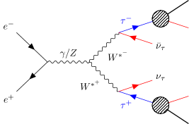
(a)

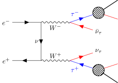
(b)

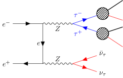
(c)

Figure 3: Main irreducible background sources: (a) s-channel $WW$ production with both $W$:s decaying to $\tau$ and $\nu$; (b) t-channel $WW$ production with both $W$:s decaying to $\tau$ and $\nu$; (c) t-channel $ZZ$ production with one $Z$ decaying to $\tau$:s, the other to $\nu$:s. The same colour-coding is as in Figure 2 is used, and the various $\tau$ decays modes (cf. Figures 2(b) and (c)) are collectively represented by the hatched circles.

The $\widetilde{\tau}$’s must also be rather heavy, so they will not have a large boost in the lab-frame, and since the LSP is also quite heavy, the direction of the $\widetilde{\tau}$ does not strongly correlate to that of the visible $\tau$ after the decay. As a consequence the two $\tau$-leptons are expected to go in directions quite independent of each other resulting in events with un-balanced transverse momentum, large angles between the two $\tau$-lepton directions and zero forward-backward asymmetry. These properties are however not necessarily present in any event - the two $\tau$’s could accidentally happen to be back to back, for example.

6.2 Main background sources

The main sources of background, given the generic signal topology, i.e. two $\tau$’s and an unseen recoil system, are SM processes with real or fake missing energy. They can be classified into “irreducible” and “almost irreducible” sources. The first are events with two $\tau$’s and real missing energy, i.e. neutrinos. The main contribution to this group are $ZZ$ events with one $Z$ decaying to two neutrinos and the other to two $\tau$’s, and fully leptonic $WW$ events, where both the $W$’s decays to $\tau$ and neutrino. The dominating diagrams are shown in Fig. 3. In principle, $ZWW$ and $ZZZ$ events decaying to two $\tau$’s and four neutrinos also contribute, but are of less concern due to their low cross sections. Nevertheless, these process are included in the simulated background samples.

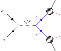
(a)

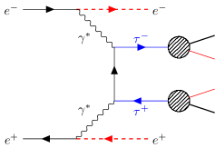
(b)

Figure 4: Main background sources: (a) $\tau$ pair production and decay; (b) $\tau$ pair production in $\gamma\gamma$ events. In (b), the thick dashed red lines indicate that while the outgoing electrons or positrons are in principle detectable, this diagram contributes to the background only in the case that they are deflected so little that they escape detection by remaining inside the beam-pipe, and hence contribute to (fake) missing energy.

The second group of events are those which are not really two $\tau$’s and neutrinos, but after reconstruction look very similar. They are events with two soft $\tau$-jets, with two other leptons plus true missing energy or two $\tau$’s plus fake missing energy. The main sources for events with true missing energy in this group are on one hand $\tau$ pair production, with the $\tau$’s decaying such that most energy goes to the neutrinos, (Figure 4(a)), and on the other hand, $ZZ$ or $WW$ decaying to two neutrinos and at least one lepton other than $\tau$’s, i.e. the type of processes shown in Figure 3, but with one, or both, $\tau$’s replaced by muons or electrons. The background with fake missing energy comes mainly from $\tau$ pair production with Initial State Radiation (ISR) at very low angles, events with two $\tau$’s and two very low angle electrons (below the acceptance of the detector) in the final state (Figure 4(b)) and events where two $\tau$’s are produced by a $\gamma\gamma$ interaction and not from an $e^{+}e^{-}$ one ; in the latter case there is not really missing energy but the assumption that the initial energy is the energy of the incoming electron and positron is wrong.

7 Analysis

7.1 General cuts

Taking into account the signal signature and the main background sources, different cuts have been designed in order to separate the signal from the background.

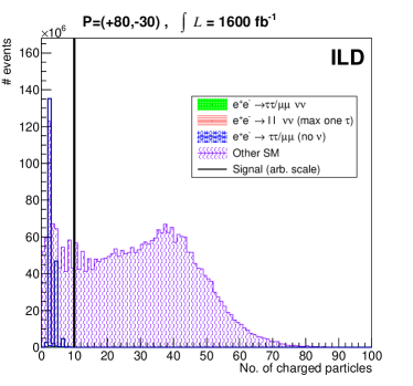
(a)

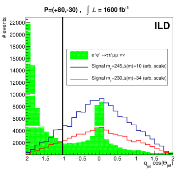
(b)

Figure 5: Distributions for background and signal (the latter on an arbitrary scale). (a): the number of charged particles. For clarity, the $\gamma\gamma$ background has been suppressed in this figure. (b) : $q_{jet}\cos{\theta_{jet}}$ after the cut on the number of charged particles. Only the irreducible $WW\rightarrow l\nu l\nu$ is shown, since this background is what this cut is designed to reduce. Events above the vertical lines are accepted.

The study was focused on small differences between the $\widetilde{\tau}$ and LSP masses, $M_{\tau}$ $<$ $\Delta M$ $<$ 11 GeV. This class of signal events are quite similar to high cross-section multi-peripheral $\gamma\gamma$ events, with one important difference, namely that in the $\gamma\gamma$ events the final state also includes the beam-remnant electrons and positrons. These are scattered by some low angle, so that demanding absence of signal in the calorimeter closest to the beam pipe (the BeamCal) strongly reduces this source of background, and was required as a pre-selection step before applying the following cuts. To reject tracks from low invariant mass $\gamma\gamma$ events and from beam-beam interactions (“overlay tracks”) occurring in the same bunch-crossing as the physics event, a selection of tracks is performed, details of which are given in Sect. 7.4.

All quantities mentioned in the following are to be understood as being calculated using reconstructed objects passing these cuts. Tables 2 and 3 show the cut-flow for the cuts applied at two model-points in the order the cuts are applied in the discussion that follows. All figures in this section will show background and signal distributions for various quantities that cuts are applied to at the point where the cut on the shown quantity will be the next one to be done, i.e. for events passing all previous cuts.

Initially, cuts are applied on properties that the signal often does not have, while some backgrounds do have: The multiplicity of the event can be constrained taking into account that the visible part of the $\widetilde{\tau}$ decays comes only from the decays of the two $\tau$’s and maybe an ISR photon. For that reason the number of charged particles in the event is required to be between 2 and 10. This cut removes practically all hadronic background, see Fig. 5(a). $WW$ events with each of the $W$’s decaying to a lepton and a neutrino are highly forward-backward asymmetric; they can be effectively removed by requiring the sum of the product of the charge and the cosine of the polar angle, $q\cos{\theta_{jet}}$, of the two most energetic jets to be above -1.0, see Fig. 5(b). $ZZ$ events with one $Z$ decaying to two neutrinos and the second one to a electron or muon pair are highly suppressed demanding $|M_{vis}-M_{Z}|>4$ GeV, see Fig. 6 (a).

The cuts mentioned in the previous paragraph does not depend on the properties of the signal model point. However, all following cuts applied will depend on the model-point considered, and so will depend on either, or both, of $M_{\widetilde{\tau}}$ and $M_{LSP}$.

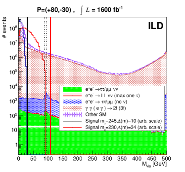
(a)

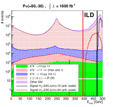
(b)

Figure 6: Distributions of the visible mass (a) and the missing energy (b), for two signals (arbitrary scale), and background, after previous cuts have been applied (cf. Tabs. 2 and 3). Events below (above) the vertical lines are accepted in a(b) at the model points indicated by the colour of the lines. In the $M_{vis}$ distribution, also events between the dashed lines around $M_{Z}$ were rejected.

The first group of cuts contain those in properties that the $\widetilde{\tau}$-events must have. Since the two LSPs from the $\widetilde{\tau}$-decays are invisible to the detector, signal events have to have a missing energy, $E_{miss}$, greater than $2\times M_{LSP}$.

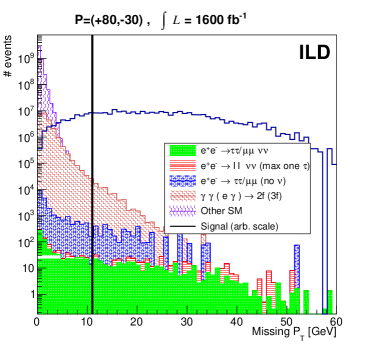
(a)

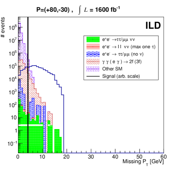
(b)

Figure 7: Distributions of the missing transverse momentum for (a) M${}_{\widetilde{\tau}}$ = 230 GeV $\Delta(M)$ = 34 GeV, and (b) M${}_{\widetilde{\tau}}$ = 245 GeV $\Delta(M)$ = 10 GeV. The two signals are on arbitrary scale, and all previous cuts have been applied (cf. Tabs. 2 and 3). Events above the vertical lines are accepted.

Likewise, the visible mass, $M_{vis}$ can not be greater than $E_{CMS}-2\times M_{LSP}$. Therefore, events should fulfil $M_{vis}<E_{CMS}-2\times M_{LSP}$ (Fig. 6 (a)) and $E_{miss}>2\times M_{LSP}$ (Fig. 6 (b)) to be considered further. Also a cut in the maximum total momentum, smaller than 70$\%$ the beam momentum, is applied for the same reason: $P_{tot}<0.70E_{beam}$. There should only be 2 or 3 clusters found by the Jade algorithm (with $y_{cut}$=0.02) and a total seen event charge should be between -1 and 1. A specific algorithm for $\tau$-identification was also applied. This algorithm consists in a first set of conditions requiring to have a pattern of charged tracks typical for $\tau$-decay, viz. exactly two $\tau$-jets (obtained with the DELPHI tau-finder) with 1 or 3 charged particles in each charged jet, jet-charge $\pm$1, and opposite charge between both jets. These two jets could be accompanied by further particles, that are not compatible with the requirements imposed by the DELPHI tau-finder to be considered as $\tau$-jets. A further set of conditions on the jets is devoted to the reduction of background from sources with leptons not from $\tau$-decays. The background of single $W$, with the $W$ decaying to $\tau$ and neutrino, see Figure 8, can be reduced by a cut depending on beam-polarisation: this process can only occur if at least one of the beams has the correct polarisation. Since the degree of polarisation of the positron beam is lower than that of the electron beam, this background is more likely to yield an electron as the beam-remnant for $\mathcal{P}_{+-}$, a positron for $\mathcal{P}_{-+}$. We therefore remove events with an electron(positron) $\tau$ candidate in the $\mathcal{P}_{+-}$ ( $\mathcal{P}_{-+}$) samples.

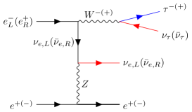
Figure 8: Single $W$ production with the $W$ decaying to $\tau$ and $\nu$. The labels indicate the only beam-polarisations for which this process is possible: either left-handed electrons or right-handed positrons.

This background together with the background from $WW\rightarrow e\nu_{e}\mu\nu_{\mu}$ and from $\gamma\gamma$ events with a beam-remnant deflected to larger angles is further reduced by rejecting those events in which the most energetic jet consists of a single electron. The two charged jets were also required to not be made by single leptons with the same flavour. These selections reduce the signal efficiency to 38$\%$ but with a reduction of the background of the order of 94$\%$, depending on the region of the SUSY parameter space.

Since the $\widetilde{\tau}$-decay is a two body decay, it is possible to determine the maximum and minimum momentum of each of the decay products as a function of the $\widetilde{\tau}$ mass, the mass of LSP and the centre-of-mass energy of the collider. A cut in the minimum momentum can not be applied due to the presence of neutrinos in the $\tau$ decay, with the corresponding decrease of observable momentum. The maximum value can be used even if it is smeared by the missed neutrinos. The expression for the maximum jet momentum is given by:

$$P_{max}=\frac{\sqrt{s}}{4}\left(1-\left(\frac{M_{LSP}}{M_{\widetilde{\tau}}}\right)^{2}\right)\left(1+\sqrt{1-\frac{4M_{\widetilde{\tau}}\leavevmode\nobreak\ ^{2}}{s}}\right)$$ (2)

and events with the higher jet momentum above this limit are excluded from the further analysis at the given model point. Excluding the cut applied by the $\tau$-identification algorithm, the signal efficiency for each of the cuts is at least 95$\%$ at all model points.

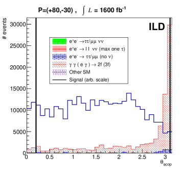
(a)

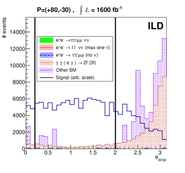
(b)

Figure 9: Distributions of the acoplanarity angle between the two jets for (a) M${}_{\widetilde{\tau}}$ = 230 GeV $\Delta(M)$ = 34 GeV, and (b) M${}_{\widetilde{\tau}}$ = 245 GeV $\Delta(M)$ = 10 GeV. The two signals are on arbitrary scale, and all previous cuts have been applied (cf. Tabs. 2 and 3). Events between the vertical lines are accepted.

A second group of cuts is based on those properties that the $\widetilde{\tau}$-events might have, but will rarely be

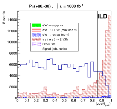
(a)

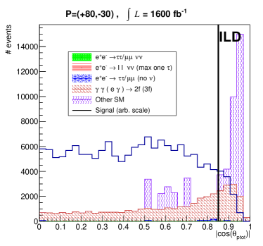
(b)

Figure 10: Distributions of the polar angle of the vectorial sum of the two jet momenta for (a) M${}_{\widetilde{\tau}}$ = 230 GeV $\Delta(M)$ = 34 GeV, and (b) M${}_{\widetilde{\tau}}$ = 245 GeV $\Delta(M)$ = 10 GeV. The two signals are on arbitrary scale, and all previous cuts have been applied (cf. Tabs. 2 and 3). Events below the vertical lines are accepted.

present in background events. As already pointed out, the $\widetilde{\tau}$’s are scalars, and therefore isotropically produced, while the backgrounds are either fermions or vector bosons, and tend to be produced at small angles to the beam axis. This allows to impose cuts requiring events to have high missing transverse momentum ($P_{Tmiss}$), and large acoplanarity $\theta_{acop}$. The distributions for these two quantities are shown in Figs. 7 and 9, for two model-points as they are after applying all previous cuts, applicable to the model-points in question. The total seen momentum, $\sum\bar{p}$, tends to be in an almost random direction in signal events, while it tends to point close to the beam-axis for most backgrounds. Therefore a cut on the direction of the total momentum, $|\cos(\theta_{\sum\bar{p}})|<0.85$, was imposed, see Fig.10. In addition, a cut on the variable $\rho$ is imposed. This variable is calculated by first projecting the event on the x-y (transverse) plane, and calculating the thrust axis in that plane. $\rho$ is then the transverse momentum (in the plane) with respect to the thrust axis. The cut in $\rho$ helps to reject events with two $\tau$’s back-to-back in the transverse projection with the visible part of the decay of one of the $\tau$’s in the direction of its parent, while the other $\tau$ decays with the invisible $\nu$ closely aligned with the direction of its parent. These events fake the signal topology, having both a large missing transverse momentum and high acoplanarity. However, they would have a small value of $\rho$. The distributions of $\rho$ for signal and background, at this point in the cut chain, are shown in Fig. 11, for two model points. The values at which the cuts described in this paragraph are set depends on the mass difference between the $\widetilde{\tau}$ and the LSP (except the cut on $\theta_{\sum\bar{p}}$), and are detailed in Tab. 1.

Table 1: Cuts depending on the mass difference between the $\widetilde{\tau}$ and the LSP. The specific cuts applied for $\Delta(M)$ = 2 GeV are explained in Sect. 7.2.

$\Delta(M)$	$P_{Tmiss}$	$\rho$	$\theta_{acop}$
[GeV]	[GeV]	[GeV]	[Rad]
34	$>$ 11	$>$ 11	$\in[0.2,3.1]$
10	$>$ 4	$>$ 8	$\in[0.2,2.0]$
3	$>$ 2	$>$ 3	$\in[0.2,2.3]$
2	-	no cut	$\in[0.2,2.3]$

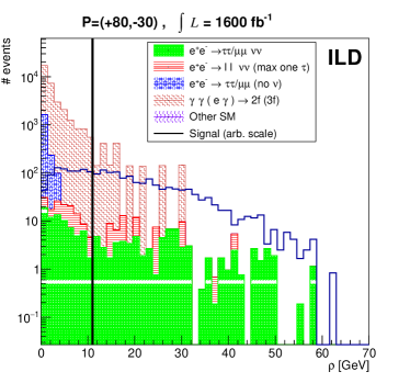
(a)

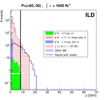
(b)

Figure 11: Distributions of the variable $\rho$, described in the text, for (a) M${}_{\widetilde{\tau}}$ = 230 GeV $\Delta(M)$ = 34 GeV, and (b) M${}_{\widetilde{\tau}}$ = 245 GeV $\Delta(M)$ = 10 GeV. The two signals are on arbitrary scale, and all previous cuts have been applied (cf. Tabs. 2 and 3). Events above the vertical lines are accepted.

Cutting in these properties has a certain cost in efficiency but improves the signal-to-background ratio.

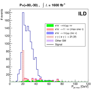
(a)

Figure 12: Distribution of the higher of the two jet momenta after all cuts (except the one on $p_{jet\leavevmode\nobreak\ max}$ itself) corresponding to the model point M${}_{\widetilde{\tau}}$ = 230 GeV, $\Delta(M)$ = 34 GeV. The maximum $P_{jet}$ possible at this model point is 47.63 GeV (Eq. 2), and is indeed the endpoint of the signal distribution. (Contrary to other figures in this section, the signal is stacked on top of the background, and corresponds to the same integrated luminosity as the background.)

As a final cut it is noted that sizeable energy detected at low angles to the beam is rare in signal events, but common in many backgrounds. Events with more than 2 GeV detected at angles lower than 20 degrees to the beam axis are therefore rejected. This cut is however not useful for small mass differences. After applying these cuts the main sources of remaining background are $WW$ events with each $W$ decaying to $\tau\nu$ and events with four fermions in the final state coming from $\gamma\gamma$ interactions, mostly $\tau\tau$ events. As an illustration of the expected signal after all cuts, Fig 12 shows the distribution of the higher of the two jet-momenta ($p_{jet\leavevmode\nobreak\ max}$) for the model-point with M${}_{\widetilde{\tau}}$ = 230 GeV and $\Delta(M)$ = 34 GeV, when all described cuts except the one on $p_{jet\leavevmode\nobreak\ max}$ has been applied. In this figure, the signal and background distributions correspond to the same 1600 fb^-1 of integrated luminosity.

Table 2: Flow table M${}_{\widetilde{\tau}}$ = 230 GeV $\Delta(M)$ = 34 GeV. The numbers correspond to an integrated luminosity of 1.6 ab^-1 and polarisation $\mathcal{P}_{+-}$.

Cut	Signal	$e^{+}e^{-}\rightarrow$	$e^{+}e^{-}\rightarrow$	$e^{+}e^{-}\rightarrow$	$\gamma\gamma(\gamma e)\rightarrow$	All other
		$\tau\tau/\mu\mu\leavevmode\nobreak\ \nu\nu$	$ll\leavevmode\nobreak\ \nu\nu$	$\tau\tau/\mu\mu$	2(3) fermions
			($\geq 1\leavevmode\nobreak\ l$ not $\tau$)	(no $\nu$’s)
no cut	$8292.8$	$134\,100$	$533\,900$	4.377 $\cdot 10^{6}$	1234 $\cdot 10^{6}$	2616 $\cdot 10^{6}$
BeamCal veto	$8284.5$	$133\,966$	$532\,800$	4.368 $\cdot 10^{6}$	1086 $\cdot 10^{6}$	2603 $\cdot 10^{6}$
2 $\leq N_{charged}\leq$ 10	$8219.0$	$108\,900$	$403\,100$	3.542 $\cdot 10^{6}$	1024 $\cdot 10^{6}$	1720 $\cdot 10^{6}$
$q\cos{\theta_{jet}}>-1$	$7179.1$	$70\,720$	$216\,800$	2.671 $\cdot 10^{6}$	841.6 $\cdot 10^{6}$	1504 $\cdot 10^{6}$
$|M_{vis}-M_{Z}|>4$	$7178.2$	$66\,820$	$207\,200$	2.552 $\cdot 10^{6}$	826.8 $\cdot 10^{6}$	1500 $\cdot 10^{6}$
$E_{miss}>2M_{LSP}$	$7177.4$	$19\,620$	$14\,570$	$365\,493.0$	238.0 $\cdot 10^{6}$	1399 $\cdot 10^{6}$
$M_{vis}<\sqrt{s}-2M_{LSP}$	$7103.6$	$17\,990$	$12\,490$	$334\,886.7$	235.5 $\cdot 10^{6}$	1398 $\cdot 10^{6}$
$\tau$ Id	$2953.9$	$1250$	$451.2$	$29\,088.3$	23.96 $\cdot 10^{6}$	166.9$\cdot 10^{6}$
$P_{jet}<P_{max}$	$2953.9$	$1003$	$268.3$	$23\,963.2$	23.55 $\cdot 10^{6}$	165.6$\cdot 10^{6}$
$P_{Tmiss}$ > 11 GeV	$2478.7$	$242.5$	$175.6$	$3481$	$83\,970$	$54.7$
$\theta_{acop}\in$ [0.2, 3.1]	$2293.8$	$208.6$	$144.9$	$3075$	$69\,190$	$52.0$
$|\cos(\theta_{\sum\bar{p}})|<0.85$	$2125.4$	$147.1$	$113.6$	$1876$	$32\,520$	$39.8$
$\rho$ > 11	$1317.7$	$60.3$	$39.3$	$0.0$	$1923$	$19.3$
$E_{<20^{\circ}}<2$ GeV	$1015.9$	$39.6$	$27.2$	$0.0$	$81.0$	$12.1$

Table 3: Flow table M${}_{\widetilde{\tau}}$ = 245 GeV $\Delta(M)$ = 10 GeV. The numbers correspond to an integrated luminosity of 1.6 ab^-1 and polarisation $\mathcal{P}_{+-}$.

Cut	Signal	$e^{+}e^{-}\rightarrow$	$e^{+}e^{-}\rightarrow$	$e^{+}e^{-}\rightarrow$	$\gamma\gamma(\gamma e)\rightarrow$	All other
		$\tau\tau/\mu\mu\leavevmode\nobreak\ \nu\nu$	$ll\leavevmode\nobreak\ \nu\nu$	$\tau\tau/\mu\mu$	2(3) fermions
			($\geq 1\leavevmode\nobreak\ l$ not $\tau$)	(no $\nu$’s)
no cut	$672.8$	$134\,100$	$533\,900$	4.377 $\cdot 10^{6}$	1234 $\cdot 10^{6}$	2616 $\cdot 10^{6}$
BeamCal veto	$672.1$	$133\,966$	$532\,800$	4.368 $\cdot 10^{6}$	1086 $\cdot 10^{6}$	2603 $\cdot 10^{6}$
2 $\leq N_{charged}\leq$ 10	$664.3$	$106\,400$	$403\,100$	3.542 $\cdot 10^{6}$	1024 $\cdot 10^{6}$	1720 $\cdot 10^{6}$
$q\cos{\theta_{jet}}>-1$	$585.2$	$70\,720$	$216\,800$	2.671 $\cdot 10^{6}$	841.7 $\cdot 10^{6}$	1504 $\cdot 10^{6}$
$|M_{vis}-M_{Z}|>4$	$585.2$	$66\,820$	$207\,200$	2.552 $\cdot 10^{6}$	826.8 $\cdot 10^{6}$	1500 $\cdot 10^{6}$
$E_{miss}>2M_{LSP}$	$585.1$	$6218$	$886.6$	$120\,800$	179.0 $\cdot 10^{6}$	1043 $\cdot 10^{6}$
$M_{vis}<\sqrt{s}-2M_{LSP}$	$583.9$	$5669$	$758.0$	$109\,100$	172.7 $\cdot 10^{6}$	969.9 $\cdot 10^{6}$
$\tau$ Id	$230.6$	$484.0$	$56.3$	$13\,020$	1.010 $\cdot 10^{6}$	127.4 $\cdot 10^{6}$
$P_{jet}<P_{max}$	$229.9$	$444.2$	$38.2$	$11\,150$	$822\,400$	108.0 $\cdot 10^{6}$
$P_{Tmiss}$ > 4 GeV	$177.4$	$33.4$	$5.1$	$435.0$	$36\,210$	$84\,660$
$\theta_{acop}\in$ [0.2, 2.0]	$164.6$	$30.0$	$5.1$	$299.6$	$32\,310$	$71\,650$
$|\cos(\theta_{\sum\bar{p}})|<0.85$	$156.4$	$22.7$	$0.0$	$290.0$	$24\,220$	$20\,290$
$\rho$ > 8	$55.6$	$2.7$	$0.0$	$0.0$	$798.6$	$0.5$
$E_{<20^{\circ}}<2$ GeV	$55.6$	$2.7$	$0.0$	$0.0$	$610.2$	$0.5$

The polarisation plays an important role in the capability of excluding/discovering the different regions of the SUSY space. Table 4 shows the number of signal and background events for a specific model point for the two main ILC running polarisations and for unpolarised beams. The difference in the number of signal events arises from the dependence of the cross section on the polarisation, as well as from the effect on selection efficiency due to the polarisation of the $\tau$ coming from the $\widetilde{\tau}$. The dependence of the cross section on the polarisation is the main factor for the difference in $WW$ events, $e^{+}e^{-}\rightarrow\tau\nu\tau\nu$. One can see that the signal-to-background ratio is clearly enhanced for the case of mainly right-handed electrons, left-handed positrons. Taking the definition of exclusion at 95$\%$ CL as $N_{\sigma}>2$ (cf. Eq. 1), it can be seen that combining the two polarisation samples with the LR statistic does strengthen the limit, even though the $\mathcal{P}_{-+}$ sample gives a much weaker limit than the $\mathcal{P}_{+-}$ one. It is also shown that unpolarised beams would allow neither exclusion nor discovery, even though the sample corresponds to the same integrated luminosity as the sum of the two polarised samples. This is not only because of the possibility to combine samples with different beam polarisations in an optimal way is not available for unpolarised beams; it is also because the ILC has both beams polarised, meaning that more than half of the collisions are between opposite polarised particles, which is necessary to allow for s-channel processes, such as $\widetilde{\tau}$ pair production. Polarisation is not only important in the enhancement of the signal over background but also plays an important role in the parameter determination.

Table 4: Remaining signal and background events after the application of the selection cuts for $M_{\widetilde{\tau}}$=245  GeV and mass difference with the LSP of 10  GeV.

Polarisation	Signal	$e^{+}e^{-}\rightarrow$	$\gamma\gamma(\gamma e)\rightarrow$	All other	Nσ
		$\tau\tau/\mu\mu\leavevmode\nobreak\ \nu\nu$	2(3) fermions
$\mathcal{P}_{+-}$	$55.6$	$2.7$	$610.2$	$0.5$	$2.1$
$\mathcal{P}_{-+}$	$36.0$	$39.6$	$1208$	$0.5$	$1.0$
Combined	-	-	-	-	$2.4$
Unpolarised	$73.9$	$34.1$	$1818$	$1.0$	$1.7$

7.2 Low $\Delta(M)$ cuts

The cuts described above are suited for mass differences down to 3  GeV. When the mass difference is between 3  GeV and the mass of the $\tau$ the kinematics of the signal events is very close to that of the $\gamma\gamma$ background events and the described cuts are not enough for discovering/excluding the signal. An additional cut was done based on the Initial State Radiation photons (ISR). Events with isolated photons with sizeable energy were selected, allowing to extension of the limits into the region under study. To select these, the photon should be at above 7^∘ to the beam - the lower edge of the acceptance of the tracking system of ILD - to avoid that electrons would be mistaken for photons, and it should have an energy above 1.1 GeV.

This cut is effective against the remaining $\gamma\gamma$ background because these events become candidates due to fake missing transverse momentum. If the presence of an ISR is requested, the incoming electron or positron that emitted the ISR must have recoiled against the ISR. Since this is a scattering process, not an annihilation one, the electron (positron) is still present in the final state. Therefore, if it is required to see a high transverse momentum ISR, the final state electron (positron) will have acquired a recoil transverse momentum big enough to be deflected into the BeamCal, and thus to have been rejected already at the pre-selection stage. On the other hand, if the ISR was emitted from an electron or positron that was subsequently annihilated into a $Z$, as is the case for the signal process, the transverse momentum of the ISR is included in the decay products of the $Z$, and no signal is expected in the BeamCal.

Events containing such ISR photons, and passing all cuts except those detailed in Tab. 1, were retained if $P_{Tmiss}>4$ GeV and the sum of the absolute value of the jet momenta was between 1 and 4 GeV.

7.3 Determining the worst scenario

The aim of this study is to evaluate the capabilities of the $\widetilde{\tau}$ search at ILC with no loopholes. One of the properties of the $\widetilde{\tau}$ - apart from its and the LSP masses - is the $\widetilde{\tau}$ mixing. This enters in two ways: The production cross-section depends on it, as does the polarisation of the $\tau$. The dependence of the cross-section on the $\widetilde{\tau}$ mixing angle is shown in Fig. 13, for the two beam-polarisations considered at ILC. Also shown is dependence for unpolarised beams, which shows a minimum at 53^∘. The polarisation of the $\tau$ is also important, since it influences the momentum distribution of the ${\tau}$-decay products, and hence the signal efficiency: if the $\tau$ is pre-dominantly left-handed, and since there are no right-handed neutrinos in the standard model, the invisible neutrino will tend to align with the direction of the $\tau$ and take a larger fraction of the momentum, and consequently the visible system will take less. This is illustrated in Fig.  14 which shows the momentum distribution of the pions coming from ${\tau}$-decays (in the single pion decay mode) for different $\widetilde{\tau}$ mixing angles and a bino-LSP. The ${\tau}$ polarisation from the $\widetilde{\tau}$ decay depends not only on the $\widetilde{\tau}$ but also on the neutralino mixing angle. This is because of the different behaviour of the interaction between higgsinos and binos with the $\widetilde{\tau}$. The higgsino (like the Higgs) carries weak hyper-charge, while the bino (like the $Z$ or the photon) does not. Therefore, with a higgsino LSP, the $\widetilde{\tau}$ produces a ${\tau}$ with the opposite chirality with respect to that of the $\widetilde{\tau}$, while with a bino LSP, the produced ${\tau}$ has the same chirality. Since the lowest efficiency is expected for left-handed $\tau$’s, we evaluate the efficiency for the assumption that the neutralino is a pure Bino for $\widetilde{\tau}$ mixings below 45^∘ (i.e. for a $\widetilde{\tau}$ more left than right), and for a pure higgsino LSP for mixings above 45^∘. This assures that the most difficult case is studied at any mixing. In Fig. 15(a) the signal efficiency for an example point is shown, with these assumptions.

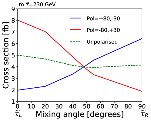
Figure 13: Cross section for $\widetilde{\tau}$ pair production as a function of the $\widetilde{\tau}$ mixing angle for the two main ILC polarisations. The green dotted line shows the case corresponding to the simply combination of both samples, corresponding to unpolarised beams for equal integrated luminosity.

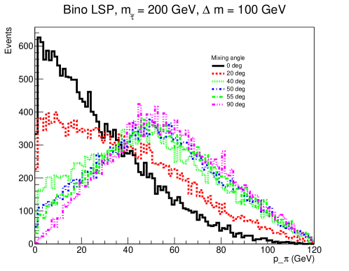
Figure 14: Momentum distribution of the pions coming from ${\tau}$-decays in the mode $\tau\rightarrow\pi^{\pm}\nu$ for different $\widetilde{\tau}$ mixing angles. The neutralino was assumed to be a pure bino.

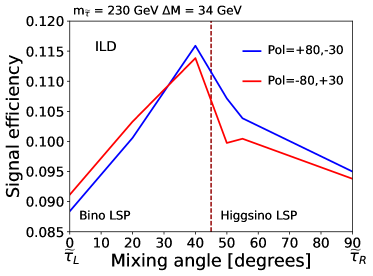
(a)

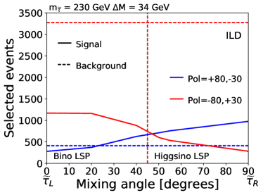
(b)

Figure 15: (a): Signal efficiency as a function of the $\widetilde{\tau}$ mixing angle for both main ILC polarisations. The LSP composition was chosen giving the worst case for each mixing. (b):Number of signal and background selected events as a function of the $\widetilde{\tau}$ mixing angle for both main ILC polarisations.

Combining cross sections and signal efficiencies, the number of selected signal events for each polarisation as a function of the $\widetilde{\tau}$ mixing angle was evaluated. Figure 15(b) shows the obtained values together with the number of background events passing the selection cuts, which is different for each beam polarisation but obviously do not have any dependence on the $\widetilde{\tau}$ mixing angle. As can be seen, the background is much larger for the $\mathcal{P}_{-+}$ sample. This is because the irreducible background from $e^{+}e^{-}\rightarrow WW\rightarrow\tau\nu\tau\nu$ is strongly polarisation dependent. This constitutes the final ingredient to estimate the worst-case scenario: from these values, the signal over background significance as a function of the mixing angle was computed for each polarisation, as shown in figure 16(a). Final significance values were computed adding the contribution of both polarisations weighted by the likelihood ratio statistic. The results are plotted in figure 16(b). One can see that rather uniform sensitivity to all mixing angles is obtained, and that for the smallest mass differences - the ones closest to the critical region - a mixing angle around 53^∘ can indeed be considered as the worst one, and validates our choice of this mixing angle being the worst case.

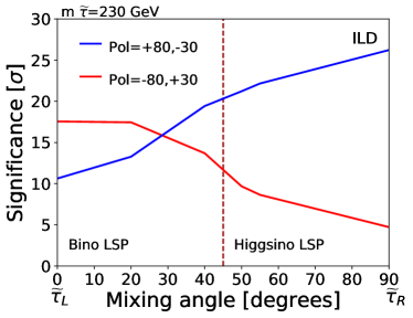
(a)

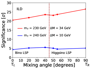
(b)

Figure 16: (a): Signal significance as a function of the $\widetilde{\tau}$ mixing angle for both main ILC polarisations. (b)Signal significance weighting both polarisations using the likelihood-ratio static in the H20 ILC conditions.

7.4 Effect of overlay tracks

The overlay tracks can not be neglected in the $\widetilde{\tau}$ studies, since they have similar properties to the visible tracks from the $\widetilde{\tau}$-decays in the region with small mass differences between $\widetilde{\tau}$ and LSP. The main characteristics of the overlay tracks are the low transverse momentum and low angles to the beam axis. The tracks in low $\it{P_{T}}$ hadron events usually originates in the beam-spot, contrary to the tracks from the $\tau$ decays. Figure 17(a) compares transverse momentum distributions for signal and overlay tracks, and it can be seen that while the overlay tracks can easily be removed by a cut in this quantity for large to moderate mass-differences, this is not possibly for the smallest ones. Figure 17(b) makes the same comparison for the cosine of the polar angle of the tracks, showing that in this variable, the difference between overlay and signal tracks does not depend on the mass-difference.

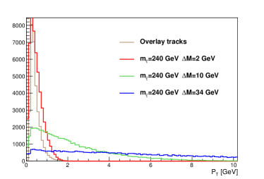
(a)

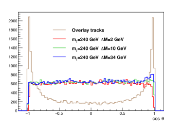
(b)

Figure 17: (a): Transverse momentum distribution for signal and overlay tracks. Signal tracks correspond to different mass differences between $\widetilde{\tau}$ and LSP. (b): Distribution of cosine of polar angle for signal and overlay tracks. Signal tracks correspond to different mass differences between $\widetilde{\tau}$ and LSP.

In the type of event-topologies the signal gives rise to, viz. two displaced $\tau$ decays, no primary vertex can be fitted. However, at ILC the transverse beam-spot size is significantly smaller than the measurement precision, so that in that plane, the primary vertex position is known, even without fitting. The longitudinal size of the beam-spot, on the other hand, is much larger than the measurement precision. Figure 18 shows the significance of the impact parameter with respect to the origin in the transverse direction for overlay and signal tracks for different mass differences. Here, the impact parameter has been life-time signed, i.e. the sign is determined by the position w.r.t. to the beam-spot where the track intersects the axis of the jet it belongs to, taking the direction of the jet as the positive direction. For the overlay tracks, the expected insignificant transverse impact parameters for tracks originating inside the beam-spot is observed. For the signal case, one observes more and more significant deviation in the impact parameters, reflecting that the tracks do not originate from inside the beam-spot.

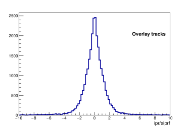
(a) overlay

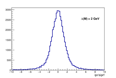
(b) $\Delta(M)$ = 2 GeV

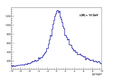
(c) $\Delta(M)$ = 10 GeV

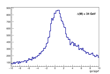
(d) $\Delta(M)$ = 34 GeV

Figure 18: Transverse impact parameter significance of tracks from overlay and from signals with $M_{\widetilde{\tau}}$ = 240 GeV, and different mass-differences.

Hence, for model points with mass differences $\leq$ 10 GeV, we select tracks with $|cos{\theta}|<0.7$, and the transverse impact parameter significance larger than 2. If the mass difference is $>$ 10 GeV, we instead require that. $P_{T}>2$ GeV.

While these cuts clearly occasionally will remove tracks from the $\tau$ decay resulting in the event being lost as a candidate (since the strict topology requirements of exactly two $\tau$-jets with the correct charges will not be met), this is compensated by previous lost candidates being salvaged by removing wrongly included tracks from overlay in the topology evaluation. This, together with the fact that many background events only became candidates because of the presence of overlay tracks, and so will be discarded by the cuts, results in a net amelioration of the sensitivity. Figure 19 shows the results obtained with and without cuts together with the results obtained if the overlay tracks were added neither to signal nor background. For the case with the smallest mass difference, shown in Figure 19(a), there is a strong reduction of the significance when adding overlay tracks. For the larger mass-difference (Figure 19(b)), there is only a slight degradation due to the overlay tracks. For both mass differences, the overlay removal procedure indeed ameliorates the sensitivity.

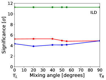
(a) $\Delta(M)=$ 3 GeV

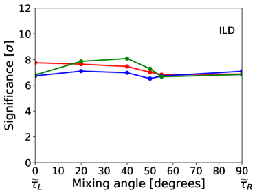
(b) $\Delta(M)=$ 10 GeV

Figure 19: Number of sigmas for a $\widetilde{\tau}$ with mass 240 GeV and different mass-differences. The plot assumes H20 ILC scenario combining both polarisations using the likelihood-ratio statistic. Blue lines correspond to the case with all the tracks and the red ones after rejecting tracks not satisfying the cuts described in the text. The green curves correspond to the study without overlay tracks.

8 Exclusion/discovery limits

The exclusion and discovery limits extracted from this study are shown in Figure 20. They assume the lightest $\widetilde{\tau}$ to be the NLSP and the lightest neutralino the LSP, and are valid for any $\widetilde{\tau}$ mixing angle. It is also relevant to compare these results with the current $\widetilde{\tau}$ limits coming from LEP. The LEP limits are also valid for any value of the not shown model parameters.

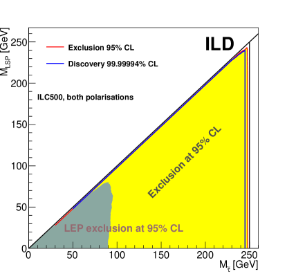
Figure 20: Exclusion and discovery $\widetilde{\tau}$ limits from the current studies compared to the ones from LEP studies [8]. The ILC region corresponds to the full H20 data-set at $E_{CMS}$ = 500 GeV, i.e. 1.6 ab^-1 at each of the beam polarisations $\mathcal{P}_{+-}$ and $\mathcal{P}_{-+}$.

The projection of the limits in the $M_{\widetilde{\tau}}$-$\Delta$M plane is shown in figure 21. The region for mass differences below the mass of the $\tau$, not included in the current study, is shown for completeness. In the region with $\Delta$M larger than $M_{\tau}$ exclusion and discovery ILC limits are compared to the ones from LEP. The projected HL-LHC limits are also shown. Since they are highly model-dependent, the comparison in this case have to be taken with care: here limits considering only the $\widetilde{\tau}_{R}$-pair production are shown, since, while still being optimistic, they are closest to the ones expected for the lightest $\widetilde{\tau}$ at minimal cross-section. It should be noted that the HL-LHC projection is only an exclusion limit - no discovery potential is expected.

For the region with $\Delta$M smaller than $M_{\tau}$ results from LEP and LHC are shown. The LEP studies cover not only the region where the $\widetilde{\tau}_{1}$ travels through the detector without decaying but also the region with decays at a certain distance from the production vertex. In those regions acoplanar leptons, tracks with large impact parameters and kinked tracks are looked for, depending on the $\widetilde{\tau}_{1}$ lifetime [29, 30]. The figure also shows the extrapolation of the ILC limits for the scenarios with centre-of-mass energy 250  GeV and 1  TeV.

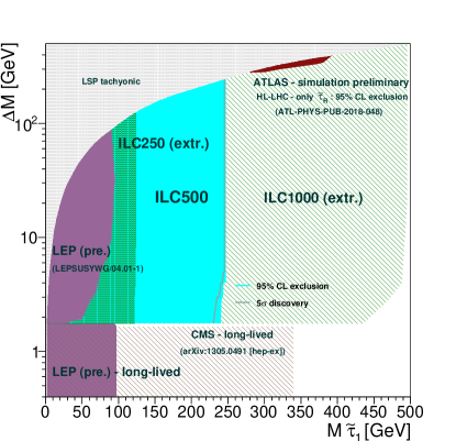
Figure 21: $\widetilde{\tau}$ limits in the $M_{\widetilde{\tau}}$-$\Delta$M plane. ILC results from the current studies are shown together with limits from LEP [8] and projection for HL-LHC [9]. The ILC region corresponds to the full H20 data-set at $E_{CMS}$ = 500 GeV, i.e. 1.6 ab^-1 at each of the beam polarisations $\mathcal{P}_{+-}$ and $\mathcal{P}_{-+}$. The region with mass differences below the mass of the ${\tau}$ is also shown with LEP  [29, 30] and LHC results [31], even if it is not covered by this study. In addition, the extrapolation of the ILC current results to the ILC 250  GeV and 1  TeV running scenarios is shown.

8.1 Comparison with previous study

Results from previous ILC studies, which used a $\int\mathcal{L}$dt = 500  fb^-1 sample of events with beam polarisation $\mathcal{P}_{+-}$ are shown in Figure  22, together with results obtained under those conditions with the present analysis.

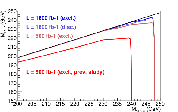
Figure 22: Exclusion and discovery $\widetilde{\tau}$ limits as a function of the $\widetilde{\tau}$ and LSP masses. Exclusion limits from previous ILC studies [14] are also shown, as well as the current analysis applied to the same data-sample as the previous one, i.e. only the $\mathcal{P}_{+-}$ beam polarisation sample.

The comparison of these two curves shows that the extension of the limits is not only due to an increase of the total integrated luminosity but also to an improvement of the analysis. The main reason of this improvement is the application of individual limits depending on the $\widetilde{\tau}$ mass and the mass difference. The previous studies were only making a difference for mass differences above or below 10  GeV and were not optimised for the low mass difference region. Another difference in the analysis is a change in the ${\tau}$-identification algorithm, excluding events with two jets consisting of single leptons of the same flavour.

9 Outlook and conclusions

The capability of the ILC for excluding/discovering $\widetilde{\tau}$-pair production up to a few GeV below the kinematic limit, without model dependencies and even in the worst scenario, has been shown.

The worst scenario for $\widetilde{\tau}$-pair production at the ILC was reviewed taking into account ILC beam polarisation conditions. Equal sharing of $P(e^{-},e^{+})=(+80\%,-30\%)$ and $P(e^{-},e^{+})=(-80\%,+30\%)$ foreseen in H20 ensures a quite uniform sensitivity to all mixing angles.

The effect of overlay tracks on the signal/background ratio for $\widetilde{\tau}$ searches was analysed. It was found that the effect is considerable, both for small and moderate mass differences. Cuts to mitigate the effect were studied and applied.

The calculation of the exclusion/discovery limits in the region with mass differences below the ${\tau}$ mass, meaning an exponential increase of the $\widetilde{\tau}$ lifetime and consequently a study of long-lived particles going through or decaying in different parts of the detector, is foreseen for a future study, as is the verification that events containing only overlay tracks cannot fake signal.

10 Acknowledgements

We would like to thank the LCC generator working group for producing the Monte Carlo samples used in this study. We also thankfully acknowledge the support by the the Deutsche Forschungsgemeinschaft (DFG, German Research Foundation) under Germany’s Excellence Strategy EXC 2121 “Quantum Universe” 390833306. This work has benefited from computing services provided by the German National Analysis Facility (NAF) [32].

References

- [1] Stephen P. Martin “A Supersymmetry primer” In Adv. Ser. Direct. High Energy Phys. 18, 1998, pp. 1–98 DOI: 10.1142/9789812839657_0001
- [2] J. Wess and B. Zumino “Supergauge Transformations in Four-Dimensions” [,24(1974)] In Nucl. Phys. B70, 1974, pp. 39–50 DOI: 10.1016/0550-3213(74)90355-1
- [3] Hans Peter Nilles “Supersymmetry, Supergravity and Particle Physics” In Phys. Rept. 110, 1984, pp. 1–162 DOI: 10.1016/0370-1573(84)90008-5
- [4] Howard E. Haber and Gordon L. Kane “The Search for Supersymmetry: Probing Physics Beyond th e Standard Model” In Phys. Rept. 117, 1985, pp. 75–263 DOI: 10.1016/0370-1573(85)90051-1
- [5] Riccardo Barbieri, S. Ferrara and Carlos A. Savoy “Gauge Models with Spontaneously Broken Local Supersymmetry” In Phys. Lett. 119B, 1982, pp. 343 DOI: 10.1016/0370-2693(82)90685-2
- [6] “The International Linear Collider Technical Design Report - Volume 1: Executive Summary”, 2013 arXiv:1306.6327 [physics.acc-ph]
- [7] T. J.. and K.. Olive “Neutralino-Stau Coannihilation and the Cosmological Upper Limit on the Mass of the Lightest Supersymmetric Particle” In Phys. Lett. B 444, 1998, pp. 367 arXiv:9810360 [hep-ph]
- [8] LEP SUSY Working Group, ALEPH, DELPHI, L$3$ and OPAL Collaborations “Combined LEP Selectron/Smuon/Stau Results, - GeV” URL: http://lepsusy.web.cern.ch/lepsusy/www/sleptons_summer04/slep_final.html
- [9] ATLAS Collaboration “Prospects for searches for staus, charginos and neutralinos at the high luminosity LHC with the ATLAS Detector”, 2018 URL: https://cds.cern.ch/record/2651927
- [10] J. Abdallah “Searches for supersymmetric particles in e+ e- collisions up to 208-GeV and interpretation of the resul ts within the MSSM” In Eur. Phys. J. C31, 2003, pp. 421–479 DOI: 10.1140/epjc/s2003-01355-5
- [11] Georges Aad “Search for direct stau production in events with two hadronic -leptons in TeV collisions with the ATLAS detector” In Phys. Rev. D 101.3, 2020, pp. 032009 DOI: 10.1103/PhysRevD.101.032009
- [12] Albert M Sirunyan “Search for direct pair production of supersymmetric partners to the lepton in proton-proton collisions at 13 TeV” In Eur. Phys. J. C 80.3, 2020, pp. 189 DOI: 10.1140/epjc/s10052-020-7739-7
- [13] CMS Collaboration “Search for supersymmetry with direct stau production at the HL-LHC with the CMS Phase-2 detector”, 2019 URL: https://cds.cern.ch/record/2647985
- [14] Mikael Berggren “Simplified SUSY at the ILC” In Community Summer Study 2013: Snowmass on the Mississippi, 2013 arXiv:1308.1461 [hep-ph]
- [15] Sebastian Baum, Pearl Sandick and Patrick Stengel “Hunting for scalar lepton partners at future electron colliders” In Phys. Rev. D 102.1, 2020, pp. 015026 DOI: 10.1103/PhysRevD.102.015026
- [16] T. Barklow et al. “ILC Operating Scenarios”, 2015 arXiv:1506.07830 [hep-ex]
- [17] Halina Abramowicz “International Large Detector: Interim Design Report”, 2020 arXiv:2003.01116 [physics.ins-det]
- [18] Wolfgang Kilian, Thorsten Ohl and Jurgen Reuter “WHIZARD: Simulating Multi-Particle Processes at LHC and ILC” In Eur. Phys. J. C 71, 2011, pp. 1742 DOI: 10.1140/epjc/s10052-011-1742-y
- [19] D. Schulte “Beam-beam simulations with GUINEA-PIG”, 1999 URL: https://cds.cern.ch/record/382453
- [20] M. Petrič et al. “Detector simulations with DD4hep” In J. Phys. Conf. Ser. 898.4, 2017, pp. 042015 DOI: 10.1088/1742-6596/898/4/042015
- [21] F. Gaede “Marlin and LCCD: Software tools for the ILC” In Nucl. Instrum. Meth. A 559, 2006, pp. 177–180 DOI: 10.1016/j.nima.2005.11.138
- [22] A. Tsaregorodtsev “DIRAC: A community grid solution” In J. Phys. Conf. Ser. 119, 2008, pp. 062048 DOI: 10.1088/1742-6596/119/6/062048
- [23] Mikael Berggren “SGV 3.0 - a fast detector simulation” In International Workshop on Future Linear Colliders (LCWS11), 2012 arXiv:1203.0217 [physics.ins-det]
- [24] Stanislaw Jadach, Johann H. Kuhn and Zbigniew Was “TAUOLA: A Library of Monte Carlo programs to simulate decays of polarized tau leptons” In Comput. Phys. Commun. 64, 1990, pp. 275–299 DOI: 10.1016/0010-4655(91)90038-M
- [25] Torbjorn Sjostrand, Stephen Mrenna and Peter Z. Skands “PYTHIA 6.4 Physics and Manual” In JHEP 05, 2006, pp. 026 DOI: 10.1088/1126-6708/2006/05/026
- [26] Pisin Chen, Timothy L. Barklow and Michael E. Peskin “Hadron production in gamma gamma collisions as a background for e+ e- linear colliders” In Phys. Rev. D 49, 1994, pp. 3209–3227 DOI: 10.1103/PhysRevD.49.3209
- [27] Alexander L. Read “Modified frequentist analysis of search results (The CL(s) method)” In Workshop on Confidence Limits, 2000, pp. 81–101
- [28] Jerzy Neyman and Egon Sharpe Pearson “On the Problem of the Most Efficient Tests of Statistical Hypotheses” In Phil. Trans. Roy. Soc. Lond. A 231.694-706, 1933, pp. 289–337 DOI: 10.1098/rsta.1933.0009
- [29] LEP SUSY Working Group, ALEPH, DELPHI, L$3$ and OPAL Collaborations “Stable Heavy Charged Particles” URL: http://lepsusy.web.cern.ch/lepsusy/www/stable%5C_summer02/stable_208.html
- [30] LEP SUSY Working Group, ALEPH, DELPHI, L$3$ and OPAL Collaborations “Combined LEP GMSB Stau//Smuon/Selectron Results, 189-208 GeV” URL: http://lepsusy.web.cern.ch/lepsusy/www/gmsb_summer02/lepgmsb.html
- [31] Serguei Chatrchyan “Searches for Long-Lived Charged Particles in Collisions at =7 and 8 TeV” In JHEP 07, 2013, pp. 122 DOI: 10.1007/JHEP07(2013)122
- [32] Andreas Haupt and Yves Kemp “The NAF: National Analysis Facility at DESY” In J. Phys. Conf. Ser. 219, 2010, pp. 052007 DOI: 10.1088/1742-6596/219/5/052007