Wasserstein-Fisher-Rao Splines

Abstract

We study interpolating splines on the Wasserstein-Fisher-Rao (WFR) space of measures with differing total masses. To achieve this, we derive the covariant derivative and the curvature of an absolutely continuous curve in the WFR space. We prove that this geometric notion of curvature is equivalent to a Lagrangian notion of curvature in terms of particles on the cone. Finally, we propose a practical algorithm for computing splines extending the work of Chewi et al., 2020a .

1 Introduction

Let $\mu_{1},\mu_{2},\dots,\mu_{n}$ be $n$ positive measures of differing total masses. How to interpolate them? This question is motivated by cellular trajectory reconstruction where $\mu_{i}$ is a population of cells at time $i$ (Schiebinger et al.,, 2019). Cells move in gene space as they evolve, but also divide and proliferate. While ad-hoc fixes for this issue have been proposed, e.g. via renormalization and using optimal transport (OT) (Chewi et al., 2020a, ), the conservation of mass property inherent to OT makes it a less suitable tool for this task.

Curve evolution in Wasserstein space is governed by the continuity equation

$$\partial_{t}\mu_{t}+\operatorname{div}(v_{t}\mu_{t})=0,$$ (1)

which can be viewed as a simple restatement of conservation of mass, following the divergence theorem. This equation is underdetermined, and the geometry of $W_{2}$ is induced by selecting for each time $t$ the field $v_{t}$ with minimal kinetic energy:

$$v_{t}=\operatorname*{arg\,min}_{u_{t}}\int\lVert u_{t}\rVert^{2}\,d\mu_{t}=\operatorname*{arg\,min}_{u_{t}}\,\lVert u_{t}\rVert_{\mu_{t}}^{2}.$$

It can be seen (Gigli,, 2012) that the optimal $v_{t}$ lies in the closure of $\{\nabla\varphi\mid\varphi\in C^{\infty}_{c}\}$. The celebrated Benamou-Brenier theorem states that the $W_{2}$ distance, defined by optimal transport, is equal to the least total kinetic energy among all possible paths.

Theorem 1.

(Benamou and Brenier,, 2000) Let $\mu_{0},\mu_{1}$ be probability measures. Then

$$W_{2}^{2}(\mu_{0},\mu_{1})=\inf_{(\mu_{t},v_{t})}\int_{0}^{1}\lVert v_{t}\rVert_{\mu_{t}}^{2}\,dt,$$

where the infimum is taken over solutions of the continuity equations with prescribed boundary data $\mu_{0}$ and $\mu_{1}$.

Thus, in order to define a new metric between measures of arbitrary mass we have to alter the continuity equation, running the procedure in reverse. Turning back to intuition, where the term $\operatorname{div}(v_{t}\mu_{t})$ represents mass translation, we add another term representing growth or decay:

$$\partial_{t}\mu_{t}+\operatorname{div}(v_{t}\mu_{t})=4\alpha_{t}\mu_{t}.$$ (2)

We call this the nonconservative continuity equation. The term in the right-hand side allows for a relative growth or decay in mass. While measures $(\mu_{t})$ evolving according to (2) may have varying mass, they are granted to stay positive.

From here, we measure the magnitude of a pair $(v_{t},\alpha_{t})$ by

$$\lVert(v_{t},\alpha_{t})\rVert_{\mu_{t}}^{2}=\int\left(|v_{t}|^{2}+4\alpha_{t}^{2}\right)\,d\mu_{t},$$

where $\|\cdot\|$ stands for norm in WFR space and $|\cdot|$ for norm of vectors in Euclidean space. The Wasserstein-Fisher-Rao distance is then defined by

$$\operatorname{WFR}(\mu_{0},\mu_{1})^{2}=\inf_{(\mu_{t},v_{t},\alpha_{t})}\int_{0}^{1}\lVert(v_{t},\alpha_{t})\rVert_{\mu_{t}}^{2}\,dt$$ (3)

where, again, the minimization is over solutions to (2) with $\mu_{0}$ and $\mu_{1}$ prescribed. For more detailed discussions of the genesis of the equation (2) and the development of the connection with optimal transport see Kondratyev et al.,, 2016; Liero et al.,, 2018; Chizat,, 2017.

It was shown simultaneously in Liero et al., (2018); Chizat, (2017) that (3) defines a metric on $\mathcal{M}_{+}(\mathbb{R}^{d})$, the space of non-negative measures, and that it turns this into a geodesic space. Furthermore, Kondratyev et al., (2016) shows it has the structure of a pseudo-Riemannian manifold analogous to the Riemannian structure on $W_{2}$ (Otto,, 2001), with inner product given by

$$\left\langle(v,\alpha),(w,\beta)\right\rangle_{\mu}=\int\left(\langle v,w\rangle+4\alpha\beta\right)\,d\mu,$$

where the tangent space is

$$T_{\mu}(\mathcal{M}_{+})=\operatorname{clos}_{L^{2}(\mu)}\left\{(\nabla\alpha,\alpha)\mid\alpha\in\mathcal{C}^{\infty}_{c}(\mathbb{R}^{d})\right\}.$$

Remark.

Notice that this is the same tangent space as for $W_{2}$, with the difference being that the $\operatorname{WFR}$ Riemannian metric is the full $H^{1}$ Sobolev norm, while the $W_{2}$ Riemannian metric includes only the gradient.

There has been recent interest in understanding the curvature of these spaces (Chewi et al., 2020b, ), and specifically in understanding curvature-minimizing interpolating curves that generalize Euclidean splines (Benamou et al.,, 2019; Chen et al.,, 2018; Chewi et al., 2020a, ). We aim to replicate some of these advances in the Wasserstein-Fisher-Rao case, which, as mentioned, plays an important role in applications. Specifically, we will 1) characterize the covariant derivative in WFR space and use this to define a notion of intrinsic splines; 2) define splines from a pseudo-Eulerian perspective, as measures on paths, and establish a relationship to intrinsic splines; and 3) define a more practically workable notion of WFR splines, analogous to the transport splines of Chewi et al., 2020a , and examine its relationship to intrinsic splines.

2 The Covariant Derivative

In this section, we derive an expression for the covariant derivative. We first present a new derivation of the covariant derivative in $W_{2}$ that is simpler than the definition in Gigli, (2012). In turn, this new derivation is extended to WFR space.

The Riemannian metric on $W_{2}$ is given by $\langle v,w\rangle_{\mu}=\int\langle v,w\rangle\,d\mu$, and the covariant derivative $\frac{\operatorname{D}}{dt}$ and its associated Levi-Civita connection $\nabla$ must satisfy two properties:

1. Leibniz rule. If $\mu_{t}$ is a curve and $(v_{t}^{1})$ and $(v_{t}^{2})$ are two (tangent) vector fields along it, then

   $$\frac{d}{dt}\langle v_{t}^{1},v_{t}^{2}\rangle_{\mu_{t}}=\left\langle v_{t}^{1},\frac{\mathbf{D}}{dt}v_{t}^{2}\right\rangle_{\mu_{t}}+\left\langle\frac{\mathbf{D}}{dt}v_{t}^{1},v_{t}^{2}\right\rangle_{\mu_{t}}.$$ (P1)

2. Torsion-freeness. If $X$ and $Y$ are vector fields, then

   $$\nabla_{X}Y-\nabla_{Y}X=[X,Y].$$ (P2)

Let $(v_{t})$ be the tangent field of the curve $(\mu_{t})$ (as noted above, the minimal field is unique and is a gradient). The product rule yields

$$\frac{d}{dt}\langle v_{t}^{1},v_{t}^{2}\rangle_{\mu_{t}} =\frac{d}{dt}\int\langle v_{t}^{2},v_{t}^{2}\rangle\,d\mu_{t}$$

$$=\int\left(\langle\partial_{t}v_{t}^{2},v_{t}^{2}\rangle+\langle v_{t}^{2},\partial_{t}v_{t}^{2}\rangle\right)\,d\mu_{t}+\int\langle v_{t}^{2},v_{t}^{2}\rangle\,d(\partial_{t}\mu_{t}).$$

Because $(\mu_{t},v_{t})$ solves the continuity equation, the dual definition of $\operatorname{div}(v_{t}\mu_{t})$ and the divergence theorem give

$$\int\langle v_{t}^{1},v_{t}^{2}\rangle\,d(\partial\mu_{t})=\int\langle\nabla v_{t}^{1}\cdot v_{t},v_{t}^{2}\rangle+\langle\nabla v_{t}^{2}\cdot v_{t},v_{t}^{1}\rangle\,d\mu_{t}.$$

Together with (P1), it yields

$$\left\langle\frac{\mathbf{D}}{dt}v_{t}^{1},v_{t}^{2}\right\rangle_{\mu_{t}}+\left\langle v_{t}^{1},\frac{\mathbf{D}}{dt}v_{t}^{2}\right\rangle_{\mu_{t}}=\langle\partial_{t}v_{t}^{1}+\nabla v_{t}^{1}\cdot v_{t},v_{t}^{2}\rangle_{\mu_{t}}+\langle v_{t}^{1},\partial_{t}v_{t}^{2}+\nabla v_{t}^{2}\cdot v_{t}\rangle_{\mu_{t}}.$$

From here, it natural to postulate that

$$\frac{\mathbf{D}}{dt}v_{t}^{1}=\mathcal{P}_{\mu_{t}}\left(\frac{D}{dt}v_{t}^{1}\right)=\mathcal{P}_{\mu_{t}}\left(\partial_{t}v_{t}^{1}+\nabla v_{t}^{1}\cdot v_{t}\right),$$ (4)

where $\mathcal{P}_{\mu_{t}}$ is the orthogonal projection onto $T_{\mu_{t}}(\mathcal{P}_{2})$ in $L^{2}(\mu_{t})$. We call $\frac{D}{dt}$ the total derivative. Note that if $v_{t}^{1}=v_{t}=\nabla\varphi_{t}$ then $\partial_{t}v_{t}+\nabla v_{t}\cdot v_{t}=\nabla\left(\partial_{t}\varphi_{t}+\frac{1}{2}|\nabla\varphi_{t}|^{2}\right)\in T_{\mu_{t}}(\mathcal{P}_{2})$, so no projection is necessary, and the total and covariant derivatives coincide; in other words,

$$\frac{\mathbf{D}^{2}}{dt^{2}}\mu_{t}=\partial_{t}v_{t}+\nabla v_{t}\cdot v_{t}.$$ (5)

We now examine the torsion-free property (P2), and we follow Gigli’s argument (Gigli,, 2012, Section §5.1), which we partially repeat for convenience of reference. It is quite technical to give meaning directly to a smooth vector field on all of $\mathcal{P}_{2}$, and so to the Levi-Civita connection, but it can be indirectly defined via the covariant derivative, which is all that will be necessary in this work. Let $(\mu^{1}_{t})$ and $(\mu_{t}^{2})$ be two absolutely continuous curves with measures that are absolutely continuous with respect to the Lebesgue measure, such that $\mu^{1}_{0}=\mu^{2}_{0}=\mu$, and let their velocity fields be $(v^{1}_{t})$ and $(v^{2}_{t})$. Since $v_{0}^{1}$, $v_{0}^{2}$ are gradients, they are in $T_{\mu}(\mathcal{P}_{2})$ for every $\mu$, so we may define two new tangent fields along these curves by

$$u_{t}^{1} =v^{2}_{0},$$

$$u_{t}^{2} =v^{1}_{0}.$$

With this definition, it is reasonable to interpret

$$\nabla_{u^{1}_{0}}u^{2}_{t}\Big{|}_{t=0}=\frac{\mathbf{D}}{dt}u_{t}^{2}\Big{|}_{t=0},$$

with the derivative being taken along $\mu_{t}^{2}$, and similarly for $\nabla_{u^{2}_{0}}u^{1}_{t}$. Now, fix $\varphi$ and consider the functional $F\colon\mu\mapsto\int\varphi\,d\mu$. By the continuity equation, the derivative of $F$ along $u_{0}^{2}$ at $\mu$ is

$$\frac{d}{dt}F[\mu_{t}^{1}]\Big{|}_{t=0}=\int\varphi\,d\left(\partial_{t}\mu_{t}^{1}\right)\Big{|}_{t=0}=\int\langle\nabla\varphi,u_{0}^{2}\rangle\,d\mu.$$

Then since the covariant derivative above respects the metric,

$$u_{0}^{1}(u_{0}^{2}(F))[\mu] =\frac{d}{dt}\langle\nabla\varphi,u_{0}^{2}\rangle_{\mu_{t}^{2}}\Big{|}_{t=0}$$

$$=\left\langle\frac{\mathbf{D}}{dt}\nabla\varphi,u_{0}^{2}\right\rangle_{\mu_{t}^{2}}+\left\langle\nabla\varphi,\frac{\mathbf{D}}{dt}u_{0}^{2}\right\rangle_{\mu_{t}^{2}}\bigg{|}_{t=0}$$

$$=\left\langle\nabla^{2}\varphi\cdot u^{1}_{0},u^{2}_{0}\right\rangle_{\mu}+\left\langle\nabla\varphi,\nabla_{u^{1}_{0}}u^{2}_{t}\right\rangle_{\mu}$$

where we have use the definition of $\frac{\mathbf{D}}{dt}$ to calculate $\frac{\mathbf{D}}{dt}\nabla\varphi$ on the third line. Performing the same calculation for $u_{0}^{2}(u_{0}^{1}(F))[\mu]$ and subtracting, since $\nabla^{2}\varphi$ is symmetric the first terms cancel and we get

$$u_{0}^{1}(u^{2}(F))[\mu]-u_{0}^{2}(u^{1}(F))[\mu]=\left\langle\nabla\varphi,\nabla_{u^{1}_{0}}u^{2}_{t}-\nabla_{u^{2}_{0}}u^{1}_{t}\right\rangle_{\mu}$$

Since gradients $\nabla\varphi$ are dense in $T_{\mu}(\mathcal{P}_{2})$ this means that $\frac{\mathbf{D}}{dt}$ is indeed torsion-free.

Now we repeat the argument in WFR space.

Theorem 2.

Let $\mu_{t}$ be an absolutely continuous curve in Wasserstein-Fisher-Rao space satisfying the continuity equation with tangent fields $(v_{t},\alpha_{t})$. The covariant derivative is given by

$$\frac{\mathbf{D}^{2}}{dt^{2}}\mu_{t}=\begin{pmatrix}\partial_{t}v_{t}+\nabla v_{t}\cdot v_{t}+4\alpha_{t}v_{t}\\ \partial_{t}\alpha_{t}+\frac{1}{2}|\nabla\alpha_{t}|^{2}+2\alpha_{t}^{2}\end{pmatrix}.$$ (6)

Proof.

See appendix A. ∎

Theorem 2 gives a geometrical proof of the dynamical characterization of geodesics in duality with (3) (Chizat,, 2017, Theorem 1.1.15; Liero et al.,, 2018, Theorem 8.12). Indeed, an absolutely continuous geodesic $(\mu_{t})$ in WFR space with tangent $\dot{\mu}_{t}=(\nabla\alpha,\alpha)$ satisfies the Hamilton-Jacobi equation almost surely

$$\partial_{t}\alpha_{t}+\frac{1}{2}|\nabla\alpha_{t}|^{2}+2\alpha_{t}^{2}=0,$$

or, equivalently, the curve $(\mu_{t})$ is autoparallel:

$$\nabla_{\dot{\mu}_{t}}\dot{\mu}_{t}=\frac{\mathbf{D}^{2}}{dt^{2}}\mu_{t}=0.$$ (7)

3 E-Splines and P-splines

In this section, we define notions of $E$- and $P$-splines. As in the $W_{2}$ case, we can define an intrisic notion of curvature-minimizing interpolators, which we term $E$-splines, by

$$\inf_{(\mu_{t},\mathbf{v}_{t})}\int_{0}^{1}\left\lVert\frac{\mathbf{D}}{dt}\mathbf{v}_{t}\right\rVert_{\mu_{t}}^{2}\,dt\text{ s.t. }\mu_{t_{i}}=\mu_{i}$$ (8)

Though the characterization (6) yields an explicit objective function, there is no practical way to optimize (8). Thus, we first define an analogy to the path splines (P-splines) introduced in Chen et al., (2018); Benamou et al., (2019). We give a brief introduction to them here (see Chewi et al., 2020a, for more details).

3.1 Geodesics and $P$-splines in $W_{2}$

In the Wasserstein space $W_{2}$ over a metric space $(\mathcal{X},d)$ it is known that geodesics can be represented as measures over paths (see Lisini,, 2007). Specifically, let $\Omega$ be the set all absolutely continuous paths in $\mathcal{X}$, let $l$ be the length functional on $\Omega$ i.e. for $\omega\in\Omega$, $\ell(\omega):=\int_{0}^{1}|\dot{\omega}_{t}|(t)dt$, and let $e_{t}$ be the time evaluation functional at time $t$. If $P^{*}$ is a measure over paths solution to

$$\inf_{P\in\mathcal{P}(\Omega)}\int\ell\,dP\text{ s.t. }(e_{t})_{\#}P=\mu_{t}\text{ for }t\in\{0,1\},$$

then the $W_{2}$ geodesic between $\mu_{0}$ and $\mu_{1}$ is given by $\mu_{t}=(e_{t})_{\#}P^{*}$. From this starting point and in the case of $\mathcal{X}=\mathbb{R}^{d}$, Chen et al., (2018) define $P$-splines as the minimizers of

$$\inf_{P\in\mathcal{P}(\Omega)}\int c\,dP\text{ s.t. }(e_{t_{i}})_{\#}P=\mu_{i},$$ (9)

where this time $\Omega$ is the set of paths with absolutely continuous derivative and $c$ is the curvature cost $c(\omega)=\frac{1}{2}\int_{0}^{1}|\ddot{\omega}_{t}|^{2}\,dt$. Letting $W_{2}$ $E$-splines be defined by

$$\inf_{(\mu_{t},v_{t})}\int_{0}^{1}\left\lVert\frac{\mathbf{D}}{dt}v_{t}\right\rVert_{\mu_{t}}^{2}\,dt\text{ s.t. }\mu_{t_{i}}=\mu_{i},$$ (10)

Chen et al., (2018) relates them:

Theorem 3.

(Chen et al.,, 2018, Section 5.3) Let $(\mu_{t})$ be some curve in $W_{2}$ with derivative $(v_{t})$. Then there is a measure $P\in\mathcal{P}(\Omega)$ such that $(e_{t})_{\#}P=\mu_{t}$, and the objective in (9) is equal to that of (10). Furthermore, $P$ can be defined from the flow maps from the continuity equation.

This shows that problem (9) is a relaxation of (10). In Chewi et al., 2020a (, Proposition 2), it is shown that this is not tight in the sense that there exists (Gaussian) measures $\mu_{1},\dots,\mu_{n}$ that are a solution to problem (10), yet are suboptimal for (9).

This formulation cannot be directly extended to $\operatorname{WFR}$ since, in (9), the marginals of $P$ must have the same mass at all times. The solution is to consider curves in a different base space, introduced in Liero et al., (2016); Chizat, (2017), which we briefly describe.

3.2 The Cone Space

The cone space $\mathfrak{C}$ is the manifold $\mathbb{R}^{d}\times\mathbb{R}_{+}$, with $\mathbb{R}^{d}\times\{0\}$ identified as a single point. Points $(x,r)\in\mathfrak{C}$ are thought of as tuples of position and mass. The distance is given by

$$d_{\mathfrak{C}}\left((x_{0},r_{0}),(x_{1},r_{1})\right)^{2}=r_{0}^{2}+r_{1}^{2}-2r_{0}r_{1}\cos(|x_{0}-x_{1}|\wedge\pi).$$

Call the vertex of the cone (the point $\mathbb{R}^{d}\times\{0\}$) as $\mathfrak{0}$. Notice that if $|x_{0}-x_{1}|\geq\pi$ then $d_{\mathfrak{C}}((x_{0},r_{0}),(x_{1},r_{1}))=r_{0}+r_{1}$. Since for any $(x,r)$ we have $d_{\mathfrak{C}}((x,r),\mathfrak{0})=r$, this reflects that fact that if $x_{0}$ and $x_{1}$ are far away then the shortest path is to the vertex and back out.

Writing $(v,p)=\frac{d}{dt}(x,r)$, the Riemannian metric on the cone space is given by

$$\langle(v_{1},p_{1}),(v_{2},p_{2})\rangle_{(x,r)}=\langle v_{1},v_{2}\rangle r^{2}+p_{1}p_{2}.$$ (11)

Given a measure $\lambda\in\mathcal{M}(\mathfrak{C})$, we can project it to a measure $\mathfrak{P}\lambda\in\mathcal{M}(\mathbb{R}^{d})$ via

$$\int f(x)\,d\mathfrak{P}\lambda(x)=\int r^{2}f(x)\,d\lambda(x,r).$$

The measure $\lambda$ is then called a lift of $\mathfrak{P}\lambda$. The presence of the term $r^{2}$, as opposed to $r$, is to simplify the parametrization of $\mathfrak{C}$. Observe that there are many possible liftings of a measure $\mu\in\mathcal{M}(\mathbb{R}^{d})$ to $\lambda\in\mathcal{M}(\mathfrak{C})$, the most obvious of which is $d\lambda(x,r)=\delta_{1}(r)\cdot d\mu(x)$, where $\delta_{p}(\cdot)$ stands for the Dirac point measure at $p$. As $\mathfrak{C}$ is (save for the point $\mathfrak{0}$) a Riemannian manifold we can define its $W_{2}$ metric as usual

$$W_{\mathfrak{C},2}^{2}(\lambda,\eta)=\inf_{\gamma\in\Pi(\lambda,\eta)}\int d_{\mathfrak{C}}^{2}\,d\gamma,$$

where $\Pi(\lambda,\eta)$ is the set of all couplings of measures $\lambda$ and $\eta$ on the cone. The following useful characterization is proved in Liero et al., (2016).

Theorem 4.

(Liero et al.,, 2016, Theorem 7) For any measures $\mu_{0},\mu_{1}\in\mathcal{M}_{+}(\mathbb{R}^{d})$, we have

$$\operatorname{WFR}(\mu_{0},\mu_{1})=\inf_{\lambda_{0},\lambda_{1}}W_{\mathfrak{C},2}(\lambda_{0},\lambda_{1}),$$

where the $\lambda_{i}\in\mathcal{P}(\mathfrak{C})$ project to $\mu_{i}$, $\mathfrak{P}\lambda_{i}=\mu_{i}$ for $i=0,1$. Furthermore, there are optimal lifts $\lambda_{0},\lambda_{1}$, and an optimal coupling $\gamma$ between them.

This allows to characterize WFR geodesics in the same way as in Euclidean space.

Proposition 1.

(Liero et al.,, 2016, Section 3.4) Let $\mu_{0},\mu_{1}\in\mathcal{M}_{+}(\mathbb{R}^{d})$, and let $\gamma\in\mathcal{M}(\mathfrak{C}^{2})$ be the optimal coupling of the optimal lifts in Theorem 4. For each pair of points $z_{0},z_{1}\in\mathfrak{C}$, let $g^{z_{0},z_{1}}_{t}$ be the geodesic between them. Then the curve of measures $(\mu_{t})_{t}$ defined by

$$\mu_{t}=\mathfrak{P}\left[(g^{z_{1},z_{2}}_{t})_{\#}\gamma\right]$$

is a geodesic in $\operatorname{WFR}$ between $\mu_{0}$ and $\mu_{1}$.

We may view the above theorem as saying that $\operatorname{WFR}$ geodesics are identified with certain measures supported on geodesics in $\mathfrak{C}$. In fact, Liero et al., (2016) prove that all curves have such a representation, and it is faithful to first order.

Theorem 5.

(Liero et al.,, 2016, Theorem 15) Let $(\mu_{t})$ be an absolutely continuous curve in $\operatorname{WFR}$. Then there is a measure $P\in\mathcal{P}(\Omega_{\mathfrak{C}})$ such that $\mu_{t}=\mathfrak{P}\left[(e_{t})_{\#}P\right]$ and for a.e. $t\in[0,1]$

$$|\dot{\mu}_{t}|^{2}=\int|\dot{z}_{t}|^{2}\,dP(z)$$

where $|\dot{\mu}_{t}|$ is the metric derivative, which is equal to the intrinsic Riemannian quantity $\lVert\dot{\mu}_{t}\rVert_{\mu_{t}}$.

As in the $W_{2}$ case, this analogy can be extended profitably to second order —that is, to $|\ddot{\mu}_{t}|$ in the WFR sense.

3.3 $P$-Splines on $\operatorname{WFR}$

In light of the dual characterization of curvature in Wasserstein space of Theorem 3 and the careful reformulation of WFR as $W_{2}$ on the cone of Proposition 1 and theorem 5, we define $P$-splines in $\operatorname{WFR}$ by

$$\inf_{P\in\mathcal{P}(\Omega_{\mathfrak{C}})}\iint_{0}^{1}|\ddot{z}_{t}|^{2}\,dt\,dP(z)\text{ s.t. }\mathfrak{P}\left[(e_{t_{i}})_{\#}P\right]=\mu_{i}.$$ (12)

We prove that this is indeed a relaxation of the $E$-spline problem (8).

Theorem 6.

Let $\mu_{t}$ be a sufficiently smooth curve in $\operatorname{WFR}$. Then there is a measure $P\in\mathcal{P}(\Omega_{\mathfrak{C}})$ such that $\mathfrak{P}\left[(e_{t})_{\#}P\right]=\mu_{t}$ for all $t$, and the $E$-cost of $\mu$ is equal to the $P$-cost of $P$. The measure $P$ is induced by the flow maps associated to the curve $\mu_{t}$.

Proof.

See appendix B. ∎

To understand the proof (and complete the description of the proposition) we must define the flow maps. In $W_{2}$, curves of measures are interpretable as particle flows via the flow maps defined by

$$\dot{X}_{t}=v_{t}(X_{t}),\,X_{0}=\operatorname{Id}.$$ (13)

It then holds that

$$\mu_{t}=(X_{t})_{\#}\mu_{0}.$$

There is a similar characterization for sufficiently smooth paths in $\operatorname{WFR}$ due to Maniglia, (2007).

Proposition 2.

(Maniglia,, 2007, Proposition 3.6) Let $v\in L^{1}(W^{1,\infty}(\mathbb{R}^{d},\mathbb{R}^{d}),[0,1])$ be a vector field and $\alpha\in\mathcal{C}(\mathbb{R}^{d}\times[0,1])$ a bounded locally Lipschitz scalar function. For $\mu_{0}\in\mathcal{M}_{+}(\mathbb{R}^{d})$, there is a unique weak solution to the nonconservative continuity equation (2) with initial measure $\mu_{0}$. Furthermore, this satisfies

$$\mu_{t}=(X_{t})_{\#}(R_{t}^{2}\cdot\mu_{0}),$$ (14)

for the flow map $(X_{t})$ and scalar field $(R_{t})$ which solve the ODE system

$$\begin{cases}\dot{X}_{t}=v_{t}(X_{t}),&X_{0}=\operatorname{Id}.\\ \dot{R}_{t}=2\alpha_{t}(X_{t})\,R_{t},&R_{0}=1.\end{cases}$$

Analogous to what happens in the Wasserstein case, theorem 6 shows that the spline problem in Lagrangian terms can be relaxed in geometric terms via the flow map characterization of proposition 2. Thus, under absolute continuity of the measures and the curve, the Lagrangian and geometric formulations agree up to second order. The first order has three equivalent expressions, namely the metric derivative $|\mu_{t}^{\prime}|^{2}$, the WFR derivative $\|\dot{\mu}_{t}\|_{\mu_{t}}^{2}$ and the Lagrangian form $\int|\dot{z}_{t}|^{2}\,dP^{*}(z)$. A similar equivalence holds for the second order derivatives, i.e. the WFR covariant derivative $\|\nabla_{\dot{\mu}_{t}}\dot{\mu}_{t}\|_{\mu_{t}}^{2}$ and the Lagrangian form $\int|\ddot{z}_{t}|^{2}\,dP^{*}(z)$. We conjecture that this equivalence holds for higher order derivatives.

4 Transport Splines

In this section, we define a tractable and smooth interpolant of measures. Piecewise linear interpolation in $W_{2}$ has the virtue of being simple to construct, which allows for additional regularization, as it is often found in applications (Schiebinger et al.,, 2019; Lavenant et al.,, 2021). It yields however a curve that is not smooth. On the other hand, due to the inherent difficulty in solving the $P$-spline problem over $W_{2}$, Chewi et al., 2020a define a different, and substantially more tractable, interpolant that they call transport splines. Very briefly, they proceed as follows:

1. Start with measures $\mu_{i}$ at times $t_{i}$.

2. Compute the $W_{2}$-optimal couplings $\gamma_{i\to i+1}$ from $\mu_{i}$ to $\mu_{i+1}$, which are induced by maps $T_{i\to i+1}$ provided the $\mu_{i}$ are absolutely continuous. Let $T_{i}=T_{0\to 1}\circ\cdots\circ T_{i-1\to i}$

3. Define for each $x$ the flow map $X_{t}=S_{t}[x,T_{1}x,\ldots,T_{N}x]$, where $S_{t}$ is the natural cubic spline interpolant in Euclidean space (with the base times $t_{i}$ implicit).

4. Output $\mu_{t}=(X_{t})_{\#}\mu_{0}$.

Not only is computing transport splines very fast, but if the measures $\mu_{i}$ are sampled from an underlying smooth curve in $W_{2}$, then the transport spline converges in supremum norm to the true curve at rate $O(\delta^{2})$, where $\delta$ is the maximum distance between successive times $t_{i}$. Importantly for applications, the curve of measure is smooth, which is not true for a piecewise-geodesic interpolant. Other virtues, and their connection with $P$- and $E$-splines, are explored in Chewi et al., 2020a . In this section we aim to define an analogous interpolant in $\operatorname{WFR}$.

The characterization in Theorem 4 is not directly useful here, even if we knew the optimal lifts $\lambda_{0}$, $\lambda_{1}$, it is not clear that the optimal coupling is induced by a map. Even if it were, that would not be enough for our purposes — we would want to associate a unique mass $r$ to each initial point $x$, and map the position-mass pair $(x,r(x))$ to another position-mass pair $(x^{\prime},r^{\prime}(x^{\prime}))$, with $r^{\prime}$ the unique mass at $x^{\prime}$. Instead we turn to a third characterization of $\operatorname{WFR}$ given by Liero et al., (2018).

Theorem 7.

(Liero et al.,, 2016, Theorem 8;Liero et al.,, 2018, Theorem 6.6) Let $\mu_{0}$ and $\mu_{1}$ be meausures, and define

$$c(x,y)=-2\log\cos\left(|x-y|\wedge\tfrac{\pi}{2}\right).$$

Then

$$\operatorname{WFR}(\mu_{0},\mu_{1})^{2}=\inf_{\eta\in\mathcal{M}_{+}}\operatorname{KL}(\eta_{0}\;\|\;\mu_{0})+\operatorname{KL}(\eta_{1}\;\|\;\mu_{1})+\int c(x,y)\,d\eta(x,y).$$ (15)

Furthermore, the infimum is achieved, and if $\mu_{0}$ and $\mu_{1}$ are absolutely continuous with respect to the Lebesgue measure, the optimal $\eta^{*}$ is unique and is induced by a map.

The cost $c$ differs from the term in the cone metric $d_{\mathfrak{C}}$ by taking the minimum against $\tfrac{\pi}{2}$, not $\pi$. This is the difference between transport of points in $\mathfrak{C}$ and transport of measures on $\mathfrak{C}$. To transport $z_{0}=(x_{0},r_{0})$ to $z_{1}=(x_{1},r_{1})$ in $\mathfrak{C}$ we may reduce the mass at $x_{0}$ to $0$, then increase it again at $x_{1}$ to $r_{1}$, whereas to transport $\delta_{z_{0}}$ to $\delta_{z_{1}}$ these can be done simultaneously (having a superpostion of two deltas), so that the WFR geodesic is at each time a combination of two deltas. The superposition results in a lower overall WFR cost when $|x-y|$ is less than $\frac{\pi}{2}$.

The optimal coupling $\eta$ in Theorem 7 and the optimal coupling $\gamma$ in Theorem 4 are intimately related, as another theorem of Liero et al., (2018) shows.

Theorem 8.

(Liero et al.,, 2018, Theorem 6.2) Suppose $\eta$ minimizes the objective in Theorem 7, and let $\eta_{i}=\pi_{i}\eta$ be its marginals. Write

$$\mu_{i}=\sigma_{i}\eta_{i}+\mu_{i}^{\bot}$$

where $\sigma_{i}=d\eta_{i}/d\mu_{i}$ and $\mu_{i}$ is mutually singular with $\eta_{i}^{\bot}$. Define the plan $\gamma_{\eta}$ by

$$d\gamma_{\eta}(z_{0},z_{1}) =\delta_{\sqrt{\sigma_{0}(x_{0})}}(r_{0})\cdot\delta_{\sqrt{\sigma_{1}(x_{1})}}(r_{1})\cdot d\eta(x_{0},x_{1})$$

$$\quad+\delta_{1}(r_{0})\cdot d\mu_{0}^{\bot}(x_{0})\cdot\delta_{\mathfrak{0}}(z_{1})+\delta_{1}(r_{1})\cdot d\mu_{1}^{\bot}(x_{1})\cdot\delta_{\mathfrak{0}}(z_{0})$$

Then $\gamma_{\eta}$ is optimal for the objective in Theorem 4.

Now, suppose the $\mu_{0},\mu_{1}$ are such that there $\mu_{i}\ll\eta_{i}$, so that $\mu_{i}^{\bot}=0$ in the theorem above. This happens, for instance, when the conditions of Proposition 2 are satisfied along the geodesic between them. The optimal $\eta$ for Theorem 7 is supported on a map $T$, and thus an optimal $\gamma_{\eta}$ for Theorem 4 is supported on the assignment

$$\left(x_{0},r_{0}(x_{0})\right)\to\left(T(x_{0}),r_{1}(T(x_{0}))\right)$$

which associates to each $x_{0}$ a unique mass $r_{0}(x_{0})=\sqrt{\sigma_{0}(x_{0})}$ and maps it to another unique location and mass $r_{1}(T(x_{0}))=\sqrt{\sigma_{1}(T(x_{0}))}$. This is much stronger than $\gamma_{\eta}$ being induced by a map on $\mathfrak{C}$.

Now, define the operator $S^{\mathfrak{C}}_{t}[z_{0},\ldots,z_{N}]$ to be the Riemannian cubic interpolant in $\mathfrak{C}$ of the points $z_{0},\ldots,z_{N}$. We define transport splines over $\operatorname{WFR}$ by the following procedure

1. For each $i$ solve (15) between $\mu_{i}$ and $\mu_{i+1}$ to obtain the optimal coupling $\eta_{i\to i+1}$, and thus the map $T_{i\to i+1}$. Let $T_{i}=T_{0\to 1}\circ\cdots\circ T_{i-1\to i}$.

2. For each $x$, form a path $\widetilde{X}_{t}(x)$ interpolating the $x_{i}=T_{i}(x)$ and a mass path $\widetilde{R}_{t}(x)$ interpolating the masses $r_{i}(x_{i})$.

3. Define the interpolating curve on $[t_{i-1},t_{i}]$ by computing the Cone spline $(X_{t},R_{t})$ with endpoint velocity constraints $\dot{X}_{t_{j}}(x)=\frac{d}{dt}\widetilde{X}_{t}(x)|_{t=t_{j}}$ and $\dot{R}_{t_{j}}(x)=\frac{d}{dt}\widetilde{R}_{t}(x)|_{t=t_{j}}$ for $j=i-1,i$ and $i=1,\dots,n$.

In the first step, we obtain a family of transport maps and corresponding masses at each point $x$ from the coupling $\eta_{i\to i+1}$. Notice that two adjacent couplings $\eta_{i-1\to i}$ and $\eta_{i\to i+1}$ may not have the same $i$-th marginal, so the mass $\sqrt{\sigma_{i}}$ may be not uniquely defined. We remedy this by rescaling the coupling to have unit mass, so that the coupling is supported on $\sqrt{\mu_{i}(x_{i})}$. Lifted plans on the cone are scale-invariant, thus the optimality of (15) is preserved under this scaling, as explained in Liero et al., (2016, Section §3.3). In the next step, we would ideally interpolate any sequence $(x_{i},r_{i})_{i}$ using Riemannian cubics on $\mathfrak{C}$, these are difficult to compute; unlike the Euclidean case, there appears to be no closed formula. We propose instead approximating the velocities at each knot from the (Euclidean) spline curves of $X$ and $R$ independently (Chewi et al., 2020a, , Appendix D). We then solve in step 3 the cone spline problem by specifying the velocities computed in the previous step and using De Casteljau’s algorithm.

4.1 De Casteljau’s algorithm on the cone

In Euclidean space, an interpolating curve with minimal curvature is completely determined by the endpoint velocities. The De Casteljau’s algorithm computes points on this curve by iteratively finding points along the paths between the endpoints and two other control points. We describe the procedure for reference. The De Casteljau curve that interpolates $x_{0}$ and $x_{3}$ with speeds $v_{0}$ and $v_{3}$ at times $t=0$ and $t=1$ respectively is constructed as follows:

1. Compute control points $x_{1}=x_{0}+\frac{v_{0}}{3}$ and $x_{2}=x_{2}-\frac{v_{3}}{3}$.

2. Compute the first intermediate points $w_{i}(t)=(1-t)x_{i}+tx_{i+1}$, for $i=0,1,2$.

3. Compute the second intermediate points $u_{j}(t)=(1-t)w_{j}+tw_{j+1}$, for $j=0,1$.

4. Compute the spline as $p(t)=(1-t)u_{0}+tu_{1}$.

We extend this definition to the cone by replacing the linear interpolation by a geodesic interpolation (Absil et al.,, 2016; Gousenbourger et al.,, 2019). It is known that the geodesic has closed-form expression given by:

Theorem 9.

(Liero et al.,, 2018, Section §8.1) The geodesic interpolator of the points $z_{j}=(x_{j},r_{j})$ is given by $z\left(t\right)=\left(x\left(t\right),r\left(t\right)\right)$, where

$$x\left(t\right) =\left(1-\rho\left(t\right)\right)x_{0}+\rho\left(t\right)x_{1},$$

$$r\left(t\right)^{2} =(1-t)^{2}r_{0}^{2}+t^{2}r_{1}^{2}+2t(1-t)r_{0}r_{1}\cos\left|x_{0}-x_{1}\right|,$$

$$\rho(t) =\frac{1}{|x_{1}-x_{0}|}\arccos\left(\frac{(1-t)r_{0}+tr_{1}\cos|x_{1}-x_{0}|}{r(t)}\right).$$

Theorem 9 is only valid for distances $|x_{1}-x_{0}|<\pi$, otherwise the geodesic simply goes from $x_{0}$ through the tip of the cone $\mathfrak{o}$ and back to $x_{1}$. In terms of measures, this behavior corresponds to pure growth-decay and no transport. From the discussion above about geodesics on the cone and geodesics on WFR, and because we want to model scenarios where both transport and growth are present at every moment, we restrict the computation of cone splines to points that are contained within a ball of radius $\pi/2$. We will denote the geodesic interpolation of points $z_{0}$ and $z_{1}$ at time $t$ as $z_{0}\#_{t}z_{1}$.

In order to extend step 1 above, we must first understand how the velocities of a De Casteljau spline at $t=0,1$ relate to the control points $x_{1},x_{2}$.

Proposition 3.

Let $(x_{0},r_{x_{0}})$ and $(x_{3},r_{x_{3}})$ be given points on the cone, and $(x_{1},r_{x_{1}})$ and $(x_{2},r_{x_{2}})$ be control points. Let

$$(w_{i}(t),r_{w_{i}}(t)) :=(x_{i},r_{x_{i}})\#_{t}(x_{i+1},r_{x_{i+1}}),\quad i=0,1,2$$

$$(u_{j}(t),r_{u_{j}}(t)) :=(w_{j},r_{w_{j}})\#_{t}(w_{j+1},r_{w_{j+1}}),\quad j=0,1$$

$$(p(t),r_{p}(r)) :=(u_{0},r_{u_{0}})\#_{t}(u_{1},r_{u_{1}}),$$

be the De Casteljau spline on the cone, then

$$\dot{p}(0) =3\frac{r_{x_{1}}}{r_{x_{0}}}\frac{\sin|x_{0}-x_{1}|}{|x_{0}-x_{1}|}(x_{1}-x_{0})$$ (16)

$$\dot{r}_{p}(0) =3(r_{x_{1}}\cos|x_{0}-x_{1}|-r_{x_{0}})$$ (17)

$$\dot{p}(1) =3\frac{r_{x_{2}}}{r_{x_{3}}}\frac{\sin|x_{3}-x_{2}|}{|x_{3}-x_{2}|}(x_{3}-x_{2}),$$ (18)

$$\dot{r}_{p}(1) =3\left(r_{x_{3}}-r_{x_{2}}\cos|x_{3}-x_{2}|\right).$$ (19)

Proof.

See Appendix C. ∎

In particular, at an interval $[t_{i},t_{i+1}]$, in order to achieve the position and mass velocities given by $v_{i}=\frac{d}{dt}\widetilde{X}_{t}(x)|_{t=t_{i}}$ and $s_{i}=\frac{d}{dt}\widetilde{R}_{t}(x)|_{t=t_{i}}$, we have to choose the control point $(x_{1},r_{1})$ as $x_{1}=x_{t_{i}}+c_{1}\frac{v_{i}}{\|v_{i}\|}$ and $r_{1}=c_{2}r_{t_{i}}$, where $c_{1},c_{2}$ are solved from (16-17):

$$c_{1} =\arctan\left(\frac{\|v_{i}\|}{\tfrac{s_{i}}{r_{t_{i}}}+3\delta^{-1}}\right),$$

$$c_{2} =\tfrac{\delta}{3}\sqrt{\|v_{i}\|^{2}+\left(\tfrac{s_{i}}{r_{t_{i}}}+3\delta^{-1}\right)^{2}},$$

where $\delta=t_{i+1}-t_{i}$. Similarly for $t_{i+1}$, we choose $(x_{2},r_{2})$ with $x_{2}=x_{t_{i+1}}-c_{3}\tfrac{v_{i+1}}{\|v_{i+1}\|}$, $r_{2}=c_{4}r_{t_{i+1}}$, and solve (18-19):

$$c_{3} =\arctan\left(\frac{\|v_{i+1}\|}{3\delta^{-1}-\tfrac{s_{i+1}}{r_{t_{i+1}}}}\right),$$

$$c_{4} =\tfrac{\delta}{3}\sqrt{\|v_{i+1}\|^{2}+\left(3\delta^{-1}-\tfrac{s_{i+1}}{r_{t_{i+1}}}\right)^{2}}.$$

The derivation of the above equations requires that $c_{1},c_{3}\geq 0$; it reflects the fact that $x_{1}-x_{0}$ and $x_{3}-x_{2}$ point in the right direction. This translates to $s_{i}\geq-3\delta^{-1}r_{t_{i}}$ and $s_{i+1}\leq 3\delta^{-1}r_{t_{i+1}}$, which constraints the possible velocities that are achievable by the De Casteljau’s algorithm. To comprehend why this happens, notice that unlike the Euclidean case, the second variable $r$ is constrained to be non-negative. This limits the possible masses of the control points $x_{1},x_{2}$, which in turn limits the endpoint derivatives $\dot{r}_{p}(0)$ and $\dot{r}_{p}(1)$ (equations (17),(19)).

There are two limitations to the cone transport spline problem: the maximum $\frac{\pi}{2}$ diameter in the position space and the bounds in knot velocities in mass space, as described above. Furthermore, the velocities are estimated from two independent spline problems. A simple solution to these limitations is to 1) scale down all distances to a space with a smaller diameter and 2) scale up the knot times to allow for smaller endpoint derivatives.

5 Numerical Experiments

In this section, we illustrate the behavior of the cone transport spline via the De Casteljau’s algorithm. We showcase different aspects of the paths qualitatively by considering spline interpolation of measures in one and two dimensions. In section 5.1 we consider interpolation with varying times. We show in section 5.2 two alternative ways of solving a spline problem given by discrete measures by considering a problem in two dimensions.

5.1 Time effects and Linear interpolation

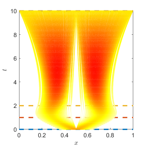
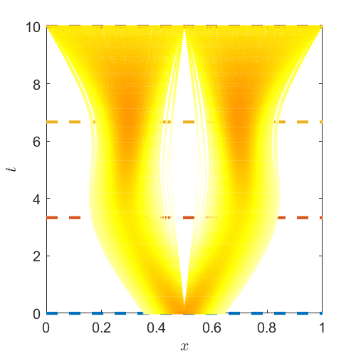
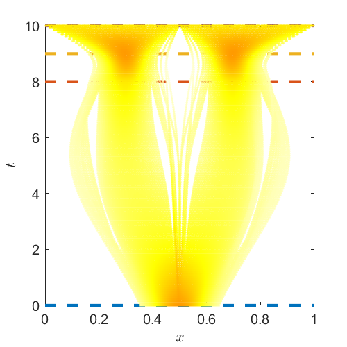
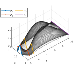
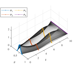
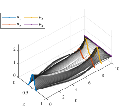
Figure 1: De Casteljau cone interpolation of measures $\mu_{1},\dots,\mu_{4}$. Measure values are shown as a heat map (top) and in a three-dimensional plot (bottom) as a function of time. Knot times $(t_{1},\dots,t_{4})$ are $(0,1,2,10)$ (left), $(0,\tfrac{10}{3},\tfrac{20}{3},10)$ (center), and $(0,8,9,10)$ (right). $\sigma=0.06$.

In this subsection, we look at the effects of time distribution of knots for a one dimensional cone spline problem. The map obtained from solving (7) is induced by a map only when the measures are absolutely continuous with respect to the Lebesgue measure. Indeed, the WFR plan from a single particle to two particles cannot be induced by a map. The same effect is present when solving problem (7) computationally. Here we choose to solve problem (7) using entropic regularization (Chizat et al.,, 2018; Peyré et al.,, 2019) and derive an approximation of the map from its solution by taking expectation of the marginals: $T(x)=\mathbb{E}_{\eta}[y|x]$, inspired by Pooladian and Niles-Weed, (2021).

Let $\gamma_{\sigma}(x)=\exp(-\tfrac{1}{2\sigma^{2}}x^{2})\mathds{1}_{[-2,2]}(x/\sigma).$ For our first experiment, we interpolate the measures

$$d\mu_{1}(x)=\gamma_{\sigma}\left(x-\tfrac{1}{2}\right)\,dx,$$

$$d\mu_{2}(x)=\tfrac{1}{2}\left(\gamma_{\sigma}(x-0.3)+\gamma_{\sigma}(x-0.7)\right)\,dx,$$

$$d\mu_{3}(x)=\left(\gamma_{\sigma}(x-0.3)+\gamma_{\sigma}(x-0.7)\right)\,dx,$$

$$d\mu_{4}(x)=\tfrac{1}{2}\mathds{1}_{[0,1]}(x)\,dx,$$

which we interpolate at three set of knot times $(t_{1},\dots,t_{4})$: $(0,1,2,10)$, $(0,\tfrac{10}{3},\tfrac{20}{3},10)$, and $(0,8,9,10)$ in figure 1.

5.2 Space discretization

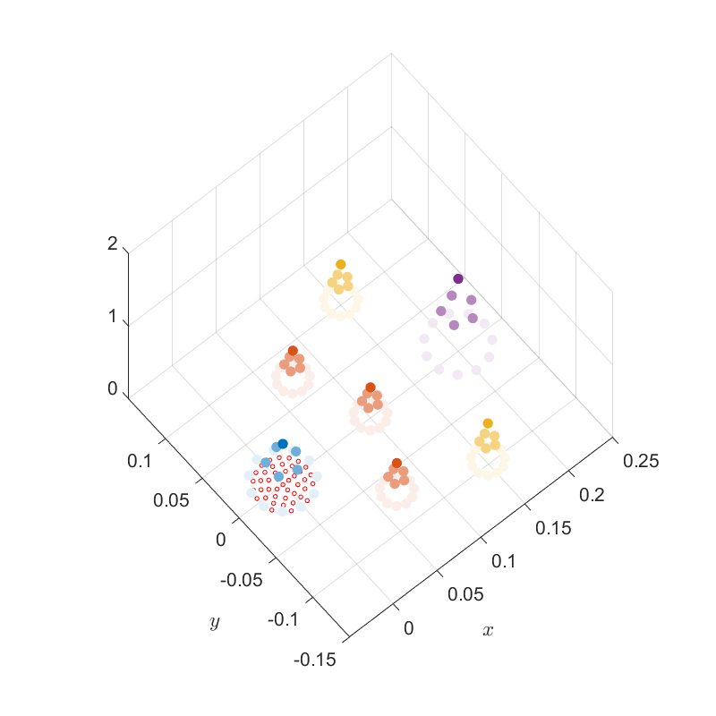
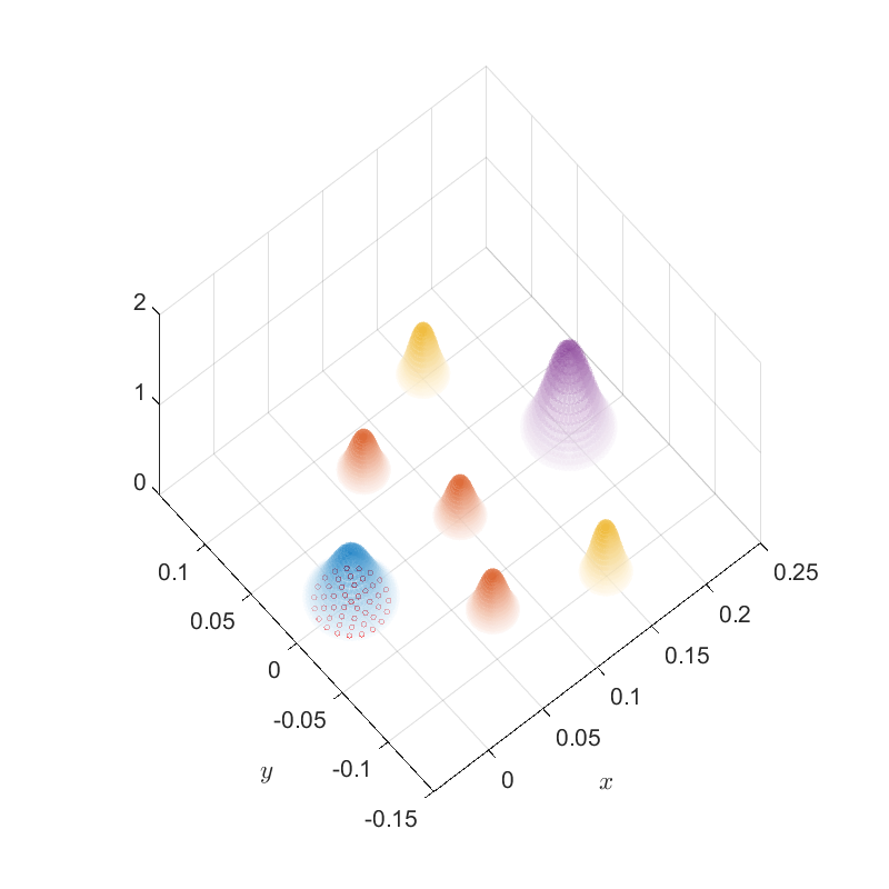
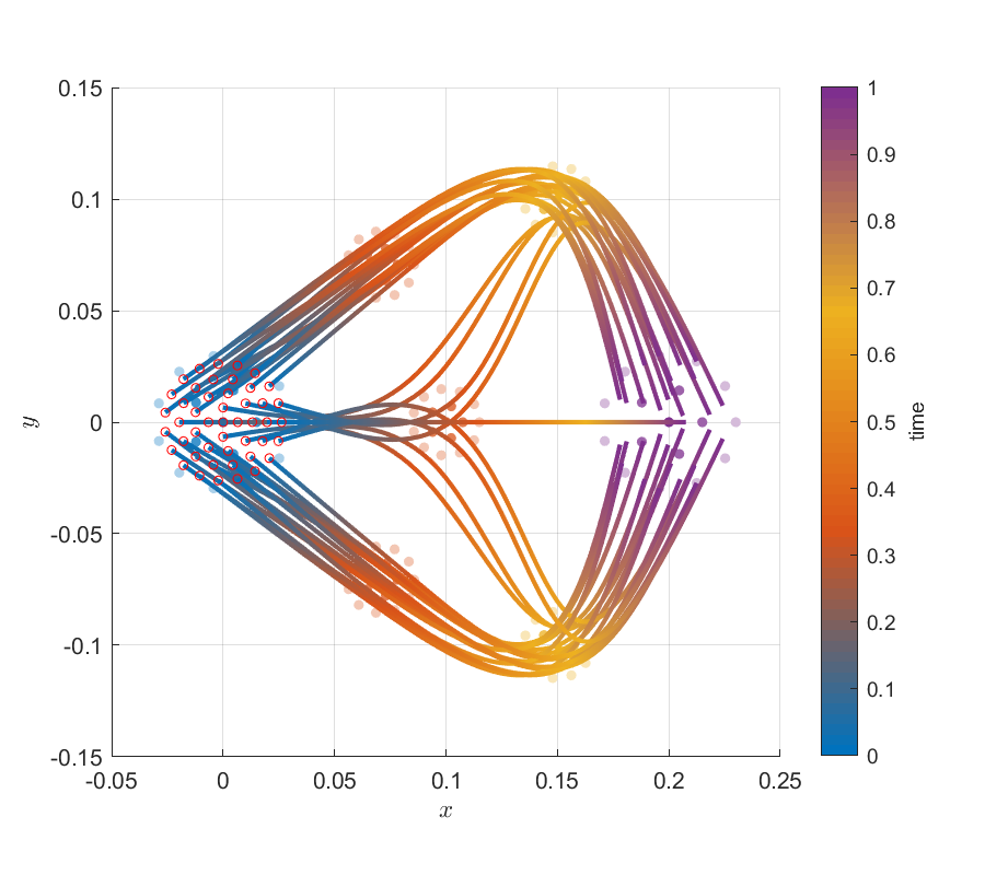
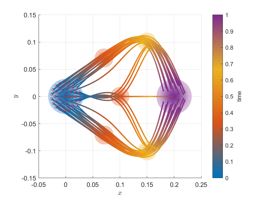
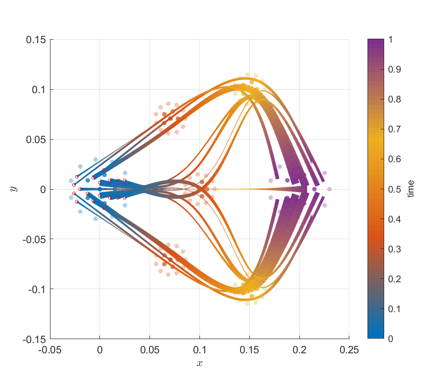
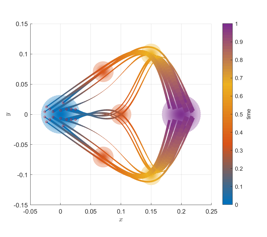
Figure 2: Subsampled (left) and gridded (right) interpolating measures. Measures $\mu_{1},\dots,\mu_{4}$ are shown in blue, orange, yellow, and purple respectively (top). Interpolated paths are computed for the points shown in red (middle) as a function of time varying by color. The width of select curves is changed according to the value of the measure (bottom). $\sigma=0.01$

We give details for the interpolation of measures in two dimensions in figure 2. For this example suppose we want to interpolate a set of particles. Since we need to represent them as absolutely continuous measures to be able to obtain a map, we convolve with a kernel and discretize the domain like in the previous section. As noted by Lavenant et al., (2021), gridding grows exponentially with the dimension which makes it infeasible for high-dimensional applications. We show here the result of fine gridding and compare it to sampling uniformly from the support.

Suppose the resulting interpolating measures are as follows. Let

$$\gamma_{\sigma}(x)=\exp(-\tfrac{1}{2\sigma^{2}}\|x\|^{2})\mathds{1}_{B_{2}(0)}(x).$$

We interpolate

$$d\mu_{1}(x)=\tfrac{3}{4}\gamma_{2\sigma}(x)\,dx,$$

$$d\mu_{2}(x)=0.65\left(\gamma_{\sigma}(x-(\tfrac{\sqrt{2}}{20},\tfrac{\sqrt{2}}{20}))+\gamma_{\sigma}(x-(0,-\tfrac{\sqrt{2}}{20}))+\gamma_{\sigma}(x-(\tfrac{\sqrt{2}}{20},-\tfrac{\sqrt{2}}{20}))\right)\,dx,$$

$$d\mu_{2}(x)=\tfrac{3}{4}\left(\gamma_{\sigma}(x-(\tfrac{3}{20},\tfrac{3}{20}))+\gamma_{\sigma}(x-(\tfrac{3}{20},-\tfrac{3}{20}))\right)\,dx,$$

$$d\mu_{4}(x)=\gamma_{2\sigma}(x-(\tfrac{1}{5},0))\,dx.$$

Appendix A Derivation of the covariant derivative

See 2

Proof.

Let $\mathbf{u}_{t}^{i}=(u_{t}^{i},\beta_{t}^{i})$ be two tangent fields along a curve $\mu_{t}$, which has derivative $(v_{t},\alpha_{t})$. Metric compatibility then reads

$$\frac{d}{dt}\langle\mathbf{u}_{t}^{1},\mathbf{u}_{t}^{2}\rangle_{\mu_{t}} =\int\langle\partial_{t}u_{t}^{1},u_{t}^{2}\rangle+\langle u_{t}^{1},\partial_{t}u_{t}^{2}\rangle+4\partial_{t}\beta_{t}^{1}\,\beta_{t}^{2}+4\beta_{t}^{1}\,\partial\beta_{t}^{2}\,d\mu_{t}$$

$$\quad+\int\langle u_{t}^{1},u_{t}^{2}\rangle+4\beta_{t}^{1}\beta_{t}^{2}\,d(\partial_{t}\mu_{t})$$

$$=T_{1}+T_{2}$$

By the continuity equation and the dual definition of $\operatorname{div}v_{t}\mu_{t}$, the second integral becomes

$$T_{2} =\int\langle\nabla u_{t}^{1}\cdot v_{t},u_{t}^{2}\rangle+\langle u_{t}^{2},\nabla u_{t}^{2}\cdot v_{t}\rangle+4\alpha_{t}\langle u_{t}^{1},u_{t}^{2}\rangle$$

$$\quad+\int 4\beta_{t}^{2}\langle\nabla\beta_{t}^{1},v_{t}\rangle+4\beta_{t}^{1}\langle\nabla\beta_{t}^{2},v_{t}\rangle+16\alpha_{t}\beta_{t}^{1}\beta_{t}^{2}\,d\mu_{t}$$

Now, we need this to be equal to $\langle\mathbf{u}_{t}^{1},\frac{\mathbf{D}}{dt}\mathbf{u}_{t}^{2}\rangle+\langle\frac{\mathbf{D}}{dt}\mathbf{u}_{t}^{1},\mathbf{u}_{t}^{2}\rangle$. Some terms are uniquely attributable to one or the other, such as $\int\langle\partial_{t}u_{t}^{1},u_{t}^{2}\rangle$, but some are not, such as $4\beta_{t}^{2}\langle\nabla\beta_{t}^{1},v_{t}\rangle$. This can arise from either of the two terms: as $\nabla\beta_{t}^{i}=u_{t}^{i}$,

$$\left\langle(0,\langle\nabla\beta_{t}^{1},v_{t}\rangle),\mathbf{u}_{t}^{2}\right\rangle_{\mu_{t}}=\left\langle\mathbf{u}_{t}^{1},(4\beta_{t}^{2}v,0)\right\rangle_{\mu_{t}}$$

Indeed, by splitting these terms and gathering the others, the possible covariant derivatives that satisfy metric compatibility are of the form

$$\frac{\mathbf{D}}{dt}\mathbf{u}_{t}=\mathcal{P}_{\mu_{t}}\begin{pmatrix}\partial_{t}u_{t}+\nabla u_{t}\cdot v_{t}+2\alpha_{t}u_{t}+4p\beta_{t}v_{t}\\ \partial_{t}\beta_{t}+(1-p)\langle\nabla\beta_{t},v_{t}\rangle+2\alpha_{t}\beta_{t}\end{pmatrix}$$

for real $p$. Let us check the torsion-free identity with $p=1/2$. In this case, if $\mathbf{u}_{t}=(\nabla\varphi,\varphi)$ is constant in time, then

$$\frac{\mathbf{D}}{dt}\begin{pmatrix}\nabla\varphi\\ \varphi\end{pmatrix}=\mathcal{P}_{\mu_{t}}\begin{pmatrix}\nabla^{2}\varphi\cdot v_{t}+2\alpha_{t}\nabla\varphi+2\varphi v_{t}\\ \frac{1}{2}\langle\nabla\varphi,v_{t}\rangle+2\alpha_{t}\varphi\end{pmatrix}$$

Now, with the setup as in the $W_{2}$ case, defining $F\colon\varphi\mapsto\int\varphi\,d\mu$ and writing $\bm{\varphi}=(\nabla\varphi,\varphi)$, we have from the continuity equation

$$\partial_{t}F[\mu_{t}^{i}]=\int\langle\bm{\varphi},\mathbf{v}_{t}^{i}\rangle\,d\mu_{t}^{i}$$

where $\mathbf{v}_{t}^{i}$ is the derivative of $\mu_{t}^{i}$. As above, we have

$$\mathbf{u}_{0}^{1}(\mathbf{u}^{2}(F))[\mu] =\frac{d}{dt}\langle\bm{\varphi},\mathbf{u}_{t}^{2}\rangle_{\mu_{t}^{2}}\big{|}_{t=0}$$

$$=\left\langle\frac{\mathbf{D}}{dt}\bm{\varphi},\mathbf{u}_{t}^{2}\right\rangle_{\mu_{t}^{2}}+\left\langle\bm{\varphi},\nabla_{\mathbf{u}_{0}^{1}}\mathbf{u}_{t}^{2}\right\rangle_{\mu_{t}^{2}}\bigg{|}_{t=0}$$

Recalling that at $t=0$ we have $\mathbf{u}_{0}^{2}=\mathbf{v}_{0}^{1}=(v_{0}^{1},\alpha_{0}^{1})$, the first term becomes (we may ignore the projection, since $\mathbf{u}_{t}^{2}$ is already tangent)

$$Q_{1}=\left\langle\begin{pmatrix}\nabla^{2}\varphi\cdot v_{0}^{2}+2\alpha_{0}^{2}\nabla\varphi+2\varphi v_{0}^{2}\\ \frac{1}{2}\langle\nabla\varphi,v_{0}^{2}\rangle+2\alpha_{0}^{2}\varphi\end{pmatrix},\begin{pmatrix}v_{0}^{1}\\ \alpha_{0}^{1}\end{pmatrix}\right\rangle_{\mu}$$

while the corresponding term from $\mathbf{u}_{0}^{2}(\mathbf{u}^{2}(F))[\mu]$ is

$$Q_{2}=\left\langle\begin{pmatrix}\nabla^{2}\varphi\cdot v_{0}^{1}+2\alpha_{0}^{1}\nabla\varphi+2\varphi v_{0}^{1}\\ \frac{1}{2}\langle\nabla\varphi,v_{0}^{1}\rangle+2\alpha_{0}^{1}\varphi\end{pmatrix},\begin{pmatrix}v_{0}^{2}\\ \alpha_{0}^{2}\end{pmatrix}\right\rangle_{\mu}$$

and we must check that these agree. The “top-left”, “top-right”, and “bottom-right” terms are identical for both. The top-middle of the first is equal to the bottom-left for the second, and vice-versa. Thus we have shown that the covariant derivative is given by

$$\frac{\mathbf{D}}{dt}\mathbf{u}_{t}=\mathcal{P}_{\mu_{t}}\begin{pmatrix}\partial_{t}u_{t}+\nabla u_{t}\cdot v_{t}+2\alpha_{t}u_{t}+2\beta_{t}v_{t}\\ \partial_{t}\beta_{t}+\frac{1}{2}\langle\nabla\beta_{t},v_{t}\rangle+2\alpha_{t}\beta_{t}\end{pmatrix}$$

and in specific,

$$\frac{\mathbf{D}^{2}}{dt^{2}}\mu_{t}=\begin{pmatrix}\partial_{t}v_{t}+\nabla v_{t}\cdot v_{t}+4\alpha_{t}v_{t}\\ \partial_{t}\alpha_{t}+\frac{1}{2}|\nabla\alpha_{t}|^{2}+2\alpha_{t}^{2}\end{pmatrix}$$ (20)

This quantity is tangent, so no projection is necessary. ∎

Appendix B Proof of equivalence in curvature

See 6

Proof.

Making the definition explicit, we wish of our measure $P$ that the cost of (12) is equal to

$$\int_{0}^{1}\int\left|\partial_{t}v_{t}+\nabla v_{t}\cdot v_{t}+4\alpha_{t}v_{t}\right|^{2}+4\left(\partial_{t}\alpha_{t}+\tfrac{1}{2}|\nabla\alpha_{t}|^{2}+2\alpha_{t}^{2}\right)^{2}\,d\mu_{t}\,dt$$ (21)

Let $\lambda_{0}\in\mathcal{P}(\mathfrak{C})$ be a lift of $\mu_{0}$. By Proposition 2, the measure $\lambda_{t}=(X_{t},R_{t})_{\#}\lambda_{0}$ is a lift of $\mu_{t}$.

In order to compute the covariant derivative of a curve on the cone, we compute the Christoffel symbols. These are given by the formulas

$$\nabla_{\partial x_{i}}\partial x_{j}=\Gamma_{ij}^{k}\partial_{k},\quad\Gamma_{ij}^{k}=\frac{1}{2}g^{kl}\left(\frac{\partial}{\partial_{j}}g_{il}+\frac{\partial}{\partial_{i}}g_{jl}-\frac{\partial}{\partial_{l}}g_{ij}\right).$$

Let $\partial x_{1},\dots,\partial x_{n},\partial_{r}$ be the coordinate basis of the tangent space on the cone, hence

$$(g_{ij})_{ij}=\begin{pmatrix}r^{2}I_{n}&0\\ 0&1\end{pmatrix},\quad\frac{\partial}{\partial_{k}}g_{ij}=\begin{cases}2r&i=j\neq r,~{}k=r,\\ 0,&\text{else}.\end{cases}$$

Since $(g^{ij})$ and $\partial_{r}g_{ij}$ are only defined along the diagonal and $\partial_{l}g_{ij}=0$ for $l\neq r$, the only terms that do not vanish are

$$\Gamma_{rj}^{k}=r^{-1}\delta_{jk},\quad\Gamma_{ij}^{r}=-r\delta_{ij}$$

thus the Levi-Civita connection on the cone is given by

$$\nabla_{\partial_{r}}\partial_{r}=0,\quad\quad\nabla_{\partial_{r}}X=r^{-1}X,\quad\quad\nabla_{X_{1}}X_{2}=-r\langle X_{1},X_{2}\rangle\partial_{r}.$$

From this, the covariant derivative of a curve $z_{t}=(x_{t},r_{t})$ on the cone is given by

$$\ddot{z}_{t}=\nabla_{\dot{z}_{t}}\dot{z}_{t}=\left(\ddot{x}_{t}+2\frac{\dot{r}_{t}}{r_{t}}\dot{x}_{t},~{}\ddot{r}_{t}-r_{t}|\dot{x}_{t}|^{2}\right)$$

thus from the Riemannian metric (11)

$$|\ddot{z}_{t}|^{2}=\left|r_{t}\ddot{x}_{t}+2\dot{r}_{t}\dot{x}_{t}\right|^{2}+\left|\ddot{r}_{t}-r_{t}|\dot{x}_{t}|^{2}\right|^{2}$$

Let $\lambda_{0}$ be any lift of $\mu_{0}$ and define $P$ to place mass $\lambda_{0}(z_{0})$ on the path $z_{t}=(X_{t}(x_{0}),R_{t}(r_{0}))$, so that $P$ is supported on the flow map curves in $\Omega_{\mathfrak{C}}$. By applying the total derivative to the defining equations of the flow maps, these curves satisfy

$$\dot{x}_{t} =v_{t}(x_{t})$$

$$\ddot{x}_{t} =\partial_{t}v_{t}+\nabla v_{t}\cdot v_{t}$$

$$\dot{r}_{t} =2r_{t}\alpha_{t}(x_{t})$$

$$\ddot{r}_{t} =2r_{t}\left(\partial_{t}\alpha_{t}+\nabla\alpha_{t}\cdot v_{t}+2\alpha_{t}^{2}\right)$$

Now, we have

$$\int_{\Omega_{\mathfrak{C}}}\int_{0}^{1}|\ddot{z}_{t}|^{2}\,dt\,dP(z)=\int_{\mathfrak{C}}\int_{0}^{1}|\ddot{z}_{t}|^{2}\,dt\,d\lambda_{0}(z_{0})$$

Expanding out, this is

$$\int_{\mathfrak{C}}\int_{0}^{1}\left|r_{t}\ddot{x}_{t}+2\dot{r}_{t}\dot{x}_{t}\right|^{2}+\left|\ddot{r}_{t}-r_{t}|\dot{x}_{t}|^{2}\right|^{2}\,dt\,d\lambda_{0}(z_{0})$$

Let us deal with each term separately so the expressions do not become unwieldly. For the first

$$\int_{\mathfrak{C}}\int_{0}^{1}\left|r_{t}\ddot{x}_{t}+2\dot{r}_{t}\dot{x}_{t}\right|^{2}\,dt\,d\lambda_{0}(z_{0})$$

$$= \int_{\mathfrak{C}}\int_{0}^{1}r_{t}^{2}\left|\partial_{t}v_{t}+\nabla v_{t}\cdot v_{t}+4\alpha_{t}v_{t}\right|^{2}(x_{t})\,dt\,d\lambda_{0}(z_{0})$$

$$= \int_{0}^{1}\int_{\mathfrak{C}}\left|\partial_{t}v_{t}+\nabla v_{t}\cdot v_{t}+4\alpha_{t}v_{t}\right|^{2}(x_{t})\,d(r_{t}^{2}\cdot\lambda_{0})(z_{0})\,dt$$

$$= \int_{0}^{1}\int\left|\partial_{t}v_{t}+\nabla v_{t}\cdot v_{t}+4\alpha_{t}v_{t}\right|^{2}(x)\,d\mu_{t}(x)\,dt$$

We have used that $(X_{t},R_{t})_{\#}\lambda_{0}=\lambda_{t}$ and $\mathfrak{P}\lambda_{t}=\mu_{t}$. The second term is dealt with in exactly the same way,

$$\int_{\mathfrak{C}}\int_{0}^{1}\left|\ddot{r}_{t}-r_{t}|\dot{x}_{t}|^{2}\right|^{2}\,dt\,d\lambda_{0}(z_{0})$$

$$= \int_{\mathfrak{C}}\int_{0}^{1}4r_{t}^{2}\left|\partial_{t}\alpha_{t}+\tfrac{1}{2}\nabla\alpha_{t}\cdot v_{t}+2\alpha_{t}^{2}\right|^{2}(x_{t})\,dt\,d\lambda_{0}(z_{0})$$

$$= \int_{0}^{1}\int_{\mathfrak{C}}4\left|\partial_{t}\alpha_{t}+\tfrac{1}{2}\nabla\alpha_{t}\cdot v_{t}+2\alpha_{t}^{2}\right|^{2}(x_{t})\,d(r_{t}^{2}\cdot\lambda_{0})(z_{0})\,dt$$

$$= \int_{0}^{1}\int_{\mathfrak{C}}4\left|\partial_{t}\alpha_{t}+\tfrac{1}{2}\nabla\alpha_{t}\cdot v_{t}+2\alpha_{t}^{2}\right|^{2}(x_{t})\,d\mu_{t}(x)\,dt.$$

∎

Appendix C Cone De Casteljau’s algorithm

See 3

Proof.

Let $\theta_{i}:=|x_{i+1}-x_{i}|$. Since the expressions for $w$, $u$ and $P$ are all the same with different interpolating points, we compute the derivatives of $w$ $\rho$, $r$ and $\theta$ with the suscripts removed. To compute each derivative, we just replace with the corresponding suscript.

For $\theta=|x_{1}-x_{0}|$,

$$\theta\dot{\theta} =\langle x_{1}-x_{0},\dot{x}_{1}-\dot{x}_{0}\rangle.$$

For a point $w_{0}=(1-\rho)x_{0}+\rho x_{1}$,

$$\dot{w}_{0} =(x_{1}-x_{0})\dot{\rho}+(1-\rho)\dot{x}_{0}+\rho\dot{x}_{1}.$$ (22)

For the mass $r^{2}=r_{0}^{2}(1-t)^{2}+r_{1}^{2}t^{2}+2r_{0}r_{1}t(1-t)\cos(\theta)$,

$$r\dot{r}=~{} 2r_{0}\dot{r}_{0}(1-t)^{2}-r_{0}^{2}(1-t)+r_{1}\dot{r}_{1}t^{2}+r_{1}^{2}t$$ (23)

$$+(\dot{r}_{1}r_{0}+\dot{r}_{0}r_{1})t(1-t)\cos(\theta)$$

$$+r_{0}r_{1}(1-2t)\cos(\theta)-r_{0}r_{1}t(1-t)\sin(\theta)\dot{\theta}.$$

For the local time $\rho=\frac{1}{\theta}\arccos\left(\frac{r_{0}(1-t)+r_{1}t\cos(\theta)}{r}\right)$,

$$\dot{\rho}\theta+\rho\dot{\theta}=~{} \frac{1}{r_{w_{0}}^{2}}\big{(}(1-t)t\sin(\theta)(\dot{r}_{1}r_{0}-\dot{r}_{0}r_{1})$$ (24)

$$+(1-t)t\cos(\theta)r_{0}r_{1}\dot{\theta}$$

$$+r_{0}r_{1}\sin(\theta)+r_{1}^{2}\dot{\theta}t^{2}\big{)}.$$

For the first interpolation points $w_{0},w_{1},w_{2}$ we have in particular that $\dot{x}_{i},\dot{r}_{x_{i}}=0$, hence

$$\dot{\theta}_{w_{i}} =0,$$

$$\dot{w}_{i} =(x_{i+1}-x_{i})\dot{\rho}_{w_{i}},$$

$$\dot{r}_{w_{i}} =\frac{1}{r_{w_{i}}}\left(-r_{x_{i}}^{2}(1-t)+r_{x_{i+1}}^{2}t+r_{x_{i}}r_{x_{i+1}}(1-2t)\cos(\theta_{w_{i}})\right),$$

$$\dot{\rho}_{w_{i}} =\frac{r_{x_{i}}r_{x_{i+1}}}{\theta_{w_{i}}}\sin(\theta_{w_{i}})-\rho_{w_{i}}\frac{\dot{\theta}_{w_{i}}}{\theta_{w_{i}}}.$$

Thus at $t=0$,

$$\dot{\theta}_{w_{i}}(0) =0$$ (25)

$$\dot{\rho}_{w_{i}}(0) =\frac{r_{x_{i+1}}}{r_{x_{i}}}\frac{\sin(\theta_{i})}{\theta_{i}}$$ (26)

$$\dot{r}_{w_{i}}(0) =r_{x_{i+1}}\cos(\theta_{i})-r_{x_{i}}$$ (27)

$$\dot{w}_{i}(0) =(x_{i+1}-x_{i})\frac{r_{x_{i+1}}}{r_{x_{i}}}\frac{\sin(\theta_{i})}{\theta_{i}}$$ (28)

and $t=1$,

$$\dot{\theta}_{w_{i}}(1) =0$$ (29)

$$\dot{\rho}_{w_{i}}(1) =\frac{r_{x_{i}}}{r_{x_{i+1}}}\frac{\sin(\theta_{i})}{\theta_{i}}$$ (30)

$$\dot{r}_{w_{i}}(1) =r_{x_{i+1}}-r_{x_{i}}\cos(\theta_{i})$$ (31)

$$\dot{w}_{i}(1) =(x_{i+1}-x_{i})\frac{r_{x_{i}}}{r_{x_{i+1}}}\frac{\sin(\theta_{i})}{\theta_{i}}.$$ (32)

We substitute these expression back into the formulas for the derivatives of position (22), mass (23) and local time (24) for $u_{j}$ and $p$, for $j=0,1$. Notice that for both $t=0$ and $t=1$ the depdence on $\dot{\theta}$ vanishes.

$$\dot{\rho}_{u_{j}}(0) =\frac{r_{x_{j+1}}}{r_{x_{j}}}\frac{\sin(\theta_{j})}{\theta_{j}}$$ (33)

$$\dot{r}_{u_{j}}(0) =2\left(r_{x_{j+1}}\cos(\theta_{j})-r_{j}\right)$$ (34)

$$\dot{u}_{j}(0) =2(x_{j+1}-x_{j})\frac{r_{x_{j+1}}}{r_{x_{j}}}\frac{\sin(\theta_{j})}{\theta_{j}}$$ (35)

$$\dot{\rho}_{u_{j}}(1) =\frac{r_{x_{j}}}{r_{x_{j+1}}}\frac{\sin(\theta_{{j+1}})}{\theta_{j+1}}$$ (36)

$$\dot{r}_{u_{j}}(1) =2\left(r_{x_{j+1}}-r_{x_{j}}\cos(\theta_{j+1})\right)$$ (37)

$$\dot{u}_{j}(1) =2(x_{j+1}-x_{j})\frac{r_{x_{j+1}}}{r_{x_{j}}}\frac{\sin(\theta_{j+1})}{\theta_{j+1}}$$ (38)

Finally for $p$,

$$\dot{\rho}_{p}(0) =\frac{r_{x_{1}}}{r_{x_{0}}}\frac{\sin(\theta_{0})}{\theta_{0}},$$ (39)

$$\dot{r}_{p}(0) =3\left(r_{x_{1}}\cos(\theta_{0})-r_{x_{0}}\right),$$ (40)

$$\dot{p}(0) =3(x_{1}-x_{0})\frac{r_{x_{1}}}{r_{x_{0}}}\frac{\sin(\theta_{0})}{\theta_{0}},$$ (41)

$$\dot{\rho}_{p}(1) =\frac{r_{x_{2}}}{r_{x_{3}}}\frac{\sin(\theta_{2})}{\theta_{2}},$$ (42)

$$\dot{r}_{p}(1) =3\left(r_{x_{3}}-r_{x_{2}}\cos(\theta_{2})\right),$$ (43)

$$\dot{p}(1) =3(x_{3}-x_{2})\frac{r_{x_{2}}}{r_{x_{3}}}\frac{\sin(\theta_{2})}{\theta_{2}}.$$ (44)

∎

References

• Absil et al., (2016) Absil, P.-A., Gousenbourger, P.-Y., Striewski, P., and Wirth, B. (2016). Differentiable piecewise-bézier surfaces on riemannian manifolds. SIAM Journal on Imaging Sciences, 9(4):1788–1828.