Scale-mixture Birnbaum-Saunders quantile regression models applied to personal accident insurance data

Abstract. The modeling of personal accident insurance data has been a topic of extreme relevance in the insurance literature. This kind of data often exhibits positive skewness and heavy tails. In this work, we propose a new quantile regression model based on the scale-mixture Birnbaum-Saunders distribution for modeling personal accident insurance data. The maximum likelihood estimates of the model parameters are obtained via the EM algorithm. Two Monte Carlo simulation studies are performed using the R software. The first study aims to analyze the performances of the EM algorithm to obtain the maximum likelihood estimates, and the randomized quantile and generalized Cox-Snell residuals. In the second simulation study, the size and power of the the Wald, likelihood ratio, score and gradient tests are evaluated. The two simulation studies are conducted considering different quantiles of interest and sample sizes. Finally, a real insurance data set is analyzed to illustrate the proposed approach.

Keywords: Scale-mixture Birnbaum-Saunders distribution; EM algorithm; Hypothesis tests; Monte Carlo simulation; Quantile regression.

1 Introduction

Birnbaum-Saunders (BS) regression models have proven to be good alternatives in insurance data modeling; see Leiva, (2016) and Naderi et al., (2020). Usually, this kind of data shows positive skewness and heavy tails. Paula et al., (2012), for example, used the BS-Student-$t$-BS regression model to study how some explanatory variables (covariates) influence the amount of paid money by an insurance policy. The Student-$t$-BS distribution is a special case of the class of scale-mixture Birnbaum-Saunders (SBS) distributions, which was proposed by Balakrishnan et al., (2009) and is based on the relationship between the class of scale mixtures of normal (SMN) and BS distributions. The main advantage of the SBS distributions over the classical BS distribution (Leiva,, 2016; Balakrishnan and Kundu,, 2019) is their capability to make robust estimation of parameters in a way similar to that of SMN models, in addition to facilitating the implementation of an expectation maximization (EM) algorithm; see Balakrishnan et al., (2009). Recently, Lachos et al., (2017) proposed a Bayesian regression model based on the SBS distributions for censored data.

The class of SMN distributions comprises a family of symmetric distributions studied initially by Andrews and Mallows, (1974). These distributions have been gaining considerable attention with the publication of some works, as can be seen in Efron and Olshen, (1978), West, (1987), Lange and Sinsheimer, (1993), Gneiting, (1997), Taylor and Verbyla, (2004), Walker and Gutiérrez-Peña, (2007) and Lachos and Labra, (2007). This family of distributions has as special cases flexible distributions with heavy-tails, which are often employed for robust estimation; see Lange et al., (1989) and Lucas, (1997).

Quantile regression models emerged as a broader proposal in the analysis of the relationship between the response variable and the respective covariates of a regression model. These models were initially studied by Koenker and Bassett Jr, (1978) and have since been increasingly used in regression analysis; see Koenker and Hallock, (2001), Yu and Moyeed, (2001) and Koenker, (2004). Quantile regression models are robust alternatives in relation to the regression models for mean because the process of estimating parameters of the quantile regression model is not subject to the influence of outliers as in the case of linear regression. Moreover, these models are capable of showing different effects of covariates on the response along the quantiles of response variable.

In this work, we propose a new parametric quantile regression model for strictly positive data based on a reparameterization of the SBS distributions. We first introduce a reparameterization of the SBS model by inserting a quantile parameter, and then develop the new SBS quantile regression model. In addition to the quantile approach, another advantage in relation to the regression approach developed in Lachos et al., (2017) is the modeling of dependent variable without the need of applying the logarithm transformation, which can cause problems with regard to interpretation and loss in power of the study; see Huang and Qu, (2006) for an explanation. We illustrate the proposed methodology by using the insurance data set studied by Paula et al., (2012). The results show that a quantile approach provides a richer characterization of the effects of covariates on the dependent variable.

The rest of this paper is organized as follows. In Section 2, we describe the usual SBS distribution and propose a reparameterization of this distribution in terms of a quantile parameter. In this section, we also discuss some mathematical properties of the proposed reparameterized model. In Section 3, we introduce the SBS quantile regression model. In this section, we also describe the steps o the EM algorithm (Dempster et al.,, 1977) for maximum likelihood (ML) estimation of the model parameters, the standard error calculation, hypothesis tests, model selection criteria and residuals. In Section 4, we carry out two Monte Carlo simulation studies. In the first simulation study, we evaluate the performance of the EM algorithm through the calculated biases, mean square errors (MSEs) and coverage probabilities of the asymptotic confidence intervals. We also evaluate the performances of residuals, such as the generalized Cox-Snell –GCS– (Cox and Snell,, 1968) and randomized quantile –RQ– residuals (Dunn and Smyth,, 1996), for assessing the goodness-of-fit and identifying any departure from model assumptions. In the second simulation study, we assess the performances of formal test procedures such as the likelihood ratio test, score test, Wald test and gradient test. In Section 5, we apply the SBS quantile regression model to a real insurance data set. Finally, in Section 6, we make some concluding remarks and discuss potential future research problems.

2 Preliminaries

In this section, we first present the SBS distribution. Then, we present the proposed quantile-based SBS distribution, which we call as QSBS distribution. Some properties and special cases of the QSBS distribution are also discussed.

2.1 SBS distribution

Let $Y$ be a random variable (RV) whose stochastic representation can be written as follows:

$$Y=\mu+\sqrt{g(U)}X,$$ (1)

where $\mu$ is a location parameter, $X\sim\text{N}(0,\sigma^{2})$ with $\sigma>0$, $U$ is a RV distributed independent of $X$ and having cumulative distribution function (CDF) $H(\cdot)$, which is indexed by an extra parameter ${\nu}$ (or extra parameter vector $\bm{\nu}$), and $g(\cdot)$ is a strictly positive function. Note that when $g(U)=1/U$, the distribution of $Y$ in (1) reduces to the normal/independent distribution, presented in Lange and Sinsheimer, (1993). Similarly, when $g(U)=U$ in (1), the distribution of $Y$ reduces to the SMN distribution, studied by Fernández and Steel, (1999).

The probability density function (PDF) of $Y$, a RV that follows a SMN distribution with location and scale parameters $\mu\in\mathbb{R}$ and $\sigma^{2}>0$, respectively, is given by the following Lebesgue-Stieltjes integral:

$$\phi_{\text{SMN}}(y)=\int_{\color[rgb]{0,0,0}\definecolor[named]{pgfstrokecolor}{rgb}{0,0,0}\pgfsys@color@gray@stroke{0}\pgfsys@color@gray@fill{0}(0,\infty)\cap{\rm Supp}(U)}\phi(y;\mu,g(u)\sigma^{2})dH(u),{\color[rgb]{0,0,0}\definecolor[named]{pgfstrokecolor}{rgb}{0,0,0}\pgfsys@color@gray@stroke{0}\pgfsys@color@gray@fill{0}\quad y\in\mathbb{R},}$$ (2)

where ${\rm Supp}(U)$ is the support of $U$, $\phi({\color[rgb]{0,0,0}\definecolor[named]{pgfstrokecolor}{rgb}{0,0,0}\pgfsys@color@gray@stroke{0}\pgfsys@color@gray@fill{0}\cdot};\mu,g(u)\sigma^{2})$ is the normal PDF with mean $\mu$ and variance $g(u)\sigma^{2}$, and $H(u)$ is the CDF of $U$. Let us denote $Y\sim\text{SMN}(\mu,\sigma^{2};H)$. When $\mu=0$ and $\sigma^{2}=1$, we denote $Y\sim\text{SMN}(H)$.

According to Balakrishnan et al., (2009), a RV $T$ follows a SBS distribution if it has the following stochastic representation:

$$T=\frac{\beta}{4}\left[\alpha{\color[rgb]{0,0,0}\definecolor[named]{pgfstrokecolor}{rgb}{0,0,0}\pgfsys@color@gray@stroke{0}\pgfsys@color@gray@fill{0}Y}+\sqrt{(\alpha{\color[rgb]{0,0,0}\definecolor[named]{pgfstrokecolor}{rgb}{0,0,0}\pgfsys@color@gray@stroke{0}\pgfsys@color@gray@fill{0}Y})^{2}+4}\right]^{2},$$ (3)

where $Y=\sqrt{g(U)}Z\sim\text{SMN}(H)$, such that $Z\sim\text{N}(0,1)$ and $\alpha>0$ and $\beta>0$ are the shape and scale parameters, respectively, of the BS distribution. In this case, the notation $T\sim\text{SBS}(\alpha,\beta;H)$ is used. When $Y\sim\text{N}(0,1)$, then $T$ follows a classical BS distribution. The PDF of $T\sim\text{SBS}(\alpha,\beta;H)$ can be expressed as

$$f_{T}(t)=\phi_{\text{SMN}}(a(t))a^{\prime}(t),\quad t>0,$$ (4)

where $\phi_{\text{SMN}}(\cdot)$ is the PDF given in (2) with $\mu=0$ and $\sigma^{2}=1$, $a(t)=\bigl{(}\sqrt{t/\beta}-\sqrt{\beta/t}\,\bigr{)}/\alpha$, and $a^{\prime}(t)=t^{-3/2}(t+\beta)/(2\alpha\beta^{1/2})$ is the derivative of $a(t)$ with respect to $t$. The CDF of $T$ is given by

$$F_{T}(t)=\Phi_{\text{SMN}}(a(t)),\quad t>0,$$ (5)

where $\Phi_{\text{SMN}}(\cdot)$ is the CDF of the $\text{SMN}(H)$ distribution. The $100q-$th quantile of $T\sim\text{SBS}(\alpha,\beta;H)$ is given by

$$Q=t_{q}=\frac{\beta}{4}\left[\alpha y_{q}+\sqrt{(\alpha y_{q})^{2}+4}\right]^{2},$$ (6)

where $y_{q}$ is the $q\times 100$-th quantile of $Y\sim\text{SMN}(H)$.

2.2 Quantile-based SBS distributions

Consider a fixed number $q\in(0,1)$ and the one-to-one transformation $(\alpha,\beta;H)\longmapsto(\alpha,Q;H),$ where $Q$ is the $100q$-th quantile of $T\sim\text{SBS}(\alpha,\beta;H)$ defined in (6). Then, we obtain the following stochastic representation based on a quantile parameter:

$$T=\frac{Q}{\gamma_{\alpha}^{2}}\left[\alpha\sqrt{g(U)}Z+\sqrt{\big{(}\alpha\sqrt{g(U)}Z\big{)}^{2}+4}\right]^{2},$$ (7)

where $\gamma_{\alpha}=\alpha y_{q}+\sqrt{(\alpha y_{q})^{2}+4}$, $Z\sim\text{N}(0,1)$, and $g(U)=1/U$ is such that the distribution of $g(U)$ has a known PDF. The stochastic representation (7) can be used to generate random numbers, to obtain the moments, and also in the implementation of the EM algorithm.

From the stochastic representation (7), we obtain a quantile-based reparameterization of the SBS distribution with CDF and PDF given, respectively, by

$$\begin{array}[]{lllll}\displaystyle F_{T}(t)=\Phi_{\text{SMN}}(a(t))\,{\color[rgb]{0,0,0}\definecolor[named]{pgfstrokecolor}{rgb}{0,0,0}\pgfsys@color@gray@stroke{0}\pgfsys@color@gray@fill{0}=\int_{(0,\infty)\cap{\rm Supp}(U)}\Phi\big{(}a_{\scaleto{\sqrt{g(u)}}{9pt}}(t)\big{)}dH(u)},\quad t>0,\\[17.07182pt] \displaystyle f_{T}(t)=\phi_{\text{SMN}}(a(t))a^{\prime}(t)\,{\color[rgb]{0,0,0}\definecolor[named]{pgfstrokecolor}{rgb}{0,0,0}\pgfsys@color@gray@stroke{0}\pgfsys@color@gray@fill{0}=\int_{(0,\infty)\cap{\rm Supp}(U)}\phi\big{(}a_{\scaleto{\sqrt{g(u)}}{9pt}}(t)\big{)}a^{\prime}_{\scaleto{\sqrt{g(u)}}{9pt}}(t)dH(u)},\quad t>0,\end{array}$$ (8)

where $\Phi(\cdot)$ and $\phi(\cdot)$ are the CDF and PDF of the standard normal distribution, respectively, $a_{x}(t)=\bigl{(}\sqrt{\gamma_{\alpha x}^{2}t/4Q}-\sqrt{4Q/\gamma_{\alpha x}^{2}t}\,\bigr{)}/{(\alpha x)}$, $a^{\prime}_{x}(t)=(\gamma_{\alpha x}^{2}/2+2Q/t)/(\alpha x\gamma_{\alpha x}\sqrt{4Qt})$ and $\gamma_{\alpha}=\alpha y_{q}+\sqrt{(\alpha y_{q})^{2}+4}$. In this case, the notation $T\sim\text{QSBS}(\alpha,Q;H)$ is used. Some properties of the QSBS distribution are presented below.

Proposition 1.

If $T\sim\text{QSBS}(\alpha,Q;H)$ then $\lim_{t\to 0^{+}}f_{T}(t)=\lim_{t\to\infty}f_{T}(t)=0.$

Proof.

Since $f_{T}(\cdot)$ is a PDF, it is clear that $\lim_{t\to\infty}f_{T}(t)=0$. On the other hand, by (8) we observe that $f_{T}(t)=\int_{(0,\infty)\cap{\rm Supp}(U)}f_{S_{u}}(t)dH(u)$, where $f_{S_{u}}(\cdot)$ is the corresponding PDF of a RV $S_{u}$ having a quantile-based Birnbaum-Saunders (QBS) distribution with parameters $\alpha\sqrt{u}$ and $Q$, denoted by $S_{u}\sim\text{QBS}\big{(}\alpha\sqrt{g(u)},Q\big{)}$. It is well-known that the QBS distribution is unimodal. Then there is a unique $t_{0}=t_{0}\big{(}\alpha\sqrt{g(u)},Q\big{)}>0$ such that $f_{S_{u}}(t)\leqslant\max\{{f_{S_{u}}(t)}:t>0\}=f_{S_{u}}(t_{0})\leqslant\max\{f_{S_{u}}(t_{0}):u>0\}$. Applying the bounded convergence theorem, we have $\lim_{t\to 0^{+}}f_{T}(t)=\int_{(0,\infty)\cap{\rm Supp}(U)}\lim_{t\to 0^{+}}f_{S_{u}}(t)dH(u)=0$ because $\lim_{t\to 0^{+}}f_{S_{u}}(t)=0$. This completes the proof. ∎

Proposition 2.

If $g(\cdot)$ in (1) is chosen such that the function

$$G(t)={\phi^{\prime}_{\text{SMN}}(a(t))\over\phi_{\text{SMN}}(a(t))}+{a^{\prime\prime}(t)\over[a^{\prime}(t)]^{2}},\quad t>0$$

has a unique zero $t=t_{0}$, then the QSBS PDF (8) is unimodal.

Proof.

Suppose that $g(\cdot)$ is such that $G(t_{0})=0$. A simple calculus shows that $f_{T}^{\prime}(t)=f_{T}(t)a^{\prime}(t)G(t)$. Then $f_{T}^{\prime}(t_{0})=0$ because $G(t_{0})=0$, $f_{T}(t)>0$ and $a^{\prime}(t)>0$. That is, $t_{0}$ is the unique critical point of $f_{T}(\cdot)$. Furthermore, by Proposition 1, $\lim_{t\to 0^{+}}f_{T}(t)=\lim_{t\to\infty}f_{T}(t)=0$. Consequently, the QSBS PDF is increasing on $(0,t_{0})$ and is decreasing on $(t_{0},\infty)$. This proves the unimodality. ∎

In the proofs of the following propositions, we adopt the following notations: $a_{x}(t)=a_{x}(t;\alpha,Q)$ and $a(t)=a(t;\alpha,Q)=a_{1}(t)$.

Proposition 3.

Let $T\sim\text{QSBS}(\alpha,Q;H)$. Then, $T$ allows the following conditional stochastic representation:

$$T|U=u\sim\text{QBS}\big{(}\alpha\sqrt{g(u)},Q\big{)}.$$

Proof.

If $U=u$ then $T=a^{-1}\big{(}\sqrt{g(u)}Z\big{)}$. Thus, the conditional distribution of $T$ given $U=u$ is the same as the distribution of the elements presented as $a^{-1}\big{(}\sqrt{g(u)}Z\big{)}|U=u.$ This implies that $F_{T}(t|U=u)=\Phi\big{(}a(t)/\sqrt{g(u)}\big{)}=\Phi\big{(}a_{\scaleto{\sqrt{g(u)}}{9pt}}(t)\big{)}$ because $U$ is independent of $Z$. Then, the proof follows. ∎

Let $T\sim\text{QSBS}(\alpha,Q;H)$ and $f$ be a Borel measurable function. Then, by using the law of total expectation, we have

$$\mathbb{E}[f(T)]=\mathbb{E}[\mathbb{E}[f(T)|U]]=\int_{(0,\infty)\cap{\rm Supp}(U)}\mathbb{E}[f(T)|U=u]dH(u).$$ (9)

By taking $f(t)=\exp(ist)$, $s\in\mathbb{R}$, in (9), where $i=\sqrt{-1}$ is the unit imaginary number, from Proposition 3 and Formula (2.13) of Leiva, (2016), we get the following result:

Proposition 4.

Let $T\sim\text{QSBS}(\alpha,Q;H)$. Then, the characteristic function of $T$, denoted by $\phi_{T}(s)=\mathbb{E}(\exp(isT))$, can be written as

$$\phi_{T}(s)={1\over 2}\,\mathbb{E}\left[\left(1+\frac{1}{\sqrt{1-2i({4Q}/{\gamma_{\alpha}^{2}})s^{2}g(U)}}\right)\exp\left(\frac{1-\sqrt{1-2i({4Q}/{\gamma_{\alpha}^{2}})s^{2}g(U)}}{\alpha^{2}g(U)}\right)\right].$$

Taking $k$ consecutive partial derivatives of $\phi_{T}(s)$ with respect to $s$, assuming that we can interchange the derivative with the expectation, and then evaluating at $s=0$ and dividing by $i^{k}$, we get the following result:

Proposition 5.

Let $T\sim\text{QSBS}(\alpha,Q;H)$ and $g(U)$ be a RV as in (1) with finite moments of all order. Then, the $k$-th moment of $T$ has the following form:

$$\mathbb{E}[T^{k}]=\left(\frac{4Q}{\gamma_{\alpha}^{2}}\right)^{k}\sum_{l=0}^{k}\binom{2k}{2l}\sum_{j=0}^{l}\binom{l}{j}\omega_{k+j-l}\left(\frac{\alpha}{2}\right)^{2(k+j-l)},$$

where $\omega_{r}=\mathbb{E}[g^{r}(U)]$ denotes the $r$-th moment of $g(U)$.

Another way to obtain the expression of the above proposition is to consider $f(t)=t^{k}$ in (9) and by using Proposition 3 and Formula (2.18) of Leiva, (2016).

The following two results prove that the QSBS distribution belongs to the family of scale and reciprocal invariant distributions:

Proposition 6.

Let $T\sim\text{QSBS}(\alpha,Q;H)$. Then, $cT\sim\text{QSBS}(\alpha,cQ;H)$ with $c>0$.

Proof.

It is simple to see that $a(t/c;\alpha,Q)=a(t;\alpha,cQ)$. Then, by using (8), we have $\mathbb{P}(cT\leqslant t){\color[rgb]{0,0,0}\definecolor[named]{pgfstrokecolor}{rgb}{0,0,0}\pgfsys@color@gray@stroke{0}\pgfsys@color@gray@fill{0}=\Phi_{\mathrm{SMN}}(a(t/c;\alpha,Q))=\Phi_{\mathrm{SMN}}(a(t;\alpha,cQ))}$ because $c>0$. This guarantees the result. ∎

Proposition 7.

Let $T\sim\text{QSBS}(\alpha,Q;H)$. Then, $1/T\sim\text{QSBS}(\alpha,{\color[rgb]{0,0,0}\definecolor[named]{pgfstrokecolor}{rgb}{0,0,0}\pgfsys@color@gray@stroke{0}\pgfsys@color@gray@fill{0}\gamma_{\alpha}^{4}/16Q};H)$.

Proof.

A simple observation shows that $a(1/t;\alpha,Q)=-a(t;\alpha,\gamma_{\alpha}^{4}/16Q)$. Then, by using (8) together with the identity $\phi_{\text{SMN}}(-y)=1-\phi_{\text{SMN}}(y)$, we get $\mathbb{P}(1/T\leqslant t)={\color[rgb]{0,0,0}\definecolor[named]{pgfstrokecolor}{rgb}{0,0,0}\pgfsys@color@gray@stroke{0}\pgfsys@color@gray@fill{0}1-\Phi_{\mathrm{SMN}}(a(1/t;\alpha,Q))=1-\Phi_{\mathrm{SMN}}(-a(t;\alpha,\gamma_{\alpha}^{4}/16Q))=\Phi_{\mathrm{SMN}}(a(t;\alpha,\gamma_{\alpha}^{4}/16Q)).}$ Hence, the proof follows. ∎

From Proposition 7, we get the following formula for the negative moments of the QSBS distribution:

Proposition 8.

Let $T\sim\text{QSBS}(\alpha,Q;H)$ and $g(U)$ be a RV as in (1) with finite moments of all order. Then, the $k$-th negative moment of $T$ has the following form:

$$\mathbb{E}[T^{-k}]=\left(\frac{\gamma_{\alpha}^{2}}{4Q}\right)^{k}\sum_{l=0}^{k}\binom{2k}{2l}\sum_{j=0}^{l}\binom{l}{j}\omega_{k+j-l}\left(\frac{\alpha}{2}\right)^{2(k+j-l)},$$

where $\omega_{r}=\mathbb{E}[g^{r}(U)]$ denotes the $r$-th moment of $g(U)$.

By using Proposition 5, if $T\sim\text{QSBS}(\alpha,Q;H)$, then the expectation, variance and coefficients of variation (CV), skewness (CS) and kurtosis (CK) are given, respectively, by

$$\mathbb{E}[T] = \frac{2Q}{\gamma_{\alpha}^{2}}\big{(}2+\omega_{1}\alpha^{2}\big{)},\quad\text{Var}[T]=\frac{4Q^{2}\alpha^{2}}{\gamma_{\alpha}^{4}}\left[\omega_{1}+(2\omega_{2}-\omega_{1}^{2})\alpha^{2}\right],$$

$$\text{CV}[T] = \frac{\alpha\sqrt{4\omega_{1}+(2\omega_{2}-\omega_{1}^{2})\alpha^{2}}}{2+\omega_{1}\alpha^{2}},$$

$$\text{CS}[T] = \frac{4\alpha[3(\omega_{2}-\omega_{1}^{2})+(2\omega_{3}-3\omega_{1}\omega_{2}+\omega_{1}^{3})\alpha^{2}/2]}{[4\omega_{1}+(2\omega_{2}-\omega_{1}^{2})\alpha^{2}]^{3/2}},$$

$$\text{CK}[T] = \frac{16\omega_{2}+(32\omega_{3}-48\omega_{1}\omega_{2}+24\omega_{1}^{3})\alpha^{2}+(8\omega_{4}-16\omega_{1}\omega_{3}+12\omega_{1}^{2}\omega_{2}-\omega_{1}^{4})\alpha^{4}}{[4\omega_{1}+(2\omega_{2}-\omega_{1}^{2})\alpha^{2}]^{2}},$$

where $\omega_{r}=\mathbb{E}[g^{r}(U)]$ denotes the $r$-th moment of $g(U)$.

2.3 Special cases of the QSBS distribution

In this section, we present some particular cases of the QSBS family of distributions, i.e., QSBS models based on the contaminated-normal, slash, and Student-$t$ distributions.

Let $T\sim\text{QSBS}(\alpha,Q;H)$, where $H$ is the CDF of the variable $U$, whose PDF (or probability mass function) is defined as $h_{U}$. By using (2) and by considering $g(u)=1/u$, for determined functions $h_{U}$, the following formulas (Table 1) for the PDF $\phi_{\text{SMN}}$ are obtained.

Table 1: Examples of functions $h_{U}$ and $\phi_{\text{SMN}}$ associated with some QSBS distributions with $g(u)=1/u$.

Distribution	$h_{U}(u)$	$\phi_{\text{SMN}}(y)$	Parameter
Quantile contaminated-normal BS	$[\nu\updelta_{u\delta}+(1-\nu)\updelta_{u1}]\mathds{1}_{(0,1)}(u)$	$\bigl{[}\nu\sqrt{\delta}\phi(\sqrt{\delta}y)+(1-\nu)\phi(y)\bigr{]}\mathds{1}_{(-\infty,\infty)}(y)$	$0<\nu<1,\;0<\delta<1$
Quantile slash BS	$\nu u^{\nu-1}\mathds{1}_{(0,1)}(u)$	$\bigl{[}\nu\int_{0}^{1}u^{\nu-1}\phi\bigl{(}y;0,{1\over u}\bigr{)}du\bigr{]}\mathds{1}_{(-\infty,\infty)}(y)$	$\nu>0$
Quantile Student-$t$ BS	$\frac{({\nu\over 2})^{\nu/2}}{\Gamma({\nu\over 2})}u^{\nu/2-1}\exp\left(-\frac{\nu u}{2}\right)\mathds{1}_{(0,\infty)}(u)$	$\frac{\Gamma(\frac{\nu+1}{2})}{\sqrt{\pi}\sqrt{\nu}\Gamma(\frac{\nu}{2})}\left(1+\frac{y^{2}}{\nu}\right)^{-\frac{\nu+1}{2}}\mathds{1}_{(-\infty,\infty)}(y)$	$\nu>0$

In Table 1, $\updelta_{ij}$ denotes the delta de Kronecker, $\mathds{1}_{A}$ is the indicator function of an event $A$, $\phi(\cdot)$ is the standard normal PDF and $\Gamma(\cdot)$ is the complete gamma function. For the rest of this paper, we consider $g(u)=1/u$.

2.3.1 Quantile contaminated-normal BS distribution

Let $T\sim\text{QSBS}(\alpha,Q;H)$ and $h_{U}$ be as given in Table 1 . By using (8) and $\phi_{\text{SMN}}$ in Table 1, it follows that the PDF of $T$ can be expressed as (for $t>0$)

$$f_{T}(t)=\left[\nu\sqrt{\delta}\phi\left({\sqrt{\delta}\over\alpha\gamma_{\alpha}}\sqrt{4Q\over t}\left({\gamma_{\alpha}^{2}t\over 4Q}-1\right)\right)+(1-\nu)\phi\left({1\over\alpha\gamma_{\alpha}}\sqrt{4Q\over t}\left({\gamma_{\alpha}^{2}t\over 4Q}-1\right)\right)\right]\frac{1}{\alpha\gamma_{\alpha}\sqrt{4Qt}}\left(\frac{\gamma_{\alpha}^{2}}{2}+\frac{2Q}{t}\right).$$

Let us denote $T\sim\text{CN-BS}(\alpha,Q,\bm{\nu})$ with $\bm{\nu}=(\nu,\delta)$. The PDF of the conditional distribution of $U|T=t$ is given by

$$h_{U|T}(u|t)=\nu p(t,u){\color[rgb]{0,0,0}\definecolor[named]{pgfstrokecolor}{rgb}{0,0,0}\pgfsys@color@gray@stroke{0}\pgfsys@color@gray@fill{0}\updelta_{u\delta}}+(1-\nu)p(t,u){\color[rgb]{0,0,0}\definecolor[named]{pgfstrokecolor}{rgb}{0,0,0}\pgfsys@color@gray@stroke{0}\pgfsys@color@gray@fill{0}\updelta_{u1}},$$

such that we obtain $p(t,u)$ by calculating

$$p(t,u)=\frac{\sqrt{u}\exp\left(-u\,\frac{2Q}{t\alpha^{2}\gamma_{\alpha}^{2}}\left(\frac{\gamma_{\alpha}^{2}t}{4Q}-1\right)^{2}\right)}{\nu\sqrt{\delta}\exp\left(-\delta\,\frac{2Q}{t\alpha^{2}\gamma_{\alpha}^{2}}\left(\frac{\gamma_{\alpha}^{2}t}{4Q}-1\right)^{2}\right)+(1-\nu)\exp\left(-\frac{2Q}{t\alpha^{2}\gamma_{\alpha}^{2}}\left(\frac{\gamma_{\alpha}^{2}t}{4Q}-1\right)^{2}\right)}.$$

Then, the conditional expectation of $U|T=t$ can be written as

$$\mathbb{E}[U|T=t]=\frac{1-\nu+\nu\delta^{3/2}\exp\left((1-\delta)\,\frac{2Q}{t\alpha^{2}\gamma_{\alpha}^{2}}\left(\frac{\gamma_{\alpha}^{2}t}{4Q}-1\right)^{2}\right)}{1-\nu+\nu\sqrt{\delta}\exp\left((1-\delta)\,\frac{2Q}{t\alpha^{2}\gamma_{\alpha}^{2}}\left(\frac{\gamma_{\alpha}^{2}t}{4Q}-1\right)^{2}\right)}.$$ (10)

2.3.2 Quantile slash-BS distribution

Let $T\sim\text{QSBS}(\alpha,Q;H)$ and $h_{U}$ be as given in Table 1, meaning that $U\sim\text{Beta}(\nu,1)$. From (8) and $\phi_{\text{SMN}}$ in Table 1, we can write the PDF of $T$ as

$$f_{T}(t)=\left[\nu\int_{0}^{1}u^{\nu-1}\phi\left({1\over\alpha\gamma_{\alpha}}\sqrt{4Q\over t}\left({\gamma_{\alpha}^{2}t\over 4Q}-1\right);0,{1\over u}\right)du\right]\frac{1}{\alpha\gamma_{\alpha}\sqrt{4Qt}}\left(\frac{\gamma_{\alpha}^{2}}{2}+\frac{2Q}{t}\right),\quad t>0.$$

In this case, the notation $T\sim\text{SL-BS}(\alpha,Q,\nu)$ is used. Note that

$$U|T=t\sim\text{Gama}\left({1\over 2}+\nu,\frac{2Q}{t\alpha^{2}\gamma_{\alpha}^{2}}\left(\frac{\gamma_{\alpha}^{2}t}{4Q}-1\right)^{2}\right)$$

truncated to the interval $[0,1]$. We can then obtain the conditional expectation as

$$\mathbb{E}[U|T=t]=\left[\frac{1+2\nu}{\frac{4Q}{t\alpha^{2}\gamma_{\alpha}^{2}}\left(\frac{\gamma_{\alpha}^{2}t}{4Q}-1\right)^{2}}\right]\frac{P_{1}\left(\frac{3}{2}+\nu,\frac{2Q}{t\alpha^{2}\gamma_{\alpha}^{2}}\left(\frac{\gamma_{\alpha}^{2}t}{4Q}-1\right)^{2}\right)}{P_{1}\left(\frac{1}{2}+\nu,\frac{2Q}{t\alpha^{2}\gamma_{\alpha}^{2}}\left(\frac{\gamma_{\alpha}^{2}t}{4Q}-1\right)^{2}\right)},$$ (11)

where $P_{x}(a,b)$ is the gamma CDF evaluated at $x$ and with parameters $a$ and $b$.

2.3.3 Quantile Student-$t$ BS distribution

Let $T\sim\text{QSBS}(\alpha,Q;H)$ and $h_{U}$ be as given in Table 1, meaning that $U\sim\text{Gamma}(\nu/2,\nu/2)$. Then, based on (8) and $\phi_{\text{SMN}}$ in Table 1, we obtain the PDF of $T$ as

$$f_{T}(t)=\frac{\Gamma(\frac{\nu+1}{2})}{\sqrt{\pi}\sqrt{\nu}\Gamma(\frac{\nu}{2})}\left[1+\frac{4Q}{\nu t\alpha^{2}\gamma_{\alpha}^{2}}\left(\frac{\gamma_{\alpha}^{2}t}{4Q}-1\right)^{2}\right]^{-\frac{\nu+1}{2}}\frac{1}{\alpha\gamma_{\alpha}\sqrt{4Qt}}\left(\frac{\gamma_{\alpha}^{2}}{2}+\frac{2Q}{t}\right),\quad t>0,$$ (12)

with notation $T\sim t_{\nu}\text{- BS}(\alpha,Q,\nu)$. In this case, we have

$$U|T=t\sim\text{Gamma}\left({\nu+1\over 2},{\nu\over 2}+\frac{2Q}{t\alpha^{2}\gamma_{\alpha}^{2}}\left(\frac{\gamma_{\alpha}^{2}t}{4Q}-1\right)^{2}\right)$$

and

$$\mathbb{E}[U|T=t]=\frac{\nu+1}{\nu+\frac{4Q}{t\alpha^{2}\gamma_{\alpha}^{2}}\left(\frac{\gamma_{\alpha}^{2}t}{4Q}-1\right)^{2}}.$$ (13)

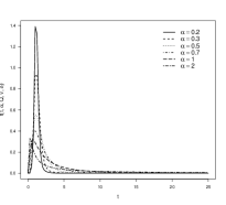
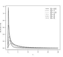
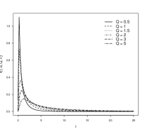
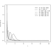
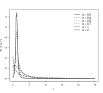
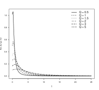
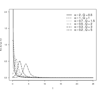
Figure 1 displays different shapes of the special cases of the QSBS distribution. We observe that as $q$ increases, the curves become flatter. We also observe that larger the value of $\alpha$, the heavier the tail of the distribution is.

(a) $\text{CN-BS}(\alpha,1,(0.2,0.2))$, $q=0.25$

(b) $\text{CN-BS}(1,Q,(0.2,0.2))$, $q=0.50$

(c) $\text{CN-BS}(\alpha,Q,(0.2,0.2))$, $q=0.75$

(d) $\text{SL-BS}(\alpha,1,2)$, $q=0.25$

(e) $\text{SL-BS}(1,Q,2)$, $q=0.50$

(f) $\text{SL-BS}(\alpha,Q,2)$, $q=0.75$

(g) $t_{\nu}\text{- BS}(\alpha,1,2)$, $q=0.25$

(h) $t_{\nu}\text{- BS}(1,Q,2)$, $q=0.50$

(i) $t_{\nu}\text{- BS}(\alpha,Q,2)$, $q=0.75$

Figure 1: PDFs for some QSBS family members considering different values of $\alpha$, $Q$ and $q=0.25,0.5,0.75,$ (in the lines) and for the models $t_{\nu}$-BS, SL-BS and CN-BS (in the columns), with $\bm{\nu}=2,2,(0.2,0.2)$, respectively.

3 QSBS quantile regression model

3.1 Model and EM algorithm

Let ${\bm{T}}=(T_{1},T_{2},\ldots,T_{n})^{\top}$ be a random sample of size $n$, where $T_{i}\sim\text{QSBS}(\alpha,Q_{i};H)$, for $i=1,2,\ldots,n$, and let $\bm{t}=(t_{1},t_{2},\ldots,t_{n})^{\top}$ denote the corresponding realization of $\bm{T}$. We propose a QSBS quantile regression model with structure for $Q_{i}$ expressed as

$$h(Q_{i})=\eta_{i}=\bm{x_{i}^{\top}\beta},\;i=1,2,\ldots,n,$$ (14)

where $h:\mathbb{R}^{+}\rightarrow\mathbb{R}^{+}$ is a strictly monotonic, positive and at least twice differentiable link function, $Q_{i}=h^{-1}(\bm{x_{i}^{\top}\beta})$, $\bm{x}_{i}^{\top}=(1,x_{i1},\ldots,x_{ip})$ is the vector of covariates (fixed and known), and $\bm{\beta}=(\beta_{0},\beta_{1},\ldots,\beta_{p})^{\top}$ is the corresponding vector of regression coefficients.

We can implement the EM algorithm (Dempster et al.,, 1977) to obtain the ML estimate of $\bm{\theta}=(\alpha,\bm{\beta})^{\top}$. The parameter $\bm{\nu}$ that indexes the PDF of $h_{U}(\cdot)$ will be estimated using the profile log-likelihood. Specifically, Let ${\bm{t}}=(t_{1},\ldots,t_{n})^{\top}$ and ${\bm{u}}=(u_{1},\ldots,u_{n})^{\top}$ be the observed and missing data, respectively, with ${\bm{T}}=(T_{1},T_{2},\ldots,T_{n})^{\top}$ and ${\bm{U}}=(U_{1},U_{2},\ldots,U_{n})^{\top}$ being their corresponding random vectors. Thus, the complete data vector is written as ${\bm{y}}_{c}=({\bm{t}}^{\top},{\bm{u}}^{\top})^{\top}$. From Proposition 3,

$$T_{i}|U_{i}=u_{i} \overset{\text{ind.}}{\sim} \text{QBS}(\alpha_{u},Q_{i}),$$ (15)

$$U_{i} \overset{\text{ind.}}{\sim} h_{U}(u_{i}),\;i=1,2,\ldots,n,$$ (16)

where QBS denotes the BS distribution reparameterized by the quantile proposed by Sánchez et al., (2020) and $\alpha_{u}=\sqrt{g(u)}\alpha$. The complete data log-likelihood function for the QSBS quantile regression model associated with ${\bm{y}}_{c}=({\bm{t}}^{\top},{\bm{u}}^{\top})^{\top}$ is given by

$$\ell_{c}(\bm{\theta};\bm{t_{c}}) \propto -n\log(\alpha\gamma_{\alpha})-\frac{1}{2}\sum_{i=1}^{n}\log(Q_{i})+\sum_{i=1}^{n}\log\left(\frac{\gamma_{\alpha}^{2}}{2}+\frac{2Q_{i}}{t_{i}}\right)$$ (17)

$$-\frac{2}{(\alpha\gamma_{\alpha})^{2}}\sum_{i=1}^{n}\frac{1}{g(u_{i})}\frac{Q_{i}}{t_{i}}\left(\frac{\gamma_{\alpha}^{2}t_{i}}{4Q_{i}}-1\right)^{2}.$$

By taking the expected value of the complete data log-likelihood function in (17), conditional on $\bm{U}=\bm{u}$, and letting $\widehat{u}_{i}=\textrm{E}[1/g(U_{i})|T_{i}=t_{i};\bm{\widehat{\theta}}]$, $i=1,2,\ldots,n$, which we obtain from (10), (11) and (13), we have

$$\mathcal{Q}(\bm{\theta};\bm{\widehat{\theta}}) \propto -n\log(\alpha\gamma_{\alpha})-\frac{1}{2}\sum_{i=1}^{n}\log(Q_{i})+\sum_{i=1}^{n}\log\left(\gamma_{\alpha}^{2}t_{i}+4Q_{i}\right)$$ (18)

$$-\frac{2}{(\alpha\gamma_{\alpha})^{2}}\sum_{i=1}^{n}\widehat{u}_{i}\frac{Q_{i}}{t_{i}}\left(\frac{\gamma_{\alpha}^{2}t_{i}}{4Q_{i}}-1\right)^{2}.$$

Then, the steps to obtain the ML estimates of $\bm{\theta}=(\alpha,\bm{\beta})^{\top}$ via the EM algorithm are given by

E-Step.

Compute $\widehat{u}_{i}$, given $\bm{\theta}=\bm{\widehat{\theta}}$, for $i=1,2,\ldots,n$.

M-Step.

Update $\bm{\widehat{\theta}}$ by maximizing $\mathcal{Q}(\bm{\theta};\bm{\widehat{\theta}})$ with respect to $\bm{\theta}$.

The maximization in M-Step can be performed by taking the derivative of Equation (18) with respect to $\bm{\theta}=(\alpha,\beta_{0},\ldots,\beta_{p})$ and then equating it to zero, thereby providing the likelihood equations. The partial derivatives of (18) with respect to $\bm{\theta}$ are given by

$$\frac{\partial\mathcal{Q}(\bm{\theta};\bm{\widehat{\theta}})}{\partial\alpha} = -n\left(\frac{\gamma_{\alpha}+\alpha\gamma^{\prime}_{\alpha}}{\alpha\gamma_{\alpha}}\right)+2\gamma_{\alpha}\gamma^{\prime}_{\alpha}\sum_{i=1}^{n}\frac{t_{i}}{\gamma^{2}_{\alpha}t_{i}+4Q_{i}}+\frac{1}{\alpha^{3}}\sum_{i=1}^{n}\widehat{u}_{i}\left[\frac{\gamma^{2}_{\alpha}t_{i}}{4Q_{i}}+\frac{4Q_{i}}{\gamma^{2}_{\alpha}t_{i}}-2\right]$$ (19)

$$-\frac{1}{\alpha^{2}}\sum_{i=1}^{n}\widehat{u}_{i}\left[\frac{\gamma_{\alpha}\gamma^{\prime}_{\alpha}t_{i}}{4Q_{i}}-\frac{4Q_{i}\gamma^{\prime}_{\alpha}}{\gamma^{3}_{\alpha}t_{i}}\right],$$

$$\frac{\partial\mathcal{Q}(\bm{\theta};\bm{\widehat{\theta}})}{\partial\beta_{j}} = \sum_{i=1}^{n}\left\{\left[-\frac{1}{2Q_{i}}+\frac{4}{\gamma^{2}_{\alpha}t_{i}+4Q_{i}}-\frac{\widehat{u}_{i}}{\alpha^{2}}\left(-\frac{\gamma_{\alpha}^{2}t_{i}}{8Q_{i}^{2}}+\frac{2}{\gamma_{\alpha}^{2}t_{i}}\right)\right]\left(\frac{\partial Q_{i}}{\partial\eta_{i}}\right)\left(\frac{\partial\eta_{i}}{\partial\beta_{j}}\right)\right\},$$ (20)

for $j=0,1,\ldots,p$, where $\gamma^{\prime}_{\alpha}=y_{q}+\alpha y_{q}^{2}/\sqrt{(\alpha y_{q})^{2}+4}$ is the first derivative of $\gamma_{\alpha}$ with respect to $\alpha$. The system of equations are solved using the BFGS quasi-Newton method; see Jamshidian and Jennrich, (1997); McLachlan and Krishnan, (2007). The convergence of the EM algorithm can be established using the following stopping criterion: $|\mathcal{Q}(\bm{\theta}^{(r+1)};\bm{\widehat{\theta}}^{(r)})-\mathcal{Q}(\bm{\theta}^{(r)};\bm{\widehat{\theta}}^{(r)})|<\varepsilon$, where $\varepsilon$ is a prespecified tolerance level; see McLachlan and Krishnan, (2007). Starting values are required to initiate the EM procedure, namely, $\widehat{\alpha}^{(0)},\widehat{\beta}_{0}^{(0)},\ldots,\widehat{\beta}_{p}^{(0)}$. These can be obtained from the work of Rieck and Nedelman, (1991).

A disadvantage of the EM algorithm in relation to Newton-type methods is that we cannot obtain the estimates of the standard errors directly through the Fisher information matrix. There are several approaches proposed to obtain the standard errors of ML estimators; see, for example, Baker, (1992), Oakes, (1999) and Louis, (1982), among others. The approach developed by Louis, (1982) is based on the missing information principle. In this method, the score function of the incomplete data log-likelihood function is related to the conditional expectation of the complete data log-likelihood function as follows: $S_{o}(\bm{y};\bm{\theta})=\textrm{E}[\partial\ell_{c}(\bm{\theta};\bm{t})/\partial\bm{\theta}]$, where $S_{o}(\bm{y};\bm{\theta})=\partial\ell_{o}(\bm{\theta};\bm{t})/\partial\bm{\theta}$ and $S_{c}(\bm{y};\bm{\theta})=\partial\ell_{c}(\bm{\theta};\bm{t})/\partial\bm{\theta}$ are the score functions of the incomplete data and complete data, respectively. Meilijson, (1989) presents a definition of the empirical information matrix as follows:

$$\text{I}_{e}(\bm{\theta};\bm{t})=\sum_{i=1}^{n}s(t_{i};\bm{\theta})s^{\top}(t_{i};\bm{\theta})-\frac{1}{n}S(\bm{t};\bm{\theta})S^{\top}(\bm{t};\bm{\theta}),$$

such that $S(\bm{t};\bm{\theta})=\sum_{i=1}^{n}s(t_{i},\bm{\theta})$ and $s(t_{i},\bm{\theta})$ is called the empirical score function of the $i$-th observation, $i=1,2,\ldots,n$. Replacing $\bm{\theta}$ with its respective ML estimates $\bm{\widehat{\theta}}$, we obtain $S(\bm{t};\bm{\widehat{\theta}})=0$. Then, the empirical information matrix is given by

$$\text{I}_{e}(\bm{\widehat{\theta}};\bm{t})=\sum_{i=1}^{n}s(t_{i};\bm{\widehat{\theta}})^{(r)}s^{\top}(t_{i};\bm{\widehat{\theta}})^{(r)},$$

where $s(t_{i};\bm{\widehat{\theta}})^{(r)}$ is the empirical score function obtained in the $r$-th iteration using the EM algorithm, that is,

$$s(t_{i};\bm{\widehat{\theta}})^{(r)}=\textrm{E}[s(t_{i},u_{i}^{(r)};\bm{\theta}^{(r)})|t_{i}],$$

where $u_{i}^{(r)}$ is the latent variable obtained in the $r$-th iteration with conditional distribution $h_{U|T}(u_{i}|t_{i})$ and the partial derivatives of the complete data log-likelihood function in relation to $\alpha$ and $\bm{\beta}$ are given, respectively, by (19) and (20).

By the method of Louis, (1982), an approximation to the observed information matrix observed at the $r$-th iteration can be obtained as $\text{I}_{e}(\bm{\widehat{\theta}};\bm{t})^{(r)}=\sum_{i=1}^{n}s(t_{i};\bm{\widehat{\theta}})^{(r)}s^{\top}(t_{i};\bm{\widehat{\theta}})^{(r)}$. Therefore, an approximation of the variance-covariance matrix is obtained by inverting the empirical Fisher information matrix $\text{I}_{e}(\bm{\widehat{\theta}};\bm{t})^{(r)}$ after convergence.

We estimate the extra parameter $\nu$ (or extra parameter vector $\bm{\nu}$) by using the profile log-likelihood approach. First, we compute the ML estimate of $\bm{\theta}$ by using the EM algorithm, for each $\nu\in\{a,\ldots,b\}$, where $a$ and $b$ are predefined limits, then the final estimate of $\nu$ is the one that maximizes the log-likelihood function and the associated estimate of $\bm{\theta}$ is then the final one; see Saulo et al., (2021). The extra parameter is estimated through the profile log-likelihood approach because it provides robustness to outlying observations under Student-$t$ models. According to Lucas, (1997), the robustness only holds if the degree of freedom is fixed rather than directly estimated in the maximization of the log-likelihood function. Moreover, some difficulties in computing the extra parameter can be found in other models.

3.2 Residual Analysis

Residuals are important tools to assess goodness-of-fit and departures from the assumptions of the postulated model. In particular, the generalized Cox-Snell (GCS) and randomized quantile (RQ) residuals are widely used for these purposes; see Lee and Wang, (2003), Dasilva et al., (2020) and Saulo et al., (2022). The GCS and RQ residuals are respectively given by

$$\widehat{r}_{i}^{\text{GCS}}=-\log[1-\widehat{\Phi}_{\text{SMN}}(a(t))]$$

and

$$\widehat{r}_{i}^{\text{RQ}}=\Phi^{-1}[\Phi_{\text{SMN}}(a(t))],$$

for $i=1,2,\ldots,n,$ where $\widehat{\Phi}_{\text{SMN}}(a(t))$ is the CDF of $T\sim\text{QSBS}(\widehat{\alpha},\bm{\widehat{\beta}},\bm{\nu})$ fitted to the data, and $\Phi(\cdot)^{-1}$ is the standard normal quantile function. These residuals have asymptotically standard exponential and standard normal distributions when the model is correctly specified. For both residuals, the distributional assumption can be verified using graphical techniques, hypothesis tests and descriptive statistics.

3.3 Hypothesis testing

We consider here the Wald, score, likelihood ratio and gradient statistical tests for the QSBS quantile regression model; see Terrell, (2002) and Saulo et al., (2022, 2021). Consider ${\bm{\theta}}$ to be a $p$-dimensional vector of parameters that index a QSBS quantile regression model. Assume our interest lies in testing the hypothesis ${\cal{H}}_{0}:{\bm{\theta}}_{1}={\bm{\theta}}^{(0)}_{1}$ against ${\cal{H}}_{1}:{\bm{\theta}}_{1}\neq{\bm{\theta}}^{(0)}_{1}$, where ${\bm{\theta}}=({\bm{\theta}}^{\top}_{1},{\bm{\theta}}^{\top}_{2})^{\top}$, ${\bm{\theta}}_{1}$ is a $r\times 1$ vector of parameters of interest and ${\bm{\theta}}_{2}$ is a $(p-r)\times 1$ vector of nuisance parameters. Then, the Wald (W), score (R), likelihood ratio (LR) and gradient (T) statistics are given, respectively, by

$$S_{W} = (\bm{\widehat{\theta}}-\widetilde{\bm{\theta}})^{\top}\mathcal{J}(\bm{\widehat{\theta}})(\bm{\widehat{\theta}}-\widetilde{\bm{\theta}}),$$

$$S_{R} = S(\widetilde{\bm{\theta}})^{\top}\mathcal{J}(\widetilde{\bm{\theta}})^{-1}S(\widetilde{\bm{\theta}}),$$

$$S_{LR} = -2[\ell(\widetilde{\bm{\theta}})-\ell(\bm{\widehat{\theta}})],$$

$$S_{T} = S(\widetilde{\bm{\theta}})^{\top}(\bm{\widehat{\theta}}-\widetilde{\bm{\theta}}),$$

where $\ell(\cdot)$ is the log-likelihood function, $S(\cdot)$ is the score function, $\mathcal{J}(\cdot)$ is the Fisher information matrix, and $\widehat{\bm{\theta}}=(\widehat{\bm{\theta}}^{\top}_{1},\widehat{\bm{\theta}}^{\top}_{2})^{\top}$ and $\widetilde{\bm{\theta}}=({\bm{\theta}}^{(0)\top}_{1},\widetilde{\bm{\theta}}^{\top}_{2})^{\top}$ are the unrestricted and restricted ML estimators of ${\bm{\theta}}$, respectively. In particular, we use the EM algorithm to obtain the ML estimates. The log-likelihood function in the $S_{LR}$ statistic is replaced by the expected value of the complete data log-likelihood function. Moreover, for the $S_{W}$ , $S_{R}$ and $S_{T}$ statistics, the score function and Fisher information matrix are approximated using their respective empirical versions presented in Subsection 3.1. In regular cases, we have, under ${\cal{H}}_{0}$ and as $n\rightarrow\infty$, the Wald, score, likelihood ratio and gradient statistical tests converging in distribution to $\chi^{2}_{r}$. We then reject ${\cal{H}}_{0}$ at nominal level $\alpha$ if the test statistic is larger than $\chi^{2}_{1-\alpha,r}$, the upper $\alpha$ quantile of the $\chi^{2}_{r}$ distribution.

4 Monte Carlo simulation

In this section, the results from two Monte Carlo simulation studies are presented. In the first study, we evaluate the performances of the EM algorithm for ML estimation and residuals. In the second study, we evaluate the performances of the aforementioned statistical tests. The simulations were performed using the R software; see R Core Team, (2020). The simulation scenario considers sample size $n=\{50,100,200\}$ and quantiles $q=\{0.25,0.5,0.75\}$, with a logarithmic link function for $Q_{i}$, and 5,000 Monte Carlo replications.

4.1 ML estimation and model selection

In this study, the data generating model has two covariates and is given by

$$\log(Q_{i})=\beta_{0}+\beta_{1}x_{1i}+\beta_{2}x_{2i},\,i=1,\ldots,n,$$ (21)

where $x_{1}$ and $x_{2}$ are covariates obtained from a uniform distribution in the interval (0,1), $\beta_{0}=2.5$, $\beta_{1}=3$ and $\beta_{2}=0.9$. Moreover, the simulation scenario considers shape parameters $\alpha=0.2,0.5,1.0$ and extra parameters $\bm{\nu}=(0.1,0.3)$ (CN-BS), $\nu=4$ (SL-BS) and $\nu=11$ ($t_{\nu}$-BS). The response observations, $t_{1},\ldots,t_{n}$, are then generated by using (7) and (21).

We evaluate the performance of the EM algorithm for obtaining the ML estimates using the bias, mean square error (MSE) and coverage probability (CP) of 95% asymptotic confidence interval. The Monte Carlo estimates of these quantities are given, respectively, by

$$\text{Bias}(\widehat{\varphi}) = \frac{1}{M}\sum_{r=1}^{M}(\widehat{\varphi}^{(r)}-\varphi),\,$$

$$\text{MSE}(\widehat{\varphi}) = \frac{1}{M}\sum_{r=1}^{M}(\widehat{\varphi}^{(r)}-\varphi)^{2},\,$$

$$\text{CP}(\widehat{\varphi}) = \frac{1}{M}\sum_{r=1}^{M}I(\varphi\in[\widehat{\varphi}_{L}^{(r)},\widehat{\varphi}_{U}^{(r)}]),$$

where $M$ is the number of Monte Carlo replications, $\varphi$ is the true parameter, $\widehat{\varphi}^{(r)}$ is the $r$-th ML estimate of $\varphi$, and $I(\cdot)$ is an indicator function of $\varphi$ belonging to the $r$-th asymptotic interval $[\widehat{\varphi}_{L}^{(r)},\widehat{\varphi}_{U}^{(r)}]$ with $\widehat{\varphi}_{L}^{(r)}$ and $\widehat{\varphi}_{U}^{(r)}$ denoting the lower and upper bounds, respectively.

In addition to analyzing the performance of the EM algorithm, this Monte Carlo simulation study also investigates the empirical distribution of the GCS and RQ residuals, which are assessed by the empirical mean (MN), median (MD), standard deviation (SD), coefficient of skewness (CS) and coefficient of (excess) kurtosis (CK).

Table 2 reports the empirical bias, MSE and CP for the quantile regression models based on the SL-BS distributions (due to space limitations we do not present the CN-BS and $t_{\nu}$-BS results). A look at the results in Table 2 allows us to conclude that as the sample size increases the bias and MSE both decreases, as one would expect. Moreover, these quantities increase as $\alpha$ increases. Finally, the CP approaches the 95% nominal level as the sample size increases.

Tables 3-4 present the empirical MN, MD, SD, CS and CK. Note that these values are expected to be 1, 0.69, 1, 2 and 6, respectively, for the GCS residuals, and 0, 0, 1, 0 and 0, respectively, for the RQ residuals. From Tables 3-4, note that for the CN-BS and $t_{\nu}$-BS cases, as the sample size increases the values of the empirical MN, MD, SD, CS and CK approaches these values of the reference EXP(1) and N(0,1) distributions. Therefore, the GCS and RQ residuals conform well with the reference distributions for the CN-BS and $t_{\nu}$-BS cases. Nevertheless, in the results of the SL-BS model the considered residuals do not conform well with the reference distributions.

Table 2: Empirical bias, MSE and CP from simulated data for the indicated ML estimates of the SL-BS quantile regression model ($\nu=4$).

$n=50$ $n=100$ $n=200$ $\alpha$ $q$ Bias MSE CP Bias MSE CP Bias MSE CP 0.2 0.25 $\widehat{\alpha}$ -0.0063 0.0005 0.9536 -0.0035 0.0002 0.9502 -0.0016 0.0001 0.9460 $\widehat{\beta}_{0}$ 0.0035 0.0067 0.9258 0.0041 0.0051 0.9338 0.0007 0.0018 0.9452 $\widehat{\beta}_{1}$ 0.0010 0.0105 0.9478 -0.0014 0.0067 0.9472 -0.0003 0.0033 0.9448 $\widehat{\beta}_{2}$ 0.0008 0.0131 0.9516 -0.0015 0.0061 0.9462 0.0008 0.0031 0.9504 0.5 $\widehat{\alpha}$ -0.0072 0.0005 0.9542 -0.0033 0.0002 0.9498 -0.0019 0.0001 0.9530 $\widehat{\beta}_{0}$ -0.0013 0.0067 0.9198 -0.0006 0.0037 0.9382 -0.0003 0.0023 0.9422 $\widehat{\beta}_{1}$ 0.0035 0.0118 0.9456 0.0016 0.0067 0.9500 -0.0001 0.0037 0.9506 $\widehat{\beta}_{2}$ -0.0001 0.0117 0.9468 0.0000 0.0068 0.9516 0.0008 0.0033 0.9472 0.75 $\widehat{\alpha}$ -0.0071 0.0005 0.9470 -0.0036 0.0002 0.9522 -0.0017 0.0001 0.9540 $\widehat{\beta}_{0}$ -0.0041 0.0107 0.9212 -0.0038 0.0033 0.9316 -0.0013 0.0018 0.9418 $\widehat{\beta}_{1}$ -0.0017 0.0176 0.9496 0.0003 0.0064 0.9470 -0.0002 0.0031 0.9522 $\widehat{\beta}_{2}$ -0.0020 0.0140 0.9498 0.0005 0.0067 0.9486 -0.0006 0.0031 0.9554 0.5 0.25 $\widehat{\alpha}$ -0.0180 0.0031 0.9486 -0.0096 0.0015 0.9514 -0.0044 0.0007 0.9504 $\widehat{\beta}_{0}$ 0.0158 0.0421 0.9244 0.0074 0.0228 0.9346 0.0039 0.0108 0.9392 $\widehat{\beta}_{1}$ -0.0068 0.0647 0.9404 0.0012 0.0327 0.9464 -0.0007 0.0178 0.9506 $\widehat{\beta}_{2}$ 0.0034 0.0734 0.9568 0.0001 0.0382 0.9494 0.0012 0.0193 0.9484 0.5 $\widehat{\alpha}$ -0.0183 0.0031 0.9538 -0.0083 0.0015 0.9508 -0.0043 0.0007 0.9552 $\widehat{\beta}_{0}$ -0.0013 0.0459 0.9170 0.0004 0.0282 0.9356 0.0004 0.0119 0.9354 $\widehat{\beta}_{1}$ -0.0006 0.0813 0.9506 -0.0009 0.0383 0.9530 -0.0004 0.0208 0.9520 $\widehat{\beta}_{2}$ -0.0015 0.0649 0.9492 0.0002 0.0427 0.9548 -0.0001 0.0180 0.9446 0.75 $\widehat{\alpha}$ -0.0182 0.0030 0.9460 -0.0087 0.0014 0.9508 -0.0049 0.0007 0.9516 $\widehat{\beta}_{0}$ -0.0122 0.0671 0.9264 -0.0075 0.0264 0.9378 -0.0048 0.0108 0.9432 $\widehat{\beta}_{1}$ 0.0009 0.0893 0.9442 0.0006 0.0456 0.9514 -0.0015 0.0164 0.9522 $\widehat{\beta}_{2}$ -0.0047 0.0767 0.9504 0.0030 0.0353 0.9466 0.0029 0.0190 0.9484 1 0.25 $\widehat{\alpha}$ -0.0414 0.0127 0.9616 -0.0206 0.0061 0.9580 -0.0103 0.0029 0.9530 $\widehat{\beta}_{0}$ 0.0278 0.1608 0.9196 0.0120 0.0731 0.9284 0.0081 0.0361 0.9442 $\widehat{\beta}_{1}$ 0.0031 0.2456 0.9554 0.0035 0.1498 0.9566 -0.0028 0.0620 0.9524 $\widehat{\beta}_{2}$ 0.0041 0.2423 0.9606 0.0039 0.1439 0.9580 0.0017 0.0641 0.9536 0.5 $\widehat{\alpha}$ -0.0372 0.0129 0.9680 -0.0177 0.0057 0.9580 -0.0086 0.0029 0.9536 $\widehat{\beta}_{0}$ -0.0057 0.1361 0.9200 -0.0002 0.0736 0.9388 0.0025 0.0385 0.9394 $\widehat{\beta}_{1}$ -0.0088 0.2754 0.9582 -0.0013 0.1190 0.9532 -0.0064 0.0595 0.9524 $\widehat{\beta}_{2}$ 0.0192 0.2526 0.9618 0.0037 0.1142 0.9554 0.0013 0.0621 0.9528 0.75 $\widehat{\alpha}$ -0.0398 0.0130 0.9634 -0.0170 0.0059 0.9544 -0.0091 0.0029 0.9528 $\widehat{\beta}_{0}$ -0.0289 0.1368 0.9158 -0.0088 0.0708 0.9372 -0.0096 0.0337 0.9446 $\widehat{\beta}_{1}$ -0.0062 0.2156 0.9482 -0.0076 0.1237 0.9532 -0.0001 0.0592 0.9492 $\widehat{\beta}_{2}$ 0.0062 0.2486 0.9608 -0.0019 0.1315 0.9524 0.0053 0.0575 0.9542

Table 3: Summary statistics for the GCS residuals.

$n=50$ $n=100$ $n=200$ $\alpha$ $q$ CN-BS SL-BS $t_{\nu}$-BS CN-BS SL-BS $t_{\nu}$-BS CN-BS SL-BS $t_{\nu}$-BS 0.2 0.25 MN 1.0007 0.2249 1.0002 1.0003 3.4373 1.0000 1.0002 2.7172 1.0001 MD 0.6980 0.0000 0.6964 0.6956 0.7111 0.6952 0.6941 0.2370 0.6940 SD 1.0008 0.7546 1.0007 0.9994 4.4814 0.9993 1.0000 3.8889 0.9998 CS 1.6378 4.0803 1.6428 1.7848 1.0108 1.7883 1.8767 1.2936 1.8774 CK 3.1251 17.7753 3.1549 4.1353 -0.4425 4.1577 4.8594 0.4671 4.8577 0.5 MN 1.0004 6.9641 0.9999 1.0003 1.1698 1.0000 1.0002 2.8319 1.0001 MD 0.6974 4.5335 0.6968 0.6956 0.0004 0.6952 0.6941 0.5567 0.6940 SD 0.9997 6.6111 0.9995 0.9994 2.5135 0.9993 1.0000 3.8723 0.9999 CS 1.6322 0.5019 1.6373 1.7848 2.3886 1.7883 1.8767 1.2494 1.8774 CK 3.0959 -1.2344 3.1217 4.1354 4.9818 4.1578 4.8594 0.3308 4.8576 0.75 MN 1.0004 3.4180 0.9999 1.0003 5.4234 1.0000 1.0002 13.7272 1.0001 MD 0.6974 1.1057 0.6968 0.6956 3.1935 0.6952 0.6941 14.9827 0.6940 SD 0.9997 4.3039 0.9995 0.9994 5.6753 0.9993 1.0000 6.0437 0.9999 CS 1.6322 0.9856 1.6373 1.7849 0.5817 1.7883 1.8768 -0.5336 1.8774 CK 3.0961 -0.4622 3.1218 4.1356 -1.1559 4.1579 4.8596 -0.6473 4.8578 0.5 0.25 MN 1.0002 6.2318 0.9996 1.0001 5.0268 0.9998 1.0001 1.0149 1.0000 MD 0.6976 5.4538 0.6970 0.6957 3.8996 0.6953 0.6941 0.2530 0.6939 SD 0.9978 4.8210 0.9976 0.9984 4.3076 0.9983 0.9995 1.6239 0.9993 CS 1.6229 0.4127 1.6271 1.7793 0.6738 1.7821 1.8734 2.3450 1.8738 CK 3.0526 -1.0874 3.0718 4.1048 -0.6312 4.1224 4.8365 6.2482 4.8344 0.5 MN 1.0001 3.4666 0.9996 1.0001 3.4666 0.9998 1.0001 3.2460 1.0000 MD 0.6976 2.4009 0.6970 0.6957 2.4009 0.6953 0.6941 2.0450 0.6939 SD 0.9978 3.3556 0.9976 0.9984 3.3556 0.9983 0.9995 3.3414 0.9993 CS 1.6229 0.9513 1.6271 1.7793 0.9513 1.7821 1.8734 1.1899 1.8738 CK 3.0526 0.0021 3.0717 4.1049 0.0021 4.1224 4.8366 0.6885 4.8344 0.75 MN 1.0001 1.3331 0.9996 1.0001 0.7800 0.9998 1.0001 2.4466 1.0000 MD 0.6976 0.4540 0.6970 0.6957 0.2002 0.6953 0.6941 1.0708 0.6939 SD 0.9978 1.9673 0.9976 0.9984 1.3305 0.9983 0.9995 3.0264 0.9993 CS 1.6229 1.9690 1.6271 1.7794 2.6832 1.7822 1.8734 1.4214 1.8738 CK 3.0527 3.8322 3.0718 4.1049 8.5732 4.1224 4.8366 1.2562 4.8345 1 0.25 MN 0.9993 1.7884 0.9989 0.9997 0.8007 0.9994 0.9997 2.6806 0.9997 MD 0.6986 1.0537 0.6979 0.6961 0.3817 0.6957 0.6942 1.7059 0.6941 SD 0.9921 2.0649 0.9918 0.9956 1.1435 0.9953 0.9978 2.7691 0.9976 CS 1.5961 1.7839 1.5976 1.7637 2.6123 1.7642 1.8639 1.6326 1.8633 CK 2.9246 3.3013 2.9240 4.0165 8.8216 4.0183 4.7733 2.5941 4.7663 0.5 MN 0.9993 1.3375 0.9989 0.9997 1.4969 0.9994 0.9997 0.6229 0.9997 MD 0.6986 0.7459 0.6979 0.6961 0.8467 0.6957 0.6942 0.2700 0.6941 SD 0.9921 1.6592 0.9918 0.9956 1.8269 0.9953 0.9978 0.9235 0.9976 CS 1.5961 1.9805 1.5976 1.7637 2.0812 1.7642 1.8639 2.7777 1.8633 CK 2.9246 4.4033 2.9239 4.0165 5.0290 4.0183 4.7733 10.5620 4.7663 0.75 MN 0.9993 1.9122 0.9989 0.9997 3.4851 0.9994 0.9997 0.9887 0.9997 MD 0.6986 1.0797 0.6979 0.6961 2.3979 0.6957 0.6942 0.4844 0.6941 SD 0.9921 2.2636 0.9918 0.9956 3.2461 0.9953 0.9978 1.3787 0.9976 CS 1.5961 1.7622 1.5976 1.7637 1.2772 1.7642 1.8639 2.6184 1.8633 CK 2.9247 3.0441 2.9240 4.0165 1.1415 4.0184 4.7733 8.8776 4.7663

Table 4: Summary statistics for the RQ residuals.

$n=50$ $n=100$ $n=200$ $\alpha$ $q$ CN-BS SL-BS $t_{\nu}$-BS CN-BS SL-BS $t_{\nu}$-BS CN-BS SL-BS $t_{\nu}$-BS 0.2 0.25 MN -0.0007 3.6621 -0.0003 -0.0004 -0.0222 -0.0001 -0.0002 0.5812 -0.0002 MD -0.0018 4.4962 -0.0002 -0.0010 0.0091 -0.0007 -0.0002 0.8356 -0.0001 SD 1.0093 2.1911 1.0093 1.0045 3.1032 1.0044 1.0022 3.1333 1.0021 CS -0.0054 -0.9419 -0.0057 -0.0023 -0.0018 -0.0028 -0.0035 -0.1484 -0.0033 CK -0.2145 -0.1194 -0.2044 -0.1149 -1.4337 -0.1129 -0.0611 -1.4539 -0.0606 0.5 MN -0.0006 -2.1173 -0.0001 -0.0004 2.2921 -0.0001 -0.0002 0.2326 -0.0002 MD -0.0012 -2.2758 -0.0008 -0.0010 3.4442 -0.0007 -0.0002 0.2018 -0.0001 SD 1.0092 2.6909 1.0092 1.0045 2.8829 1.0044 1.0022 2.9603 1.0021 CS -0.0027 0.3635 -0.0030 -0.0023 -0.7669 -0.0028 -0.0035 -0.0082 -0.0033 CK -0.2150 -1.0596 -0.2074 -0.1149 -0.7860 -0.1129 -0.0611 -1.3435 -0.0606 0.75 MN -0.0006 -0.2725 -0.0001 -0.0004 -1.1287 -0.0001 -0.0002 -4.5000 -0.0002 MD -0.0012 -0.4018 -0.0008 -0.0010 -1.7211 -0.0007 -0.0002 -4.9832 -0.0001 SD 1.0092 2.8834 1.0092 1.0045 3.1633 1.0044 1.0022 1.5547 1.0021 CS -0.0027 0.0591 -0.0030 -0.0023 0.3594 -0.0029 -0.0035 1.2891 -0.0033 CK -0.2149 -1.3973 -0.2074 -0.1149 -1.2754 -0.1129 -0.0611 1.2414 -0.0606 0.5 0.25 MN -0.0006 -2.3923 -0.0001 -0.0004 -1.9300 -0.0001 -0.0001 0.7844 -0.0001 MD -0.0012 -2.5996 -0.0007 -0.0010 -2.0355 -0.0006 -0.0001 0.7682 0.0000 SD 1.0088 1.8164 1.0088 1.0042 1.8304 1.0042 1.0020 1.8929 1.0020 CS -0.0021 0.3022 -0.0023 -0.0023 0.2409 -0.0027 -0.0035 -0.0576 -0.0033 CK -0.2258 -1.0039 -0.2194 -0.1212 -0.8613 -0.1196 -0.0649 -0.7816 -0.0645 0.5 MN -0.0006 -0.2474 -0.0001 -0.0004 -1.2189 -0.0001 -0.0001 -1.1277 -0.0000 MD -0.0012 -0.3091 -0.0007 -0.0010 -1.3267 -0.0006 -0.0001 -1.1230 0.0000 SD 1.0088 1.9014 1.0088 1.0042 1.8326 1.0042 1.0020 1.7712 1.0020 CS -0.0021 0.1187 -0.0023 -0.0023 0.2699 -0.0027 -0.0035 0.0708 -0.0033 CK -0.2258 -0.7672 -0.2194 -0.1212 -0.6692 -0.1196 -0.0649 -0.6857 -0.0645 0.75 MN -0.0006 0.3435 -0.0001 -0.0004 0.9719 -0.0001 -0.0001 -0.4675 -0.0000 MD -0.0012 0.3910 -0.0007 -0.0010 0.9259 -0.0006 -0.0001 -0.3988 0.0000 SD 1.0088 1.8131 1.0088 1.0042 1.7567 1.0042 1.0020 1.9726 1.0020 CS -0.0021 -0.1176 -0.0023 -0.0023 -0.0706 -0.0027 -0.0035 -0.0207 -0.0033 CK -0.2258 -0.7264 -0.2194 -0.1212 -0.6657 -0.1196 -0.0649 -0.8315 -0.0645 1 0.25 MN -0.0007 -0.4018 -0.0002 -0.0004 0.5441 -0.0000 0.0000 -1.0096 0.0001 MD -0.0012 -0.3610 -0.0008 -0.0009 0.4899 -0.0007 0.0001 -0.9013 0.0002 SD 1.0071 1.4377 1.0074 1.0034 1.3864 1.0035 1.0016 1.4481 1.0016 CS -0.0004 -0.0746 -0.0004 -0.0020 0.1054 -0.0022 -0.0034 -0.2055 -0.0032 CK -0.2586 -0.2157 -0.2562 -0.1399 -0.0067 -0.1402 -0.0758 -0.2410 -0.0763 0.5 MN -0.0007 -0.0396 -0.0002 -0.0004 -0.1923 -0.0000 0.0000 0.8391 0.0001 MD -0.0012 -0.0447 -0.0008 -0.0009 -0.1726 -0.0007 0.0001 0.7316 0.0002 SD 1.0071 1.4219 1.0074 1.0034 1.4142 1.0035 1.0016 1.4253 1.0016 CS -0.0004 0.0318 -0.0004 -0.0020 -0.0342 -0.0022 -0.0034 0.2282 -0.0032 CK -0.2587 -0.0933 -0.2562 -0.1399 -0.0014 -0.1402 -0.0758 -0.1461 -0.0763 0.75 MN -0.0007 -0.4664 -0.0002 -0.0004 -1.4258 -0.0000 0.0000 0.3369 0.0001 MD -0.0012 -0.4011 -0.0008 -0.0009 -1.3223 -0.0007 0.0001 0.2991 0.0002 SD 1.0071 1.4966 1.0074 1.0034 1.4880 1.0035 1.0016 1.4284 1.0016 CS -0.0005 -0.1262 -0.0004 -0.0020 -0.1390 -0.0022 -0.0034 0.0640 -0.0032 CK -0.2586 -0.2693 -0.2562 -0.1399 -0.5011 -0.1402 -0.0758 0.0339 -0.0763

4.2 Hypothesis tests

We now present Monte Carlo simulation studies to evaluate the performances of the Wald, score, likelihood ratio and gradient tests. We considered two measures: null rejection rate (size) and non-null rejection rate (power). The data generating model has three covariates and is given by

$$\log(Q_{i})=\beta_{0}+\beta_{1}x_{1i}+\beta_{2}x_{2i}+\beta_{3}x_{3i},\;i=1,2,\ldots,n,$$

where the values of the coefficients $\beta_{j}$, $j=0,1,\ldots,3$, not fixed in $H_{0}$ are all equal to 1. The covariate values were obtained as U(0,1) random draws. The interest lies in testing $H_{0}:\beta_{3-\kappa+1}=\cdots=\beta_{3}=0$, with $\kappa=1,3$ against $H_{0}:\beta_{3-\kappa+1}=\cdots=\beta_{3}\neq 0$, with $\kappa=1,3$. The tests’ nominal levels used are $\alpha=0.01,0.05,0.1$.

Tables 5-7 present the simulation results of null rejection rates for $H_{0}:\beta_{3}=0$ and in the CN-BS, SL-BS and $t_{\nu}$-BS quantile regression models, respectively. From these tables, we observe that as the sample size increases the test sizes for all considered test statistics tends to approach their respective nominal values. In particular, the Wald and gradient statistics present null rejection rates closer to the nominal levels even for small sample sizes. Finally, in general, the tests’ null rejection rates do not seem to be affected by the shape parameter $\alpha$. Tables 12-14 (Appendix A) present the simulation results of null rejection rates for $H_{0}:\beta_{1}=\beta_{2}=\beta_{3}=0$ in the CN-BS, SL-BS and $t_{\nu}$-BS quantile regression models, respectively. Analogously to the case where $\kappa=1$, the tests’ null rejection rates does not change according to the value of $\alpha$ and the Wald and gradient statistics showed greater control over the error type I when compared to the other test statistics that we analyzed. On the other hand, the score statistic is the one with the highest null rejection rates among all considered test statistics.

Table 5: Null rejection rates for $H_{0}:\beta_{3}=0$ in the CN-BS quantile regression model ($\nu=0.1$, $\delta=0.3$).

$n=50$ $n=100$ $n=200$ $\alpha$ $q$ 1% 5% 10% 1% 5% 10% 1% 5% 10% 0.2 0.25 $S_{W}$ 0.0126 0.0516 0.1026 0.015 0.0566 0.1024 0.0078 0.0488 0.104 $S_{LR}$ 0.0214 0.0768 0.1324 0.0196 0.0728 0.126 0.012 0.0668 0.1262 $S_{R}$ 0.0386 0.108 0.1764 0.0204 0.0782 0.1356 0.0142 0.063 0.1232 $S_{T}$ 0.012 0.0618 0.1156 0.0114 0.0502 0.1038 0.01 0.0534 0.1026 0.5 $S_{W}$ 0.0126 0.0514 0.1026 0.015 0.0566 0.1022 0.0078 0.0488 0.1038 $S_{LR}$ 0.0186 0.0786 0.1386 0.0196 0.073 0.126 0.012 0.0668 0.1262 $S_{R}$ 0.0258 0.0894 0.1486 0.0198 0.074 0.1354 0.0116 0.06 0.1102 $S_{T}$ 0.0086 0.0486 0.1012 0.0082 0.0504 0.102 0.0126 0.0544 0.104 0.75 $S_{W}$ 0.0126 0.0514 0.1024 0.0148 0.0566 0.102 0.0078 0.049 0.1042 $S_{LR}$ 0.0186 0.0786 0.1386 0.0196 0.0728 0.126 0.012 0.0668 0.1262 $S_{R}$ 0.038 0.1068 0.1824 0.0198 0.0758 0.137 0.0164 0.0736 0.132 $S_{T}$ 0.0124 0.0544 0.1112 0.0088 0.0508 0.1012 0.0108 0.0506 0.1038 0.5 0.25 $S_{W}$ 0.013 0.0482 0.0964 0.0142 0.0554 0.1024 0.0074 0.0488 0.1014 $S_{LR}$ 0.0178 0.078 0.1374 0.02 0.0716 0.1252 0.0114 0.066 0.1236 $S_{R}$ 0.0378 0.1104 0.1834 0.0236 0.076 0.142 0.012 0.0602 0.1112 $S_{T}$ 0.0128 0.0592 0.111 0.0108 0.048 0.1018 0.0086 0.0526 0.094 0.5 $S_{W}$ 0.013 0.0482 0.0964 0.0142 0.0554 0.1024 0.0074 0.0488 0.1012 $S_{LR}$ 0.0178 0.078 0.1374 0.02 0.0716 0.1252 0.0114 0.066 0.1236 $S_{R}$ 0.0216 0.0834 0.1486 0.0202 0.0704 0.1236 0.0122 0.056 0.1056 $S_{T}$ 0.0062 0.0468 0.0982 0.0122 0.0518 0.1076 0.0092 0.0524 0.1044 0.75 $S_{W}$ 0.013 0.0482 0.0964 0.0142 0.0556 0.1024 0.0074 0.0488 0.1012 $S_{LR}$ 0.0178 0.078 0.1374 0.02 0.0716 0.1252 0.0114 0.066 0.1236 $S_{R}$ 0.0442 0.1186 0.1932 0.02 0.0716 0.1342 0.015 0.0668 0.118 $S_{T}$ 0.0144 0.0604 0.1122 0.0108 0.0556 0.1102 0.0134 0.0588 0.1158 1 0.25 $S_{W}$ 0.0108 0.0418 0.083 0.0122 0.05 0.0932 0.0062 0.046 0.098 $S_{LR}$ 0.018 0.0728 0.1322 0.0176 0.0632 0.116 0.011 0.0634 0.1168 $S_{R}$ 0.0424 0.1252 0.189 0.0256 0.0834 0.1422 0.0158 0.0624 0.1162 $S_{T}$ 0.0092 0.0544 0.1114 0.0084 0.0556 0.1104 0.0108 0.0494 0.1066 0.5 $S_{W}$ 0.0108 0.0418 0.083 0.0122 0.05 0.0932 0.0062 0.046 0.098 $S_{LR}$ 0.018 0.0728 0.1322 0.0178 0.0632 0.116 0.011 0.0634 0.1168 $S_{R}$ 0.0238 0.0898 0.1594 0.0182 0.0724 0.1286 0.0136 0.0582 0.1096 $S_{T}$ 0.0086 0.0484 0.1018 0.007 0.0444 0.0972 0.0096 0.0458 0.0928 0.75 $S_{W}$ 0.0108 0.0418 0.083 0.0122 0.05 0.0932 0.0062 0.046 0.098 $S_{LR}$ 0.018 0.0728 0.1322 0.0176 0.0632 0.116 0.011 0.0634 0.1168 $S_{R}$ 0.0384 0.1166 0.1834 0.021 0.0774 0.1342 0.012 0.06 0.1154 $S_{T}$ 0.013 0.0538 0.107 0.0112 0.0516 0.1052 0.0106 0.052 0.1066

Table 6: Null rejection rates for $H_{0}:\beta_{3}=0$ in the SL-BS quantile regression model ($\nu=4$).

$n=50$ $n=100$ $n=200$ $\alpha$ $q$ 1% 5% 10% 1% 5% 10% 1% 5% 10% 0.2 0.25 $S_{W}$ 0.0116 0.0478 0.0898 0.0112 0.0504 0.0996 0.0104 0.049 0.098 $S_{LR}$ 0.0146 0.064 0.122 0.0114 0.056 0.11 0.012 0.0534 0.1118 $S_{R}$ 0.0366 0.1116 0.1876 0.0234 0.0774 0.1334 0.0126 0.065 0.1178 $S_{T}$ 0.0078 0.0522 0.1034 0.0122 0.0554 0.106 0.0098 0.06 0.113 0.5 $S_{W}$ 0.0106 0.049 0.0908 0.0112 0.0502 0.0996 0.0104 0.049 0.098 $S_{LR}$ 0.017 0.0634 0.117 0.0124 0.0608 0.1112 0.0108 0.0484 0.1006 $S_{R}$ 0.0284 0.0926 0.1524 0.016 0.0672 0.1192 0.0106 0.051 0.1022 $S_{T}$ 0.0088 0.0452 0.0998 0.0102 0.05 0.1016 0.0102 0.0516 0.0966 0.75 $S_{W}$ 0.0106 0.049 0.0908 0.0112 0.0502 0.0996 0.0104 0.049 0.0978 $S_{LR}$ 0.0148 0.0672 0.1272 0.0116 0.0602 0.1114 0.0132 0.0534 0.1004 $S_{R}$ 0.031 0.098 0.1684 0.022 0.0766 0.1306 0.0148 0.0604 0.122 $S_{T}$ 0.0082 0.0506 0.108 0.0086 0.0482 0.1014 0.0114 0.052 0.0996 0.5 0.25 $S_{W}$ 0.01 0.0452 0.0852 0.0106 0.0486 0.098 0.0102 0.0482 0.097 $S_{LR}$ 0.0158 0.0668 0.1232 0.0122 0.0566 0.1082 0.01 0.053 0.1064 $S_{R}$ 0.0386 0.112 0.1766 0.0288 0.0892 0.15 0.0152 0.0608 0.1144 $S_{T}$ 0.0078 0.0486 0.0984 0.0092 0.0514 0.099 0.0086 0.047 0.1004 0.5 $S_{W}$ 0.01 0.0452 0.0852 0.0106 0.0486 0.098 0.012 0.0498 0.0918 $S_{LR}$ 0.0122 0.057 0.1136 0.0136 0.058 0.1162 0.0098 0.0502 0.0998 $S_{R}$ 0.0258 0.0884 0.1528 0.0168 0.0674 0.125 0.013 0.063 0.111 $S_{T}$ 0.008 0.0466 0.103 0.0076 0.0492 0.1016 0.009 0.0532 0.1022 0.75 $S_{W}$ 0.01 0.0452 0.0852 0.0106 0.0486 0.098 0.008 0.0446 0.0926 $S_{LR}$ 0.0142 0.059 0.1112 0.0126 0.0644 0.1264 0.0108 0.0562 0.1096 $S_{R}$ 0.0348 0.1076 0.182 0.0248 0.0836 0.145 0.0162 0.0606 0.1132 $S_{T}$ 0.0086 0.0522 0.108 0.0104 0.0492 0.1022 0.0102 0.045 0.0938 1 0.25 $S_{W}$ 0.0072 0.031 0.0696 0.0088 0.0422 0.0852 0.0076 0.0434 0.0926 $S_{LR}$ 0.014 0.0624 0.1206 0.0108 0.0546 0.1038 0.0088 0.0486 0.095 $S_{R}$ 0.0402 0.1184 0.1794 0.0196 0.073 0.1378 0.0178 0.0616 0.1146 $S_{T}$ 0.0084 0.051 0.1066 0.0124 0.0606 0.1114 0.0094 0.0528 0.1042 0.5 $S_{W}$ 0.0072 0.031 0.0696 0.0088 0.042 0.0852 0.0076 0.0434 0.0926 $S_{LR}$ 0.0108 0.053 0.1098 0.0144 0.0574 0.1122 0.011 0.0442 0.0944 $S_{R}$ 0.0246 0.0874 0.15 0.0186 0.0684 0.1252 0.013 0.0642 0.1162 $S_{T}$ 0.008 0.0474 0.0986 0.0076 0.0476 0.0998 0.008 0.047 0.0994 0.75 $S_{W}$ 0.0072 0.031 0.0696 0.0088 0.0422 0.0852 0.0076 0.0434 0.0926 $S_{LR}$ 0.0124 0.0568 0.1102 0.013 0.055 0.105 0.01 0.0454 0.0894 $S_{R}$ 0.0344 0.1048 0.1744 0.023 0.0816 0.1424 0.0144 0.0596 0.1218 $S_{T}$ 0.0104 0.0638 0.113 0.011 0.0524 0.1036 0.013 0.052 0.1066

Table 7: Null rejection rates for $H_{0}:\beta_{3}=0$ in the $t_{\nu}$-BS quantile regression model ($\nu=11$).

$n=50$ $n=100$ $n=200$ $\alpha$ $q$ 1% 5% 10% 1% 5% 10% 1% 5% 10% 0.2 0.25 $S_{W}$ 0.0126 0.0534 0.1036 0.0156 0.0546 0.1062 0.007 0.0502 0.1052 $S_{LR}$ 0.0162 0.0696 0.1296 0.0182 0.0664 0.123 0.0092 0.0598 0.1164 $S_{R}$ 0.0332 0.0966 0.1634 0.0204 0.0786 0.1428 0.014 0.0666 0.1222 $S_{T}$ 0.0096 0.0534 0.11 0.0086 0.0544 0.1032 0.0104 0.049 0.1054 0.5 $S_{W}$ 0.0126 0.0536 0.1038 0.0156 0.0546 0.1062 0.007 0.0502 0.1052 $S_{LR}$ 0.0162 0.0696 0.1296 0.0182 0.0662 0.123 0.0092 0.0598 0.1162 $S_{R}$ 0.021 0.0812 0.1446 0.015 0.0646 0.1208 0.0126 0.0568 0.107 $S_{T}$ 0.0086 0.048 0.101 0.0116 0.0484 0.1036 0.0122 0.0494 0.1054 0.75 $S_{W}$ 0.0126 0.0536 0.1038 0.0156 0.0546 0.1064 0.007 0.0502 0.1052 $S_{LR}$ 0.0162 0.0694 0.1296 0.0184 0.0662 0.1232 0.0092 0.0598 0.116 $S_{R}$ 0.0424 0.1118 0.1776 0.0202 0.0742 0.1394 0.0184 0.0676 0.1274 $S_{T}$ 0.0106 0.0548 0.1082 0.0102 0.0536 0.1028 0.0098 0.052 0.1052 0.5 0.25 $S_{W}$ 0.0124 0.0514 0.098 0.0138 0.056 0.1024 0.0066 0.0482 0.1046 $S_{LR}$ 0.016 0.0666 0.1274 0.0178 0.063 0.1216 0.0088 0.0576 0.1126 $S_{R}$ 0.032 0.1006 0.1736 0.0212 0.0748 0.14 0.0146 0.0578 0.1162 $S_{T}$ 0.012 0.0608 0.1174 0.0112 0.0562 0.1036 0.0104 0.0528 0.0974 0.5 $S_{W}$ 0.0124 0.0514 0.098 0.0138 0.056 0.1024 0.0066 0.0482 0.1046 $S_{LR}$ 0.016 0.0666 0.1274 0.0178 0.063 0.1216 0.0088 0.0576 0.1126 $S_{R}$ 0.0218 0.084 0.1466 0.0144 0.063 0.1178 0.01 0.0576 0.1072 $S_{T}$ 0.0092 0.053 0.1026 0.0114 0.0504 0.1034 0.0098 0.051 0.098 0.75 $S_{W}$ 0.0124 0.0514 0.098 0.0138 0.056 0.1024 0.0066 0.0482 0.1046 $S_{LR}$ 0.016 0.0666 0.1274 0.0178 0.063 0.1216 0.0088 0.0576 0.1126 $S_{R}$ 0.0326 0.103 0.1688 0.018 0.069 0.1326 0.0126 0.0648 0.1234 $S_{T}$ 0.0106 0.0576 0.1136 0.0146 0.0586 0.105 0.0104 0.0528 0.1044 1 0.25 $S_{W}$ 0.0104 0.0426 0.0846 0.012 0.051 0.0952 0.0064 0.0438 0.0992 $S_{LR}$ 0.0136 0.063 0.123 0.0154 0.0584 0.1144 0.0078 0.0508 0.1072 $S_{R}$ 0.0338 0.1046 0.1722 0.0196 0.0744 0.1364 0.0124 0.0592 0.1208 $S_{T}$ 0.0112 0.0586 0.1092 0.012 0.0526 0.1014 0.0112 0.0548 0.1054 0.5 $S_{W}$ 0.0104 0.0426 0.0846 0.012 0.051 0.0952 0.0064 0.0438 0.0992 $S_{LR}$ 0.0136 0.063 0.123 0.0154 0.0584 0.1144 0.0078 0.0508 0.1072 $S_{R}$ 0.0246 0.0888 0.1424 0.0188 0.0654 0.1188 0.0122 0.0566 0.1104 $S_{T}$ 0.007 0.0498 0.1016 0.0094 0.0492 0.1016 0.0108 0.0502 0.1028 0.75 $S_{W}$ 0.0104 0.0426 0.0846 0.012 0.051 0.0952 0.0064 0.0438 0.0992 $S_{LR}$ 0.0136 0.063 0.123 0.0154 0.0584 0.1144 0.0078 0.0508 0.1072 $S_{R}$ 0.036 0.1148 0.1822 0.025 0.0818 0.1356 0.014 0.0632 0.1212 $S_{T}$ 0.0124 0.0582 0.1082 0.012 0.0568 0.1076 0.0096 0.047 0.1002

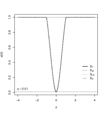
Figure 2 displays the test power curves for the CN-BS, SL-BS and $t_{\nu}$-BS models considering the hypotheses $H_{0}:\beta_{3-\kappa+1}=\ldots=\beta_{3}=0$ against $H_{1}:\beta_{3-\kappa+1}=\ldots=\beta_{3}=\delta$ with $|\delta|=0,1,2,3,4$ and $\kappa=1,3$, where $\pi(\delta)$ denotes the power function. The significance level considered was 1% with $n=100$ and $q=0.5$ (other settings present similar results). From this figure, we observe that there are no changes in the power performances of the tests, as well as for any of the CN-BS, SL-BS and $t_{\nu}$-BS models, so that we have $\pi(\delta)=1$ for $|\delta|\geq 1$.

(a) CN-BS, $\kappa=1$

(b) SL-BS, $\kappa=1$

(c) $t_{\nu}$-BS, $\kappa=1$

(d) CN-BS, $\kappa=3$

(e) SL-BS, $\kappa=3$

(f) $t_{\nu}$-BS, $\kappa=3$

Figure 2: Power curves of the $S_{W},S_{LR},S_{R}$ and $S_{T}$ tests for the CN-BS, SL-BS and $t_{\nu}$-BS quantile regression models (nominal level = 1%, $n=100$, $q=0.5$).

5 Application to personal accident insurance data

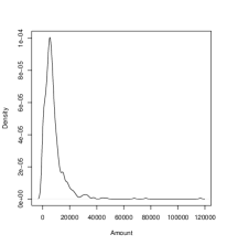
QSBS quantile regression models are now used to analyze a data set related to the personal injury insurance claims that correspond to amounts of paid money by an insurance policy in Australian dollars (response variable, amount). The data is collected from 767 individuals and the claims occurred between January 1998 and January 1999; see De Jong et al., (2008). The covariates considered in the study are: optime, denoting the operating time in percentage; legrep, with (1) or without (0) legal representation; and month, denoting the month of accident occurrence. Due to lack of correlation between the covariate month and the response variable amount, we removed this covariate from our analysis.

Table 8: Summary statistics for the personal accident insurance data.

MN	MD	SD	CV	CS	CK	Range	Min	Max	$n$
7820.59	6000	8339.26	106.63%	5.09	47.77	116556.7	30	116586.7	767

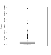
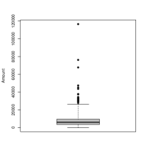
Table 8 reports the descriptive statistics of the observed amounts of paid money that includes MN, MD, SD, coefficient of variation (CV), CS, CK (excess) and range. From this table, we observe skewed and high kurtosis features in the data. Figure 3(a) confirms the skewness observed in Table 8. Figure 3(b) displays the usual and adjusted boxplots (Saulo et al.,, 2019), where the latter is useful when the data is distributed as skewedd. Note that the adjusted boxplot indicates that some potential outliers identified by the usual boxplot are not outliers.

(a) Density estimate

(b) Usual boxplot

(c) Adjusted boxplot

Figure 3: Density estimate and boxplots for the personal accident insurance data.

We then analyze the personal accident insurance data using the QSBS quantile regression model, expressed as

$$\log(Q_{i})=\beta_{0}+\beta_{1}\texttt{optime}+\beta_{2}\texttt{legrep},\;i=1,2,\ldots,767.$$ (22)

Table 9 reports the the averages of the AIC, BIC, AICc and HQIC values based on $q\in\{0.01,0.02,\ldots,0.99\}$ for the CN-BS, SL-BS and $t_{\nu}$-BS quantile regression models. The results indicate that the lowest values of AIC, BIC, AICc and HQIC are those based on the CN-BS model. Figure 4 displays the estimates of the CN-BS model parameters across $q\in\{0.01,0.02,\ldots,0.99\}$. From this figure, we observe that the estimate of $\beta_{0}$ tends to increase with an increase in $q$. Moreover, the estimates of ${\beta}_{1}$, ${\beta}_{2}$, $\alpha$ and $\nu$ present a cyclic behavior. These results show the relevance of considering a quantile approach rather than traditional mean/median approaches.

Table 9: Averages of the AIC, BIC, AICc and HQIC values based on $q\in\{0.01,0.02,\ldots,0.99\}$ for different models for the personal accident insurance data.

Model	AIC	BIC	AICc	HQIC
CN-BS	8204.634	8223.204	8204.686	8211.781
SL-BS	8220.061	8238.631	8220.114	8227.209
$t_{\nu}$-BS	8213.111	8231.681	8213.163	8220.259

(a) $\widehat{\beta}_{0}$

(b) $\widehat{\beta}_{1}$

(c) $\widehat{\beta}_{2}$

(d) $\widehat{\alpha}$

(e) $\widehat{\nu}$

(f) $\widehat{\delta}$

Figure 4: Estimated parameters in the CN-BS quantile regression models across $q$ for the personal accident insurance data.

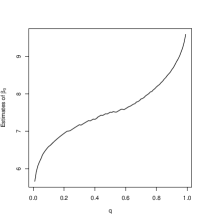
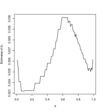
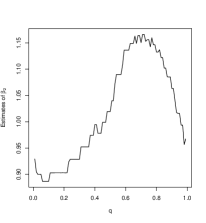
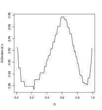
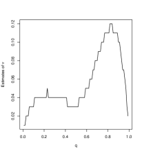
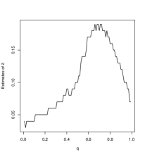
Table 10 presents the ML estimates computed by the EM algorithm and SEs of the CN-BS quantile regression model parameters considering the quantiles $q=0.025,0.25,0.5,0.75,0.975$. For the quantiles analyzed, we can observe that the impact of operational time and legal representation is greater for the quantile $q=0.75$, the same is true with the estimates of ${\alpha}$ and ${\beta}_{0}$.

Table 10: ML estimates (with SE in parentheses) for the CN-BS quantile regression model for the personal accident insurance data.

$q$	Estimate (SE)
	$\widehat{\beta}_{0}$	$\widehat{\beta}_{1}$	$\widehat{\beta}_{2}$	$\widehat{\alpha}$	$\widehat{\nu}$	$\widehat{\delta}$
0.025	5.9965(0.0541)	0.0253(0.0033)	0.9045(0.0630)	0.9138(0.0205)	0.01	0.03
0.25	7.0447(0.0543)	0.0239(0.0033)	0.9286(0.0638)	0.8704(0.0217)	0.04	0.06
0.5	7.5092(0.0543)	0.0272(0.0033)	1.0195(0.0671)	0.9356(0.0220)	0.03	0.10
0.75	8.0053(0.0614)	0.0287(0.0030)	1.1561(0.0694)	0.9281(0.0217)	0.10	0.18
0.975	9.3056(0.0698)	0.0254(0.0033)	0.9936(0.0658)	0.8885(0.0220)	0.05	0.09

Table 11 presents the results for the CN-BS quantile regression model to test the null hypotheses $H_{0}:\beta_{1}=0$ and $H_{0}:\beta_{2}=0$ using the $S_{W}$, $S_{LR}$, $S_{R}$ and $S_{T}$ test statistics. At a 5% significance level, we reject the null hypothesis in all cases tested in Table 11, indicating that coefficients associated with the operating time and legal representation are significant. In addition, from Table 11, we observe that the values of $S_{W}$, $S_{LR}$, $S_{R}$ and $S_{T}$ statistics increase as $q$ increases.

Table 11: Observed values of the indicated test statistics and their $p$-values (in parentheses) for the CN-BS quantile regression model for the personal accident insurance data.

$q$		Test statistics
	Hypothesis	$S_{W}$	$S_{LR}$	$S_{R}$	$S_{T}$
0.25	$H_{0}:\beta_{1}=0$	53.471($<0.0001$)	61.971($<0.0001$)	149.8($<0.0001$)	144.23($<0.0001$)
	$H_{0}:\beta_{2}=0$	212.12($<0.0001$)	13.438(0.0002)	36.392($<0.0001$)	40.174($<0.0001$)
0.5	$H_{0}:\beta_{1}=0$	68.507($<0.0001$)	159.35($<0.0001$)	202.04($<0.0001$)	165.38($<0.0001$)
	$H_{0}:\beta_{2}=0$	230.97($<0.0001$)	17.197($<0.0001$)	42.467($<0.0001$)	47.923($<0.0001$)
0.75	$H_{0}:\beta_{1}=0$	90.682($<0.0001$)	231.28($<0.0001$)	262.37($<0.0001$)	190.9($<0.0001$)
	$H_{0}:\beta_{2}=0$	275.56($<0.0001$)	36.009($<0.0001$)	40.564($<0.0001$)	51.648($<0.0001$)

Figure 5 presents the scatterplot of the amount against the optime according to the group with legal representation and without legal representation with 95% confidence bands in the CN-BS quantile regression model for the personal accident insurance data. We use ML estimates based on the quantiles 2.5% and 97.5% to build these confidence bands. We can see that the upper bound of the confidence bands increases exponentially.

(a) legrep = Yes

(b) legrep = No

Figure 5: 95% confidence bands in the CN-BS quantile regression model for the personal accident insurance data.

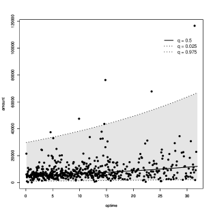
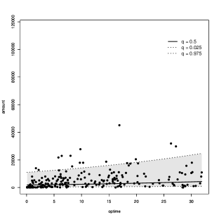
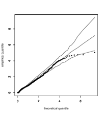
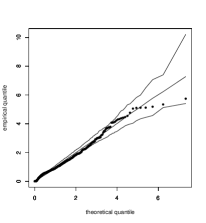
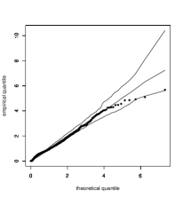
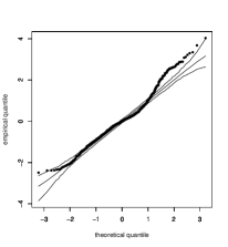
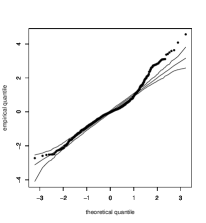
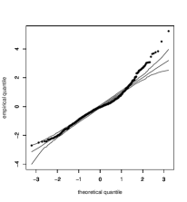
Figure 6 shows the QQ plots with simulated envelope of the GCS and RQ residuals for the CN-BS quantile regression model considered in Table 10. We can see clearly that the CN-BS model provides a good fit based on the GCS residual. On the other hand, the plots for the RQ residuals present some more extreme points outside the region delimited by the confidence bands.

(a) $q=0.25$

(b) $q=0.5$

(c) $q=0.75$

(d) $q=0.25$

(e) $q=0.5$

(f) $q=0.75$

Figure 6: QQ plots and their envelopes for the GCS ((a), (b) and (c)) and RQ ((d), (e) and (f)) residuals in the CN-BS quantile regression model for the personal accident insurance data.

6 Concluding remarks

In this paper, we have proposed a class of quantile regression models based on the reparameterized scale-mixture Birnbaum-Saunders distributions, which have the distribution quantile as one of their parameters. The relevance of this work lies in the proposal of a new quantile regression model that presents a new alternative capable of providing a very flexible fit for strictly positive and asymmetric data. The results obtained in the Monte Carlo simulation studies showed that (a) the maximum likelihood estimates obtained by the EM algorithm, in terms of bias, MSE and CP, perform well; (b) the GCS and RQ residuals conform well with their respective reference distributions with the exception of the SL-BS model; and (c) the Wald, likelihood ratio, score and gradient tests have similar performances. However, in terms of power, the Wald and gradient tests have null rejection rates closer to their nominal levels. Thus, the Wald and gradient tests are preferable to the other tests analyzed. We have applied the proposed models to a real data set related to personal accident insurance. The application results showed the flexibility of the proposed model by providing a richer characterization of the effects of the covariates on the dependent variable. As part of future research, it will be of interest to study influence diagnostic tools as well as multivariate versions. Furthermore, Bartlett and Bartlett-type corrections can be used to attenuate the size distortion of hypothesis tests. Work on these problems is currently in progress and we hope to report these findings in future papers.

Acknowledgements

Helton Saulo and Roberto Vila gratefully acknowledges financial support from CNPq, CAPES, and FAP-DF, Brazil.

Disclosure statement

There are no conflicts of interest to disclose.

Appendix A Simulation results: Hypothesis tests

Table 12: Null rejection rates for $H_{0}:\beta_{1}=\beta_{2}=\beta_{3}=0$ in the CN-BS quantile regression model ($\nu=0.1$, $\delta=0.3$).

$n=50$ $n=100$ $n=200$ $\alpha$ $q$ 1% 5% 10% 1% 5% 10% 1% 5% 10% 0.2 0.25 $S_{W}$ 0.0156 0.057 0.1082 0.0124 0.054 0.1046 0.0108 0.0512 0.1028 $S_{LR}$ 0.021 0.0792 0.1402 0.0202 0.0778 0.1344 0.0188 0.0742 0.1362 $S_{R}$ 0.0388 0.1204 0.1972 0.0232 0.0836 0.1488 0.015 0.0662 0.1214 $S_{T}$ 0.0066 0.0476 0.1024 0.0102 0.0472 0.0978 0.009 0.0468 0.1012 0.5 $S_{W}$ 0.019 0.0608 0.1078 0.0158 0.0558 0.1034 0.011 0.0478 0.0956 $S_{LR}$ 0.02 0.085 0.1402 0.0146 0.0726 0.129 0.0142 0.0666 0.122 $S_{R}$ 0.0294 0.1032 0.1704 0.0188 0.0706 0.1266 0.014 0.0646 0.1284 $S_{T}$ 0.0066 0.0446 0.0944 0.0094 0.0458 0.0958 0.0084 0.046 0.1 0.75 $S_{W}$ 0.0184 0.0614 0.1066 0.0128 0.0536 0.1046 0.0142 0.0504 0.0998 $S_{LR}$ 0.0212 0.0764 0.1332 0.0166 0.07 0.132 0.0172 0.0728 0.139 $S_{R}$ 0.0496 0.1384 0.2166 0.0284 0.1004 0.1636 0.019 0.061 0.1178 $S_{T}$ 0.0074 0.0436 0.1002 0.0106 0.045 0.101 0.0092 0.047 0.1008 0.5 0.25 $S_{W}$ 0.017 0.0544 0.099 0.0124 0.051 0.0994 0.0094 0.0492 0.1022 $S_{LR}$ 0.0192 0.0798 0.141 0.0166 0.0662 0.1226 0.0142 0.071 0.123 $S_{R}$ 0.0664 0.1646 0.245 0.0228 0.0814 0.143 0.0134 0.0596 0.116 $S_{T}$ 0.0074 0.0464 0.098 0.0102 0.0474 0.0978 0.0086 0.047 0.1002 0.5 $S_{W}$ 0.0128 0.0568 0.1044 0.0114 0.0536 0.1014 0.0104 0.0514 0.1002 $S_{LR}$ 0.025 0.0832 0.1364 0.0166 0.0656 0.1252 0.0144 0.0638 0.1182 $S_{R}$ 0.0266 0.0994 0.1678 0.0176 0.0668 0.1266 0.0138 0.0638 0.1202 $S_{T}$ 0.0068 0.0446 0.0944 0.0094 0.0458 0.0956 0.0084 0.0458 0.0996 0.75 $S_{W}$ 0.0154 0.0636 0.1052 0.0136 0.0532 0.1004 0.0118 0.053 0.0996 $S_{LR}$ 0.0166 0.0746 0.1338 0.0154 0.0782 0.135 0.0166 0.0728 0.13 $S_{R}$ 0.0406 0.1244 0.1922 0.0258 0.0834 0.141 0.013 0.0594 0.1104 $S_{T}$ 0.0076 0.043 0.1008 0.0108 0.0444 0.0992 0.0088 0.0468 0.1012 1 0.25 $S_{W}$ 0.0128 0.0452 0.0866 0.0108 0.046 0.0862 0.0084 0.0448 0.0954 $S_{LR}$ 0.017 0.071 0.1252 0.015 0.0642 0.116 0.0146 0.0632 0.1136 $S_{R}$ 0.07 0.1586 0.241 0.0224 0.0798 0.1482 0.0142 0.0668 0.1256 $S_{T}$ 0.0074 0.046 0.0988 0.0104 0.0472 0.098 0.0088 0.0462 0.1016 0.5 $S_{W}$ 0.0122 0.0478 0.0908 0.013 0.047 0.0938 0.0104 0.0488 0.0944 $S_{LR}$ 0.0206 0.0772 0.1318 0.0138 0.0622 0.122 0.0144 0.0578 0.1072 $S_{R}$ 0.0292 0.1054 0.174 0.0186 0.0718 0.1276 0.014 0.0644 0.1208 $S_{T}$ 0.0068 0.0444 0.0948 0.0094 0.0462 0.0962 0.0084 0.0454 0.1004 0.75 $S_{W}$ 0.0194 0.0534 0.0922 0.0106 0.0486 0.0888 0.0092 0.0514 0.101 $S_{LR}$ 0.0208 0.0726 0.1276 0.0138 0.0622 0.115 0.0158 0.0642 0.113 $S_{R}$ 0.0454 0.1348 0.207 0.0208 0.0866 0.1506 0.0126 0.0592 0.1128 $S_{T}$ 0.0078 0.043 0.1012 0.011 0.0462 0.1022 0.0086 0.0464 0.1014

Table 13: Null rejection rates for $H_{0}:\beta_{1}=\beta_{2}=\beta_{3}=0$ in the SL-BS quantile regression model ($\nu=4$).

$n=50$ $n=100$ $n=200$ $\alpha$ $q$ 1% 5% 10% 1% 5% 10% 1% 5% 10% 0.2 0.25 $S_{W}$ 0.0146 0.0584 0.1 0.0118 0.0506 0.0974 0.0096 0.0468 0.0956 $S_{LR}$ 0.016 0.0658 0.125 0.013 0.0616 0.117 0.0126 0.0542 0.1038 $S_{R}$ 0.0446 0.1258 0.2072 0.0222 0.0892 0.152 0.017 0.0702 0.1286 $S_{T}$ 0.0072 0.0436 0.0916 0.0078 0.0436 0.096 0.009 0.0524 0.101 0.5 $S_{W}$ 0.0148 0.0496 0.0902 0.0118 0.0506 0.0974 0.0096 0.0468 0.0954 $S_{LR}$ 0.0154 0.0666 0.1284 0.0164 0.0632 0.119 0.0118 0.0548 0.1092 $S_{R}$ 0.0664 0.1626 0.2434 0.0188 0.0736 0.1406 0.0148 0.0664 0.1254 $S_{T}$ 0.0066 0.0426 0.0914 0.0082 0.0494 0.1004 0.0108 0.045 0.0948 0.75 $S_{W}$ 0.015 0.0496 0.0902 0.0118 0.0508 0.0974 0.0096 0.0468 0.0952 $S_{LR}$ 0.015 0.0676 0.1236 0.0118 0.0574 0.1106 0.0104 0.0572 0.1054 $S_{R}$ 0.0422 0.124 0.1978 0.026 0.0882 0.1554 0.0176 0.064 0.1146 $S_{T}$ 0.007 0.0474 0.1028 0.0062 0.0458 0.0926 0.0086 0.0482 0.096 0.5 0.25 $S_{W}$ 0.0136 0.0446 0.0826 0.0114 0.047 0.0916 0.0096 0.0454 0.0904 $S_{LR}$ 0.016 0.0708 0.129 0.0152 0.0544 0.1066 0.0102 0.05 0.1042 $S_{R}$ 0.0418 0.1262 0.2064 0.027 0.089 0.1538 0.0158 0.0684 0.1182 $S_{T}$ 0.0058 0.0424 0.095 0.0078 0.0488 0.0974 0.0094 0.0486 0.1 0.5 $S_{W}$ 0.0136 0.0446 0.0826 0.0114 0.047 0.0916 0.0096 0.0454 0.0902 $S_{LR}$ 0.0144 0.0666 0.121 0.0134 0.0584 0.109 0.013 0.0566 0.1048 $S_{R}$ 0.0436 0.1268 0.2104 0.0332 0.1036 0.169 0.013 0.0602 0.1174 $S_{T}$ 0.0042 0.0438 0.0994 0.0104 0.0456 0.0928 0.0112 0.0476 0.1008 0.75 $S_{W}$ 0.0136 0.0446 0.0824 0.0114 0.047 0.0916 0.0096 0.0454 0.0902 $S_{LR}$ 0.0156 0.0608 0.1194 0.0124 0.0574 0.1072 0.012 0.0566 0.1064 $S_{R}$ 0.0366 0.1098 0.1852 0.026 0.0896 0.156 0.0178 0.0694 0.1288 $S_{T}$ 0.0062 0.046 0.0984 0.007 0.0408 0.0944 0.0094 0.0562 0.103 1 0.25 $S_{W}$ 0.0088 0.031 0.0608 0.0102 0.0366 0.0738 0.0088 0.0394 0.0834 $S_{LR}$ 0.013 0.0618 0.113 0.009 0.0504 0.0992 0.01 0.045 0.0946 $S_{R}$ 0.045 0.1288 0.21 0.027 0.0942 0.1568 0.0122 0.0638 0.1268 $S_{T}$ 0.008 0.0478 0.0928 0.008 0.0508 0.1056 0.0112 0.0486 0.0966 0.5 $S_{W}$ 0.0088 0.0308 0.0608 0.0102 0.0366 0.0738 0.0088 0.0394 0.0834 $S_{LR}$ 0.013 0.0578 0.112 0.0114 0.05 0.0992 0.0084 0.0428 0.0934 $S_{R}$ 0.0338 0.108 0.183 0.0206 0.0762 0.1396 0.0114 0.0602 0.1142 $S_{T}$ 0.0064 0.046 0.0974 0.0076 0.047 0.0974 0.0088 0.0502 0.104 0.75 $S_{W}$ 0.0088 0.0308 0.0608 0.0102 0.0366 0.0738 0.0088 0.0394 0.0834 $S_{LR}$ 0.0144 0.0594 0.1148 0.0084 0.0468 0.0894 0.0094 0.0528 0.0978 $S_{R}$ 0.0586 0.1494 0.231 0.0216 0.0826 0.1496 0.0128 0.0644 0.1218 $S_{T}$ 0.0054 0.0436 0.0916 0.0088 0.0468 0.0934 0.0086 0.0498 0.0994

Table 14: Null rejection rates for $H_{0}:\beta_{1}=\beta_{2}=\beta_{3}=0$ in the $t_{\nu}$-BS quantile regression model ($\nu=11$).

$n=50$ $n=100$ $n=200$ $\alpha$ $q$ 1% 5% 10% 1% 5% 10% 1% 5% 10% 0.2 0.25 $S_{W}$ 0.016 0.063 0.1128 0.0112 0.0522 0.0982 0.0104 0.0494 0.0984 $S_{LR}$ 0.0178 0.0712 0.1304 0.0156 0.0668 0.1214 0.0138 0.0604 0.1164 $S_{R}$ 0.0452 0.1308 0.2092 0.0154 0.0704 0.129 0.015 0.0692 0.1254 $S_{T}$ 0.0086 0.0498 0.1016 0.0068 0.043 0.0918 0.0082 0.0478 0.0962 0.5 $S_{W}$ 0.0156 0.0662 0.1232 0.016 0.0566 0.1074 0.012 0.0538 0.106 $S_{LR}$ 0.0192 0.079 0.1418 0.0146 0.066 0.124 0.013 0.058 0.1102 $S_{R}$ 0.0422 0.1188 0.1908 0.015 0.0662 0.123 0.0122 0.0568 0.1126 $S_{T}$ 0.0058 0.0394 0.0886 0.0094 0.0454 0.0934 0.0096 0.0506 0.102 0.75 $S_{W}$ 0.0214 0.0674 0.1206 0.0138 0.0572 0.1084 0.0116 0.058 0.1032 $S_{LR}$ 0.018 0.0676 0.1364 0.0146 0.0594 0.1156 0.0138 0.063 0.1176 $S_{R}$ 0.0604 0.1486 0.2198 0.0168 0.0668 0.127 0.0156 0.0618 0.1204 $S_{T}$ 0.0092 0.0522 0.1064 0.0086 0.0486 0.0982 0.0092 0.0452 0.095 0.5 0.25 $S_{W}$ 0.0144 0.0612 0.111 0.0112 0.0492 0.0958 0.011 0.0554 0.1026 $S_{LR}$ 0.015 0.0678 0.131 0.0164 0.0674 0.122 0.0112 0.0576 0.1062 $S_{R}$ 0.0432 0.1368 0.208 0.0194 0.0806 0.1418 0.0164 0.0668 0.1248 $S_{T}$ 0.0086 0.0502 0.1046 0.0068 0.0438 0.0916 0.008 0.0454 0.0922 0.5 $S_{W}$ 0.0188 0.0614 0.1116 0.0128 0.0544 0.097 0.0106 0.0518 0.0996 $S_{LR}$ 0.0156 0.0694 0.1284 0.014 0.0586 0.1118 0.0108 0.0626 0.1174 $S_{R}$ 0.041 0.1124 0.1846 0.021 0.0758 0.143 0.0124 0.0608 0.1186 $S_{T}$ 0.006 0.0456 0.0988 0.0094 0.05 0.1024 0.0066 0.0452 0.0948 0.75 $S_{W}$ 0.0172 0.0548 0.1032 0.01 0.0566 0.1038 0.0108 0.0494 0.0972 $S_{LR}$ 0.0144 0.072 0.1354 0.0142 0.059 0.1112 0.0126 0.0624 0.1218 $S_{R}$ 0.0474 0.1302 0.2032 0.018 0.0736 0.1328 0.0138 0.0624 0.1186 $S_{T}$ 0.0084 0.0496 0.1016 0.0086 0.0436 0.0912 0.0084 0.049 0.0946 1 0.25 $S_{W}$ 0.0118 0.0478 0.0898 0.0118 0.042 0.0864 0.0106 0.0446 0.0874 $S_{LR}$ 0.0138 0.0604 0.1128 0.0134 0.058 0.1058 0.0138 0.055 0.1016 $S_{R}$ 0.0544 0.1374 0.2124 0.0156 0.0708 0.1356 0.0144 0.0638 0.1252 $S_{T}$ 0.0086 0.0514 0.105 0.0068 0.044 0.0916 0.0098 0.0544 0.1016 0.5 $S_{W}$ 0.0102 0.043 0.0848 0.0102 0.048 0.094 0.01 0.0452 0.0936 $S_{LR}$ 0.016 0.0664 0.1232 0.0136 0.0552 0.1074 0.0116 0.0498 0.097 $S_{R}$ 0.0196 0.0844 0.1572 0.0122 0.0698 0.137 0.0134 0.0592 0.1218 $S_{T}$ 0.008 0.0452 0.0998 0.0086 0.0508 0.0974 0.009 0.0472 0.096 0.75 $S_{W}$ 0.0144 0.0484 0.0882 0.0094 0.0464 0.094 0.011 0.0482 0.0974 $S_{LR}$ 0.0178 0.0696 0.1236 0.0096 0.0526 0.1 0.0122 0.0528 0.1074 $S_{R}$ 0.0416 0.1196 0.1964 0.0224 0.082 0.1416 0.0114 0.0592 0.1132 $S_{T}$ 0.0072 0.049 0.0982 0.0082 0.0518 0.1028 0.011 0.051 0.099

References

- Andrews and Mallows, (1974) Andrews, D. F. and Mallows, C. L. (1974). Scale mixtures of normal distributions. Journal of the Royal Statistical Society: Series B (Methodological), 36(1):99–102.
- Baker, (1992) Baker, S. G. (1992). A simple method for computing the observed information matrix when using the em algorithm with categorical data. Journal of Computational and Graphical Statistics, 1(1):63–76.
- Balakrishnan and Kundu, (2019) Balakrishnan, N. and Kundu, D. (2019). Birnbaum-saunders distribution: A review of models, analysis, and applications. Applied Stochastic Models in Business and Industry, 35:4–49.
- Balakrishnan et al., (2009) Balakrishnan, N., Leiva, V., Sanhueza, A., Vilca, F., et al. (2009). Estimation in the birnbaum-saunders distribution based on scale-mixture of normals and the em-algorithm. SORT-Statistics and Operations Research Transactions.
- Cox and Snell, (1968) Cox, D. R. and Snell, E. (1968). A general definition of residuals. Journal of the Royal Statistical Society B, 2:248–275.
- Dasilva et al., (2020) Dasilva, A., Dias, R., Leiva, V., Marchant, C., and Saulo, H. (2020). [Invited tutorial] Birnbaum-Saunders regression models: a comparative evaluation of three approaches. Journal of Statistical Computation and Simulation, pages 1–19.
- De Jong et al., (2008) De Jong, P., Heller, G. Z., et al. (2008). Generalized linear models for insurance data. Cambridge Books.
- Dempster et al., (1977) Dempster, A. P., Laird, N. M., and Rubin, D. B. (1977). Maximum likelihood from incomplete data via the em algorithm. Journal of the Royal Statistical Society: Series B (Methodological), 39(1):1–22.
- Dunn and Smyth, (1996) Dunn, P. and Smyth, G. (1996). Randomized quantile residuals. Journal of Computational and Graphical Statistics, 5:236–244.
- Efron and Olshen, (1978) Efron, B. and Olshen, R. A. (1978). How broad is the class of normal scale mixtures? The Annals of Statistics, pages 1159–1164.
- Fernández and Steel, (1999) Fernández, C. and Steel, M. F. (1999). Multivariate student-t regression models: Pitfalls and inference. Biometrika, 86(1):153–167.
- Gneiting, (1997) Gneiting, T. (1997). Normal scale mixtures and dual probability densities. Journal of Statistical Computation and Simulation, 59(4):375–384.
- Huang and Qu, (2006) Huang, S. and Qu, Y. (2006). The loss in power when the test of differential expression is performed under a wrong scale. Journal of Computational Biology, 13:786–797.
- Jamshidian and Jennrich, (1997) Jamshidian, M. and Jennrich, R. I. (1997). Acceleration of the em algorithm by using quasi-newton methods. Journal of the Royal Statistical Society. Series B (Methodological), 59(3):569–587.
- Koenker, (2004) Koenker, R. (2004). Quantile regression for longitudinal data. Journal of Multivariate Analysis, 91(1):74–89.
- Koenker and Bassett Jr, (1978) Koenker, R. and Bassett Jr, G. (1978). Regression quantiles. Econometrica: journal of the Econometric Society, pages 33–50.
- Koenker and Hallock, (2001) Koenker, R. and Hallock, K. F. (2001). Quantile regression. Journal of economic perspectives, 15(4):143–156.
- Lachos et al., (2017) Lachos, V. H., Dey, D. K., Cancho, V. G., and Louzada, F. (2017). Scale mixtures log-birnbaum–saunders regression models with censored data: a bayesian approach. Journal of Statistical Computation and Simulation, 87(10):2002–2022.
- Lachos and Labra, (2007) Lachos, V. H. and Labra, F. (2007). Skew-normal/independent distributions, with applications. Universidade Estadual de Campinas. Instituto de Matemática, Estatística e ….
- Lange and Sinsheimer, (1993) Lange, K. and Sinsheimer, J. S. (1993). Normal/independent distributions and their applications in robust regression. Journal of Computational and Graphical Statistics, 2(2):175–198.
- Lange et al., (1989) Lange, K. L., Little, R. J., and Taylor, J. M. (1989). Robust statistical modeling using the t distribution. Journal of the American Statistical Association, 84(408):881–896.
- Lee and Wang, (2003) Lee, E. T. and Wang, J. (2003). Statistical methods for survival data analysis, volume 476. John Wiley & Sons.
- Leiva, (2016) Leiva, V. (2016). The Birnbaum-Saunders Distribution. Academic Press, New York, US.
- Louis, (1982) Louis, T. A. (1982). Finding the observed information matrix when using the em algorithm. Journal of the Royal Statistical Society: Series B (Methodological), 44(2):226–233.
- Lucas, (1997) Lucas, A. (1997). Robustness of the student t based m-estimator. Communications in Statistics-Theory and Methods, 26(5):1165–1182.
- McLachlan and Krishnan, (2007) McLachlan, G. J. and Krishnan, T. (2007). The EM algorithm and extensions, volume 382. John Wiley & Sons.
- Meilijson, (1989) Meilijson, I. (1989). A fast improvement to the em algorithm on its own terms. Journal of the Royal Statistical Society: Series B (Methodological), 51(1):127–138.
- Naderi et al., (2020) Naderi, M., Hashemi, F., Bekker, A., and Jamalizadeh, A. (2020). Modeling right-skewed financial data streams: A likelihood inference based on the generalized Birnbaum-Saunders mixture model. Applied Mathematics and Computation, 376:125109.
- Oakes, (1999) Oakes, D. (1999). Direct calculation of the information matrix via the em. Journal of the Royal Statistical Society: Series B (Statistical Methodology), 61(2):479–482.
- Paula et al., (2012) Paula, G. A., Leiva, V., Barros, M., and Liu, S. (2012). Robust statistical modeling using the birnbaum-saunders-t distribution applied to insurance. Applied Stochastic Models in Business and Industry, 28(1):16–34.
- R Core Team, (2020) R Core Team (2020). R: A Language and Environment for Statistical Computing. R Foundation for Statistical Computing, Vienna, Austria.
- Rieck and Nedelman, (1991) Rieck, J. R. and Nedelman, J. R. (1991). A log-linear model for the birnbaum—saunders distribution. Technometrics, 33(1):51–60.
- Sánchez et al., (2020) Sánchez, L., Leiva, V., Galea, M., and Saulo, H. (2020). Birnbaum-Saunders quantile regression and its diagnostics with application to economic data. Applied Stochastic Models in Business and Industry, 37:53–73.
- Saulo et al., (2022) Saulo, H., Dasilva, A., Leiva, V., Sánchez, L., and Fuente-Mella, H. L. (2022). Log-symmetric quantile regression models. Statistica Neerlandica, 76:124–163.
- Saulo et al., (2019) Saulo, H., Leão, J., Leiva, V., and Aykroyd, R. G. (2019). Birnbaum-Saunders autoregressive conditional duration models applied to high-frequency financial data. Statistical Papers, 60:1605–1629.
- Saulo et al., (2021) Saulo, H., Leão, J., Nobre, L., and Balakrishnan, N. (2021). A class of asymmetric regression models for left-censored data. Brazilian Journal of Probability and Statistics, 35:62–84.
- Taylor and Verbyla, (2004) Taylor, J. and Verbyla, A. (2004). Joint modelling of location and scale parameters of the t distribution. Statistical Modelling, 4(2):91–112.
- Terrell, (2002) Terrell, G. R. (2002). The gradient statistic. Computing Science and Statistics, 34(34):206–215.
- Walker and Gutiérrez-Peña, (2007) Walker, S. G. and Gutiérrez-Peña, E. (2007). Bayesian parametric inference in a nonparametric framework. Test, 16(1):188–197.
- West, (1987) West, M. (1987). On scale mixtures of normal distributions. Biometrika, 74(3):646–648.
- Yu and Moyeed, (2001) Yu, K. and Moyeed, R. A. (2001). Bayesian quantile regression. Statistics & Probability Letters, 54(4):437–447.