Also at ]John A. Paulson School of Engineering and Applied Sciences, Harvard University
Port-Hamiltonian Neural Networks
for Learning Explicit Time-Dependent Dynamical Systems
Abstract
Accurately learning the temporal behavior of dynamical systems requires models with well-chosen learning biases. Recent innovations embed the Hamiltonian and Lagrangian formalisms into neural networks and demonstrate a significant improvement over other approaches in predicting trajectories of physical systems. These methods generally tackle autonomous systems that depend implicitly on time or systems for which a control signal is known apriori. Despite this success, many real world dynamical systems are non-autonomous, driven by time-dependent forces and experience energy dissipation. In this study, we address the challenge of learning from such non-autonomous systems by embedding the port-Hamiltonian formalism into neural networks, a versatile framework that can capture energy dissipation and time-dependent control forces. We show that the proposed port-Hamiltonian neural network can efficiently learn the dynamics of nonlinear physical systems of practical interest and accurately recover the underlying stationary Hamiltonian, time-dependent force, and dissipative coefficient. A promising outcome of our network is its ability to learn and predict chaotic systems such as the Duffing equation, for which the trajectories are typically hard to learn.
I Introduction
Neural networks (NNs), as universal function approximators [1], have shown resounding success across a host of domains including image segmentation [2], machine translation [3], and material property predictions [4, 5]. However, their performance in learning and generalizing the long-term behaviour of dynamic systems governed by known physical laws from state data has often been limited [6, 7]. New research in scientific machine learning, a field that tackles scientific problems with domain-specific machine learning methods, is paving a way to address this challenge. Concretely, it has been shown that physically-informed learning biases embedded in networks, such as Hamiltonian mechanics [8, 6], Lagrangians [9, 10], Ordinary Differential Equations (ODEs) [11], physics-informed networks [12, 13], generative networks [14], and Graph Neural Networks [15, 16] can significantly improve learning and generalization over vanilla neural networks in complex physical domains. The performance uplift arises primarily because learning biases are able to constrain networks to learn physically meaningful representations from data that are crucial to generalization.
Despite extensive research on learning biases, there is yet no method that accounts for non-autonomous systems i.e. systems with explicit time dependence. Non-autonomous dynamics feature prominently in settings with externally driven or controlled time-dependent forces as well as in systems with energy dissipation, for example, interacting materials, forced oscillators and charge-discharge cycles. Defining a network to accurately learn and predict the dynamics of such systems from position and momentum data is therefore of critical practical interest. We address this challenge by embedding the port-Hamiltonian formalism [17, 18, 19, 20, 21] into neural networks. We show that the structure of this formulation can be used to uncover the underlying Hamiltonian, force and damping terms given position and momentum data and as such, can be used to accurately predict the long-range trajectories of many forced/damped systems. We extensively benchmark our network on a range of tasks including a simple mass-spring system with damping and external force, a Duffing system in both the non-chaotic and chaotic regimes, and a relativistic Duffing system. Our proposed network consistently outperforms other approaches while accurately recovering both the driving force and the damping coefficient. Furthermore, using minimal data, we show that our network can visually recover the Poincaré section of the Duffing system in a chaotic regime, emphasizing how our network can be used to identify and understand chaotic trajectories.
II Background
II.1 Hamiltonian Neural Networks
Recently, the authors of [6] demonstrated that the dynamics of an energy conserving autonomous system can be accurately learned by guiding a neural network to predict a Hamiltonian - an important representation of a dynamical system. Considering a dynamical system of objects, the Hamiltonian is a scalar function of a position vector and momentum vector that obeys Hamilton’s equations,
| (1) |
where and .
Using the Hamiltonian formalism, [6] showed that a NN with parameters can be used to learn a Hamiltonian given and as inputs to the network. The time derivatives are recovered from Eq. (1) by differentiating with respect to its inputs using automatic differentiation. The resulting system has the form,
| (2) |
where and is determined by Eq. (1) after differentiating the trained NN. Eq. (2) can be discretized using a time-integrator to determine the trajectory of an initial state. Moreover, since is the symplectic gradient of the Hamiltonian, energy conservation is embedded into the method by construction. Given these advantages, Hamiltonian Neural Networks (HNNs) outperform traditional approaches that directly predict the state time derivatives from the input state. However, this formulation does not readily generalize to damped or forced time-varying systems.
II.2 Port-Hamiltonian framework
The port-Hamiltonian [17, 18, 19, 20, 21] is a well studied formalism that generalizes Hamilton’s equations to incorporate energy dissipation and an external control input to a dynamical system. Hamilton’s equations in the port-Hamiltonian framework are represented as:
| (3) |
where is a damping matrix, is a temporal control input, is a non-linear scaling of the position vector, is the identity matrix, and the zero matrix. The damping matrix is semi-positive definite. This general formalism readily reduces to the standard Hamiltonian system when and . The port Hamiltonian has been used in control applications where explicit knowledge of the control term is known and was recently shown to reveal promising results in NNs [22]. Note that in [22], the vector is provided as input to the network. However, in many applications the control force is unknown and it is therefore of interest to uncover the underlying forcing term from the data of the state vector, where no explicit knowledge of the control input and damping term is available.
II.3 Related Work
While Hamiltonian mechanics presents one way to address learning dynamical systems, numerous recent methods highlight how incorporating other physically-informed inductive biases into neural networks can improve learning.
Functional priors, for example, embed the full functional form of an equation into the NN. Physics-informed neural networks (PINNs) [12, 23] and Hamiltonian networks [8] are two such approaches that look at directly embedding the equations of motion into the loss function. While PINNs are data-driven approaches that rely on Autograd [24] to compute partial-derivatives of a hidden state, Hamiltonian networks are data-independent approaches that pre-specify the full functional form of a system-specific Hamiltonian in the loss function.
Many recent methods have also sought to embed integrators into the training process. Indeed doing so induces an effectively continuous depth neural network able to perform large time-step predictions. NeuralODE [11] presents one way to tackle back-propagating through this continuous depth network more efficiently.
More recent work has looked at generalizing this approach to different and more complex data structures and topologies that standard NeuralODEs cannot represent [25]. Other work, such as Zhu et al. [26], theoretically shows the importance of using symplectic integrators over Runge-Kutta methods to evolve Hamiltonian systems in NNs.
In [15], the authors detailed how a Graph Neural Network, designed to capture the relational structure of systems, can be used to learn dynamics of interacting particles. This work has been exploited in numerous advances [27, 28, 9] and emphasizes how a relational inductive bias can significantly improve learning.
In [9] and [6] it has been shown that by learning the Hamiltonian or the Lagrangian of a system, it is possible to accurately predict the temporal dynamics and conserve energy. The work of [10] also showed that by exploiting the Euler-Lagrange equation, it is possible to predict a controlled double pendulum - a system pertinent for controlled robots. A recent advance shows that Hamiltonian and Lagrangian NNs can be drastically improved if they are optimized over Cartesian coordinates with holonomic constraints [29].
Despite the significant breakthroughs, there is no existing method that investigates explicit time-dependence and damping in dynamical systems, two elements that are often found in real world problems. As such, we outline a novel technique to address this challenge.
III Method
III.1 Theory
In this section we introduce port-Hamiltonian Neural Networks (pHNNs). We begin by illustrating how a NN takes the form of the port-Hamiltonian formulation of Eq. (3) with two modifications. First, our approach exploits the fact that many damped systems consist of a non-zero, state-independent damping term in the lower right quadrant, so we replace the damping matrix with a state independent matrix for which only the lower right term is non-zero and represented by . Secondly, in order to generalize to time dependent forcing, we replace with the force field . The resulting representation,
|
[˙q˙p] = ([0 I -I 0 ] + [0 0 0 N ] ) [∂H∂q∂H∂p] + [0 F(t) ], |
(4) |
is general enough to handle many well-known forced systems but also specific enough to tackle learning in physical domains of practical importance such as Duffing equation.
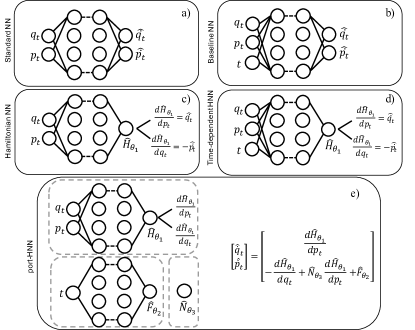
The architecture for the proposed pHNN model and a summary of comparable existing approaches are shown in Fig. 1. A standard feed forward NN in Fig. 1(a) and an HNN in Fig. 1(c) [6] take and as inputs and are trained to yield the time derivatives of the input, with the HNN learning an intermediate Hamiltonian and employing backpropagation to compute the final output. A natural way to extend these architectures for time-varying non-autonomous systems is to include time as an additional input. This gives rise to the baseline network (Baseline NN) represented by Fig. 1(b) and a time-dependent HNN (TDHNN) shown by Fig. 1(d).
Although the Baseline NN and TDHNN incorporate time, they do not provide information for the underlying dynamics of the system. On the other hand, the pHNN is able to extract and provide information about the stationary Hamiltonian, the driving force, and the damping term. Moreover, the pHNN consistently outperforms all the network architectures shown in Figs. 1(a-d) across the applications investigated in this study.
III.2 Network optimization
The training of the pHNN consists of feeding the inputs into the model. The first component, , consists of three hidden layers designed to predict a stationary from input data. The second component, , consists of a single weight parameter (i.e. is a single node) designed to learn the damping. The third neural-network unit solely depends on and consists of three hidden layers designed to predict a time-varying force. The output of each component is transformed through Eq. (4) to obtain predictions of the state time derivatives . Using these predicted quantities we construct the loss function for optimizing the pHNN:
| (5) | ||||
where are known ground truth data. The first two components of the left hand side of Eq. (5) minimize the difference between the predicted and ground truth state time derivatives with a squared error loss. The last two components in Eq. (5) are the forcing and damping terms that are added to the loss function with an penalty when using pHNN. Using an penalty on these terms encourages the network to learn simpler models. We empirically found that this technique prevents the pHNN from learning spurious force and damping terms in unforced and undamped systems compared to an penalty. The regularization parameters and were determined via grid search (see Appendix A). We use 200 nodes per hidden layer and find that most activation functions, including , and yield comparable results.
We generate our data using an RK4 integrator given some initial conditions for each system. We use a small to evaluate the integral and ensure ground truth data is generated with rtol . The gradients of the state at each integration step are computed using the underlying differential equation. Details about the sampling of the initial conditions are described independently for each system in section IV.
We note that in some settings it might be hard to obtain the ground truth state time-derivatives for training. A natural way to address this problem is to embed an integrator into the training, similar to NeuralODE [11]. As such, we also run our study with an embedded RK-4 integrator. Our method is still the most performant when all the methods incorporate an embedded RK-4 integrator (see Appendix) and the loss function is . In other words, our system can learn from either state time derivative data or directly from state data given an embedded integrator. We were motivated to use gradient data since HNN is trained in this way and we wanted a fair comparison.
III.3 Testing
Once trained, each of the networks in Fig. 1 can approximate . As such, these networks can be used in a time integrator to evolve initial conditions in the test set. We refer to the integration for as the state rollout. We measure the performance of the network by comparing the predicted state rollout with the ground truth. Specifically, we assess the networks performance by computing the mean squared error (MSE) of the predicted state variables and predicted energy (Hamiltonian) across the integration time,
| (6) | ||||
| (7) |
where , with the time step size. These terms are computed for multiple initial conditions during inference and averaged across them.
A guide to the training process is outlined in Appendix B.
IV Results
We benchmark the performance of pHNNs against the other networks shown in Fig. 1. We evaluate the methods over datasets that cover simple time-independent systems to complex chaotic damped and driven dynamical systems. The results are presented in order of increasing complexity from a model perspective.
IV.1 Simple Mass-Spring System
We begin our analysis with a simple mass-spring system (harmonic oscillator), obeying Hooke’s Law from classical physics with no force or damping. The Hamiltonian that describes such a system reads:
| (8) |
where is the spring constant and denotes the mass. In this one-dimensional system the position and momentum are scalar functions of time.
Training: Without loss of generalization, we set for our experiments. We randomly sample 25 initial training conditions that satisfy where which corresponds to sampling initial conditions with energies in the range . We evolve each initial state using a RK4 integrator with and .
Testing: We evaluate the performance of the NNs by sampling 25 random initial conditions in the same way as training. We investigate the simple harmonic oscillator system and show that learning a separate, regularized forcing term results in better state and energy predictions in comparison to TDHNN and the Baseline NN. Learning a separate forcing term and regularizing pHNN keeps the time component independent of the Hamiltonian and therefore allows us to closely match the performance of the standard time-implicit HNN.
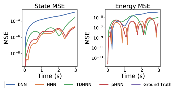
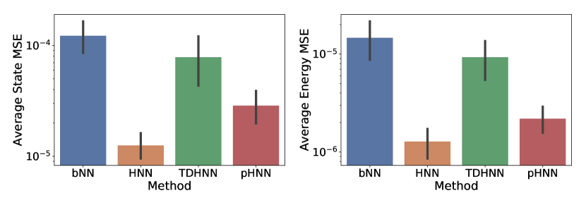
In particular, in Fig. 2(a) we show the state and energy MSE for an initial state from the testing set. Figure 2(b) presents the predicted force (blue solid line) and damping over time (red solid curve), while black dots corresponds to ground truth observations. We observe that the error in the predictions is of the order of for recovering the force function and of for the damping term. In Fig. 2(c) we report the state and energy MSE averaged along all the testing initial states, where the black lines in the histograms represent the error bars of the statistics.

IV.2 Damped Mass-Spring System
We extend the simple mass-spring system to include a damping term that reduces the initial energy of the system over time. The inclusion of this term violates energy conservation and therefore we cannot write a scalar Hamiltonian for such a system (see Appendix C for details). Knowing this a priori already gives us an indication that the HNN will perform poorly on such a system.
Training: We have 20 initial training conditions, with position and momentum uniformly sampled in . Each trajectory is evolved until with a . We fix the damping coefficient without loss of generality.
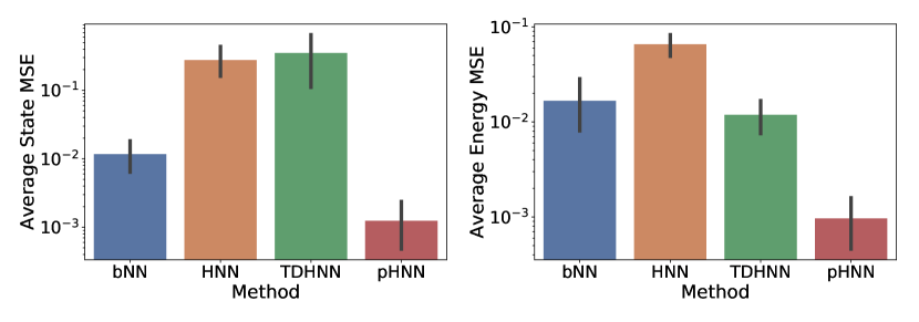
Testing: At inference, we compute the average rollout MSE of 25 unseen initial conditions sampled in the same manner as the training data. Figure 3(a) outlines the predicted force and damping for an arbitrary initial state, while in Fig. 3(b) we report the average state and energy rollout MSE.

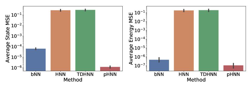
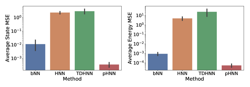
We observe in Fig. 3 that both baseline NN and pHNN recover the dynamics well, whereas th HNN (as expected) and TDHNN struggle to learn the dynamics of the damped system. This failure happens because there is no direct way of writing a scalar Hamiltonian with damping and thus, both the HNN and TDHNN cannot learn the underlying dynamics. This observation indicates that a partial inductive bias is not enough to make a network robust at predicting the dynamics well. A second observation shows that the pHNN learns a non-zero oscillating force. That implies a possible leaking of the information from the predicted Hamiltonian into the predicted force and vice versa. This arises because there is an identifiability challenge inferring the damping and force exclusively from the state data we provide. In spite of this challenge, we find that the pHNN converges to forcing and damping terms consistent with the ground truth generating terms and sufficient to inform us about the underlying dynamics as well as to evolve initial states with small numerical error.
IV.3 Forced Mass-Spring System
We complete the investigation of the simple mass-spring problem by including a driven time-dependent force that controls the system. To understand the effect of the force we consider an undamped driven oscillator system. Typically, while we cannot write the Hamiltonian for a damped system, we can write one for a forced system. We study two cases of forced mass-spring systems. The first has the following Hamiltonian form:
| (9) |
The second has a more complex force described by the Hamiltonian:
| (10) |
where and is the amplitude and frequency of the external force term. The forced mass-spring system is typically used to study resonance effects, e.g. in material science, and plays an important role in a wide range of applications including music, bridge design, and molecular excitation making it an important system to investigate.


Training: In both systems of Hamiltonian Eqs. (9) and (10), we use 20 initial conditions, where the initial state is sampled such that where . For the force term we set and , and without loss of generality we set . The states are rolled out to at a .
Testing: At inference, we compute the rollout of 25 unseen initial conditions in the same range as the training data. Figures 4a and 5a demonstrate the predicted forces and dissipation terms for the systems of Eqs. (9) and (10), respectively. Accordingly, in Figs. 4(b) and 5(b) we report the average state and energy rollout MSE for each system.
We study both systems to illustrate that while the baseline NN performs relatively well in comparison to the pHNN when a simple force is considered such as in the system of Eq. (9), a more complex force significantly hurts its performance in terms of state/energy MSE shown by Fig. 5(b). More importantly, we read in Figs. 4(a) and 5(a) that for both systems pHNN can recover the ground truth force quite precisely while it learns very small spurious damping terms that do not significantly contribute to the dynamics; the contribution to term is of the order , which is practically negligible.
IV.4 Duffing Equation
Another problem that we investigate is given by the Duffing equation, a nonlinear dynamical system that includes both forcing and damping. The unforced and undamped stationary Hamiltonian of the Duffing system is given by:
| (11) |
Unlike the simple mass-spring system, the Duffing equation has an additional quadratic function of that makes the system non-harmonic. The shape of the potential function can be tuned to be a double-well or a single well based on the coefficients and . The general Duffing equation includes a time variant force and a damping term proportional to . Typically the Duffing nonlinear equation of motion is written as:
| (12) |
Different combinations of parameters make the Duffing system either chaotic or non-chaotic. We study both regimes. The Duffing equation reveals numerous phenomena of practical importance including frequency hysteresis (e.g. in magnets), elasticity and chaos theory.


IV.4.1 Non-Chaotic regime
Given a set of initial parameters for the Duffing equation: we can obtain training data in a non-chaotic regime of the Duffing system.
Training: We uniformly sample initial conditions in and use 25 initial conditions for training, rolled out to with .
Testing: We integrate 25 unseen initial conditions at inference using the same and used to generate the training set. We evaluate all the neural network models on this testing set and present the results in Fig. 7. We observe in Fig. 7(a) that pHNN accurately recovers the underlying force and damping. Moreover, Fig. 7(b) indicates the pHNN outperforms the other models used in this study. We further assess the network performance by inspecting the predicted Hamiltonian. In Fig. 9 we outline the learnt as a function of and that comprise the phase space. We observe that pHNN can learn the functional form of , outperforming the other architectures.

IV.4.2 Chaotic regime
The choice of the parameters: , yields chaotic behavior in the Duffing system. Chaotic trajectories are highly sensitive to initial conditions and thus, it is much more difficult to learn from a chaotic system than from a non-chaotic.
Training: 20 initial conditions, sampled uniformly in each rolled out for one period where resulting in 2000 training points.
Testing: We test our system by assessing whether it is visually able to recover the ground truth Poincaré section of an initial condition and we focus our attention on baseline NN and pHNN since they are the most performant in the non-chaotic regime. The Poincaré map (or section) of a trajectory is measured by plotting the position and momentum values at regular intervals governed by the period of the forcing term. For example, a simple mass-spring system will generate a single point in phase space when measured at regular intervals, while a chaotic system generates a more complex map. To visually assess the performance of our network through a Poincaré map, we test the system on a single initial condition, not used in the training set, rolled out to with the same as in the training phase. In order to integrate our system to such a large for this example we work under the assumption that we have explicit knowledge of the period of the force, and as such, we normalize the time variable with the period. We emphasize that while prior knowledge of assists the training, it is only used to extract the Poincaré map. This is necessary as the models are not explicitly trained on time steps beyond . The results are demonstrated in Fig. 6. In our study we find that the visual similarity between the section generated by pHNN is much closer to the ground truth than baseline. A simple quantitative measure of this similarity can be computed using the MSE between the 2D histogram plots. The pHNN results in 1.61 and bNN in 4.05. The outcome suggests that the pHNN can indeed be used to model chaos even after being trained with only a few data points from a chaotic trajectory. We believe this is a valuable result, since it implies that the pHNN can be used to model chaotic behavior.
IV.5 Relativistic System
In the final experiment presented in this study, we go beyond non-relativistic classical mechanics and explore a different form of Hamiltonians. In particular, we investigate the motion of a driven relativistic particle in a nonlinear double well potential, which is mathematically represented by the Duffing equation in a relativistic framework. The Hamiltonian under consideration is:
| (13) |
where is the speed of light that typically is set to 1. For simplicity, we also set the rest mass , though our framework naturally accounts for other values.
Training. We train on 25 initial conditions, uniformly sampled in . We consider , , and the parameters .
Testing. Using the same parameters as training, we roll out 25 unseen initial conditions and present the results in Fig. 8. We observe that pHNN is able to recover the underlying force and outperforms the other architectures in generating the temporal state of previously unknown initial conditions. This experiment is evidence that pHNN can discover the dynamics of temporal systems independent of the form of the underlying Hamiltonian and consistently outperforms the other architectures investigated in this study.
V Discussion
We have shown that pHNN outperforms other approaches in learning complex physical systems (details shown in Appendix D and E), as well as being able to recover the underlying stationary Hamiltonian, the external time varying force, and the damping term of non-autonomous systems. One challenge in achieving this result is fine-tuning the and regularisation coefficients for the force and damping. In the Duffing setting where we have both terms, it is possible to learn a shifted force i.e. . This is possible because the state-vectors do not provide enough information to simultaneously identify both the Hamiltonian and the force resulting in a leak of information between and . Nevertheless, we find that a reasonable force and damping term are generally learnt which are sufficient to reveal the underlying dynamics.
While it may be argued that pHNN is constrained to learn and predict within the training time horizon, we believe our method is still versatile at informing us of periodic forcing, since we can inspect the force over time and, essentially, learn the period of the underlying force. This, in turn, can readily be used to renormalize the time variable at periodic intervals to integrate the system beyond the training time as we showed in the Poincaré map of Fig. 6.
We also run the entire set of experiments on noisy input state vectors where the noise is sampled from with . The details of the results can be found in Appendix F. We find that even with the addition of noise to the input state-vector, pHNN outperforms other methods.
We also carry out a simple study on a 2 body coupled spring system where one of the masses is forced by a cosine varying signal. The results indicate that pHNN performs the best and has potential to scale to larger domains (see Appendix).
VI Conclusion
We have shown that learning the dynamics of time-dependent non-autonomous systems can be achieved with pHNN, a versatile neural network embedded with the Port-Hamiltonian formulation. Our experimental investigation demonstrates that pHNN outperforms extensions of existing methods in numerous settings. Specifically, we outlined that the proposed network not only learns the underlying dynamics of a simple mass-spring system, achieving comparable performance to the efficient HNN architecture, but it extends to more complex nonlinear forced and damped physical systems. Furthermore, using pHNN we were able to show, with minimal training data, the ability to recover the Poincaré section of a chaotic driven system. Unlike existing methods, pHNN is able to identify systems where minimal state data is available and reveal the functional form of the controlling force, damping, and underlying stationary Hamiltonian. Collectively, these results form a strong basis for further advances in learning complex systems including, but not limited to, chemical bond forces, robotic motion, and more general controlled dynamics without explicit knowledge of the force and damping.
References
- Hornik et al. [1989] K. Hornik, M. Stinchcombe, and H. White, Multilayer feedforward networks are universal approximators, Neural Networks 2, 359 (1989).
- He et al. [2018] K. He, G. Gkioxari, P. Dollár, and R. Girshick, Mask R-CNN, arXiv:1703.06870 [cs] (2018), arXiv: 1703.06870.
- Devlin et al. [2019] J. Devlin, M.-W. Chang, K. Lee, and K. Toutanova, BERT: Pre-training of Deep Bidirectional Transformers for Language Understanding, arXiv:1810.04805 [cs] (2019), arXiv: 1810.04805.
- Toussaint et al. [2018] M. Toussaint, K. Allen, K. Smith, and J. Tenenbaum, Differentiable Physics and Stable Modes for Tool-Use and Manipulation Planning, in Robotics: Science and Systems XIV (Robotics: Science and Systems Foundation, 2018).
- Yao et al. [2018] K. Yao, J. E. Herr, D. Toth, R. Mckintyre, and J. Parkhill, The TensorMol-0.1 model chemistry: a neural network augmented with long-range physics, Chemical Science 9, 2261 (2018).
- Greydanus et al. [2019] S. Greydanus, M. Dzamba, and J. Yosinski, Hamiltonian Neural Networks, in Advances in Neural Information Processing Systems 32, edited by H. Wallach, H. Larochelle, A. Beygelzimer, F. d. Alché-Buc, E. Fox, and R. Garnett (Curran Associates, Inc., 2019) pp. 15379–15389.
- Pukrittayakamee et al. [2009] A. Pukrittayakamee, M. Malshe, M. Hagan, L. M. Raff, R. Narulkar, S. Bukkapatnum, and R. Komanduri, Simultaneous fitting of a potential-energy surface and its corresponding force fields using feedforward neural networks, The Journal of Chemical Physics 130, 134101 (2009).
- Mattheakis et al. [2020] M. Mattheakis, D. Sondak, A. S. Dogra, and P. Protopapas, Hamiltonian Neural Networks for solving differential equations, arXiv:2001.11107 [physics] (2020), arXiv: 2001.11107.
- Cranmer et al. [2020] M. Cranmer, S. Greydanus, S. Hoyer, P. Battaglia, D. Spergel, and S. Ho, Lagrangian Neural Networks, arXiv:2003.04630 [physics, stat] (2020), arXiv: 2003.04630.
- Lutter et al. [2019] M. Lutter, C. Ritter, and J. Peters, Deep Lagrangian Networks: Using Physics as Model Prior for Deep Learning, arXiv:1907.04490 [cs, eess, stat] (2019), arXiv: 1907.04490.
- Chen et al. [2018] R. T. Q. Chen, Y. Rubanova, J. Bettencourt, and D. K. Duvenaud, Neural Ordinary Differential Equations, in Advances in Neural Information Processing Systems 31, edited by S. Bengio, H. Wallach, H. Larochelle, K. Grauman, N. Cesa-Bianchi, and R. Garnett (Curran Associates, Inc., 2018) pp. 6571–6583.
- Raissi et al. [2017] M. Raissi, P. Perdikaris, and G. E. Karniadakis, Physics Informed Deep Learning (Part I): Data-driven Solutions of Nonlinear Partial Differential Equations, arXiv:1711.10561 [cs, math, stat] (2017), arXiv: 1711.10561.
- Choudhary et al. [2020] A. Choudhary, J. F. Lindner, E. G. Holliday, S. T. Miller, S. Sinha, and W. L. Ditto, Physics-enhanced neural networks learn order and chaos, Phys. Rev. E 101, 062207 (2020).
- Toth et al. [2020] P. Toth, D. J. Rezende, A. Jaegle, S. Racaniere, A. Botev, and I. Higgins, Hamiltonian generative networks, in International Conference on Learning Representations (2020).
- Battaglia et al. [2016] P. W. Battaglia, R. Pascanu, M. Lai, D. Rezende, and K. Kavukcuoglu, Interaction Networks for Learning about Objects, Relations and Physics, arXiv:1612.00222 [cs] (2016), arXiv: 1612.00222.
- Sanchez-Gonzalez et al. [2019] A. Sanchez-Gonzalez, V. Bapst, K. Cranmer, and P. Battaglia, Hamiltonian Graph Networks with ODE Integrators, arXiv:1909.12790 [physics] (2019), arXiv: 1909.12790.
- van der Schaft [2007] A. van der Schaft, Port-Hamiltonian systems: an introductory survey, in Proceedings of the International Congress of Mathematicians Madrid, August 22–30, 2006, edited by M. Sanz-Solé, J. Soria, J. L. Varona, and J. Verdera (European Mathematical Society Publishing House, Zuerich, Switzerland, 2007) pp. 1339–1365.
- Ortega et al. [2002] R. Ortega, A. van der Schaft, B. Maschke, and G. Escobar, Interconnection and damping assignment passivity-based control of port-controlled hamiltonian systems, Automatica 38, 585 (2002).
- Acosta et al. [2005] J. A. Acosta, R. Ortega, A. Astolfi, and A. D. Mahindrakar, Interconnection and damping assignment passivity-based control of mechanical systems with underactuation degree one, IEEE Transactions on Automatic Control 50, 1936 (2005), conference Name: IEEE Transactions on Automatic Control.
- Zheng et al. [2018] M. Zheng, T. Yuan, and T. Huang, Time-Varying Impedance Control of Port Hamiltonian System with a New Energy-Storing Tank (2018), iSSN: 1076-2787 Pages: e8134230 Publisher: Hindawi Volume: 2018.
- Cherifi [2020] K. Cherifi, An overview on recent machine learning techniques for Port Hamiltonian systems, Physica D: Nonlinear Phenomena 411, 132620 (2020).
- Zhong et al. [2020] Y. D. Zhong, B. Dey, and A. Chakraborty, Dissipative SymODEN: Encoding Hamiltonian Dynamics with Dissipation and Control into Deep Learning, arXiv:2002.08860 [cs, eess, stat] (2020), arXiv: 2002.08860.
- Raissi et al. [2019] M. Raissi, P. Perdikaris, and G. E. Karniadakis, Physics-informed neural networks: A deep learning framework for solving forward and inverse problems involving nonlinear partial differential equations, Journal of Computational Physics 378, 686 (2019).
- [24] D. Maclaurin, D. Duvenaud, and R. P. Adams, Autograd Effortless Gradients in Numpy, , 3.
- Dupont et al. [2019] E. Dupont, A. Doucet, and Y. W. Teh, Augmented Neural ODEs, arXiv:1904.01681 [cs, stat] (2019), arXiv: 1904.01681.
- Zhu et al. [2020] A. Zhu, P. Jin, and Y. Tang, Deep Hamiltonian networks based on symplectic integrators, arXiv:2004.13830 [cs, math] (2020), arXiv: 2004.13830.
- Sanchez-Gonzalez et al. [2018] A. Sanchez-Gonzalez, N. Heess, J. T. Springenberg, J. Merel, M. Riedmiller, R. Hadsell, and P. Battaglia, Graph networks as learnable physics engines for inference and control, arXiv:1806.01242 [cs, stat] (2018), arXiv: 1806.01242.
- Sanchez-Gonzalez et al. [2020] A. Sanchez-Gonzalez, J. Godwin, T. Pfaff, R. Ying, J. Leskovec, and P. W. Battaglia, Learning to Simulate Complex Physics with Graph Networks, arXiv:2002.09405 [physics, stat] (2020), arXiv: 2002.09405.
- Finzi et al. [2020] M. Finzi, S. Stanton, P. Izmailov, and A. G. Wilson, Generalizing Convolutional Neural Networks for Equivariance to Lie Groups on Arbitrary Continuous Data, arXiv:2002.12880 [cs, stat] (2020), arXiv: 2002.12880.