A study on reliability of a kπ‘˜k-out-of-n𝑛n system equipped with a cold standby component based on copula

Achintya Roy, Nitin Gupta Department of Mathematics, Indian Institute of Technology Kharagpur, West Bengal, INDIA.
Email: acroy21@iitkgp.ac.in (Achintya Roy), nitin.gupta@maths.iitkgp.ac.in (Nitin Gupta).
Abstract

A kπ‘˜k-out-of-n𝑛n system consisting of n𝑛n exchangeable components equipped with a single cold standby component is considered. All the components including standby are assumed to be dependent and this dependence is modeled by a copula function. An exact expression for the reliability function of the considered system has been obtained. We also compute three different mean residual life functions of the system. Finally, some numerical examples are provided to illustrate the theoretical results. Our studies subsume some of the initial studies in the literature.

keywords:
Reliability , Exchangeable components , kπ‘˜k-out-of-n𝑛n system, Standby redundancy, Mean residual life function, Copula.

1 Introduction

Cold standby sparing is an effective technique to improve the reliability of a system. It has attracted substantial interest in the field of reliability theory due to its various applications in nuclear industry, satellites, and telecommunication systems. The purchasers or users of capital assets such as aircraft or military equipment always think about a guarantee of high availability since, the consequences of failure time can have very serious repercussions. For example, in the case of army equipment failure time may lead to mission failure. A cold standby component is inactive and has no failure rate while in the standby condition. An inactive cold standby component becomes active at the time the principal system breaks down and keep the system functioning with the help of remaining active components of the failed principal system. It is usually not possible to repair the engines of spacecrafts, satellites etc. on and during a space mission. Hence, it may be desirable to reduce the risk of engines’s failure by using cold standby sparing. Many statisticians have investigated coherent systems with cold standby components when components are independent and identical (see Eryilmaz, [7], Eryilmaz, [8],Wang, [22], Mirjalili etΒ al., [13], Roy and Gupta, [18], and Roy and Gupta, [19]). In real life situations the components which form a system may be dependent. The dependence may occur due to sharing same workloads such as heat and tasks. The standby components which are connected to a system become dependent with system’s components due to their placement in the system and system’s design. Some studies in this case are found in Navarro etΒ al., [15], Bairamov and Parsi, [4], Sadegh, [20], Eryilmaz and Tank, [10], Sadegh, [21], Yongjin etΒ al., [23]. These studies cover the investigation of lifetime characteristics such as reliability function, mean residual life function, mean time to failure and stochastic ordering results associated with system’s lifetime.

A set of random variables can be either independent of each other or can be dependent. In case of independent random variables, the joint distribution function can be written as a product of the individual distribution functions. Whereas if the random variables are dependent we require a copula function to determine the joint distribution function. The concept of copulas was introduced by Sklar (1959). His fundamental theorem is given below:
Theorem A [Sklar’s Theorem 1959] Let F𝐹F be a n𝑛n-dimensional cumulative distribution function with marginal distribution functions Fi,i=1,…,nformulae-sequencesubscript𝐹𝑖𝑖1…𝑛F_{i},i=1,\ldots,n. Then there exists a copula C𝐢C such that

F(y1,…,yn)=C(F1(y1)),…,Fn(yn)).F(y_{1},\ldots,y_{n})=C(F_{1}(y_{1})),\ldots,F_{n}(y_{n})).

Conversely, for any univariate cumulative distribution functions Fi,i=1,…,nformulae-sequencesubscript𝐹𝑖𝑖1…𝑛F_{i},i=1,\ldots,n and any copula C𝐢C, the function F𝐹F is a n𝑛n-dimensional cumulative distribution function with marginal distribution functions Fi,i=1,…,nformulae-sequencesubscript𝐹𝑖𝑖1…𝑛F_{i},i=1,\ldots,n. Furthermore, if F1,…,Fnsubscript𝐹1…subscript𝐹𝑛F_{1},\ldots,F_{n} are continuous, then C is unique. An extensive review of the copula function and its applications is given in Nelsen, [17].

As a generalization of series and parallel system, a kπ‘˜k-out-of-n𝑛n system containing n𝑛n components is said to be operational iff at least k​(k≀n)π‘˜π‘˜π‘›k~{}(k\leq n) components are operational (see Barlow and Proschan, [5]). There is quite rich literature on reliability properties of kπ‘˜k-out-of-n𝑛n systems consisting of n𝑛n independent components . Some recent results in this area are in Bairamov etΒ al., [3], Asadi and Bayramoglu, [1], Li and Zhao, [12], Navarro and Rychlik, [16], EryΔ±lmaz, [6], Zhao etΒ al., [24], Levitin etΒ al., [11], and Zhao etΒ al., [25]. Asadi and Bayramoglu, [1] obtained the mean residual life function E​(Xnβˆ’k+1:nβˆ’t​|X1:n>​t);tβ‰₯0.𝐸subscript𝑋:π‘›π‘˜1𝑛𝑑ketsubscript𝑋:1𝑛𝑑𝑑0E(X_{n-k+1:n}-t|X_{1:n}>t);~{}t\geq 0. And the mean residual life function E​(Xnβˆ’k+1:nβˆ’t​|Xl:n>​t)𝐸subscript𝑋:π‘›π‘˜1𝑛𝑑ketsubscript𝑋:𝑙𝑛𝑑E(X_{n-k+1:n}-t|X_{l:n}>t);Β 1≀l<k≀n1π‘™π‘˜π‘›1\leq l<k\leq n has been investigated by Li and Zhao, [12]. Li and Zhao, [12] actually generalized the work of Asadi and Bayramoglu, [1]. In reliability theory, the assumption of dependence of lifetimes of components is more realistic than assumption of independence. Exchangeability is a type of dependence which has attracted the interest of many statisticians in recent times. A set of random variables Z1,…,Znsubscript𝑍1…subscript𝑍𝑛Z_{1},\ldots,Z_{n} are said to be exchangeable if

P​(Z1≀z1,…,Zn≀zn)=P​(Zα​(1)≀z1,…,Zα​(n)≀zn),𝑃formulae-sequencesubscript𝑍1subscript𝑧1…subscript𝑍𝑛subscript𝑧𝑛𝑃formulae-sequencesubscript𝑍𝛼1subscript𝑧1…subscript𝑍𝛼𝑛subscript𝑧𝑛P(Z_{1}\leq z_{1},\ldots,Z_{n}\leq z_{n})=P(Z_{\alpha(1)}\leq z_{1},\ldots,Z_{\alpha(n)}\leq z_{n}),

where Ξ±=(α​(1),…,α​(n))𝛼𝛼1…𝛼𝑛\alpha=(\alpha(1),\ldots,\alpha(n)) is an arbitrary permutation of {1,…,n},1…𝑛\{1,\ldots,n\}, that is, the joint distribution of Z1,…,Znsubscript𝑍1…subscript𝑍𝑛Z_{1},\ldots,Z_{n} is symmetric in z1,…,zn.subscript𝑧1…subscript𝑧𝑛z_{1},\ldots,z_{n}. It is clearΒ that Z1,…,Znsubscript𝑍1…subscript𝑍𝑛Z_{1},\ldots,Z_{n} are identically distributed. Note that independent and identically distributed random variables are also exchangeable random variables. The reliability properties of kπ‘˜k-out-of-n𝑛n system with exchangeable components have been investigated by Navarro etΒ al., [14], Navarro etΒ al., [15],Sadegh, [20], Sadegh, [21], Eryilmaz and Ozkut, [9].

Eryilmaz, [7] investigated the importance of a single cold standby component towards increasing the kπ‘˜k-out-of-n𝑛n system’s reliability when components are independent and identically distributed. Here the standby component is applied when the kπ‘˜k-out-of-n𝑛n system fails. He obtained the reliability function and three different mean residual functions of the kπ‘˜k-out-of-n𝑛n system which is equipped with a single cold standby component. Eryilmaz and Tank, [10] studied reliability properties of a two-component series system equipped with single cold standby component when series system’s components are exchangeable. The authors also assumed that all the components including standby component are identical and dependent. Yongjin etΒ al., [23] have enlarged their study by considering a multi components parallel system. Motivated by their work, in this article, we consider a kπ‘˜k-out-of-n𝑛n system consisting of n𝑛n exchangeable components and equipped with a single cold standby component. We assume that all the components including standby are dependent, and we use a given copula function to design this dependency. Let Z𝑍Z and Zisubscript𝑍𝑖Z_{i} denote the lifetimes of the cold standby and the i𝑖ith (i=1,2,…,n)𝑖12…𝑛(i=1,2,\ldots,n) component of the k-out-of-n system respectively. Throughout this article, we denote distributions functions P​(Zi≀z)=F​(z),i=1,2,…,nformulae-sequence𝑃subscript𝑍𝑖𝑧𝐹𝑧𝑖12…𝑛P(Z_{i}\leq z)=F(z),~{}i=1,2,\ldots,n, and P​(Z≀z)=G​(z),zβ‰₯0.formulae-sequence𝑃𝑍𝑧𝐺𝑧𝑧0P(Z\leq z)=G(z),~{}z\geq 0. Let f𝑓f and g𝑔g are probability density functions of Zisubscript𝑍𝑖Z_{i} and Z𝑍Z respectively. Let C𝐢C be a copula function of the lifetimes Z1,…,Znsubscript𝑍1…subscript𝑍𝑛Z_{1},\ldots,Z_{n} and Z,𝑍Z, then by using Sklar’s theorem (for more details about Sklar’s theorem, one can see Theorem 2.10.9 in Nelsen, [17]),

P(Z1≀z1,…,\displaystyle P(Z_{1}\leq z_{1},\ldots, Zn≀zn,Z≀z)=C(F(z1),…,F(zn),G(z));\displaystyle Z_{n}\leq z_{n},Z\leq z)=C(F(z_{1}),\ldots,F(z_{n}),G(z)); (1)

If h​(z1,…,zn,z)β„Žsubscript𝑧1…subscript𝑧𝑛𝑧h(z_{1},\ldots,z_{n},z) represents the joint density function of lifetimes Z1,…,Znsubscript𝑍1…subscript𝑍𝑛Z_{1},\ldots,Z_{n} and Z,𝑍Z, then the density function, according to Sklar’s theorem, can be written using copula function C𝐢C as

h​(z1,…,zn,z)=c​(F​(z1),…,F​(zn),G​(z))​[∏i=1nf​(zi)]​g​(z),β„Žsubscript𝑧1…subscript𝑧𝑛𝑧𝑐𝐹subscript𝑧1…𝐹subscript𝑧𝑛𝐺𝑧delimited-[]superscriptsubscriptproduct𝑖1𝑛𝑓subscript𝑧𝑖𝑔𝑧\displaystyle h(z_{1},\ldots,z_{n},z)=c(F(z_{1}),\ldots,F(z_{n}),G(z))\Bigg{[}\prod_{i=1}^{n}f(z_{i})\Bigg{]}g(z), (2)

where c:Inβ†’I,I=[0,1],:𝑐formulae-sequenceβ†’superscriptI𝑛II01c:\textbf{I}^{n}\rightarrow\textbf{I},~{}\textbf{I}=[0,1], the density function of copula C𝐢C as follows

c​(F​(z1),…,F​(zn),G​(z))=βˆ‚n+1C​(F​(z1),…,F​(zn),G​(z))βˆ‚F​(z1)β€‹β€¦β€‹βˆ‚F​(zn)β€‹βˆ‚G​(z).𝑐𝐹subscript𝑧1…𝐹subscript𝑧𝑛𝐺𝑧superscript𝑛1𝐢𝐹subscript𝑧1…𝐹subscript𝑧𝑛𝐺𝑧𝐹subscript𝑧1…𝐹subscript𝑧𝑛𝐺𝑧\displaystyle c(F(z_{1}),\ldots,F(z_{n}),G(z))=\frac{\partial^{n+1}C(F(z_{1}),\ldots,F(z_{n}),G(z))}{\partial F(z_{1})\ldots\partial F(z_{n})\partial G(z)}. (3)

It is clear that βˆ‚n+1C​(F​(z1),…,F​(zn),G​(z))βˆ‚F​(z1)β€‹β€¦β€‹βˆ‚F​(zn)β€‹βˆ‚G​(z)=1superscript𝑛1𝐢𝐹subscript𝑧1…𝐹subscript𝑧𝑛𝐺𝑧𝐹subscript𝑧1…𝐹subscript𝑧𝑛𝐺𝑧1\frac{\partial^{n+1}C(F(z_{1}),\ldots,F(z_{n}),G(z))}{\partial F(z_{1})\ldots\partial F(z_{n})\partial G(z)}=1 when Z1,…,Zn,subscript𝑍1…subscript𝑍𝑛Z_{1},\ldots,Z_{n}, and Z𝑍Z are all independent.
As components’ lifetimes of the kπ‘˜k-out-of-n𝑛n system are denoted by Z1,…,Znsubscript𝑍1…subscript𝑍𝑛Z_{1},\ldots,Z_{n}, then Znβˆ’k+1:nsubscript𝑍:π‘›π‘˜1𝑛Z_{n-k+1:n} is the failure time of the k-out-of-n system. And the cold standby component starts working at the random time Znβˆ’k+1:nsubscript𝑍:π‘›π‘˜1𝑛Z_{n-k+1:n}. Therefore, the considered system’s lifetime is denoted by

T=Znβˆ’k+1:n+min⁑{Znβˆ’k+2:nβˆ’Znβˆ’k+1:n,Z},kβ‰₯2;formulae-sequence𝑇subscript𝑍:π‘›π‘˜1𝑛subscript𝑍:π‘›π‘˜2𝑛subscript𝑍:π‘›π‘˜1π‘›π‘π‘˜2\displaystyle T=Z_{n-k+1:n}+\min\{Z_{n-k+2:n}-Z_{n-k+1:n},Z\},~{}k\geq 2;
T=Zn:n+Z.𝑇subscript𝑍:𝑛𝑛𝑍\displaystyle T=Z_{n:n}+Z. (4)

A system, which consists of components, is called coherent system if it is monotone and none of its components is irrelevant. Standby component Z𝑍Z is irrelevant to the performance of the considered system before random time Znβˆ’k+1:n.subscript𝑍:π‘›π‘˜1𝑛Z_{n-k+1:n}. In this sense, the considered system with lifetimes Z1,…,Zn,Zsubscript𝑍1…subscript𝑍𝑛𝑍Z_{1},\ldots,Z_{n},~{}Z cannot be considered as a coherent system. The idea of mean residual life function is an important reliability characteristics that has been extensively used in reliability analysis. It is a useful tool for studying ageing properties of a system. In this article, we study three different mean residual life (MRL) functions which are defined by

Ξ¨1​(t)=E​(Tβˆ’t​|T>​t),subscriptΞ¨1𝑑𝐸𝑇𝑑ket𝑇𝑑\displaystyle\Psi_{1}(t)=E(T-t|T>t), (5)
Ξ¨2​(t)=E​(Tβˆ’t​|Znβˆ’k+1:n>​t)subscriptΞ¨2𝑑𝐸𝑇𝑑ketsubscript𝑍:π‘›π‘˜1𝑛𝑑\displaystyle\Psi_{2}(t)=E(T-t|Z_{n-k+1:n}>t) (6)
Ξ¨3​(t)=E​(Tβˆ’t​|Z1:n>​t),subscriptΞ¨3𝑑𝐸𝑇𝑑ketsubscript𝑍:1𝑛𝑑\displaystyle\Psi_{3}(t)=E(T-t|Z_{1:n}>t), (7)

for tβ‰₯0.𝑑0t\geq 0.
The rest of the article is organized as follows: In Section 2, first we derive explicit expressions for P​(T>t)𝑃𝑇𝑑P(T>t) by using concept of order statistics in terms of copula functions. After that, we have obtained representation of the mean residual functions defined by (5)-(7). Also, some numerical examples are presented.

2 Main results

In this section we compute the reliability function of T.𝑇T.

Theorem 1

Reliability function of T𝑇T is given by

P​(T>s)=𝑃𝑇𝑠absent\displaystyle P(T>s)= 1βˆ’βˆ‘i=nβˆ’k+1n(βˆ’1)iβˆ’n+kβˆ’1​(ni)​(iβˆ’1nβˆ’k)​C​(F​(s),…,F​(s)⏟i,1,…,1)+1B​(nβˆ’k+1,k)1superscriptsubscriptπ‘–π‘›π‘˜1𝑛superscript1π‘–π‘›π‘˜1binomial𝑛𝑖binomial𝑖1π‘›π‘˜πΆsubscriptβŸπΉπ‘ β€¦πΉπ‘ i1…11π΅π‘›π‘˜1π‘˜\displaystyle 1-\sum_{i=n-k+1}^{n}(-1)^{i-n+k-1}\binom{n}{i}\binom{i-1}{n-k}C(\underbrace{F(s),\ldots,F(s)}_{\text{i}},1,\ldots,1)+\frac{1}{B(n-k+1,k)}
Γ—βˆ«0s∫0znβ€¦β€‹βˆ«0zn⏟n-k∫sβˆžβ€¦β€‹βˆ«s∞⏟k-1∫sβˆ’znβˆžβˆ‚n+1C​(F​(z1),…,F​(zn),G​(z))βˆ‚F​(z1)β€‹β€¦β€‹βˆ‚F​(zn)β€‹βˆ‚G​(z)(∏i=1nf(zi))\displaystyle\times\int_{0}^{s}\underbrace{\int_{0}^{z_{n}}\ldots\int_{0}^{z_{n}}}_{\text{n-k}}\underbrace{\int_{s}^{\infty}\ldots\int_{s}^{\infty}}_{\text{k-1}}\int_{s-z_{n}}^{\infty}\frac{\partial^{n+1}C(F(z_{1}),\ldots,F(z_{n}),G(z))}{\partial F(z_{1})\ldots\partial F(z_{n})\partial G(z)}\Bigg{(}\prod_{i=1}^{n}f(z_{i})\Bigg{)}~{}
Γ—g​(z)​d​z​d​z1​…​d​zkβˆ’1​d​zk​…​d​znβˆ’1​d​zn.absent𝑔𝑧𝑑𝑧𝑑subscript𝑧1…𝑑subscriptπ‘§π‘˜1𝑑subscriptπ‘§π‘˜β€¦π‘‘subscript𝑧𝑛1𝑑subscript𝑧𝑛\displaystyle\times g(z)~{}dzdz_{1}\ldots dz_{k-1}dz_{k}\ldots dz_{n-1}dz_{n}. (8)
Proof 1

It is clear that,

P​(T>s,Znβˆ’k+1:n>t)𝑃formulae-sequence𝑇𝑠subscript𝑍:π‘›π‘˜1𝑛𝑑\displaystyle P(T>s,Z_{n-k+1:n}>t) =P​(Znβˆ’k+1:n>s)absent𝑃subscript𝑍:π‘›π‘˜1𝑛𝑠\displaystyle=P(Z_{n-k+1:n}>s)
+P​(Znβˆ’k+1:n+min⁑{Znβˆ’k+2:nβˆ’Znβˆ’k+1:n,Z}>s,t≀Znβˆ’k+1:n≀s)𝑃formulae-sequencesubscript𝑍:π‘›π‘˜1𝑛subscript𝑍:π‘›π‘˜2𝑛subscript𝑍:π‘›π‘˜1𝑛𝑍𝑠𝑑subscript𝑍:π‘›π‘˜1𝑛𝑠\displaystyle+P(Z_{n-k+1:n}+\min\{Z_{n-k+2:n}-Z_{n-k+1:n},Z\}>s,t\leq Z_{n-k+1:n}\leq s) (9)

Reliability function of the kπ‘˜k-out-of-n𝑛n system is given by

P​(Znβˆ’k+1:n>s)𝑃subscript𝑍:π‘›π‘˜1𝑛𝑠\displaystyle P(Z_{n-k+1:n}>s) =1βˆ’βˆ‘i=nβˆ’k+1n(βˆ’1)iβˆ’n+kβˆ’1​(ni)​(iβˆ’1nβˆ’k)​P​(Z1≀s,…,Zi≀s)absent1superscriptsubscriptπ‘–π‘›π‘˜1𝑛superscript1π‘–π‘›π‘˜1binomial𝑛𝑖binomial𝑖1π‘›π‘˜π‘ƒformulae-sequencesubscript𝑍1𝑠…subscript𝑍𝑖𝑠\displaystyle=1-\sum_{i=n-k+1}^{n}(-1)^{i-n+k-1}\binom{n}{i}\binom{i-1}{n-k}P(Z_{1}\leq s,\ldots,Z_{i}\leq s)
=1βˆ’βˆ‘i=nβˆ’k+1n(βˆ’1)iβˆ’n+kβˆ’1​(ni)​(iβˆ’1nβˆ’k)​C​(F​(s),…,F​(s)⏟i,1,…,1)absent1superscriptsubscriptπ‘–π‘›π‘˜1𝑛superscript1π‘–π‘›π‘˜1binomial𝑛𝑖binomial𝑖1π‘›π‘˜πΆsubscriptβŸπΉπ‘ β€¦πΉπ‘ i1…1\displaystyle=1-\sum_{i=n-k+1}^{n}(-1)^{i-n+k-1}\binom{n}{i}\binom{i-1}{n-k}C(\underbrace{F(s),\ldots,F(s)}_{\text{i}},1,\ldots,1) (10)

Since Z1,…,Znsubscript𝑍1…subscript𝑍𝑛Z_{1},\ldots,Z_{n} are identical and Znβˆ’k+1:n∈{Z1,…,Zn}subscript𝑍:π‘›π‘˜1𝑛subscript𝑍1…subscript𝑍𝑛Z_{n-k+1:n}\in\{Z_{1},\ldots,Z_{n}\}, using the total probability law, we have

P(Znβˆ’k+1:n+min{Znβˆ’k+2:n\displaystyle P(Z_{n-k+1:n}+\min\{Z_{n-k+2:n} βˆ’Znβˆ’k+1:n,Z}>s,t≀Znβˆ’k+1:n≀s)\displaystyle-Z_{n-k+1:n},Z\}>s,t\leq Z_{n-k+1:n}\leq s)
=nP(Zn+Z>s,t≀Zn≀s,Znβˆ’k+2:n>s,Znβˆ’k+1:n=Zn)\displaystyle=nP(Z_{n}+Z>s,t\leq Z_{n}\leq s,Z_{n-k+2:n}>s,Z_{n-k+1:n}=Z_{n}) (11)

Znβˆ’k+1:n=Znsubscript𝑍:π‘›π‘˜1𝑛subscript𝑍𝑛Z_{n-k+1:n}=Z_{n} implies that kβˆ’1π‘˜1k-1 of Z1,…,Znβˆ’1subscript𝑍1…subscript𝑍𝑛1Z_{1},\ldots,Z_{n-1} are greater than Znsubscript𝑍𝑛Z_{n} and others are less than Znsubscript𝑍𝑛Z_{n}. Since Z1,…,Znsubscript𝑍1…subscript𝑍𝑛Z_{1},\ldots,Z_{n} are identical, we can assume that Z1,…,Zkβˆ’1subscript𝑍1…subscriptπ‘π‘˜1Z_{1},\ldots,Z_{k-1} are greater than Znsubscript𝑍𝑛Z_{n} and others are less than Znsubscript𝑍𝑛Z_{n}. Therefore,

P​(Znβˆ’k+1:n+min⁑{Znβˆ’k+2:nβˆ’Znβˆ’k+1:n,Z}>s,t≀Znβˆ’k+1:n≀s)𝑃formulae-sequencesubscript𝑍:π‘›π‘˜1𝑛subscript𝑍:π‘›π‘˜2𝑛subscript𝑍:π‘›π‘˜1𝑛𝑍𝑠𝑑subscript𝑍:π‘›π‘˜1𝑛𝑠\displaystyle P(Z_{n-k+1:n}+\min\{Z_{n-k+2:n}-Z_{n-k+1:n},Z\}>s,t\leq Z_{n-k+1:n}\leq s)
=n​(nβˆ’1nβˆ’k)​P​(Z1>s,…,Zkβˆ’1>s,Zn+Z>s,Zk<Zn,…,Znβˆ’1<Zn,t≀Zn<s)absent𝑛binomial𝑛1π‘›π‘˜π‘ƒformulae-sequencesubscript𝑍1𝑠…formulae-sequencesubscriptπ‘π‘˜1𝑠formulae-sequencesubscript𝑍𝑛𝑍𝑠formulae-sequencesubscriptπ‘π‘˜subscript𝑍𝑛…formulae-sequencesubscript𝑍𝑛1subscript𝑍𝑛𝑑subscript𝑍𝑛𝑠\displaystyle=n\binom{n-1}{n-k}P(Z_{1}>s,\ldots,Z_{k-1}>s,Z_{n}+Z>s,Z_{k}<Z_{n},\ldots,Z_{n-1}<Z_{n},t\leq Z_{n}<s)
=1B​(nβˆ’k+1,k)​P​(Z1>s,…,Zkβˆ’1>s,Zn+Z>s,Zk<Zn,…,Znβˆ’1<Zn,t≀Zn<s)absent1π΅π‘›π‘˜1π‘˜π‘ƒformulae-sequencesubscript𝑍1𝑠…formulae-sequencesubscriptπ‘π‘˜1𝑠formulae-sequencesubscript𝑍𝑛𝑍𝑠formulae-sequencesubscriptπ‘π‘˜subscript𝑍𝑛…formulae-sequencesubscript𝑍𝑛1subscript𝑍𝑛𝑑subscript𝑍𝑛𝑠\displaystyle=\frac{1}{B(n-k+1,k)}P(Z_{1}>s,\ldots,Z_{k-1}>s,Z_{n}+Z>s,Z_{k}<Z_{n},\ldots,Z_{n-1}<Z_{n},t\leq Z_{n}<s)
=1B​(nβˆ’k+1,k)∫ts∫0znβ€¦β€‹βˆ«0zn⏟n-k∫sβˆžβ€¦β€‹βˆ«s∞⏟k-1∫sβˆ’znβˆžβˆ‚n+1C​(F​(z1),…,F​(zn),G​(z))βˆ‚F​(z1)β€‹β€¦β€‹βˆ‚F​(zn)β€‹βˆ‚G​(z)Γ—\displaystyle=\frac{1}{B(n-k+1,k)}\int_{t}^{s}\underbrace{\int_{0}^{z_{n}}\ldots\int_{0}^{z_{n}}}_{\text{n-k}}\underbrace{\int_{s}^{\infty}\ldots\int_{s}^{\infty}}_{\text{k-1}}\int_{s-z_{n}}^{\infty}\frac{\partial^{n+1}C(F(z_{1}),\ldots,F(z_{n}),G(z))}{\partial F(z_{1})\ldots\partial F(z_{n})\partial G(z)}\times
(∏i=1nf​(zi))​g​(z)​d​z​d​z1​…​d​zkβˆ’1​d​zk​…​d​znβˆ’1​d​zn.superscriptsubscriptproduct𝑖1𝑛𝑓subscript𝑧𝑖𝑔𝑧𝑑𝑧𝑑subscript𝑧1…𝑑subscriptπ‘§π‘˜1𝑑subscriptπ‘§π‘˜β€¦π‘‘subscript𝑧𝑛1𝑑subscript𝑧𝑛\displaystyle~{}~{}~{}~{}~{}~{}~{}~{}~{}~{}~{}~{}~{}~{}~{}~{}~{}~{}~{}~{}~{}~{}~{}~{}~{}~{}~{}~{}~{}~{}~{}~{}~{}~{}~{}~{}~{}~{}~{}~{}~{}~{}~{}~{}~{}~{}~{}~{}~{}~{}~{}~{}~{}~{}~{}~{}~{}~{}~{}~{}~{}\Bigg{(}\prod_{i=1}^{n}f(z_{i})\Bigg{)}~{}g(z)~{}dzdz_{1}\ldots dz_{k-1}dz_{k}\ldots dz_{n-1}dz_{n}. (12)

Therefore, for t=0,𝑑0t=0, from equations (1)-(1), we have equation (1).

Remark 1

If all the components are independent, that is, if βˆ‚n+1C​(F​(z1),…,F​(zn),G​(z))βˆ‚F​(z1)β€‹β€¦β€‹βˆ‚F​(zn)β€‹βˆ‚G​(z)=1,superscript𝑛1𝐢𝐹subscript𝑧1…𝐹subscript𝑧𝑛𝐺𝑧𝐹subscript𝑧1…𝐹subscript𝑧𝑛𝐺𝑧1\frac{\partial^{n+1}C(F(z_{1}),\ldots,F(z_{n}),G(z))}{\partial F(z_{1})\ldots\partial F(z_{n})\partial G(z)}=1, then the reliability function of T𝑇T is found to be

P​(T>s)=𝑃𝑇𝑠absent\displaystyle P(T>s)= 1βˆ’βˆ‘i=nβˆ’k+1n(βˆ’1)iβˆ’n+kβˆ’1(ni)(iβˆ’1nβˆ’k)Fi(s)+1B​(nβˆ’k+1,k)Γ—\displaystyle 1-\sum_{i=n-k+1}^{n}(-1)^{i-n+k-1}\binom{n}{i}\binom{i-1}{n-k}F^{i}(s)+\frac{1}{B(n-k+1,k)}\times
∫0s∫0znβ€¦β€‹βˆ«0zn⏟n-kβ€‹βˆ«sβˆžβ€¦β€‹βˆ«s∞⏟k-1β€‹βˆ«sβˆ’zn∞(∏i=1nf​(zi))​g​(z)​𝑑z​𝑑z1​…​𝑑zkβˆ’1​𝑑zk​…​𝑑znβˆ’1​𝑑znsuperscriptsubscript0𝑠subscript⏟superscriptsubscript0subscript𝑧𝑛…superscriptsubscript0subscript𝑧𝑛n-ksubscript⏟superscriptsubscript𝑠…superscriptsubscript𝑠k-1superscriptsubscript𝑠subscript𝑧𝑛superscriptsubscriptproduct𝑖1𝑛𝑓subscript𝑧𝑖𝑔𝑧differential-d𝑧differential-dsubscript𝑧1…differential-dsubscriptπ‘§π‘˜1differential-dsubscriptπ‘§π‘˜β€¦differential-dsubscript𝑧𝑛1differential-dsubscript𝑧𝑛\displaystyle\int_{0}^{s}\underbrace{\int_{0}^{z_{n}}\ldots\int_{0}^{z_{n}}}_{\text{n-k}}\underbrace{\int_{s}^{\infty}\ldots\int_{s}^{\infty}}_{\text{k-1}}\int_{s-z_{n}}^{\infty}\Bigg{(}\prod_{i=1}^{n}f(z_{i})\Bigg{)}g(z)dzdz_{1}\ldots dz_{k-1}dz_{k}\ldots dz_{n-1}dz_{n}
=P​(Znβˆ’k+1:n>s)+FΒ―kβˆ’1​(s)B​(nβˆ’k+1,k)β€‹βˆ«0sG¯​(sβˆ’z)​Fnβˆ’k​(z)​f​(z)​𝑑z,absent𝑃subscript𝑍:π‘›π‘˜1𝑛𝑠superscriptΒ―πΉπ‘˜1π‘ π΅π‘›π‘˜1π‘˜superscriptsubscript0𝑠¯𝐺𝑠𝑧superscriptπΉπ‘›π‘˜π‘§π‘“π‘§differential-d𝑧\displaystyle=P(Z_{n-k+1:n}>s)+\frac{\overline{F}^{k-1}(s)}{B(n-k+1,k)}\int_{0}^{s}\overline{G}(s-z)F^{n-k}(z)f(z)dz, (13)

for s>0.𝑠0s>0. This case is considered in Eryilmaz, [7].

Remark 2

As P​(Znβˆ’k+1:n>s)𝑃subscript𝑍:π‘›π‘˜1𝑛𝑠P(Z_{n-k+1:n}>s) is the reliability function of the kπ‘˜k-out-of-n𝑛n system, then from equations (1) and (1), we can write the contribution of the cold standby component to improve the reliability of the considered system is given by

1B​(nβˆ’k+1,k)β€‹βˆ«0s∫0znβ€¦β€‹βˆ«0zn⏟n-kβ€‹βˆ«sβˆžβ€¦β€‹βˆ«s∞⏟k-1β€‹βˆ«sβˆ’znβˆžβˆ‚n+1C​(F​(z1),…,F​(zn),G​(z))βˆ‚F​(z1)β€‹β€¦β€‹βˆ‚F​(zn)β€‹βˆ‚G​(z)​(∏i=1nf​(zi))1π΅π‘›π‘˜1π‘˜superscriptsubscript0𝑠subscript⏟superscriptsubscript0subscript𝑧𝑛…superscriptsubscript0subscript𝑧𝑛n-ksubscript⏟superscriptsubscript𝑠…superscriptsubscript𝑠k-1superscriptsubscript𝑠subscript𝑧𝑛superscript𝑛1𝐢𝐹subscript𝑧1…𝐹subscript𝑧𝑛𝐺𝑧𝐹subscript𝑧1…𝐹subscript𝑧𝑛𝐺𝑧superscriptsubscriptproduct𝑖1𝑛𝑓subscript𝑧𝑖\displaystyle\frac{1}{B(n-k+1,k)}\int_{0}^{s}\underbrace{\int_{0}^{z_{n}}\ldots\int_{0}^{z_{n}}}_{\text{n-k}}\underbrace{\int_{s}^{\infty}\ldots\int_{s}^{\infty}}_{\text{k-1}}\int_{s-z_{n}}^{\infty}\frac{\partial^{n+1}C(F(z_{1}),\ldots,F(z_{n}),G(z))}{\partial F(z_{1})\ldots\partial F(z_{n})\partial G(z)}\Bigg{(}\prod_{i=1}^{n}f(z_{i})\Bigg{)}~{}
Γ—g​(z)​d​z​d​z1​…​d​zkβˆ’1​d​zk​…​d​znβˆ’1​d​zn.absent𝑔𝑧𝑑𝑧𝑑subscript𝑧1…𝑑subscriptπ‘§π‘˜1𝑑subscriptπ‘§π‘˜β€¦π‘‘subscript𝑧𝑛1𝑑subscript𝑧𝑛\displaystyle\times g(z)~{}dzdz_{1}\ldots dz_{k-1}dz_{k}\ldots dz_{n-1}dz_{n}.
Corollary 1

By using equation (1), the usual mean residual function of T𝑇T can be obtained from

Ξ¨1​(t)=E​(Tβˆ’t​|T>​t)=1P​(T>t)β€‹βˆ«t∞P​(T>s)​𝑑s,subscriptΞ¨1𝑑𝐸𝑇𝑑ket𝑇𝑑1𝑃𝑇𝑑superscriptsubscript𝑑𝑃𝑇𝑠differential-d𝑠\displaystyle\Psi_{1}(t)=E(T-t|T>t)=\frac{1}{P(T>t)}\int_{t}^{\infty}P(T>s)ds, (14)

and Ξ¨1​(0)=E​(T)subscriptΞ¨10𝐸𝑇\Psi_{1}(0)=E(T) gives the mean time to failure of T𝑇T.

Corollary 2

Next, we compute the mean residual function of T𝑇T under Β the condition Znβˆ’k+1:n>t,subscript𝑍:π‘›π‘˜1𝑛𝑑Z_{n-k+1:n}>t, i.e., the kπ‘˜k-out-of-n𝑛n system active at time t.

Ξ¨2​(t)subscriptΞ¨2𝑑\displaystyle\Psi_{2}(t) =E​(Tβˆ’t​|Znβˆ’k+1:n>​t)absent𝐸𝑇𝑑ketsubscript𝑍:π‘›π‘˜1𝑛𝑑\displaystyle=E(T-t|Z_{n-k+1:n}>t)
=1P​(Znβˆ’k+1:n>t)β€‹βˆ«0∞P​(T>t+x,Znβˆ’k+1:n>t)​𝑑xabsent1𝑃subscript𝑍:π‘›π‘˜1𝑛𝑑superscriptsubscript0𝑃formulae-sequence𝑇𝑑π‘₯subscript𝑍:π‘›π‘˜1𝑛𝑑differential-dπ‘₯\displaystyle=\frac{1}{P(Z_{n-k+1:n}>t)}\int_{0}^{\infty}P(T>t+x,~{}Z_{n-k+1:n}>t)dx
=1P​(Znβˆ’k+1:n>t)[∫t∞P(Znβˆ’k+1:n>x)dx+\displaystyle=\frac{1}{P(Z_{n-k+1:n}>t)}\Bigg{[}\int_{t}^{\infty}P(Z_{n-k+1:n}>x)dx+
∫0∞P(Znβˆ’k+1:n+min{Znβˆ’k+2:nβˆ’Znβˆ’k+1:n,Z}>t+x,t<Znβˆ’k+1:n≀t+x)dx]\displaystyle\int_{0}^{\infty}P(Z_{n-k+1:n}+\min\{Z_{n-k+2:n}-Z_{n-k+1:n},Z\}>t+x,t<Z_{n-k+1:n}\leq t+x)dx\Bigg{]}
=E(Znβˆ’k+1:nβˆ’t|Znβˆ’k+1:n>t)+1P​(Znβˆ’k+1:n>t)Γ—\displaystyle=E(Z_{n-k+1:n}-t|Z_{n-k+1:n}>t)+\frac{1}{P(Z_{n-k+1:n}>t)}\times
[1B​(nβˆ’k+1,k)∫0∞∫tt+x∫0znβ€¦β€‹βˆ«0zn⏟n-k∫t+xβˆžβ€¦β€‹βˆ«t+x∞⏟k-1∫t+xβˆ’znβˆžβˆ‚n+1C​(F​(z1),…,F​(zn),G​(z))βˆ‚F​(z1)β€‹β€¦β€‹βˆ‚F​(zn)β€‹βˆ‚G​(z)Γ—\displaystyle\Bigg{[}\frac{1}{B(n-k+1,k)}\int_{0}^{\infty}\int_{t}^{t+x}\underbrace{\int_{0}^{z_{n}}\ldots\int_{0}^{z_{n}}}_{\text{n-k}}\underbrace{\int_{t+x}^{\infty}\ldots\int_{t+x}^{\infty}}_{\text{k-1}}\int_{t+x-z_{n}}^{\infty}\frac{\partial^{n+1}C(F(z_{1}),\ldots,F(z_{n}),G(z))}{\partial F(z_{1})\ldots\partial F(z_{n})\partial G(z)}\times
(∏i=1nf(zi))g(z)dzdz1…dzkβˆ’1dzk…dznβˆ’1dzndx].\displaystyle~{}~{}~{}~{}~{}~{}~{}~{}~{}~{}~{}~{}~{}~{}~{}~{}~{}~{}~{}~{}~{}~{}~{}~{}~{}~{}~{}~{}~{}~{}~{}~{}~{}~{}~{}~{}~{}~{}~{}~{}~{}~{}~{}~{}~{}\Bigg{(}\prod_{i=1}^{n}f(z_{i})\Bigg{)}~{}g(z)~{}dzdz_{1}\ldots dz_{k-1}dz_{k}\ldots dz_{n-1}dz_{n}dx\Bigg{]}. (15)

Now if Z1,…,Zn,Zsubscript𝑍1…subscript𝑍𝑛𝑍Z_{1},\ldots,Z_{n},Z are independent, then

E(Tβˆ’t|\displaystyle E(T-t| Znβˆ’k+1:n>t)=E(Znβˆ’k+1:nβˆ’t|Znβˆ’k+1:n>t)+1P​(Znβˆ’k+1:n>t)Γ—\displaystyle Z_{n-k+1:n}>t)=E(Z_{n-k+1:n}-t|Z_{n-k+1:n}>t)+\frac{1}{P(Z_{n-k+1:n}>t)}\times
[1B​(nβˆ’k+1,k)β€‹βˆ«0∞∫tt+xFΒ―kβˆ’1​(t+x)​G¯​(t+xβˆ’zn)​Fnβˆ’k​(zn)​f​(zn)​𝑑zn​𝑑x].delimited-[]1π΅π‘›π‘˜1π‘˜superscriptsubscript0superscriptsubscript𝑑𝑑π‘₯superscriptΒ―πΉπ‘˜1𝑑π‘₯¯𝐺𝑑π‘₯subscript𝑧𝑛superscriptπΉπ‘›π‘˜subscript𝑧𝑛𝑓subscript𝑧𝑛differential-dsubscript𝑧𝑛differential-dπ‘₯\displaystyle\Bigg{[}\frac{1}{B(n-k+1,k)}\int_{0}^{\infty}\int_{t}^{t+x}\overline{F}^{k-1}(t+x)\overline{G}(t+x-z_{n})F^{n-k}(z_{n})f(z_{n})dz_{n}dx\Bigg{]}. (16)

From equation (2), the contribution of the cold standby component to the mean time to failure of the considered system is given by

E​(Tβˆ’Znβˆ’k+1:n)𝐸𝑇subscript𝑍:π‘›π‘˜1𝑛\displaystyle E(T-Z_{n-k+1:n})
=1B​(nβˆ’k+1,k)∫0∞∫0x∫0znβ€¦β€‹βˆ«0zn⏟n-k∫xβˆžβ€¦β€‹βˆ«x∞⏟k-1∫xβˆ’znβˆžβˆ‚n+1C​(F​(z1),…,F​(zn),G​(z))βˆ‚F​(z1)β€‹β€¦β€‹βˆ‚F​(zn)β€‹βˆ‚G​(z)Γ—\displaystyle=\frac{1}{B(n-k+1,k)}\int_{0}^{\infty}\int_{0}^{x}\underbrace{\int_{0}^{z_{n}}\ldots\int_{0}^{z_{n}}}_{\text{n-k}}\underbrace{\int_{x}^{\infty}\ldots\int_{x}^{\infty}}_{\text{k-1}}\int_{x-z_{n}}^{\infty}\frac{\partial^{n+1}C(F(z_{1}),\ldots,F(z_{n}),G(z))}{\partial F(z_{1})\ldots\partial F(z_{n})\partial G(z)}\times
(∏i=1nf​(zi))​g​(z)​d​z​d​z1​…​d​zkβˆ’1​d​zk​…​d​znβˆ’1​d​zn​d​x.superscriptsubscriptproduct𝑖1𝑛𝑓subscript𝑧𝑖𝑔𝑧𝑑𝑧𝑑subscript𝑧1…𝑑subscriptπ‘§π‘˜1𝑑subscriptπ‘§π‘˜β€¦π‘‘subscript𝑧𝑛1𝑑subscript𝑧𝑛𝑑π‘₯\displaystyle~{}~{}~{}~{}~{}~{}~{}~{}~{}~{}~{}~{}~{}~{}~{}~{}~{}~{}~{}~{}~{}~{}~{}~{}~{}~{}~{}~{}~{}~{}~{}~{}~{}~{}~{}~{}~{}~{}~{}~{}~{}~{}~{}~{}~{}\Bigg{(}\prod_{i=1}^{n}f(z_{i})\Bigg{)}~{}g(z)~{}dzdz_{1}\ldots dz_{k-1}dz_{k}\ldots dz_{n-1}dz_{n}dx. (17)
\qed

Asadi and Bayramoglu, [2] investigated the MRL function E​(Znβˆ’k+1:nβˆ’t​|Z1:n>​t)𝐸subscript𝑍:π‘›π‘˜1𝑛𝑑ketsubscript𝑍:1𝑛𝑑E(Z_{n-k+1:n}-t|Z_{1:n}>t) when Z1,…,Znsubscript𝑍1…subscript𝑍𝑛Z_{1},\ldots,Z_{n} are independent and identical. They proved that

E​(Znβˆ’k+1:nβˆ’t​|Z1:n>​t)=βˆ‘m=0nβˆ’kβˆ‘i=0m(nm)​(mi)​(βˆ’1)iβ€‹βˆ«t∞FΒ―nβˆ’m+i​(z)​𝑑zFΒ―nβˆ’m+i​(t);t>0.formulae-sequence𝐸subscript𝑍:π‘›π‘˜1𝑛𝑑ketsubscript𝑍:1𝑛𝑑superscriptsubscriptπ‘š0π‘›π‘˜superscriptsubscript𝑖0π‘šbinomialπ‘›π‘šbinomialπ‘šπ‘–superscript1𝑖superscriptsubscript𝑑superscriptΒ―πΉπ‘›π‘šπ‘–π‘§differential-d𝑧superscriptΒ―πΉπ‘›π‘šπ‘–π‘‘π‘‘0\displaystyle E(Z_{n-k+1:n}-t|Z_{1:n}>t)=\sum_{m=0}^{n-k}\sum_{i=0}^{m}{n\choose m}{m\choose i}(-1)^{i}\frac{\int_{t}^{\infty}\overline{F}^{n-m+i}(z)dz}{\overline{F}^{n-m+i}(t)};~{}~{}t>0. (18)

Now, we obtain E​(Znβˆ’k+1:nβˆ’t​|Z1:n>​t)𝐸subscript𝑍:π‘›π‘˜1𝑛𝑑ketsubscript𝑍:1𝑛𝑑E(Z_{n-k+1:n}-t|Z_{1:n}>t) in terms of the joint cumulative distribution of Ziβ€²superscriptsubscript𝑍𝑖′Z_{i}^{\prime}s when Z1,…,Znsubscript𝑍1…subscript𝑍𝑛Z_{1},\ldots,Z_{n} are exchangeable and dependent. First, we state and prove a lemma which is used to obtain the expression of E​(Znβˆ’k+1:nβˆ’t​|Z1:n>​t).𝐸subscript𝑍:π‘›π‘˜1𝑛𝑑ketsubscript𝑍:1𝑛𝑑E(Z_{n-k+1:n}-t|Z_{1:n}>t).

Lemma 1

For iβ‰₯1;𝑖1i\geq 1;

P(t≀Z1\displaystyle P(t\leq Z_{1} ≀t+x,…,t≀Zi≀t+x,Zi+1β‰₯t+x,…,Zn>t+x)\displaystyle\leq t+x,\ldots,t\leq Z_{i}\leq t+x,Z_{i+1}\geq t+x,\ldots,Z_{n}>t+x)
=P​(Z1≀t+x,…,Zi≀t+x)absent𝑃formulae-sequencesubscript𝑍1𝑑π‘₯…subscript𝑍𝑖𝑑π‘₯\displaystyle=P(Z_{1}\leq t+x,\ldots,Z_{i}\leq t+x)
βˆ’βˆ‘j=1i(βˆ’1)j+1​(ij)​P​(Z1≀t,…,Zj≀t,Zj+1≀t+x,…,Zi≀t+x)superscriptsubscript𝑗1𝑖superscript1𝑗1binomial𝑖𝑗𝑃formulae-sequencesubscript𝑍1𝑑…formulae-sequencesubscript𝑍𝑗𝑑formulae-sequencesubscript𝑍𝑗1𝑑π‘₯…subscript𝑍𝑖𝑑π‘₯\displaystyle-\sum_{j=1}^{i}(-1)^{j+1}\binom{i}{j}P(Z_{1}\leq t,\ldots,Z_{j}\leq t,Z_{j+1}\leq t+x,\ldots,Z_{i}\leq t+x)
βˆ’βˆ‘j=1nβˆ’i(βˆ’1)j+1​(nβˆ’ij)​P​(Z1≀t+x,…,Zi+j≀t+x)superscriptsubscript𝑗1𝑛𝑖superscript1𝑗1binomial𝑛𝑖𝑗𝑃formulae-sequencesubscript𝑍1𝑑π‘₯…subscript𝑍𝑖𝑗𝑑π‘₯\displaystyle-\sum_{j=1}^{n-i}(-1)^{j+1}\binom{n-i}{j}P(Z_{1}\leq t+x,\ldots,Z_{i+j}\leq t+x)
+βˆ‘j=1iβˆ‘m=1nβˆ’i(βˆ’1)j+m​(ij)​(nβˆ’im)​P​(Z1≀t,…,Zj≀t,Zj+1≀t+x,…,Zi+m≀t+x)superscriptsubscript𝑗1𝑖superscriptsubscriptπ‘š1𝑛𝑖superscript1π‘—π‘šbinomial𝑖𝑗binomialπ‘›π‘–π‘šπ‘ƒformulae-sequencesubscript𝑍1𝑑…formulae-sequencesubscript𝑍𝑗𝑑formulae-sequencesubscript𝑍𝑗1𝑑π‘₯…subscriptπ‘π‘–π‘šπ‘‘π‘₯\displaystyle+\sum_{j=1}^{i}\sum_{m=1}^{n-i}(-1)^{j+m}\binom{i}{j}\binom{n-i}{m}P(Z_{1}\leq t,\ldots,Z_{j}\leq t,Z_{j+1}\leq t+x,\ldots,Z_{i+m}\leq t+x) (19)
Proof 2

Let
P=(Z1≀t)βˆͺ…βˆͺ(Zi≀t)βˆͺ(Zi+1≀t+x)βˆͺ…βˆͺ(Zn≀t+x),subscript𝑍1𝑑…subscript𝑍𝑖𝑑subscript𝑍𝑖1𝑑π‘₯…subscript𝑍𝑛𝑑π‘₯(Z_{1}\leq t)\cup\ldots\cup(Z_{i}\leq t)\cup(Z_{i+1}\leq t+x)\cup\ldots\cup(Z_{n}\leq t+x), and,
Q=(Z1≀t+x,…,Zi≀t+x).formulae-sequencesubscript𝑍1𝑑π‘₯…subscript𝑍𝑖𝑑π‘₯(Z_{1}\leq t+x,\ldots,Z_{i}\leq t+x).
Then, Pc∩Q=(t≀Z1≀t+x,…,t≀Zi≀t+x,Zi+1β‰₯t+x,…,Zn>t+x),P^{c}\cap Q=(t\leq Z_{1}\leq t+x,\ldots,t\leq Z_{i}\leq t+x,Z_{i+1}\geq t+x,\ldots,Z_{n}>t+x), and,
P∩Q=(Z1≀t,Z2≀t+x,…,Zi≀t+x)βˆͺ…βˆͺ(Z1≀t+x,…,Ziβˆ’1≀t+x,Zi≀t)βˆͺ(Z1≀t+x,…,Zi+1≀t+x)βˆͺ…βˆͺ(Z1≀t+x,…,Zi≀t+x,Zn≀t+x).𝑃𝑄formulae-sequencesubscript𝑍1𝑑formulae-sequencesubscript𝑍2𝑑π‘₯…subscript𝑍𝑖𝑑π‘₯…formulae-sequencesubscript𝑍1𝑑π‘₯…formulae-sequencesubscript𝑍𝑖1𝑑π‘₯subscript𝑍𝑖𝑑formulae-sequencesubscript𝑍1𝑑π‘₯…subscript𝑍𝑖1𝑑π‘₯…formulae-sequencesubscript𝑍1𝑑π‘₯…formulae-sequencesubscript𝑍𝑖𝑑π‘₯subscript𝑍𝑛𝑑π‘₯P\cap Q=(Z_{1}\leq t,Z_{2}\leq t+x,\ldots,Z_{i}\leq t+x)\cup\ldots\cup(Z_{1}\leq t+x,\ldots,Z_{i-1}\leq t+x,Z_{i}\leq t)\\ ~{}~{}~{}~{}~{}~{}~{}~{}~{}~{}~{}~{}~{}~{}~{}~{}\cup(Z_{1}\leq t+x,\ldots,Z_{i+1}\leq t+x)\cup\ldots\cup(Z_{1}\leq t+x,\ldots,Z_{i}\leq t+x,Z_{n}\leq t+x).
Note that P​(Pc∩Q)=P​(Q)βˆ’P​(P∩Q).PsuperscriptPcQPQPPQP(P^{c}\cap Q)=P(Q)-P(P\cap Q). Hence by applying the principle of inclusion-exclusion, we get the equation (1).

In the next lemma we compute E​(Znβˆ’k+1:nβˆ’t​|Z1:n>​t)𝐸subscript𝑍:π‘›π‘˜1𝑛𝑑ketsubscript𝑍:1𝑛𝑑E(Z_{n-k+1:n}-t|Z_{1:n}>t).

Lemma 2
E(\displaystyle E( Znβˆ’k+1:nβˆ’t|Z1:n>t)\displaystyle Z_{n-k+1:n}-t|Z_{1:n}>t)
=1P​(Z1:n>t)β€‹βˆ«0∞[1βˆ’βˆ‘j=1n(βˆ’1)jβˆ’1​(nj)​P​(Z1≀t+x,…,Zj≀t+x)]​𝑑xabsent1𝑃subscript𝑍:1𝑛𝑑superscriptsubscript0delimited-[]1superscriptsubscript𝑗1𝑛superscript1𝑗1binomial𝑛𝑗𝑃formulae-sequencesubscript𝑍1𝑑π‘₯…subscript𝑍𝑗𝑑π‘₯differential-dπ‘₯\displaystyle=\frac{1}{P(Z_{1:n}>t)}\int_{0}^{\infty}\Bigg{[}1-\sum_{j=1}^{n}(-1)^{j-1}\binom{n}{j}P(Z_{1}\leq t+x,\ldots,Z_{j}\leq t+x)\Bigg{]}dx
+1P​(Z1:n>t)∫0∞[βˆ‘i=1nβˆ’k(ni)[P(Z1≀t+x,…,Zi≀t+x)\displaystyle+\frac{1}{P(Z_{1:n}>t)}\int_{0}^{\infty}\Bigg{[}\sum_{i=1}^{n-k}\binom{n}{i}\Bigg{[}P(Z_{1}\leq t+x,\ldots,Z_{i}\leq t+x)
βˆ’βˆ‘j=1i(βˆ’1)j+1​(ij)​P​(Z1≀t,…,Zj≀t,Zj+1≀t+x,…,Zi≀t+x)superscriptsubscript𝑗1𝑖superscript1𝑗1binomial𝑖𝑗𝑃formulae-sequencesubscript𝑍1𝑑…formulae-sequencesubscript𝑍𝑗𝑑formulae-sequencesubscript𝑍𝑗1𝑑π‘₯…subscript𝑍𝑖𝑑π‘₯\displaystyle-\sum_{j=1}^{i}(-1)^{j+1}\binom{i}{j}P(Z_{1}\leq t,\ldots,Z_{j}\leq t,Z_{j+1}\leq t+x,\ldots,Z_{i}\leq t+x)
βˆ’βˆ‘j=1nβˆ’i(βˆ’1)j+1​(nβˆ’ij)​P​(Z1≀t+x,…,Zi+j≀t+x)superscriptsubscript𝑗1𝑛𝑖superscript1𝑗1binomial𝑛𝑖𝑗𝑃formulae-sequencesubscript𝑍1𝑑π‘₯…subscript𝑍𝑖𝑗𝑑π‘₯\displaystyle-\sum_{j=1}^{n-i}(-1)^{j+1}\binom{n-i}{j}P(Z_{1}\leq t+x,\ldots,Z_{i+j}\leq t+x)
+βˆ‘j=1iβˆ‘m=1nβˆ’i(βˆ’1)j+m(ij)(nβˆ’im)P(Z1≀t,…,Zj≀t,Zj+1≀t+x,…,Zi+m≀t+x)]dx.\displaystyle+\sum_{j=1}^{i}\sum_{m=1}^{n-i}(-1)^{j+m}\binom{i}{j}\binom{n-i}{m}P(Z_{1}\leq t,\ldots,Z_{j}\leq t,Z_{j+1}\leq t+x,\ldots,Z_{i+m}\leq t+x)\Bigg{]}dx. (20)
Proof 3
E​(Znβˆ’k+1:nβˆ’t​|Z1:n>​t)=1P​(Z1:n>t)β€‹βˆ«0∞P​(Znβˆ’k+1:n>t+x,Z1:n>t)​𝑑x𝐸subscript𝑍:π‘›π‘˜1𝑛𝑑ketsubscript𝑍:1𝑛𝑑1𝑃subscript𝑍:1𝑛𝑑superscriptsubscript0𝑃formulae-sequencesubscript𝑍:π‘›π‘˜1𝑛𝑑π‘₯subscript𝑍:1𝑛𝑑differential-dπ‘₯\displaystyle E(Z_{n-k+1:n}-t|Z_{1:n}>t)=\frac{1}{P(Z_{1:n}>t)}\int_{0}^{\infty}P(Z_{n-k+1:n}>t+x,Z_{1:n}>t)dx (21)

The joint reliability function of (Znβˆ’k+1:n,Z1:n)subscript𝑍:π‘›π‘˜1𝑛subscript𝑍:1𝑛(Z_{n-k+1:n},Z_{1:n}) is given by

P(Znβˆ’k+1:n\displaystyle P(Z_{n-k+1:n} >t+x,Z1:n>t)\displaystyle>t+x,Z_{1:n}>t)
=βˆ‘i=0nβˆ’k(ni)P(t≀Z1≀t+x,…,t≀Zi≀t+x,Zi+1β‰₯t+x,…,Zn>t+x)\displaystyle=\sum_{i=0}^{n-k}\binom{n}{i}P(t\leq Z_{1}\leq t+x,\ldots,t\leq Z_{i}\leq t+x,Z_{i+1}\geq t+x,\ldots,Z_{n}>t+x)
=P​(Z1β‰₯t+x,…,Zn>t+x)absent𝑃formulae-sequencesubscript𝑍1𝑑π‘₯…subscript𝑍𝑛𝑑π‘₯\displaystyle=P(Z_{1}\geq t+x,\ldots,Z_{n}>t+x)
+βˆ‘i=1nβˆ’k(ni)P(t≀Z1≀t+x,…,t≀Zi≀t+x,Zi+1β‰₯t+x,…,Zn>t+x).\displaystyle+\sum_{i=1}^{n-k}\binom{n}{i}P(t\leq Z_{1}\leq t+x,\ldots,t\leq Z_{i}\leq t+x,Z_{i+1}\geq t+x,\ldots,Z_{n}>t+x). (22)

By using equations (1), (21) and (3), we have equation (2).

\qed
Remark 3

If Z1,…,Znsubscript𝑍1…subscript𝑍𝑛Z_{1},\ldots,Z_{n} are independent, then

E(Znβˆ’k+1:n\displaystyle E(Z_{n-k+1:n} βˆ’t|Z1:n>t)\displaystyle-t|Z_{1:n}>t)
=1FΒ―n​(t)∫0∞[1+βˆ‘j=1n(βˆ’1)j(nj)Fi(t+x)+βˆ‘i=1nβˆ’k(ni)[Fi(t+x)+βˆ‘j=1i(βˆ’1)j(ij)Fj(t)\displaystyle=\frac{1}{\overline{F}^{n}(t)}\int_{0}^{\infty}\Bigg{[}1+\sum_{j=1}^{n}(-1)^{j}\binom{n}{j}F^{i}(t+x)+\sum_{i=1}^{n-k}\binom{n}{i}\Bigg{[}F^{i}(t+x)+\sum_{j=1}^{i}(-1)^{j}\binom{i}{j}F^{j}(t)
Fiβˆ’j(t+x)+βˆ‘j=1nβˆ’i(βˆ’1)j(nβˆ’ij)Fi+j(t+x)+βˆ‘j=1iβˆ‘m=1nβˆ’i(βˆ’1)j+m(ij)(nβˆ’im)Fj(t)Fi+mβˆ’j(t+x)]dx\displaystyle F^{i-j}(t+x)+\sum_{j=1}^{n-i}(-1)^{j}\binom{n-i}{j}F^{i+j}(t+x)+\sum_{j=1}^{i}\sum_{m=1}^{n-i}(-1)^{j+m}\binom{i}{j}\binom{n-i}{m}F^{j}(t)F^{i+m-j}(t+x)\Bigg{]}dx
=1FΒ―n​(t)∫0∞[FΒ―n(t+x)+βˆ‘i=1nβˆ’k(ni)[Fi(t+x)βˆ‘j=0nβˆ’i(βˆ’1)j(nβˆ’ij)Fj(t+x)+βˆ‘j=1i(βˆ’1)j(ij)Fj(t)\displaystyle=\frac{1}{\overline{F}^{n}(t)}\int_{0}^{\infty}\Bigg{[}\overline{F}^{n}(t+x)+\sum_{i=1}^{n-k}\binom{n}{i}\Bigg{[}F^{i}(t+x)\sum_{j=0}^{n-i}(-1)^{j}\binom{n-i}{j}F^{j}(t+x)+\sum_{j=1}^{i}(-1)^{j}\binom{i}{j}F^{j}(t)
Fiβˆ’j​(t+x)​[1+βˆ‘m=1nβˆ’i(βˆ’1)m​(nβˆ’im)​Fm​(t+x)]superscript𝐹𝑖𝑗𝑑π‘₯delimited-[]1superscriptsubscriptπ‘š1𝑛𝑖superscript1π‘šbinomialπ‘›π‘–π‘šsuperscriptπΉπ‘šπ‘‘π‘₯\displaystyle F^{i-j}(t+x)\Bigg{[}1+\sum_{m=1}^{n-i}(-1)^{m}\binom{n-i}{m}F^{m}(t+x)\Bigg{]}
=1FΒ―n​(t)∫0∞[FΒ―n(t+x)+βˆ‘i=1nβˆ’k(ni)[βˆ‘j=0nβˆ’i(βˆ’1)j(nβˆ’ij)Fj(t+x)]Γ—\displaystyle=\frac{1}{\overline{F}^{n}(t)}\int_{0}^{\infty}\Bigg{[}\overline{F}^{n}(t+x)+\sum_{i=1}^{n-k}\binom{n}{i}\Bigg{[}\sum_{j=0}^{n-i}(-1)^{j}\binom{n-i}{j}F^{j}(t+x)\Bigg{]}\times
[βˆ‘j=0i(βˆ’1)j(ij)Fj(t)Fiβˆ’j(t+x)]]dx\displaystyle~{}~{}~{}~{}~{}~{}~{}~{}~{}~{}~{}~{}~{}~{}~{}~{}~{}~{}~{}~{}~{}~{}~{}~{}~{}~{}~{}~{}~{}~{}~{}~{}~{}~{}~{}~{}~{}~{}~{}~{}~{}~{}~{}~{}~{}~{}~{}~{}~{}~{}~{}~{}~{}~{}~{}~{}~{}~{}~{}~{}~{}~{}~{}~{}~{}~{}~{}~{}~{}~{}~{}~{}\Bigg{[}\sum_{j=0}^{i}(-1)^{j}\binom{i}{j}F^{j}(t)F^{i-j}(t+x)\Bigg{]}\Bigg{]}dx
=1FΒ―n​(t)β€‹βˆ‘i=0nβˆ’k(ni)β€‹βˆ«0∞(F​(t+x)βˆ’F​(t))i​FΒ―nβˆ’i​(t+x)​𝑑xabsent1superscript¯𝐹𝑛𝑑superscriptsubscript𝑖0π‘›π‘˜binomial𝑛𝑖superscriptsubscript0superscript𝐹𝑑π‘₯𝐹𝑑𝑖superscript¯𝐹𝑛𝑖𝑑π‘₯differential-dπ‘₯\displaystyle=\frac{1}{\overline{F}^{n}(t)}\sum_{i=0}^{n-k}\binom{n}{i}\int_{0}^{\infty}(F(t+x)-F(t))^{i}\overline{F}^{n-i}(t+x)dx
=βˆ‘i=0nβˆ’k(ni)β€‹βˆ«t∞(1βˆ’F¯​(x)F¯​(t))i​(F¯​(x)F¯​(t))nβˆ’i​𝑑xabsentsuperscriptsubscript𝑖0π‘›π‘˜binomial𝑛𝑖superscriptsubscript𝑑superscript1¯𝐹π‘₯¯𝐹𝑑𝑖superscript¯𝐹π‘₯¯𝐹𝑑𝑛𝑖differential-dπ‘₯\displaystyle=\sum_{i=0}^{n-k}\binom{n}{i}\int_{t}^{\infty}(1-\frac{\overline{F}(x)}{\overline{F}(t)})^{i}(\frac{\overline{F}(x)}{\overline{F}(t)})^{n-i}dx
=βˆ‘m=0nβˆ’kβˆ‘i=0m(nm)​(mi)​(βˆ’1)iβ€‹βˆ«t∞FΒ―nβˆ’m+i​(z)​𝑑zFΒ―nβˆ’m+i​(t).absentsuperscriptsubscriptπ‘š0π‘›π‘˜superscriptsubscript𝑖0π‘šbinomialπ‘›π‘šbinomialπ‘šπ‘–superscript1𝑖superscriptsubscript𝑑superscriptΒ―πΉπ‘›π‘šπ‘–π‘§differential-d𝑧superscriptΒ―πΉπ‘›π‘šπ‘–π‘‘\displaystyle=\sum_{m=0}^{n-k}\sum_{i=0}^{m}{n\choose m}{m\choose i}(-1)^{i}\frac{\int_{t}^{\infty}\overline{F}^{n-m+i}(z)dz}{\overline{F}^{n-m+i}(t)}. (23)
\qed

In terms of copula functions, the mean residual life function E​(Znβˆ’k+1:nβˆ’t​|Z1:n>​t)𝐸subscript𝑍:π‘›π‘˜1𝑛𝑑ketsubscript𝑍:1𝑛𝑑E(Z_{n-k+1:n}-t|Z_{1:n}>t) is given by

E(\displaystyle E( Znβˆ’k+1:nβˆ’t|Z1:n>t)\displaystyle Z_{n-k+1:n}-t|Z_{1:n}>t)
=1P​(Z1:n>t)β€‹βˆ«0∞[1βˆ’βˆ‘j=1n(βˆ’1)j+1​(nj)​C​(F​(t+x),…,F​(t+x)⏟j,1,…,1)]​𝑑xabsent1𝑃subscript𝑍:1𝑛𝑑superscriptsubscript0delimited-[]1superscriptsubscript𝑗1𝑛superscript1𝑗1binomial𝑛𝑗𝐢subscriptβŸπΉπ‘‘π‘₯…𝐹𝑑π‘₯j1…1differential-dπ‘₯\displaystyle=\frac{1}{P(Z_{1:n}>t)}\int_{0}^{\infty}\Bigg{[}1-\sum_{j=1}^{n}(-1)^{j+1}\binom{n}{j}C(\underbrace{F(t+x),\ldots,F(t+x)}_{\text{j}},1,\ldots,1)\Bigg{]}dx
+1P​(Z1:n>t)∫0∞[βˆ‘i=1nβˆ’k(ni)[C(F​(t+x),…,F​(t+x)⏟i,1,…,1)\displaystyle+\frac{1}{P(Z_{1:n}>t)}\int_{0}^{\infty}\Bigg{[}\sum_{i=1}^{n-k}\binom{n}{i}\Bigg{[}C(\underbrace{F(t+x),\ldots,F(t+x)}_{\text{i}},1,\ldots,1)
βˆ’βˆ‘j=1i(βˆ’1)j+1​(ij)​C​(F​(t),…,F​(t)⏟j,F​(t+x),…,F​(t+x)⏟i-j,1,…,1)superscriptsubscript𝑗1𝑖superscript1𝑗1binomial𝑖𝑗𝐢subscriptβŸπΉπ‘‘β€¦πΉπ‘‘jsubscriptβŸπΉπ‘‘π‘₯…𝐹𝑑π‘₯i-j1…1\displaystyle-\sum_{j=1}^{i}(-1)^{j+1}\binom{i}{j}C(\underbrace{F(t),\ldots,F(t)}_{\text{j}},\underbrace{F(t+x),\ldots,F(t+x)}_{\text{i-j}},1,\ldots,1)
βˆ’βˆ‘j=1nβˆ’i(βˆ’1)j+1​(nβˆ’ij)​C​(F​(t+x),…,F​(t+x)⏟i+j,1,…,1)superscriptsubscript𝑗1𝑛𝑖superscript1𝑗1binomial𝑛𝑖𝑗𝐢subscriptβŸπΉπ‘‘π‘₯…𝐹𝑑π‘₯i+j1…1\displaystyle-\sum_{j=1}^{n-i}(-1)^{j+1}\binom{n-i}{j}C(\underbrace{F(t+x),\ldots,F(t+x)}_{\text{i+j}},1,\ldots,1)
+βˆ‘j=1iβˆ‘m=1nβˆ’i(βˆ’1)j+m(ij)(nβˆ’im)C(F​(t),…,F​(t)⏟j,F​(t+x),…,F​(t+x)⏟i+m-j,1,…,1)]dx.\displaystyle+\sum_{j=1}^{i}\sum_{m=1}^{n-i}(-1)^{j+m}\binom{i}{j}\binom{n-i}{m}C(\underbrace{F(t),\ldots,F(t)}_{\text{j}},\underbrace{F(t+x),\ldots,F(t+x)}_{\text{i+m-j}},1,\ldots,1)\Bigg{]}dx. (24)

In the next theorem, we obtain the mean residual function of T𝑇T underΒ Β  the condition that Z1:n>tsubscript𝑍:1𝑛𝑑Z_{1:n}>t,

Theorem 2
Ξ¨3(t)=E(Tβˆ’t|Z1:n>t)=E(Znβˆ’k+1:nβˆ’t|Z1:n>t)+1P​(Z1:n>t)​B​(nβˆ’k+1,k)Γ—\displaystyle\Psi_{3}(t)=E(T-t|Z_{1:n}>t)=E(Z_{n-k+1:n}-t|Z_{1:n}>t)+\frac{1}{P(Z_{1:n}>t)B(n-k+1,k)}\times
[∫0∞∫t∞∫tznβ€¦β€‹βˆ«tzn⏟n-k∫zn+xβˆžβ€¦β€‹βˆ«zn+x∞⏟k-1∫xβˆžβˆ‚n+1C​(F​(z1),…,F​(zn),G​(z))βˆ‚F​(z1)β€‹β€¦β€‹βˆ‚F​(zn)β€‹βˆ‚G​(z)Γ—\displaystyle\Bigg{[}\int_{0}^{\infty}\int_{t}^{\infty}\underbrace{\int_{t}^{z_{n}}\ldots\int_{t}^{z_{n}}}_{\text{n-k}}\underbrace{\int_{z_{n}+x}^{\infty}\ldots\int_{z_{n}+x}^{\infty}}_{\text{k-1}}\int_{x}^{\infty}\frac{\partial^{n+1}C(F(z_{1}),\ldots,F(z_{n}),G(z))}{\partial F(z_{1})\ldots\partial F(z_{n})\partial G(z)}\times
(∏i=1nf(zi))g(z)dzdz1…dzkβˆ’1dzk…dznβˆ’1dzndx].\displaystyle~{}~{}~{}~{}~{}~{}~{}~{}~{}~{}~{}~{}~{}~{}~{}~{}~{}~{}~{}~{}~{}~{}~{}~{}~{}~{}~{}~{}~{}~{}~{}~{}~{}~{}~{}~{}~{}~{}~{}~{}~{}~{}~{}~{}~{}~{}~{}~{}~{}~{}~{}~{}~{}~{}~{}\Bigg{(}\prod_{i=1}^{n}f(z_{i})\Bigg{)}~{}g(z)~{}dzdz_{1}\ldots dz_{k-1}dz_{k}\ldots dz_{n-1}dz_{n}dx\Bigg{]}. (25)
Proof 4

It is clear that

E(Tβˆ’t|Z1:n>t)=E(Znβˆ’k+1:nβˆ’t|Z1:n>t)+E(min(Znβˆ’k+2:nβˆ’Znβˆ’k+1:n,Z)|Z1:n>t)).\displaystyle E(T-t|Z_{1:n}>t)=E(Z_{n-k+1:n}-t|Z_{1:n}>t)+E(\min(Z_{n-k+2:n}-Z_{n-k+1:n},Z)|Z_{1:n}>t)). (26)

We can write,

E(\displaystyle E( min(Znβˆ’k+2:nβˆ’Znβˆ’k+1:n,Z)|Z1:n>t))\displaystyle\min(Z_{n-k+2:n}-Z_{n-k+1:n},Z)|Z_{1:n}>t))
=1P​(Z1:n>t)β€‹βˆ«0∞P​(min⁑(Znβˆ’k+2:nβˆ’Znβˆ’k+1:n,Z)>x,Z1:n>t)​𝑑xabsent1𝑃subscript𝑍:1𝑛𝑑superscriptsubscript0𝑃formulae-sequencesubscript𝑍:π‘›π‘˜2𝑛subscript𝑍:π‘›π‘˜1𝑛𝑍π‘₯subscript𝑍:1𝑛𝑑differential-dπ‘₯\displaystyle=\frac{1}{P(Z_{1:n}>t)}\int_{0}^{\infty}P(\min(Z_{n-k+2:n}-Z_{n-k+1:n},Z)>x,Z_{1:n}>t)dx
=nP​(Z1:n>t)β€‹βˆ«0∞P​(Znβˆ’k+2:n>Zn+x,Z1:n>t,Znβˆ’k+1:n=Zn,Z>x)​𝑑xabsent𝑛𝑃subscript𝑍:1𝑛𝑑superscriptsubscript0𝑃formulae-sequencesubscript𝑍:π‘›π‘˜2𝑛subscript𝑍𝑛π‘₯formulae-sequencesubscript𝑍:1𝑛𝑑formulae-sequencesubscript𝑍:π‘›π‘˜1𝑛subscript𝑍𝑛𝑍π‘₯differential-dπ‘₯\displaystyle=\frac{n}{P(Z_{1:n}>t)}\int_{0}^{\infty}P(Z_{n-k+2:n}>Z_{n}+x,Z_{1:n}>t,Z_{n-k+1:n}=Z_{n},Z>x)dx
=nP​(Z1:n>t)(nβˆ’1nβˆ’k)Γ—\displaystyle=\frac{n}{P(Z_{1:n}>t)}\binom{n-1}{n-k}\times
∫0∞P(Z1>x+Zn,…,Zkβˆ’1>x+Zn,Z>x,t<Zk<Zn,…,t<Znβˆ’1<Zn,Zn>t)dx\displaystyle\int_{0}^{\infty}P(Z_{1}>x+Z_{n},\ldots,Z_{k-1}>x+Z_{n},Z>x,t<Z_{k}<Z_{n},\ldots,t<Z_{n-1}<Z_{n},Z_{n}>t)dx
=1P​(Z1:n>t)​B​(nβˆ’k+1,k)Γ—\displaystyle=\frac{1}{P(Z_{1:n}>t)B(n-k+1,k)}\times
[∫0∞∫t∞∫tznβ€¦β€‹βˆ«tzn⏟n-k∫zn+xβˆžβ€¦β€‹βˆ«zn+x∞⏟k-1∫xβˆžβˆ‚n+1C​(F​(z1),…,F​(zn),G​(z))βˆ‚F​(z1)β€‹β€¦β€‹βˆ‚F​(zn)β€‹βˆ‚G​(z)Γ—\displaystyle\Bigg{[}\int_{0}^{\infty}\int_{t}^{\infty}\underbrace{\int_{t}^{z_{n}}\ldots\int_{t}^{z_{n}}}_{\text{n-k}}\underbrace{\int_{z_{n}+x}^{\infty}\ldots\int_{z_{n}+x}^{\infty}}_{\text{k-1}}\int_{x}^{\infty}\frac{\partial^{n+1}C(F(z_{1}),\ldots,F(z_{n}),G(z))}{\partial F(z_{1})\ldots\partial F(z_{n})\partial G(z)}\times
(∏i=1nf(zi))g(z)dzdz1…dzkβˆ’1dzk…dznβˆ’1dzndx].\displaystyle~{}~{}~{}~{}~{}~{}~{}~{}~{}~{}~{}~{}~{}~{}~{}~{}~{}~{}~{}~{}~{}~{}~{}~{}~{}~{}~{}~{}~{}~{}~{}~{}~{}~{}~{}~{}~{}~{}~{}~{}~{}~{}~{}~{}~{}~{}~{}~{}~{}~{}~{}~{}~{}~{}~{}\Bigg{(}\prod_{i=1}^{n}f(z_{i})\Bigg{)}~{}g(z)~{}dzdz_{1}\ldots dz_{k-1}dz_{k}\ldots dz_{n-1}dz_{n}dx\Bigg{]}. (27)
Remark 4

If Z1,…,Zn,Zsubscript𝑍1…subscript𝑍𝑛𝑍Z_{1},\ldots,Z_{n},Z are independent, then

E(T\displaystyle E(T βˆ’t|Z1:n>t)=E(Znβˆ’k+1:nβˆ’t|Z1:n>t)+1FΒ―n​(t)​B​(nβˆ’k+1,k)Γ—\displaystyle-t|Z_{1:n}>t)=E(Z_{n-k+1:n}-t|Z_{1:n}>t)+\frac{1}{\overline{F}^{n}(t)B(n-k+1,k)}\times
[∫0∞∫t∞∫tznβ€¦β€‹βˆ«tzn⏟n-kβ€‹βˆ«zn+xβˆžβ€¦β€‹βˆ«zn+x∞⏟k-1β€‹βˆ«x∞(∏i=1nf​(zi))​g​(z)​𝑑z​𝑑z1​…​𝑑zkβˆ’1​𝑑zk​…​𝑑znβˆ’1​𝑑zn​𝑑x]delimited-[]superscriptsubscript0superscriptsubscript𝑑subscript⏟superscriptsubscript𝑑subscript𝑧𝑛…superscriptsubscript𝑑subscript𝑧𝑛n-ksubscript⏟superscriptsubscriptsubscript𝑧𝑛π‘₯…superscriptsubscriptsubscript𝑧𝑛π‘₯k-1superscriptsubscriptπ‘₯superscriptsubscriptproduct𝑖1𝑛𝑓subscript𝑧𝑖𝑔𝑧differential-d𝑧differential-dsubscript𝑧1…differential-dsubscriptπ‘§π‘˜1differential-dsubscriptπ‘§π‘˜β€¦differential-dsubscript𝑧𝑛1differential-dsubscript𝑧𝑛differential-dπ‘₯\displaystyle\Bigg{[}\int_{0}^{\infty}\int_{t}^{\infty}\underbrace{\int_{t}^{z_{n}}\ldots\int_{t}^{z_{n}}}_{\text{n-k}}\underbrace{\int_{z_{n}+x}^{\infty}\ldots\int_{z_{n}+x}^{\infty}}_{\text{k-1}}\int_{x}^{\infty}\Bigg{(}\prod_{i=1}^{n}f(z_{i})\Bigg{)}~{}g(z)~{}dzdz_{1}\ldots dz_{k-1}dz_{k}\ldots dz_{n-1}dz_{n}dx\Bigg{]}
=βˆ‘m=0nβˆ’kβˆ‘i=0m(nm)(mi)(βˆ’1)i∫t∞FΒ―nβˆ’m+i​(z)​𝑑zFΒ―nβˆ’m+i​(t)+1B​(nβˆ’k+1,k)​FΒ―n​(t)Γ—\displaystyle=\sum_{m=0}^{n-k}\sum_{i=0}^{m}{n\choose m}{m\choose i}(-1)^{i}\frac{\int_{t}^{\infty}\overline{F}^{n-m+i}(z)dz}{\overline{F}^{n-m+i}(t)}+\frac{1}{B(n-k+1,k)\overline{F}^{n}(t)}\times
∫0∞∫t∞FΒ―kβˆ’1​(zn+x)​(F​(zn)βˆ’F​(t))nβˆ’k​G¯​(x)​f​(zn)​𝑑zn​𝑑xsuperscriptsubscript0superscriptsubscript𝑑superscriptΒ―πΉπ‘˜1subscript𝑧𝑛π‘₯superscript𝐹subscriptπ‘§π‘›πΉπ‘‘π‘›π‘˜Β―πΊπ‘₯𝑓subscript𝑧𝑛differential-dsubscript𝑧𝑛differential-dπ‘₯\displaystyle~{}~{}~{}~{}~{}~{}~{}~{}~{}~{}~{}~{}~{}~{}~{}~{}~{}~{}~{}~{}~{}~{}~{}~{}~{}~{}~{}~{}~{}~{}~{}~{}~{}~{}~{}~{}~{}~{}~{}~{}~{}~{}~{}~{}~{}~{}~{}~{}~{}~{}~{}~{}~{}~{}\int_{0}^{\infty}\int_{t}^{\infty}\overline{F}^{k-1}(z_{n}+x)(F(z_{n})-F(t))^{n-k}\overline{G}(x)f(z_{n})dz_{n}dx (28)

This case is considered in Eryilmaz, [7].

\qed

In the next section, we illustrate our theoretical results.

3 Illustrations

We consider a 2-out-of-3 system equipped with one cold standby component. Then, the lifetime of the system is denoted by

T=Z2:3+min⁑{Z3:3βˆ’Z2:3,Z}.𝑇subscript𝑍:23subscript𝑍:33subscript𝑍:23𝑍\displaystyle T=Z_{2:3}+\min\{Z_{3:3}-Z_{2:3},Z\}. (29)

By using equations (1) and (1),

P​(T>s)𝑃𝑇𝑠\displaystyle P(T>s) =1βˆ’3​C​(F​(s),F​(s),1,1)+2​C​(F​(s),F​(s),F​(s),1)+absent13𝐢𝐹𝑠𝐹𝑠11limit-from2𝐢𝐹𝑠𝐹𝑠𝐹𝑠1\displaystyle=1-3C(F(s),F(s),1,1)+2C(F(s),F(s),F(s),1)+
6β€‹βˆ«0s∫0z3∫s∞∫sβˆ’z3βˆžβˆ‚4C​(F​(z1),F​(z2),F​(z3),G​(z))βˆ‚F​(z1)β€‹βˆ‚F​(z2)β€‹βˆ‚F​(z3)β€‹βˆ‚G​(z)​(∏i=13f​(zi))​g​(z)​𝑑z​𝑑z1​𝑑z2​𝑑z3,6superscriptsubscript0𝑠superscriptsubscript0subscript𝑧3superscriptsubscript𝑠superscriptsubscript𝑠subscript𝑧3superscript4𝐢𝐹subscript𝑧1𝐹subscript𝑧2𝐹subscript𝑧3𝐺𝑧𝐹subscript𝑧1𝐹subscript𝑧2𝐹subscript𝑧3𝐺𝑧superscriptsubscriptproduct𝑖13𝑓subscript𝑧𝑖𝑔𝑧differential-d𝑧differential-dsubscript𝑧1differential-dsubscript𝑧2differential-dsubscript𝑧3\displaystyle 6\int_{0}^{s}\int_{0}^{z_{3}}\int_{s}^{\infty}\int_{s-z_{3}}^{\infty}\frac{\partial^{4}C(F(z_{1}),F(z_{2}),F(z_{3}),G(z))}{\partial F(z_{1})\partial F(z_{2})\partial F(z_{3})\partial G(z)}\Bigg{(}\prod_{i=1}^{3}f(z_{i})\Bigg{)}g(z)~{}dzdz_{1}dz_{2}dz_{3}, (30)

and

P​(Z2:3>s)=1βˆ’3​C​(F​(s),F​(s),1,1)+2​C​(F​(s),F​(s),F​(s),1).𝑃subscript𝑍:23𝑠13𝐢𝐹𝑠𝐹𝑠112𝐢𝐹𝑠𝐹𝑠𝐹𝑠1\displaystyle P(Z_{2:3}>s)=1-3C(F(s),F(s),1,1)+2C(F(s),F(s),F(s),1). (31)

Here, we assume that the copula function C𝐢C is a FGM copula function. The expression of the four-dimensional FGM copula function C𝐢C is given by

C​(F​(z1),F​(z2),F​(z3),G​(z))=𝐢𝐹subscript𝑧1𝐹subscript𝑧2𝐹subscript𝑧3𝐺𝑧absent\displaystyle C(F(z_{1}),F(z_{2}),F(z_{3}),G(z))= G(z)(∏i=13F(zi))[1+ΞΈ11βˆ‘1≀i<j≀3(1βˆ’F(zi))(1βˆ’F(zj))+ΞΈ12βˆ‘i=13(1βˆ’\displaystyle G(z)\Bigg{(}\prod_{i=1}^{3}F(z_{i})\Bigg{)}\Bigg{[}1+\theta_{11}\sum_{1\leq i<j\leq 3}(1-F(z_{i}))(1-F(z_{j}))+\theta_{12}\sum_{i=1}^{3}(1-
F(zi))(1βˆ’G(z))+ΞΈ21∏i=13(1βˆ’F(zi))+ΞΈ22βˆ‘1≀i<j≀3(1βˆ’F(zi))(1βˆ’\displaystyle F(z_{i}))(1-G(z))+\theta_{21}\prod_{i=1}^{3}(1-F(z_{i}))+\theta_{22}\sum_{1\leq i<j\leq 3}(1-F(z_{i}))(1-
F(zj))(1βˆ’G(z))+ΞΈ31(∏i=13(1βˆ’F(zi)))(1βˆ’G(z))],\displaystyle F(z_{j}))(1-G(z))+\theta_{31}\Bigg{(}\prod_{i=1}^{3}(1-F(z_{i}))\Bigg{)}(1-G(z))\Bigg{]}, (32)

where the parameters ΞΈ11,ΞΈ12,ΞΈ21,ΞΈ22,ΞΈ31​(βˆ’1≀θ11,ΞΈ12,ΞΈ21,ΞΈ22,ΞΈ31≀1)subscriptπœƒ11subscriptπœƒ12subscriptπœƒ21subscriptπœƒ22subscriptπœƒ31formulae-sequence1subscriptπœƒ11subscriptπœƒ12subscriptπœƒ21subscriptπœƒ22subscriptπœƒ311\theta_{11},\theta_{12},\theta_{21},\theta_{22},\theta_{31}~{}~{}(-1\leq\theta_{11},\theta_{12},\theta_{21},\theta_{22},\theta_{31}\leq 1) represents the dependence degrees.
Therefore, from equation (3),

βˆ‚4C​(F​(z1),F​(z2),F​(z3),G​(z))βˆ‚F​(z1)β€‹βˆ‚F​(z2)β€‹βˆ‚F​(z3)β€‹βˆ‚G​(z)superscript4𝐢𝐹subscript𝑧1𝐹subscript𝑧2𝐹subscript𝑧3𝐺𝑧𝐹subscript𝑧1𝐹subscript𝑧2𝐹subscript𝑧3𝐺𝑧\displaystyle\frac{\partial^{4}C(F(z_{1}),F(z_{2}),F(z_{3}),G(z))}{\partial F(z_{1})\partial F(z_{2})\partial F(z_{3})\partial G(z)} =1+ΞΈ11βˆ‘1≀i<j≀3(1βˆ’2F(zi))(1βˆ’2F(zj))+ΞΈ12βˆ‘i=13(1βˆ’2F(zi))(1βˆ’\displaystyle=1+\theta_{11}\sum_{1\leq i<j\leq 3}(1-2F(z_{i}))(1-2F(z_{j}))+\theta_{12}\sum_{i=1}^{3}(1-2F(z_{i}))(1-
2G(z))+ΞΈ21∏i=13(1βˆ’2F(zi))+ΞΈ22βˆ‘1≀i<j≀3(1βˆ’2F(zi))(1βˆ’2F(zj))(1βˆ’\displaystyle 2G(z))+\theta_{21}\prod_{i=1}^{3}(1-2F(z_{i}))+\theta_{22}\sum_{1\leq i<j\leq 3}(1-2F(z_{i}))(1-2F(z_{j}))(1-
2G(z))+ΞΈ31(∏i=13(1βˆ’2F(zi)))(1βˆ’2G(z)).\displaystyle 2G(z))+\theta_{31}\Bigg{(}\prod_{i=1}^{3}(1-2F(z_{i}))\Bigg{)}(1-2G(z)). (33)

By using equations (3)-(3), we have

P​(Z2:3>s)𝑃subscript𝑍:23𝑠\displaystyle P(Z_{2:3}>s) =1βˆ’3​F2​(s)+2​F3​(s)βˆ’3​θ11​F2​(s)​FΒ―2​(s)​(1βˆ’2​F​(s))+2​θ21​F3​(s)​FΒ―3​(s),absent13superscript𝐹2𝑠2superscript𝐹3𝑠3subscriptπœƒ11superscript𝐹2𝑠superscript¯𝐹2𝑠12𝐹𝑠2subscriptπœƒ21superscript𝐹3𝑠superscript¯𝐹3𝑠\displaystyle=1-3F^{2}(s)+2F^{3}(s)-3\theta_{11}F^{2}(s)\overline{F}^{2}(s)(1-2F(s))+2\theta_{21}F^{3}(s)\overline{F}^{3}(s), (34)

and,

P​(T>s)=P​(Z2:3>s)𝑃𝑇𝑠𝑃subscript𝑍:23𝑠\displaystyle P(T>s)=P(Z_{2:3}>s) +6FΒ―(s)∫0s[1βˆ’(ΞΈ11βˆ’ΞΈ22G(sβˆ’z))[F(s)FΒ―(z)+(F(s)βˆ’FΒ―(z))(1βˆ’2F(z))]\displaystyle+6\overline{F}(s)\int_{0}^{s}\Bigg{[}1-(\theta_{11}-\theta_{22}G(s-z))[F(s)\overline{F}(z)+(F(s)-\overline{F}(z))(1-2F(z))]
+ΞΈ12(F(s)βˆ’2+3F(z))G(sβˆ’z)βˆ’(ΞΈ21βˆ’ΞΈ31G(sβˆ’z))(1βˆ’2F(z))F(s)FΒ―(z)]\displaystyle+\theta_{12}(F(s)-2+3F(z))G(s-z)-(\theta_{21}-\theta_{31}G(s-z))(1-2F(z))F(s)\overline{F}(z)\Bigg{]}
Γ—F​(z)​G¯​(sβˆ’z)​f​(z)​d​z.absent𝐹𝑧¯𝐺𝑠𝑧𝑓𝑧𝑑𝑧\displaystyle\times F(z)\overline{G}(s-z)f(z)dz. (35)

Now, we investigate this results for the following cases:
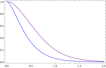
Case I: F​(z)=G​(z)=1βˆ’eβˆ’2​z,z>0,formulae-sequence𝐹𝑧𝐺𝑧1superscript𝑒2𝑧𝑧0F(z)=G(z)=1-e^{-2z},~{}z>0, that is, all the components are have exponential lifetime distributions with parameter 2.
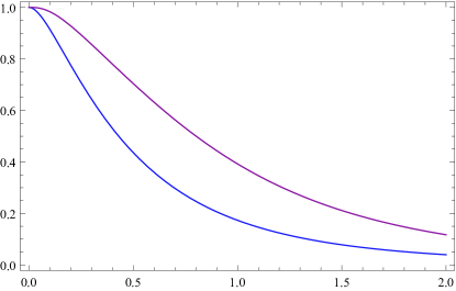
Case II: F​(z)=G​(z)=1βˆ’(1+z)βˆ’2,z>0,formulae-sequence𝐹𝑧𝐺𝑧1superscript1𝑧2𝑧0F(z)=G(z)=1-(1+z)^{-2},~{}z>0, that is, all the components are have Pareto type II lifetime distributions.
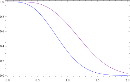
Case III: F​(z)=G​(z)=1βˆ’eβˆ’z2,z>0,formulae-sequence𝐹𝑧𝐺𝑧1superscript𝑒superscript𝑧2𝑧0F(z)=G(z)=1-e^{-z^{2}},~{}z>0, that is, all the components are have Weibull lifetime distributions
Figure 1 depict the graphs of P​(Z2:3>s)𝑃subscript𝑍:23𝑠P(Z_{2:3}>s), P​(T>s)𝑃𝑇𝑠P(T>s) for all the cases.

Refer to caption
(a) Case I
Refer to caption
(b) Case II
Refer to caption
(c) Case III
Figure 1: Plots of P​(Z2:3>s)𝑃subscript𝑍:23𝑠P(Z_{2:3}>s)(blue line) and P​(T>s)𝑃𝑇𝑠P(T>s)(red line) when ΞΈ11=.2;ΞΈ12=.3;ΞΈ21=.5;ΞΈ22=.6;ΞΈ31=.7formulae-sequencesubscriptπœƒ11.2formulae-sequencesubscriptπœƒ12.3formulae-sequencesubscriptπœƒ21.5formulae-sequencesubscriptπœƒ22.6subscriptπœƒ31.7\theta_{11}=.2;~{}\theta_{12}=.3;~{}\theta_{21}=.5;~{}\theta_{22}=.6;~{}\theta_{31}=.7.

It is intuitive that, mean time to failure as well as manufacturing cost of a system will increase if we use a cold standby into the system. To evaluate this changes, we first define the cost per unit of time, which are

CZnβˆ’k+1:n=n​cE​(Znβˆ’k+1:n),subscript𝐢subscript𝑍:π‘›π‘˜1𝑛𝑛𝑐𝐸subscript𝑍:π‘›π‘˜1𝑛C_{Z_{n-k+1:n}}=\frac{nc}{E(Z_{n-k+1:n})},

and,

CT=(n+1)​cE​(T).subscript𝐢𝑇𝑛1𝑐𝐸𝑇C_{T}=\frac{(n+1)c}{E(T)}.

where c𝑐c be the acquisition cost for per component. In Tables I-III, we obtain the values of E​(Znβˆ’k+1:n),𝐸subscript𝑍:π‘›π‘˜1𝑛E(Z_{n-k+1:n}), E​(T),𝐸𝑇E(T), CZnβˆ’k+1:n,subscript𝐢subscript𝑍:π‘›π‘˜1𝑛C_{Z_{n-k+1:n}}, and CTsubscript𝐢𝑇C_{T} when c=1.𝑐1c=1. We see that the cost per unit of time of the system changes significantly (as interpreted in Tables [1-3]).

Table 1: Mean time to failure and mean cost rates for a 2-out-of-3 system with and without a standby component (Case I)
ΞΈ11subscriptπœƒ11\theta_{11} ΞΈ12subscriptπœƒ12\theta_{12} ΞΈ21subscriptπœƒ21\theta_{21} ΞΈ22subscriptπœƒ22\theta_{22} ΞΈ31subscriptπœƒ31\theta_{31} E​(Z2:3)𝐸subscript𝑍:23E(Z_{2:3}) E​(T)𝐸𝑇E(T) CZ2:3subscript𝐢subscript𝑍:23C_{Z_{2:3}} CTsubscript𝐢𝑇C_{T}
00 00 00 00 00 0.4166670.4166670.416667 0.6666670.6666670.666667 7.1999947.1999947.199994 5.9999975.9999975.999997
.1.1.1 .2.2.2 .3.3.3 .4.4.4 .5.5.5 0.4241670.4241670.424167 0.681250.681250.68125 7.0726857.0726857.072685 5.8715595.8715595.871559
.2.2.2 .3.3.3 .5.5.5 .6.6.6 .7.7.7 0.4300000.4300000.430000 0.6883330.6883330.688333 9.3023259.3023259.302325 5.8111405.8111405.811140
Table 2: Mean time to failure and mean cost rates for a 2-out-of-3 system with and without a standby component (Case II)
ΞΈ11subscriptπœƒ11\theta_{11} ΞΈ12subscriptπœƒ12\theta_{12} ΞΈ21subscriptπœƒ21\theta_{21} ΞΈ22subscriptπœƒ22\theta_{22} ΞΈ31subscriptπœƒ31\theta_{31} E​(Z2:3)𝐸subscript𝑍:23E(Z_{2:3}) E​(T)𝐸𝑇E(T) CZ2:3subscript𝐢subscript𝑍:23C_{Z_{2:3}} CTsubscript𝐢𝑇C_{T}
00 00 00 00 00 0.60.60.6 1.005761.005761.00576 555 3.9770923.9770923.977092
.1.1.1 .2.2.2 .3.3.3 .4.4.4 .5.5.5 0.6159310.6159310.615931 1.042691.042691.04269 4.8706754.8706754.870675 3.8362313.8362313.836231
.2.2.2 .3.3.3 .5.5.5 .6.6.6 .7.7.7 0.6290910.6290910.629091 1.0631.0631.063 4.7687854.7687854.768785 3.7629353.7629353.762935
Table 3: Mean time to failure and mean cost rates for a 2-out-of-3 system with and without a standby component (Case III)
ΞΈ11subscriptπœƒ11\theta_{11} ΞΈ12subscriptπœƒ12\theta_{12} ΞΈ21subscriptπœƒ21\theta_{21} ΞΈ22subscriptπœƒ22\theta_{22} ΞΈ31subscriptπœƒ31\theta_{31} E​(Z2:3)𝐸subscript𝑍:23E(Z_{2:3}) E​(T)𝐸𝑇E(T) CZ2:3subscript𝐢subscript𝑍:23C_{Z_{2:3}} CTsubscript𝐢𝑇C_{T}
00 00 00 00 00 0.8566440.8566440.856644 1.219981.219981.21998 3.5020543.5020543.502054 3.2787423.2787423.278742
.1.1.1 .2.2.2 .3.3.3 .4.4.4 .5.5.5 0.8632280.8632280.863228 1.223711.223711.22371 3.4753273.4753273.475327 3.2687483.2687483.268748
.2.2.2 .3.3.3 .5.5.5 .6.6.6 .7.7.7 0.8679080.8679080.867908 1.223081.223081.22308 3.4565873.4565873.456587 3.2704323.2704323.270432

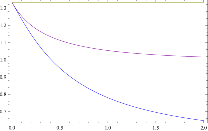
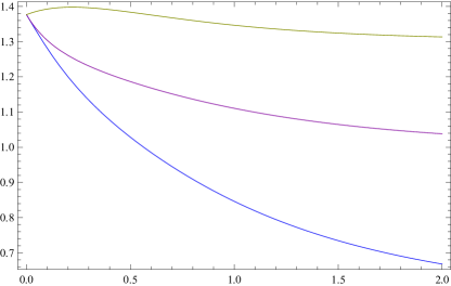
Now, we numerically examine how the component’s dependence effects the shape of mean residual life functions. We obtain the plots of Ξ¨1​(t)subscriptΞ¨1𝑑\Psi_{1}(t), Ξ¨2​(t),subscriptΞ¨2𝑑\Psi_{2}(t), and Ξ¨3​(t)subscriptΞ¨3𝑑\Psi_{3}(t) for the system defined by equation (29) when F​(z)=G​(z)=1βˆ’eβˆ’z,z>0formulae-sequence𝐹𝑧𝐺𝑧1superscript𝑒𝑧𝑧0F(z)=G(z)=1-e^{-z},~{}z>0 for the following cases:
Case I: ΞΈ11=0;ΞΈ12=0;ΞΈ21=0;ΞΈ22=0;ΞΈ31=0formulae-sequencesubscriptπœƒ110formulae-sequencesubscriptπœƒ120formulae-sequencesubscriptπœƒ210formulae-sequencesubscriptπœƒ220subscriptπœƒ310\theta_{11}=0;~{}\theta_{12}=0;~{}\theta_{21}=0;~{}\theta_{22}=0;~{}\theta_{31}=0
Case II: ΞΈ11=.2;ΞΈ12=.3;ΞΈ21=.5;ΞΈ22=.6;ΞΈ31=.7formulae-sequencesubscriptπœƒ11.2formulae-sequencesubscriptπœƒ12.3formulae-sequencesubscriptπœƒ21.5formulae-sequencesubscriptπœƒ22.6subscriptπœƒ31.7\theta_{11}=.2;~{}\theta_{12}=.3;~{}\theta_{21}=.5;~{}\theta_{22}=.6;~{}\theta_{31}=.7
In Figure 2, we see that Ξ¨3​(t)subscriptΞ¨3𝑑\Psi_{3}(t) do not change along time for Case I, that is, when components are independent which is due to the memoryless property of exponential distribution. But it is not true when components are dependent (Case II). We see that Ξ¨3​(t)subscriptΞ¨3𝑑\Psi_{3}(t) first increase and then decrease for Case II. We observe that Ξ¨1​(t)≀Ψ2​(t)≀Ψ3​(t)subscriptΞ¨1𝑑subscriptΞ¨2𝑑subscriptΞ¨3𝑑\Psi_{1}(t)\leq\Psi_{2}(t)\leq\Psi_{3}(t) for all the cases. It is also see that Ξ¨1​(t),subscriptΞ¨1𝑑\Psi_{1}(t), and Ξ¨2​(t)subscriptΞ¨2𝑑\Psi_{2}(t) are decreasing over time.

Refer to caption
(a) Case I
Refer to caption
(b) Case II
Figure 2: Plots of Ξ¨1​(t)subscriptΞ¨1𝑑\Psi_{1}(t)(blue line), Ξ¨2​(t)subscriptΞ¨2𝑑\Psi_{2}(t)(red line) and Ξ¨3​(t)subscriptΞ¨3𝑑\Psi_{3}(t)(brown line) for 2-out of -3 system when F​(z)=G​(z)=1βˆ’eβˆ’z,z>0,formulae-sequence𝐹𝑧𝐺𝑧1superscript𝑒𝑧𝑧0F(z)=G(z)=1-e^{-z},~{}z>0,.

4 Conclusions

Here, we study a kπ‘˜k-out-of-n𝑛n system consisting of n𝑛n exchangeable components equipped with a cold standby component when all the components are assumed to be dependent. An exact expression has been obtained for the survival function of the system in terms of copula functions. We have also presented explicit expressions for three different mean residual functions of the system. We illustrate the theoretical results given in this article. The results established in this article generalize the results in Eryilmaz, [7] as pointed out in Remark 1, Remark 4 and Corollary 2.

References

  • Asadi and Bayramoglu, [2005] Asadi, M. and Bayramoglu, I. (2005). A note on the mean residual life function of a parallel system. Communications in Statistics-Theory and Methods, 34(2):475–484.
  • Asadi and Bayramoglu, [2006] Asadi, M. and Bayramoglu, I. (2006). The mean residual life function of a k-out-of-n structure at the system level. IEEE Transactions on Reliability, 55(2):314–318.
  • Bairamov etΒ al., [2002] Bairamov, I., Ahsanullah, M., and Akhundov, I. (2002). A residual life function of a system having parallel or series structures. Journal of Statistical Theory and Applications, 1(2):119–132.
  • Bairamov and Parsi, [2011] Bairamov, I. and Parsi, S. (2011). Order statistics from mixed exchangeable random variables. Journal of computational and applied mathematics, 235(16):4629–4638.
  • Barlow and Proschan, [1975] Barlow, R.Β E. and Proschan, F. (1975). Statistical theory of reliability and life testing: probability models. Silver Spring, MD: Madison.
  • EryΔ±lmaz, [2011] EryΔ±lmaz, S. (2011). Dynamic behavior of k-out-of-n: G systems. Operations Research Letters, 39(2):155–159.
  • Eryilmaz, [2012] Eryilmaz, S. (2012). On the mean residual life of a k-out-of-n: G system with a single cold standby component. European Journal of Operational Research, 222(2):273–277.
  • Eryilmaz, [2014] Eryilmaz, S. (2014). A study on reliability of coherent systems equipped with a cold standby component. Metrika, 77(3):349–359.
  • Eryilmaz and Ozkut, [2020] Eryilmaz, S. and Ozkut, M. (2020). Optimization problems for a parallel system with multiple types of dependent components. Reliability Engineering & System Safety, 199:106911.
  • Eryilmaz and Tank, [2012] Eryilmaz, S. and Tank, F. (2012). On reliability analysis of a two-dependent-unit series system with a standby unit. Applied Mathematics and Computation, 218(15):7792–7797.
  • Levitin etΒ al., [2014] Levitin, G., Xing, L., and Dai, Y. (2014). Cold vs. hot standby mission operation cost minimization for 1-out-of-n systems. European Journal of Operational Research, 234(1):155–162.
  • Li and Zhao, [2006] Li, X. and Zhao, P. (2006). Some aging properties of the residual life of kπ‘˜k-out-of-n𝑛n systems. IEEE Transactions on Reliability, 55(3):535–541.
  • Mirjalili etΒ al., [2017] Mirjalili, A., Sadegh, M.Β K., and Rezaei, M. (2017). A note on the mean residual life of a coherent system with a cold standby component. Communications in Statistics-Theory and Methods, 46(20):10348–10358.
  • Navarro etΒ al., [2005] Navarro, J., Ruiz, J.Β M., and Sandoval, C.Β J. (2005). A note on comparisons among coherent systems with dependent components using signatures. Statistics & Probability Letters, 72(2):179–185.
  • Navarro etΒ al., [2007] Navarro, J., Ruiz, J.Β M., and Sandoval, C.Β J. (2007). Properties of coherent systems with dependent components. Communications in Statisticsβ€”Theory and Methods, 36(1):175–191.
  • Navarro and Rychlik, [2010] Navarro, J. and Rychlik, T. (2010). Comparisons and bounds for expected lifetimes of reliability systems. European Journal of Operational Research, 207(1):309–317.
  • Nelsen, [2007] Nelsen, R.Β B. (2007). An introduction to copulas. Springer Science & Business Media.
  • Roy and Gupta, [2019] Roy, A. and Gupta, N. (2019). Reliability of a coherent system equipped with two cold standby components. Metrika, pages 1–21.
  • Roy and Gupta, [2020] Roy, A. and Gupta, N. (2020). Reliability function of k-out-of-n system equipped with two cold standby components. Communications in Statistics-Theory and Methods, pages 1–20.
  • Sadegh, [2011] Sadegh, M.Β K. (2011). A note on the mean residual life function of a coherent system with exchangeable or nonidentical components. Journal of Statistical Planning and Inference, 141(9):3267–3275.
  • Sadegh, [2016] Sadegh, M.Β K. (2016). Distribution of order statistics for exchangeable random variables.
  • Wang, [2016] Wang, Y. (2016). Conditional k-out-of-n systems with a cold standby component. Communications in Statistics-Theory and Methods, 45(21):6253–6262.
  • Yongjin etΒ al., [2018] Yongjin, Z., Youchao, S., Longbiao, L., and Ming, Z. (2018). Copula-based reliability analysis for a parallel system with a cold standby. Communications in Statistics-Theory and Methods, 47(3):562–582.
  • Zhao etΒ al., [2012] Zhao, P., Chan, P.Β S., and Ng, H. K.Β T. (2012). Optimal allocation of redundancies in series systems. European Journal of Operational Research, 220(3):673–683.
  • Zhao etΒ al., [2017] Zhao, P., Zhang, Y., and Chen, J. (2017). Optimal allocation policy of one redundancy in a n-component series system. European Journal of Operational Research, 257(2):656–668.