Machine learning of Kondo physics using variational autoencoders and symbolic regression
Abstract
We employ variational autoencoders to extract physical insight from a dataset of one-particle Anderson impurity model spectral functions. Autoencoders are trained to find a low-dimensional, latent space representation that faithfully characterizes each element of the training set, as measured by a reconstruction error. Variational autoencoders, a probabilistic generalization of standard autoencoders, further condition the learned latent space to promote highly interpretable features. In our study, we find that the learned latent variables strongly correlate with well known, but nontrivial, parameters that characterize emergent behaviors in the Anderson impurity model. In particular, one latent variable correlates with particle-hole asymmetry, while another is in near one-to-one correspondence with the Kondo temperature, a dynamically generated low-energy scale in the impurity model. Using symbolic regression, we model this variable as a function of the known bare physical input parameters and “rediscover” the non-perturbative formula for the Kondo temperature. The machine learning pipeline we develop suggests a general purpose approach which opens opportunities to discover new domain knowledge in other physical systems.
I Introduction
Experimental spectra such as those obtained by x-ray absorption, resonant inelastic x-ray scattering, optics, and angle resolved photoemission provide detailed information about the system response for strongly correlated materials Damascelli et al. (2003); Valla et al. (1999); Dean et al. (2016). Spectroscopy techniques typically involve the absorption and emission of energy that induce transitions between states of the material. These processes are generally expensive/time-consuming to measure or simulate, and are also difficult to interpret, as they involve complicated many-body interactions.
A particularly important quantity of interest is the one-particle Green’s function, which characterizes the many-body system’s response to the injection or removal of an electron Mahan (2013). The spectral function, completely encodes through Kramers-Kronig relations and is generally experimentally measurable. Its peaks and line shapes encode non-trivial many-body features such as renormalized energy scales, the many-body eigenspectrum, and quasiparticle lifetimes. However, interpretation of spectral data is often a significant and system-dependent challenge requiring the combination of experimental spectroscopy, educated guesses, and informed theoretical analysis. In this paper, we develop a data-driven representation learning workflow for generating physical insight in the form of analytic expressions from a collection of physical data, and demonstrate its power in this context of spectral interpretation.
The goal of representation learning techniques is to automatically extract a low-dimensional set of features that describe the trends and variations of a collection of high-dimensional raw data Bengio et al. (2013). Unlike supervised learning, each datapoint remains unlabeled, and the goal is to learn the underlying structure of a dataset as opposed to a 1-to-1 mapping. While there exist many viable techniques for representation learning, we focus here on the recently prominent approach of training autoencoders Tschannen et al. (2018). These are feed-forward neural networks trained to approximate the identity function , where the network has a restricted functional form that involves a low-dimensional “bottleneck” (latent space). The intention is that the latent space should distill the information most necessary for accurate reconstruction of the input. In this work, we use a stochastic variant called the variational autoencoder (VAE) Kingma and Welling (2014); Doersch (2021) which has been empirically found to improve interpretability of the latent space components Higgins et al. (2017).
Autoencoder-based unsupervised learning has begun to see wide use in the physical sciences in various applications such as generating realistic data following a learned distribution Martínez-Palomera et al. (2020); Otten et al. (2021), collider event anomaly detection Farina et al. (2020); Cerri et al. (2019), phase identification Wetzel (2017); Kottmann et al. (2020), and as a tool in inverse optimization problems Samarakoon et al. (2020). However, the prospect of using this technique for the discovery of interpretable physical features has been explored only very recently Routh et al. (2021); Lu et al. (2020); Kalinin et al. (2021). In these works, VAEs were found to produce remarkably interpretable low-dimensional features characterizing datasets Routh et al. (2021); Kalinin et al. (2021), even near-perfectly reproducing known physical parameters in controlled settings Lu et al. (2020). But it is not clear how to best train these models or connect them to unknown physics without significant prior knowledge. We here explore these questions and demonstrate a complete pipeline to train interpretable VAEs, and additionally propose a novel application of symbolic regression Schmidt and Lipson (2009); Bongard and Lipson (2007) to discover analytic expressions describing the captured features in terms of a set of known physical quantities.
The present study focuses on a dataset of spectral response functions from the famous single impurity Anderson model (SIAM) Anderson (1961). The SIAM model describes a single quantum impurity (or quantum dot) embedded in a non-interacting bath of fermions. Despite this model’s simplicity, it is a key tool in the examination of strongly correlated low-energy phenomena such as Kondo screening and the Kondo resonance. We have selected this system as it is well-understood and numerically inexpensive to evaluate non-perturbatively. Thus the creation of a large, varied dataset for machine learning (ML) purposes is achievable. Moreover, the dynamically generated low-energy regime of this model is well-known to be non-analytically related to the bare parameters, presenting a non-trivial set of features for the VAE to unravel.
The outline of the paper is as follows. We first introduce the model and review VAEs in the context of spectral function reconstruction. Then, we demonstrate that training VAEs with varying regularization strengths reveals a “critical” number of dimensions needed to characterize a dataset. We find that each dimension of the latent space corresponds to a key physical descriptor for the set of SIAM spectral functions. The automatically discovered descriptors include (a) the Kondo temperature Kondo (1964), (b) a measure of particle-hole asymmetry, and (c) the presence of competing energy scales. Finally, we propose and demonstrate the use of symbolic regression to extract analytic expressions for these emergent physical descriptors.
II Methodology
II.1 Overview of physical system
We examine the spectral functions of the prototypical SIAM with Hamiltonian
| (1a) | |||||
| where | |||||
| (1b) | |||||
| (1c) | |||||
| (1d) | |||||
The impurity (imp) constitutes a particle with spin at energy level relative to the Fermi surface in the presence of an external magnetic field of strength Double occupation is penalized by the Coulomb repulsion energy The impurity couples to the bath via characterized by the hybridization function , where is the density of states and represents the hopping elements between the impurity and bath level at energy relative to the Fermi energy, with the normalized bath levels obeying . The fermionic bath is described by In this work we examine the SIAM spectral functions for constant hybridization functions within the bandwidth, , i.e. the so-called “box” distribution, where is the Heaviside step function. Hence the model Hamiltonian (1) is particle-hole symmetric for . Unless otherwise noted, all energies are in units of the half-bandwidth . We also set .
The spectral function represents the impurity’s local density of states, as derived from the time-dependent retarded fermionic Green’s function after Fourier transform from time to frequency , with denoting the thermal average. At finite , we pick an arbitrary but fixed spin orientation throughout. The features of the spectral data are well-known analytically: At , the spectral data shows peaks around and of width (the so-called Hubbard side peaks) which are trivially related to bare energies of the Hamiltonian, as well as a peak pinned around which derives from low-energy particle-hole excitations mediated by the Kondo interaction. The width of the latter peak defines the dynamically generated low-energy Kondo scale , where for the Kondo regime typically . This peak gets suppressed by temperature , and becomes strongly asymmetric in the spin-resolved case when applying a magnetic field .
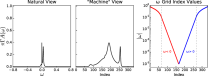
Each spectral function is generated by the numerical renormalization group (NRG) Wilson (1975); Bulla et al. (2008); Weichselbaum and von Delft (2007); Weichselbaum (2012), and is controlled by five independent physical parameters: and (the temperature). Values for each of the parameters are chosen randomly according to the Anderson set procedures presented in Ref. Sturm et al. (2021). To normalize the spectra to roughly comparable absolute scales, we utilize our knowledge of the Friedel-sum rule to motivate a normalization of the spectra to . As a second element of human input, we choose to sample the spectra on a fixed linear-logarithmic frequency grid to form the inputs to the VAE. This frequency sampling, as detailed in Fig. A9 and Ref. Sturm et al. (2021), allows variations of the dynamically-generated low-energy scale at exponentially small to be clearly resolved.
We utilize the smallest physical energy (SPE) value, to define two datasets with different effective dimensionalities in their respective physical parameter spaces. Here is the Kondo temperature known analytically at as Haldane (1978); Tsvelick and Wiegmann (1983)
| (2) |
The first dataset, referred to as the -dominated dataset, is constrained to spectral functions within the parameter space 111This cutoff in was heuristically chosen to both minimize the effects of while keeping the dataset roughly the same size as our full-parameter dataset., with a total of about spectral functions present in the training set. Spectra from this dataset are thus effectively described by three parameters . The second dataset is unconstrained, such that the SPE is equally controlled by , resulting in a total of five parameters. We refer to this dataset as the full-parameter dataset, with a total of about spectral functions. The random sampling of these two datasets from the data pool of Ref. Sturm et al. (2021) is done independently, so that the first dataset is not a subset of the second.
II.2 Overview of variational autoencoders
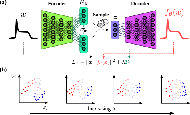
The core idea of all autoencoder-based architectures is to learn an effective compression of a dataset by learning a parameterized form of the identity function with an informational bottleneck. As shown in Fig. 1, VAEs do this using two components: the encoder and the decoder. A standard fully-connected encoder compresses the input through a series of affine transformations followed by point-wise nonlinear functions. The output of the th layer is given by
| (3) |
where is a nonlinear activation function acting element-wise on its input. All encoder layers rely upon the rectified linear unit activation function (), except the final layer which uses the identity function. The encoder consists of total hidden layers.
The weight matrices and bias vectors are all free, learned parameters which we collectively denote as . In the encoding stage, the number of activations steadily decreases, forcing the model to learn consecutively lower-dimensional representations of the input data. We denote the final values output by the encoder as , with an architectural hyperparameter.
VAEs are distinguished from traditional autoencoders in the sense that these final activations no longer represent a single compressed point encoding the input . Instead, these activations are used to parameterize a normal distribution with mean vector and log-variances . The -dimensional space this distribution lives in is called latent space, with each dimension being a latent variable.
On any given forward pass, the encoder maps , then samples from the obtained multivariate normal distribution , where diag constructs a diagonal matrix with along the diagonal. The sampled -component latent vector is finally passed to the decoder which generates the reconstruction . As is common practice, for simplicity and speed we only sample a single for each input per forward pass during training. Combined with the training procedure outlined in the next section, this sampling process forces the VAE to acquire the notion of continuity and statistical independence in the learned latent space. Thus, it is generally found that VAEs learn more “meaningful”, statistically disentangled representations than standard autoencoders Higgins et al. (2016).
The decoder is a deterministic fully-connected network of hidden layers from the sampled latent variables back to the original input space, generally following a reversed structure to the encoder as shown in Fig. 1. The goal is for the decoded output to be a minimally-lossy reconstruction for the original input . We denote the full VAE action as , which is a random variable due to the sampling within latent space. As before, all layers of the decoder except for the last use the ReLU activation function. For the last layer of the decoder we utilize as the activation function to enforce positivity of in a smooth manner. In this work, all networks studied have , with hidden layer sizes manually tuned to (reversed for the decoder, except for ). We found to be sufficiently large to saturate reconstruction performance on both datasets (see App. A).
II.3 Loss functions and training
The parameters of the VAE are learned during training so as to minimize the objective loss function, This loss originates as a bound on the log-likelihood of the distribution defined by the VAE (see Sec. A.2), and can be written in our case as:
| (4) |
where explicit dependence on the dataset has been suppressed for brevity. The two contributions are defined as
| (5a) | ||||
| (5b) | ||||
and are referred to as the reconstruction loss and the Kullback-Leibler divergence (KLD), respectively, each averaged across the dataset of size .
measures the expected squared error between the input and the reconstructed approximation , with the expectation over samples of in latent space. Meanwhile, measures the average KLD between the distribution in latent space predicted by the encoder, and a Gaussian distribution with zero mean and unit variance Kingma and Welling (2014). For the case in Eq. (5b), this term is known analytically as a function of and and can be expressed as a sum over latent variables,
| (6) |
In the Bayesian sense, is to be interpreted as a prior for the latent space distribution, and we penalize the network for deviating from this prior Doersch (2021). In practice, this regularizes the latent space learned by the model by pushing it to only use as much of the latent space as necessary to perform reconstruction well, as well as pushing the latent variables to be statistically independent. The relative strength of the KL divergence is tuned by the regularization hyperparameter The appropriate scale of is set by the input and latent dimensionality as well as the overall scale of the inputs, but in practice must be tuned by hand (see App. A.2). During training, we find it useful to anneal the regularization strength by starting training with and slowly increasing it until reaching the final (reported) value Bowman et al. (2016). We perform this optimization by standard minibatch training using the ADAM optimizer Kingma and Ba (2015) (see App. A.3).
III Results & Discussion
III.1 Training results
To search for interpretable models that capture meaningful aspects of the dataset, we first train a collection of VAEs at various final regularization strengths For each value of , we train three models 222We observe that the variance in final losses between trained models is negligible for the purposes of constructing the loss curves in Fig. 2(a). However, due to multiple local minima, at some there is occasionally active latent in the final model. and measure the final reconstruction and KLD losses, averaged across the dataset. Plotting these against each other in Fig. 2(a) demonstrates the fundamental reconstruction-regularization trade-off. Ideally, we want to minimize both losses to obtain a model which captures the dataset with a simply structured, low-dimensional latent space.
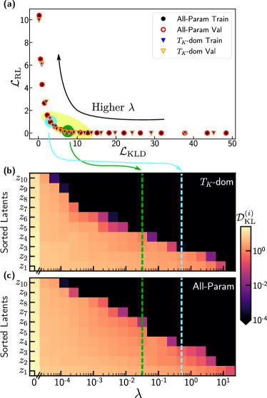
An interesting feature of this trade-off is a pronounced corner region (highlighted in yellow) where is minimal. Moving towards large only improves modestly, but incurs a large sacrifice in reconstruction performance. Since measures the amount of information encoded into the latent space relative to the unit Gaussian prior Doersch (2021), we interpret the region marked in yellow as where the “critical” amount of information is present in the model. Beyond this point, the information capacity of the model dips below what is necessary to capture the trends contained in the dataset. In Sec. A.2, we show that this critical region is clearly identifiable as an inflection point in log-log space. This is understandable as a local optimum in , which is a scale-invariant measurement of the tradeoff magnitude.
We can gain further insight into these models by observing how the total is spread across the latent variables for each as shown in Fig. 2(b). Here, and for the rest of the paper, we sort the latent variables by their respective average in decreasing order. Increasing the regularization strength has the effect of entirely deactivating some of the latent neurons, resulting in them simply predicting the prior irrespective of the input , thus achieving a nearly-zero KL loss
As visualized in Fig. 2(b), the number of active neurons in latent space is rather sharply defined for finite . We find that at the onset of the “critical” region, the number of active neurons nearly matches the number of free physical parameters describing the relevant training dataset. Three physical parameters characterize the -dominant dataset, and we observe that the number of active neurons in the relevant trained model transitions from . Similarly, the full-parameter dataset has two additional underlying parameters , and the trained model transitions from active . We find however, that these discovered latents do not correlate well one-to-one with the bare Hamiltonian parameters, reflecting that bare parameters are not necessarily the best way of characterizing the dataset.
A second desired effect of the KL regularization is to push each dimension of the latent space to correspond a “disentangled” feature Higgins et al. (2016) which carries a distinct physical meaning. Ideally, this results in each latent variable learning a statistically independent feature, i.e. . In App. A, we define a heuristic metric of success towards this goal as a normalized sum of off-diagonal elements of the latent covariance matrix, and show that statistical independence indeed improves as is increased. To obtain simple interpretable models which are well-disentangled and low-dimensional while also capable of reconstructing spectra with reasonable accuracy, we train beyond the critical at (cyan markers in Fig. 2) where only active remain for the -dominated and full-parameter sets, respectively. Since these models have fewer active than the number of free physical parameters we know to be present, we are effectively forcing the models to learn high-level combinations of these parameters, corresponding to the most important physical variations in the dataset. (See App. D for views of lower-regularization models).
III.2 Interpretation of the latent spaces
We first investigate VAE models trained to reconstruct spectral functions from the -dominated regime, . To analyze the latent space structure post-training, we disable the random sampling by setting . Hence, when discussing distributions below, we are referring the distribution of in the latent space across all in the training dataset. For the -dominated dataset, we find that well-trained models at have all but two bottleneck neurons deactivated [cf. Fig. 2(b)].
To understand the nature of this two-dimensional active latent space, we scan the values of the two active latents and analyze how the reconstructed spectral functions evolve. Examples are shown in Fig. 3, where we sweep the two active neurons in the range corresponding to two standard deviations of the KL prior. We also provide the respective ground-truth input NRG spectra which encodes the closest -value. We observe that the reconstructed spectra smoothly evolve as we move around this space, reconstructing plausible intensity profiles. However, due to the reconstruction vs. KL loss trade-off, this model misses the fine details of the small Hubbard-like side peaks at large energies for large negative .
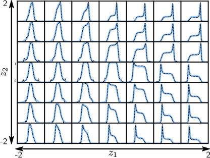
Fig. 3 shows that increasing corresponds to a broadening and flattening of the central Kondo peak in the spectral function. Physically, we infer that this feature relates to the Kondo temperature which sets the overall energy scale associated with this peak. Meanwhile, learned the physical particle-hole asymmetry of the SIAM Hamiltonian. For any , the transformation roughly results in the reflection of the decoded spectral function around .
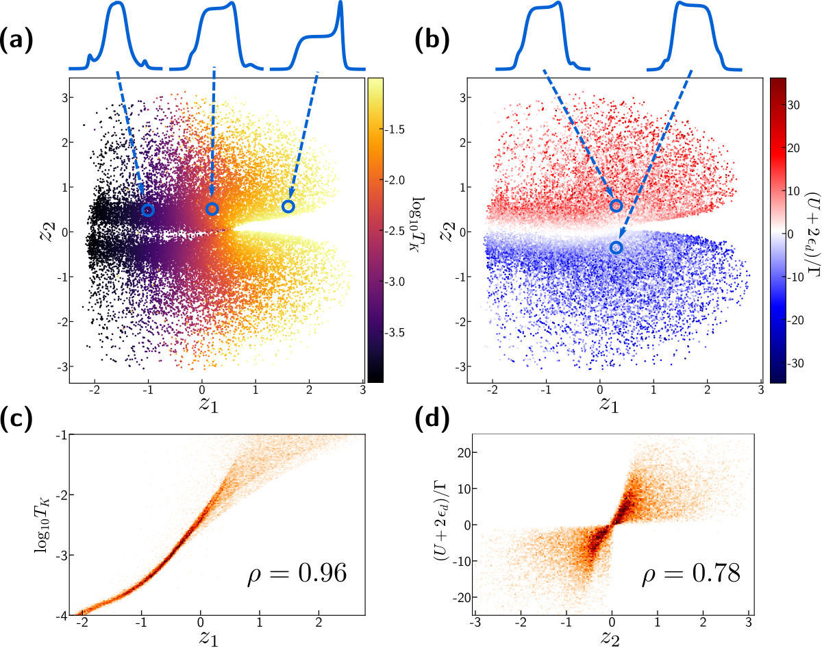
These correspondences are summarized in Fig. 4 where we plot the distribution of the training dataset in latent space and color the points according to relevant physical parameters. We find a remarkably high correlation between the first latent dimension and [Fig. 4(a,c)]. Furthermore, in Fig. 4(b,d) we see that can be associated with the ratio which characterizes the particle-hole asymmetry in the SIAM. These strong correlations indicate that the VAE has successfully learned the dominant physical features characterizing the dataset.
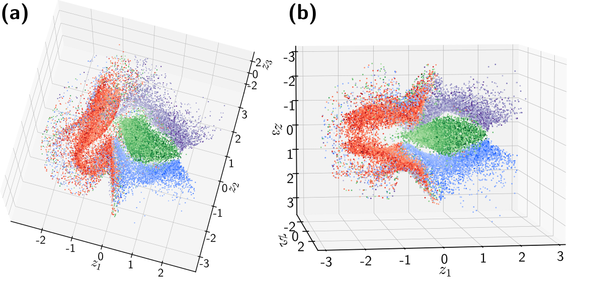
We now investigate VAEs trained on the full five-parameter dataset, which shares the SPE control equally between . We again choose to examine models from the cyan region of Fig. 2, where we see only three latents remain active. Similar to Figs. 3,4, we simultaneously examine both direct generative scans of the learned latent space (Fig. 5), as well as the dataset distribution in the full three-dimensional latent space (Fig. 6). Interestingly, we now find that rather than one globally continuous manifold, our models tend to break the dataset into multiple distinct clusters which only separately form continuous spaces. This decomposition can be directly connected to certain physical properties in the dataset. In Fig. 6(c), we show how the learned latent space decomposes into four disconnected clusters, each of which is characterized by a different physical parameter that dominates the smallest physical energy . Additional views of these data are available in App. B.
When all (center column of Fig. 5), the height of the spectral function is reduced (indicative of finite temperature ), the spectrum is left-right (particle-hole) symmetric, and shows no Hubbard side peaks (indicative of larger ). Now when varying , this changes the height of the spectral function while keeping it largely symmetric. Therefore controls the underlying temperature, which is also reinforced by observing that is in a -dominated regime, as seen by the green data in Fig. 6 and Fig. A12. On the other hand, large positive switches towards the -dominated low- regime (red data in Fig. 6). Additionally, we find that controls the width of the spectral function’s central peak. As such, it is directly connected to the absolute energy scale describing each spectral function, as shown in Fig. 6(b) and Fig. A12.
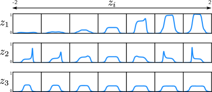
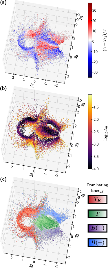
Meanwhile, controls much of the asymmetry of the spectral function around . At small , , characterizes the particle-hole asymmetry [see Fig. 6(a)]. Magnetic fields also break the inversion symmetry of the spin-resolved spectral data. Hence competes with the effect of particle-hole asymmetry controlled by . For large therefore the latent space switches to a -dominated domain (see blue data in Fig. 6(c)) which goes hand in hand with a sign change in .
Due to the rather strong regularization, the examined VAE does not fully capture all of the features of the dataset. In particular, this examined model focuses on the central Kondo peak features, but tends to miss the sharp Hubbard-like side peaks appearing in the high- and high- regions. In Fig. A16 of the Appendix, we examine VAEs trained with weaker regularization that do successfully capture these side peaks, but are more difficult to interpret.
To gain confidence that our VAEs learn meaningful representations, an important question is whether the structures of the data manifolds discovered by these separately-trained VAEs are consistent with each other. The -dominated dataset by its construction lies entirely within the red high- “bulb” of the full-parameter dataset at large in Fig. 6, seen to be a roughly two-dimensional manifold. Do continuous paths within the two-dimensional latent space of the -dominated model correspond to continuous paths on this bulb?
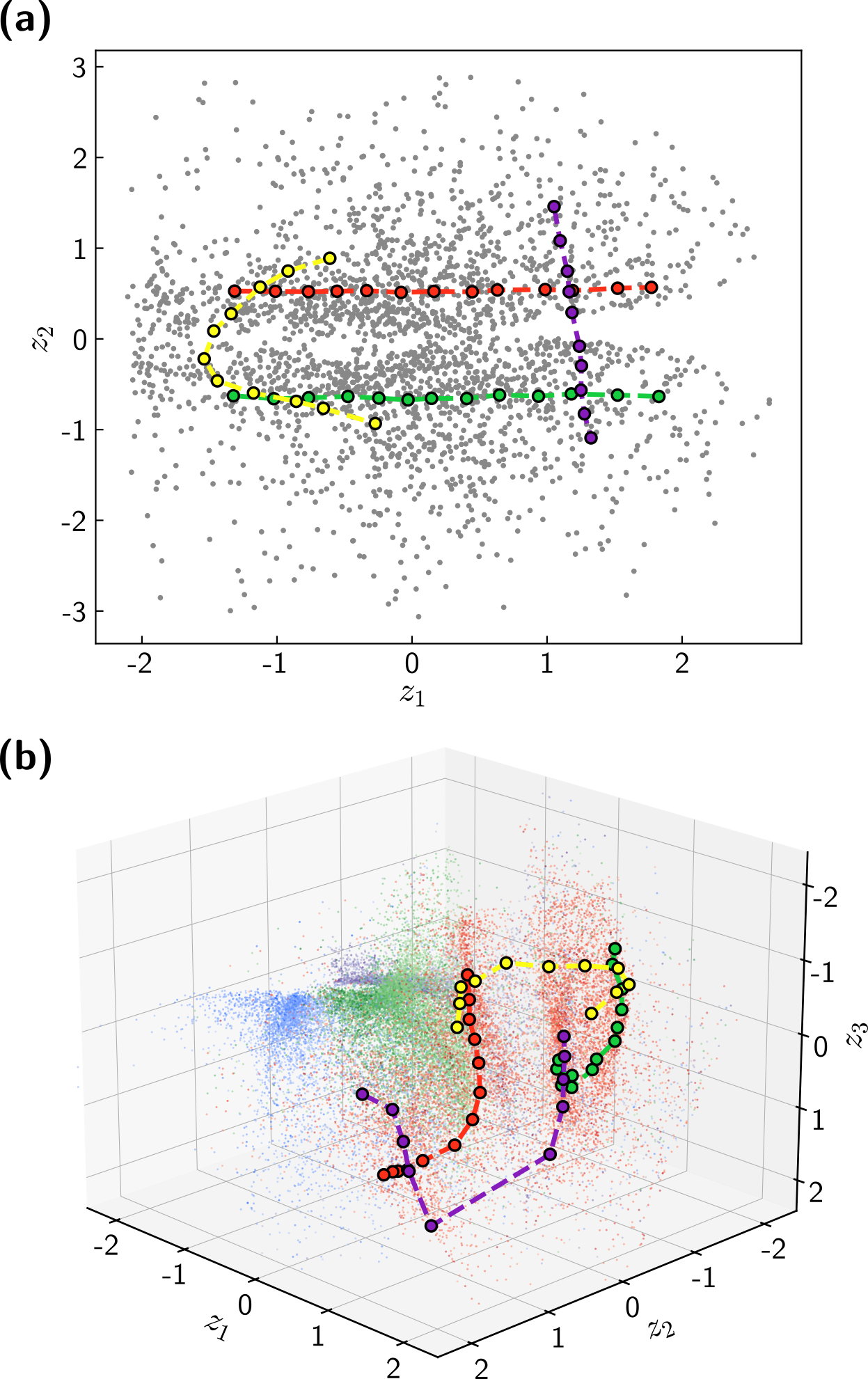
To answer this, we start by choosing several paths of points in the latent space of the -dominated model, as shown in Fig. 7(a). The red and green paths are chosen to be at roughly constant and opposite values of the particle-hole asymmetry , extending primarily along . The yellow and purple paths are chosen to span the two particle-hole asymmetric lobes, with the yellow path tracing through a seemingly connected region while the purple path crosses an apparent void. By feeding these same spectra into the encoder of the full-parameter VAE, we can retrace these paths in its learned three-dimensional activate latent space.
As shown in Fig. 7(b), we indeed find that the mapped path demonstrates consistency in the sense of continuity and qualitative topology between the two models. The two-dimensional -dominated latent space is continuously “wrapped” into the red frontal bulb of the full-parameter latent space. Interestingly, the purple path maintains its single discontinuity in the extended space, occurring exactly when the path jumps between the two particle-asymmetric lobes. This analysis further confirms that these learned latent spaces are all meaningfully connected to the same underlying physics, regardless of which subset of the data is seen by the model.
III.3 Symbolic regression to extract physical descriptors
Much of our previous analysis depended on having the physical foresight to determine explicit physical features which could correspond to various dimensions in latent space. For use in machine learning-aided discovery, we require some means to automatically extract these features given a trained VAE. We propose a potential route towards this goal using symbolic regression (SR) Schmidt and Lipson (2009); Bongard and Lipson (2007). We assume knowledge of a set of physical parameters associated with the generation of each spectral function (and hence each latent vector ). In our case will be the Hamiltonian parameters of Eq. (1), while in experimental settings these may be, e. g., the temperature and applied pressure. Using SR, we can then search through the space of analytic expressions of to find those which best describe each learned latent . Intuitively, we hope that the information the VAE has chosen to keep in the bottleneck will inform us of effective combinations of which correspond to meaningful physical quantities. While SR has been previously investigated as a way to understand the transformation learned by the network Cranmer et al. (2020), our goal here is different – the network has never seen , and we are using SR to inform us how the critical bottleneck information relates to the original generative factors .
In SR, functions are represented as syntax trees, where operations appear as interior nodes, and parameters appear as leaves [see Fig. 8(c,d) for examples]. We define the class of representable functions by specifying a list of unary and binary functions which are allowed to appear in these trees. In this work, we limit this list to include the standard binary arithmetic operations as well as unary negation and inversion. Then, we phrase the objective as finding the symbolic function in this class which maximizes the Pearson correlation coefficient with an individual latent :
| (7) |
where expectation values indicate means with respect to the dataset and ’s are standard deviations of the subscripted variables. We note that this objective function is invariant under an overall scale factor or constant shift of either the ’s or ’s. To bias the optimization process towards simple expressions, an additional penalty is introduced of the form where is a hyperparameter and is the number of nodes in the syntax tree.
One symbolic function is regressed per active latent dimension We utilize the gplearn library Stephens (2015), which performs this search using genetic algorithm techniques Pal and Wang (1996). At the beginning of the regression, a large number of trial symbolic functions are added to a population by constructing random syntax trees up to a given finite depth. At each stage, the worst-performing functions are discarded and new functions are generated by randomly modifying the best-performing functions using biologically inspired mutation and crossover operations. Mutation operations randomly replace nodes with alternate operations or parameters, while crossover operations mix subtrees between functions. Iterating these processes improves the general performance of the entire population until reaching some plateau. While this approach is generally sensitive to the specification of various hyperparameters controlling mutation/crossover probabilities, we find that other than increasing the population size to and the program length penalty to , the default package parameters perform well for our purposes.
We apply this approach to extract explicit functions describing the latent dimensions of VAEs trained on the -dominated dataset in Fig. 4. Since in this dataset, the available Hamiltonian parameters which may appear in our regressed functions are . We find it useful to enforce unitless expressions by setting the available leaf nodes in the regression to be the unitless ratios . We regress two functions to obtain symbolic expressions which correlate well with the two active latent variables , resulting in Fig. 8.
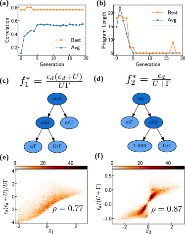
Remarkably, we consistently find the function automatically discovered as describing to be (syntax tree in Fig. 8(c)), which is precisely [Eq. (2)] up to a logarithmic correction of inexpressible in terms of our chosen operator set, and a constant coefficient/shift which leaves the correlation invariant. While the symbolic regression does not directly inform us that it has learned the of a relevant quantity, this can be inferred from the fact that the data has been presented to the VAE on a logarithmic energy grid. The correlation between this optimized function and was found to be (Fig. 8(e)) while the correlation between the full and is , indicating that these logarithmic corrections explain a small but notable fraction of the correlation. We find that expanding the operator set to include and using bare input parameters tends to recover these key logarithmic factors, but also generates a handful of extraneous terms. We anticipate that careful tuning or advanced approaches producing Pareto frontiers Deb et al. (2002) would successfully filter through this excess, though are beyond the scope of this work.
The obtained function which correlates best with was consistently found to be , which differs from our “knowledgable” guess for particle-hole asymmetry of . In fact, is found to have a greater correlation with than does, showing that this is not a failure of the regression. This instead can be explained from the observation that the latent space is not very well-structured at large , as seen from the large spread in Fig. 4(b,d). While the VAE can accurately perform the correct ordering of spectral functions which slightly deviate from the particle-hole symmetric point, it seems to not focus as much on getting this ordering correct between very asymmetric curves. Motivated by this observation, we find that if the symbolic regression is restricted to regress only the high-density region of points with , it then does reliably recover the “ideal” expression of .
IV Discussion
The results of this work demonstrate a promising avenue towards machine-assisted physical discovery. Given an unlabeled set of data generated through some physical process, our work shows how methods from unsupervised machine learning can automatically extract physically-meaningful structure. VAEs accomplish this by discovering a small set of disentangled features parameterizing a low-dimensional manifold which can be used to reconstruct the data faithfully. However, alternate dimensionality reduction techniques can also stand in this place (see App. C). Symbolic regression then allows us to discover an (approximate) analytic parameterization of this manifold in terms of a set of known physical parameters, which here was found to near-exactly reproduce a known complex physical descriptor in the single-impurity Anderson model. While here we demonstrate these approaches on spectral function data, we believe this to be a powerful idea applicable for general physical data with appropriate modification of the architecture.
As presented in this manuscript, our procedure uses simple “off-the-shelf” techniques from machine learning and therefore is easily transferable to a wide set of problems. While this was already sufficient to discover significant and meaningful structure in the current dataset, we envision several improvements that can be made. Interesting possible modifications include specializing the VAE architecture to better capture the target data, or changing the VAE prior itself which may be beneficial in datasets where the underlying descriptors are not necessarily Gaussian-distributed Mathieu et al. (2019). A potential example use-case is in phase identification Wetzel (2017), where the latent variables may fall into disjoint clusters depending on the phase attributed to the input. Additionally, more complex Deb et al. (2002); Petersen et al. (2021) or physically-motivated Udrescu and Tegmark (2020); Reinbold et al. (2021) approaches to symbolic regression may produce more robust and meaningful symbolic expressions to describe the latent space. This may include the ability to produce a full Pareto frontier Deb et al. (2002) of increasingly complex but accurate formulae. Finally, a remaining task is a thorough investigation of the minimal data needed to extract physical insights, which is relevant in lower-data experimental settings. We leave these developments to future work.
Data & Code Availability
The data used in this study has been made available at Ref. Miles et al. (2021). The code used to train the VAEs and perform the symbolic regression in this study has been made available at https://github.com/ColeMiles/SpectralVAE.
Acknowledgements.
CM and MRC acknowledge the following support: This material is based upon work supported by the U.S. Department of Energy, Office of Science, Office of Advanced Scientific Computing Research, Department of Energy Computational Science Graduate Fellowship under Award Numbers DE-FG02-97ER25308 and DE-SC0020347. EJS and RK were supported by the U.S. Department of Energy, Office of Science, Basic Energy Sciences as a part of the Computational Materials Science Program. AW was supported by the U.S. Department of Energy, Office of Basic Energy Sciences. This research used resources of the Center for Functional Nanomaterials, which is a U.S. DOE Office of Science Facility, and the Scientific Data and Computing Center, a component of the Computational Science Initiative, at Brookhaven National Laboratory under Contract No. DE-SC0012704. KB acknowledges support from the Center of Materials Theory as a part of the Computational Materials Science (CMS) program, funded by the U.S. Department of Energy, Office of Basic Energy Sciences. Disclaimer: This report was prepared as an account of work sponsored by an agency of the United States Government. Neither the United States Government nor any agency thereof, nor any of their employees, makes any warranty, express or implied, or assumes any legal liability or responsibility for the accuracy, completeness, or usefulness of any information, apparatus, product, or process disclosed, or represents that its use would not infringe privately owned rights. Reference herein to any specific commercial product, process, or service by trade name, trademark, manufacturer, or otherwise does not necessarily constitute or imply its endorsement, recommendation, or favoring by the United States Government or any agency thereof. The views and opinions of authors expressed herein do not necessarily state or reflect those of the United States Government or any agency thereof.Appendix A Training Details
A.1 Training data
Each trial in the dataset is represented by a discretized subset of coordinate pairs . We only examine the spectral weight between to avoid band-edge artifacts caused by the sharp band edge of the otherwise featureless hybridization functions. Within this “window,” we select frequency points on a mixed linear-logarithmic grid which are the same for all trials. Between , the grid is spaced linearly, at intervals; between , the grid is at even intervals in log10 space. A single point at bridges the gap between negative and positive frequencies. This procedure of coarse-graining provides sufficient resolution for our spectral features of interest at a very manageable modest grid size. For more details, see Fig. A9 and Appendix in Sturm et al. (2021).
A.2 VAE framework
Here, we briefly connect our abridged presentation of the VAE in the main text to the “standard” probabilistic presentation in the literature, roughly following Ref. Doersch (2021). In the context of generative modeling, one assumes that the data is sampled from some unknown probability distribution, , which we would like to infer. As a latent variable model, VAEs factorize this distribution as
| (8) |
where are normally-distributed latent variables controlling the generation of . Both and are modeled as neural networks (the encoder and decoder, respectively), which we denote in this section as and . We denote the distribution over predicted by a model in training as , which we aim to drive towards the true .
We would like to minimize the negative log-likelihood of the data , to optimize this variational distribution. However, a full evaluation of this requires an expensive marginalization over as in Eq. (8). Instead, simultaneously learning through the encoder allows us to minimize the negative of the easily-calculable “evidence lower-bound” (ELBO) which lower-bounds the log-likelihood Kingma and Welling (2014):
| (9) |
To arrive at the loss presented in the main text, the encoder is taken to model a normal distribution in latent space, , and the decoder is interpreted as modeling a Gaussian distribution centered at the prediction as , with a hyperparameter. Inserting these into Eq. (9) brings the loss into the form of Eq. (4) shown in the main text.
Within this perspective, the hyperparameter may be roughly interpreted as how accurate we can expect the decoder’s predictions to be, given access to . An alternate perspective (taken from Ref. Higgins et al. (2017), where a similar parameter is employed) is that regularizes the model to emphasize making the latents normally-distributed relative to making accurate reconstructions. To maintain a fixed reconstruction/regularization balance, should be linearly related to the input dimension and inversely related to the chosen latent dimension Higgins et al. (2016). At the same time must be increased with the average scale of . In practice, this means that some amount of hyperparameter scanning is required, as we exhibit in Fig. 2(a).
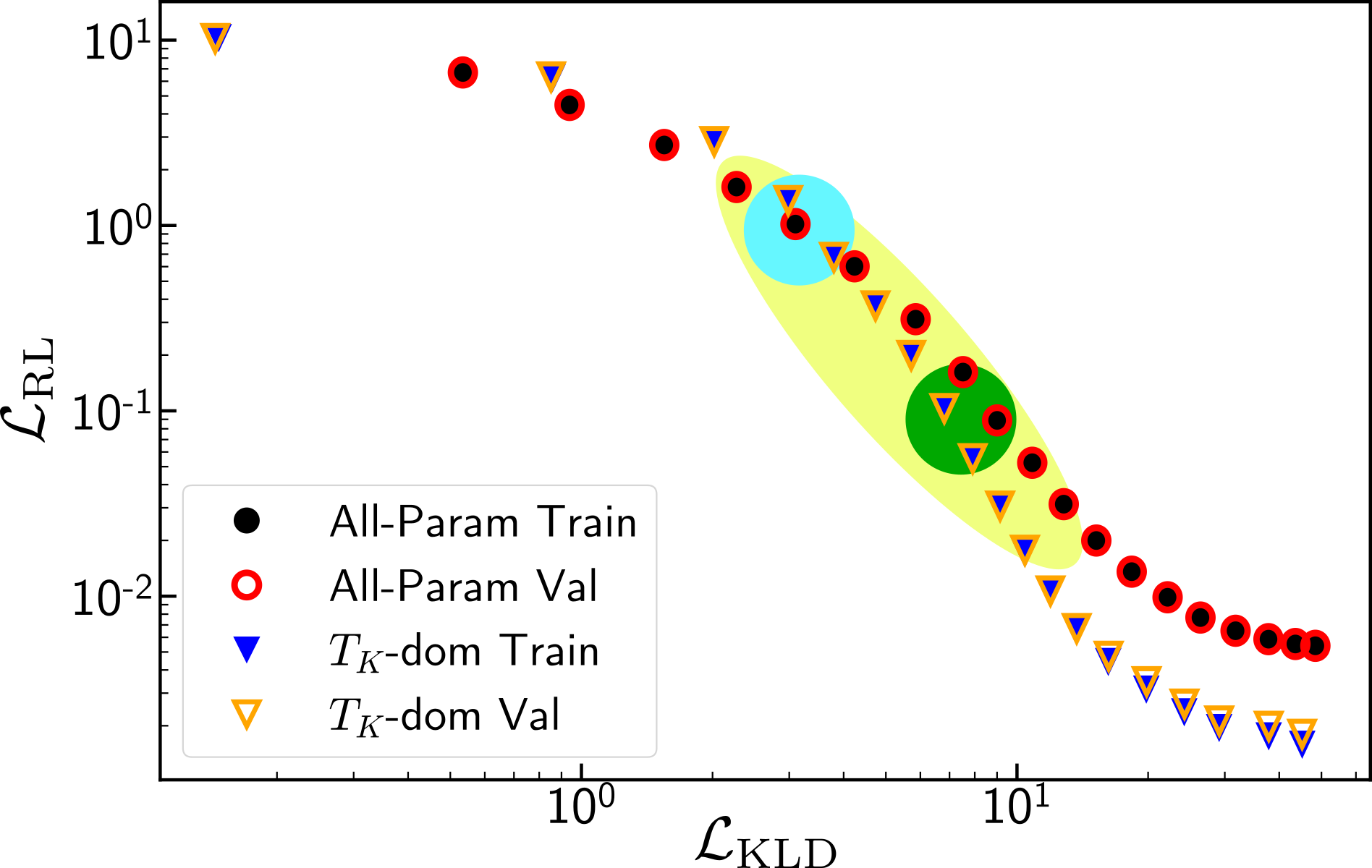
By scanning multiple models trained at various values, we find that a reasonable method for identifying critical VAE regions is to plot versus as in Fig. 2(a), but on a log-log scale as in Fig. A10. Notably, the shape of this curve is independent of an overall scaling of the data, which simply shifts the curve in log-log space. We note that the critical region appears as a clearly defined inflection point, which we can identify as a local optimum in the first derivative. To select our final models shown in the main text, we train multiple randomly-initialized VAEs with the same , and choose the model with the fewest active latent neurons and the simplest structure in latent space.
A.3 Machine Learning Implementation
We construct our neural networks using the PyTorch Paszke et al. (2019) deep learning library, and train them using standard minibatch training with the ADAM Kingma and Ba (2015) optimizer for a total of epochs. Every epoch, the training dataset is randomly partitioned into “minibatches” with batch_size = 1024 spectral functions. Model parameters are updated once per batch using gradients backpropagated from the error on the samples within the minibatch. Step sizes are adaptively computed within the ADAM algorithm, with an upper bound set by the learning rate (lr) hyperparameter. This lr, initially set to , is modified each epoch according to a cosine annealing schedule Loshchilov and Hutter (2017) as implemented by Pytorch’s CosineAnnealingLR. Between each fully connected layer of our network, we employ a batch normalization Ioffe and Szegedy (2015) layer to promote gradient backflow. Our code is made public at https://github.com/ColeMiles/SpectralVAE.

As mentioned in the main text, we anneal the regularization strength by ramping up from to the final value across the first fraction of the training epochs. This is heuristically found to improve the quality of trained VAEs Bowman et al. (2016), due to avoiding local minima where the model solely focuses on minimizing . The exact form of this ramping is not found to significantly affect results as long as it is done slowly enough, and we employ a ramp of the form with the current epoch number.
In Fig. A11(a), we show final reconstruction performance results for unregularized () VAEs as is varied. When the latent dimension size is large, we note a significant plateau in reconstruction performance. This plateau is already firmly established by , motivating our choice to set this as the latent size of our VAEs. We also note a “critical” latent , smaller than which reconstruction performance rapidly worsens. Interestingly, this is roughly and for the -dominated and full-parameter datasets respectively, corresponding to the number of free physical parameters in each case. This provides an alternate method to extract the critical dimension from that shown in the main text.
Once we turn on the regularization loss (i.e. ), this drives the learned latent features to become statistically independent. In the VAE literature, statistically independent features are referred to as “disentangled” Higgins et al. (2016); Mathieu et al. (2019). We define a heuristic metric of success towards this goal as the normalized sum of the off-diagonal elements of the covariance matrix. With being the standard covariance, we define normalized elements as:
| (10) |
and define a “disentangling” metric as , which becomes zero when all ’s are completely independent. In Fig. A11(b), we show that this metric rapidly decreases with increasing , demonstrating how the regularization pushes the latent ’s towards statistical independence.
Appendix B Alternate Views of Latent Space
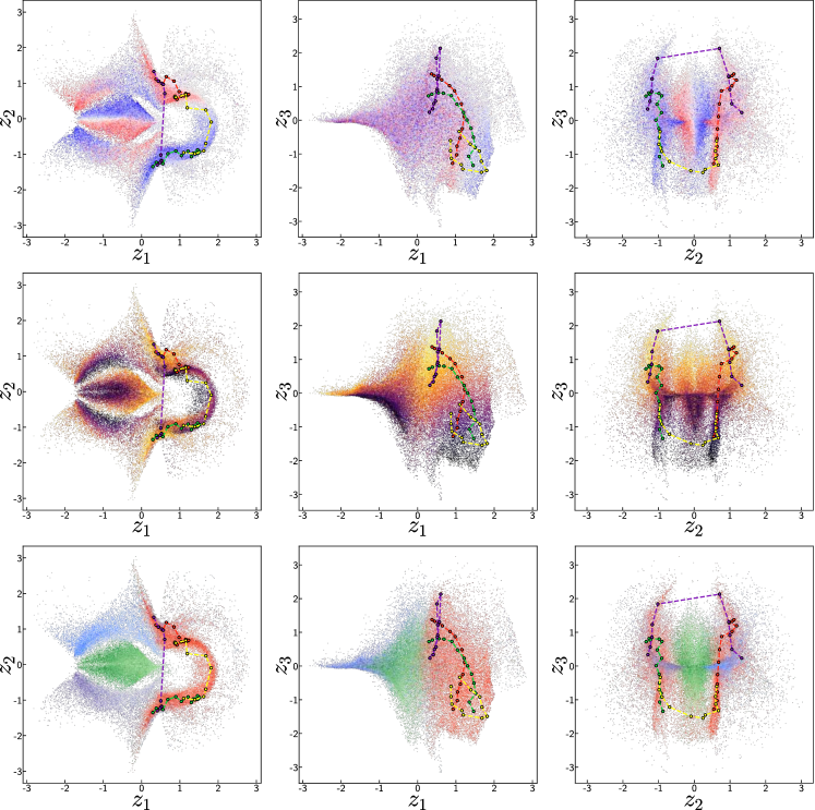
Here we offer the reader additional viewpoints into the VAE-learned latent spaces characterizing the full-parameter dataset. In particular, Fig. A12 shows multiple plane projections of the VAE presented in the main text (Fig. 6). Each column shows a different plane projection onto two of the active latents, while each row colors the points according to , or the dominant energy scale , with each colormap as in Fig. 6. A particular feature which is more evident here is the strong correlation between the latent and the smallest physical energy scale (second row).
Next, in Fig. A13 we show the learned latent spaces of two additional randomly initialized, independently trained VAEs at the same value of . Both of the models presented have a higher total loss than the VAE presented in the main text. However, they can be seen to have qualitatively similar (but lower-quality) structure in latent space. On rare occasions the learned structure will “twist” into an extra dimension, but these are easily identifiable by a large loss. In practice, due to the presence of multiple local minima in the loss function it is necessary to train multiple models and analyze the best-performing one.
Appendix C Comparison to linear dimensionality reduction
Since we do not make use of the generative aspects of VAEs in this work, their application here can be understood as an example in the broader class of “dimensionality reduction” or “representation learning” Bengio et al. (2013) techniques. All methods falling into this category attempt to find a low-dimensional parameterization of a collection of high-dimensional data. Due to their disentangling property, we find VAEs are particularly well suited for discovering independent, physically meaningful descriptors, but other dimensionality reduction techniques may also fit into our pipeline. To demonstrate this, we compare our results from the main text to the results of a linear dimensionality reduction approach provided by principal component analysis (PCA).
Principal component analysis is a simple, parameter-free technique for discovering the directions in a feature space which vary the most within a dataset. Thinking of each input spectral function as a -dimensional vector , PCA is done by simply diagonalizing the covariance matrix , with the expectations taken over the dataset. The resulting eigenvectors can be thought of as a rotated orthogonal basis of this vector space ordered such that the first basis vector points along the direction of greatest variance in the dataset (with its corresponding eigenvalue the variance), and then decreasing in variance for each subsequent vector. A dimensionality reduction can then be achieved by projecting the original data onto the first few of these principal component vectors.
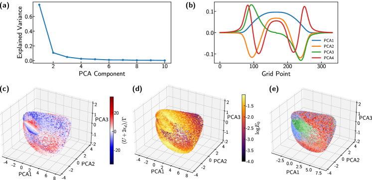
We show the results of applying PCA to the full-parameter dataset in Fig. A14. In Fig. A14(a), we show that a great fraction of the total variance of the data is captured by only a few principal components, four of which we plot in Fig. A14(b). We can see that the first of these components (blue) measures the broad central spectral weight, the second and fourth (orange, red) characterize the width of the central peak, and the third (green) characterizes some measure of asymmetry. We note that our dataset as a whole is very nearly symmetric about the central frequency – for every spectra in the dataset there exists another spectra which is approximately its mirror about the center. As a result, all of the principal components are either symmetric or antisymmetric about the center.
While these features are somewhat similar to those discovered by the VAE, the reduced space is obtained only from linear projections onto these curves. We find that this is sufficient to somewhat capture the particle-hole asymmetry and overall energy scale (Fig. A14(c,d)), but the separate energy scales are folded together in a somewhat complex way (Fig. A15). Evidently, some nonlinear transformations are needed to properly unfold this structure into one where all physically meaningful descriptors are naturally aligned with the new dimensions. A virtue of the VAE process is that we can arrive at a minimal set of such features, even capturing more complex features are shown in the following section.
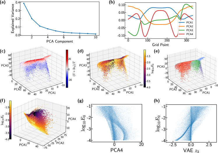
A typical method for applying PCA is to perform some amount of feature normalization as a preprocessing step. One standard scheme is to normalize the spectra such that each frequency is independently normalized to zero-mean and unit-variance across the dataset, i.e. . This normalization approach effectively emphasizes subtle details in the tails of , putting them on the same scale as other changes. In Fig. A14, we show the result of applying PCA to the full five-parameter dataset after this normalization has first been performed. We see in Fig. A14(b) that again the first and third components measure the broad central spectral weight and asymmetry respectively, while the the second and fourth (orange, red) now characterize the amount of weight in the tails compared to the center.
Surprisingly, this new normalization process has made various energy scales separate out far more cleanly. In particular, the various dominating energy scales are now visible as distinct lobes in Fig. A15(e). Additionally, the smallest physical energy now appears correlated with PCA4 as shown in Fig. A15(f,g), though not quite as sharply as the correlation with the VAE-discovered latent (Fig. A15(h)). We remark that although the VAE did not have the benefit of this human-inspired normalization scheme, it was nonetheless able to discover a set of features that directly correlates with known physics.
Appendix D Latent Traversals of Weaker-Regularization Models
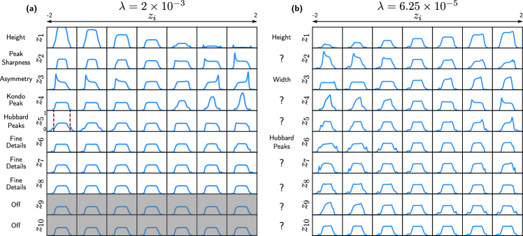
In the main text, for simplicity of presentation we examined VAEs trained with a rather strong regularization of which were found to smoothly capture high-level information about our dataset. However, as a consequence of this strong regularization our models miss smaller features such as details of the Hubbard side peaks in the spectral functions. Indeed, it is a well-known phenomena that VAE reconstructions tend to appear “blurred” compared to the original input Higgins et al. (2017). In Fig. A16, we examine VAEs trained with weaker regularization strengths by scanning each latent dimension while keeping all others at zero. We find that at intermediate regularization we can capture additional meaningful features in the dataset beyond those presented in the main text, demonstrating that we are not limited by the learning capacity of our VAE.
For in Fig. A16(a), we find that two latent variables are completely inactive, and two additional variables () barely affect the reconstruction. For the remaining active neurons, we can still (partially) assign meaningful descriptors even at this weaker regularization. Additionally, we can tell from our disentangling metric (Fig. A11(b)) that these variables are more correlated with each other than at . In particular, these additional active latents appear to capture fine details about the development of the Hubbard side peaks in the spectra.
At even smaller in Fig. A16(b), we see that all latent variables seem to affect the reconstruction in at least a minor way. Additionally, we see that it is difficult to separate the latent variables into particular physical effects on the reconstruction, as multiple variables can be seen to produce similar changes on the resulting spectral function.
References
- Damascelli et al. (2003) A. Damascelli, Z. Hussain, and Z.-X. Shen, Rev. Mod. Phys. 75, 473 (2003).
- Valla et al. (1999) T. Valla, A. V. Fedorov, P. D. Johnson, and S. L. Hulbert, Phys. Rev. Lett. 83, 2085 (1999).
- Dean et al. (2016) M. P. M. Dean, Y. Cao, X. Liu, S. Wall, D. Zhu, R. Mankowsky, V. Thampy, X. M. Chen, J. G. Vale, D. Casa, J. Kim, A. H. Said, P. Juhas, R. Alonso-Mori, J. M. Glownia, A. Robert, J. Robinson, M. Sikorski, S. Song, M. Kozina, H. Lemke, L. Patthey, S. Owada, T. Katayama, M. Yabashi, Y. Tanaka, T. Togashi, J. Liu, C. Rayan Serrao, B. J. Kim, L. Huber, C.-L. Chang, D. F. McMorrow, M. Först, and J. P. Hill, Nature Materials 15, 601 (2016).
- Mahan (2013) G. D. Mahan, Many-particle Physics (Springer Science & Business Media, 2013).
- Bengio et al. (2013) Y. Bengio, A. Courville, and P. Vincent, IEEE Transactions on Pattern Analysis and Machine Intelligence 35, 1798 (2013).
- Tschannen et al. (2018) M. Tschannen, O. Bachem, and M. Lucic, “Recent Advances in Autoencoder-Based Representation Learning,” (2018), arXiv:1812.05069 [cs.LG] .
- Kingma and Welling (2014) D. P. Kingma and M. Welling, in 2nd International Conference on Learning Representations, ICLR 2014, Banff, AB, Canada, April 14-16, 2014, Conference Track Proceedings, edited by Y. Bengio and Y. LeCun (2014).
- Doersch (2021) C. Doersch, “Tutorial on variational autoencoders,” (2021), arXiv:1606.05908 [stat.ML] .
- Higgins et al. (2017) I. Higgins, L. Matthey, A. Pal, C. Burgess, X. Glorot, M. Botvinick, S. Mohamed, and A. Lerchner, in 5th International Conference on Learning Representations, ICLR 2017, Toulon, France, April 24-26, 2017, Conference Track Proceedings (OpenReview.net, 2017).
- Martínez-Palomera et al. (2020) J. Martínez-Palomera, J. S. Bloom, and E. S. Abrahams, “Deep generative modeling of periodic variable stars using physical parameters,” (2020), arXiv:2005.07773 [astro-ph.IM] .
- Otten et al. (2021) S. Otten, S. Caron, W. de Swart, M. van Beekveld, L. Hendriks, C. van Leeuwen, D. Podareanu, R. Ruiz de Austri, and R. Verheyen, Nature Communications 12, 2985 (2021).
- Farina et al. (2020) M. Farina, Y. Nakai, and D. Shih, Phys. Rev. D 101, 075021 (2020).
- Cerri et al. (2019) O. Cerri, T. Q. Nguyen, M. Pierini, M. Spiropulu, and J.-R. Vlimant, Journal of High Energy Physics 2019, 36 (2019).
- Wetzel (2017) S. J. Wetzel, Phys. Rev. E 96, 022140 (2017).
- Kottmann et al. (2020) K. Kottmann, P. Huembeli, M. Lewenstein, and A. Acín, Phys. Rev. Lett. 125, 170603 (2020).
- Samarakoon et al. (2020) A. M. Samarakoon, K. Barros, Y. W. Li, M. Eisenbach, Q. Zhang, F. Ye, V. Sharma, Z. L. Dun, H. Zhou, S. A. Grigera, C. D. Batista, and D. A. Tennant, Nature Communications 11, 892 (2020).
- Routh et al. (2021) P. K. Routh, Y. Liu, N. Marcella, B. Kozinsky, and A. I. Frenkel, The Journal of Physical Chemistry Letters 12, 2086 (2021).
- Lu et al. (2020) P. Y. Lu, S. Kim, and M. Soljačić, Phys. Rev. X 10, 031056 (2020).
- Kalinin et al. (2021) S. V. Kalinin, O. Dyck, S. Jesse, and M. Ziatdinov, Science Advances 7, eabd5084 (2021).
- Schmidt and Lipson (2009) M. Schmidt and H. Lipson, Science 324, 81 (2009).
- Bongard and Lipson (2007) J. Bongard and H. Lipson, Proceedings of the National Academy of Sciences 104, 9943 (2007).
- Anderson (1961) P. W. Anderson, Phys. Rev. 124, 41 (1961).
- Kondo (1964) J. Kondo, Progress of Theoretical Physics 32, 37 (1964).
- Wilson (1975) K. G. Wilson, Rev. Mod. Phys. 47, 773 (1975).
- Bulla et al. (2008) R. Bulla, T. A. Costi, and T. Pruschke, Rev. Mod. Phys. 80, 395 (2008).
- Weichselbaum and von Delft (2007) A. Weichselbaum and J. von Delft, Phys. Rev. Lett. 99, 076402 (2007).
- Weichselbaum (2012) A. Weichselbaum, Phys. Rev. B 86, 245124 (2012), arXiv:1209.2062 .
- Sturm et al. (2021) E. J. Sturm, M. R. Carbone, D. Lu, A. Weichselbaum, and R. M. Konik, Phys. Rev. B 103, 245118 (2021).
- Haldane (1978) F. D. M. Haldane, Phys. Rev. Lett. 40, 416 (1978).
- Tsvelick and Wiegmann (1983) A. Tsvelick and P. Wiegmann, Advances in Physics 32, 453 (1983).
- Note (1) This cutoff in was heuristically chosen to both minimize the effects of while keeping the dataset roughly the same size as our full-parameter dataset.
- Higgins et al. (2016) I. Higgins, L. Matthey, X. Glorot, A. Pal, B. Uria, C. Blundell, S. Mohamed, and A. Lerchner, “Early visual concept learning with unsupervised deep learning,” (2016), arXiv:1606.05579 [stat.ML] .
- Bowman et al. (2016) S. R. Bowman, L. Vilnis, O. Vinyals, A. Dai, R. Jozefowicz, and S. Bengio, in Proceedings of The 20th SIGNLL Conference on Computational Natural Language Learning (Association for Computational Linguistics, Berlin, Germany, 2016) pp. 10–21.
- Kingma and Ba (2015) D. P. Kingma and J. Ba, in 3rd International Conference on Learning Representations, ICLR 2015, San Diego, CA, USA, May 7-9, 2015, Conference Track Proceedings, edited by Y. Bengio and Y. LeCun (2015).
- Note (2) We observe that the variance in final losses between trained models is negligible for the purposes of constructing the loss curves in Fig. 2(a). However, due to multiple local minima, at some there is occasionally active latent in the final model.
- Cranmer et al. (2020) M. Cranmer, A. Sanchez Gonzalez, P. Battaglia, R. Xu, K. Cranmer, D. Spergel, and S. Ho, in Advances in Neural Information Processing Systems, Vol. 33, edited by H. Larochelle, M. Ranzato, R. Hadsell, M. F. Balcan, and H. Lin (Curran Associates, Inc., 2020) pp. 17429–17442.
- Stephens (2015) T. Stephens, “Gplearn,” https://github.com/trevorstephens/gplearn (2015).
- Pal and Wang (1996) S. K. Pal and P. P. Wang, eds., Genetic Algorithms for Pattern Recognition (CRC Press, Boca Raton, 1996).
- Deb et al. (2002) K. Deb, A. Pratap, S. Agarwal, and T. Meyarivan, IEEE Transactions on Evolutionary Computation 6, 182 (2002).
- Mathieu et al. (2019) E. Mathieu, T. Rainforth, N. Siddharth, and Y. W. Teh, in Proceedings of the 36th International Conference on Machine Learning, Proceedings of Machine Learning Research, Vol. 97, edited by K. Chaudhuri and R. Salakhutdinov (PMLR, 2019) pp. 4402–4412.
- Petersen et al. (2021) B. K. Petersen, M. L. Larma, T. N. Mundhenk, C. P. Santiago, S. K. Kim, and J. T. Kim, in International Conference on Learning Representations (2021).
- Udrescu and Tegmark (2020) S.-M. Udrescu and M. Tegmark, Science Advances 6 (2020), 10.1126/sciadv.aay2631.
- Reinbold et al. (2021) P. A. K. Reinbold, L. M. Kageorge, M. F. Schatz, and R. O. Grigoriev, Nature Communications 12, 3219 (2021).
- Miles et al. (2021) C. Miles, M. R. Carbone, E. J. Sturm, D. Lu, A. Weichselbaum, K. Barros, and R. M. Konik, “Dataset used in ”Machine-learning Kondo physics using variational autoencoders”,” (2021).
- Paszke et al. (2019) A. Paszke, S. Gross, F. Massa, A. Lerer, J. Bradbury, G. Chanan, T. Killeen, Z. Lin, N. Gimelshein, L. Antiga, A. Desmaison, A. Kopf, E. Yang, Z. DeVito, M. Raison, A. Tejani, S. Chilamkurthy, B. Steiner, L. Fang, J. Bai, and S. Chintala, in Advances in Neural Information Processing Systems 32 (Curran Associates, Inc., 2019) pp. 8024–8035.
- Loshchilov and Hutter (2017) I. Loshchilov and F. Hutter, in 5th International Conference on Learning Representations, ICLR 2017, Toulon, France, April 24-26, 2017, Conference Track Proceedings (OpenReview.net, 2017).
- Ioffe and Szegedy (2015) S. Ioffe and C. Szegedy, in Proceedings of the 32nd International Conference on Machine Learning, ICML 2015, Lille, France, 6-11 July 2015, JMLR Workshop and Conference Proceedings, Vol. 37, edited by F. R. Bach and D. M. Blei (JMLR.org, 2015) pp. 448–456.