Noise-Aware Video Saliency Prediction

Abstract

We tackle the problem of predicting saliency maps for videos of dynamic scenes. We note that the accuracy of the maps reconstructed from the gaze data of a fixed number of observers varies with the frame, as it depends on the content of the scene. This issue is particularly pressing when a limited number of observers are available. In such cases, directly minimizing the discrepancy between the predicted and measured saliency maps, as traditional deep-learning methods do, results in overfitting to the noisy data. We propose a noise-aware training (NAT) paradigm that quantifies and accounts for the uncertainty arising from frame-specific gaze data inaccuracy. We show that NAT is especially advantageous when limited training data is available, with experiments across different models, loss functions, and datasets. We also introduce a video game-based saliency dataset, with rich temporal semantics, and multiple gaze attractors per frame. The dataset and source code are available at https://github.com/NVlabs/NAT-saliency.

1 Introduction

Humans can perceive high-frequency details only within a small solid angle, and thus, analyze scenes by directing their gaze to the relevant parts [Geisler and Perry(1998), Deza and Eckstein(2016)]. Predicting a distribution of gaze locations (i.e, a saliency map) for a visual stimulus has widespread applications such as image or video compression [Baek et al.(2020)Baek, Kang, and Ryoo] and foveated rendering [Kim et al.(2019)Kim, Jeong, Stengel, Akşit, Albert, Boudaoud, Greer, Kim, Lopes, Majercik, Shirley, Spjut, McGuire, and Luebke, Kaplanyan et al.(2019)Kaplanyan, Sochenov, Leimkühler, Okunev, Goodall, and Rufo], among others. This has inspired an active area of research – visual saliency prediction. Early methods focused on low- or mid-level visual features [Itti et al.(1998)Itti, Koch, and Niebur, Itti and Koch(2000), Koch and Ullman(1987)], and recent methods leverage high-level priors through deep learning (DL) for saliency prediction and related tasks such as salient object detection [Huang et al.(2015)Huang, Shen, Boix, and Zhao, Kümmerer et al.(2017)Kümmerer, Wallis, Gatys, and Bethge, Kümmerer et al.(2014)Kümmerer, Theis, and Bethge, Pan et al.(2017)Pan, Ferrer, McGuinness, O’Connor, Torres, Sayrol, and Giro-i Nieto, Wang and Shen(2017), Jia and Bruce(2020), Kruthiventi et al.(2017)Kruthiventi, Ayush, and Babu, Liu and Han(2018), Liu et al.(2015)Liu, Han, Zhang, Wen, and Liu, Gao et al.(2020)Gao, Zhao, Liu, and Wang, Zhang et al.(2020b)Zhang, Han, Liu, , and Shao, Zhang et al.(2020a)Zhang, Xie, and Barnes, Liu et al.(2021)Liu, Zhang, Wan, Han, and Shao].

Figure 1: Motivation for noise-aware training (NAT). Frames from a video (DIEM [Mital et al.(2011)Mital, Smith, Hill, and Henderson] dataset) are shown with an overlay of the saliency maps reconstructed from the gaze data of $95$ observers. The level of gaze consistency across observers varies with frame content, leading to different asymptotic values and convergence rates of the per-frame inter-observer consistency (IOC) curves. Consequently, the accuracy of the saliency maps reconstructed from gaze data varies across frames – especially when a limited number of observers (say, $5$ observers) are available. This impedes traditional training that directly minimizes the discrepancy between predicted and measured maps. We introduce NAT to address this.

Given the improved accessibility of eye trackers [Valliappan et al.(2020)Valliappan, Dai, Steinberg, He, Rogers, Ramachandran, Xu, Shojaeizadeh, Guo, Kohlhoff, et al.], datasets for saliency prediction are captured by recording gaze locations of observers viewing an image or a video. These gaze locations are then used to estimate a per-frame/image saliency map. Generally speaking, the quality of the reconstructed saliency maps increases with the number of gaze samples. However, two factors make it particularly challenging to reconstruct high-quality maps for videos. First, since a single observer contributes only a few (typically one [Mital et al.(2011)Mital, Smith, Hill, and Henderson]) gaze locations per video frame, more observers are needed to capture sufficient per-frame gaze data for videos as compared to images (e.g, the CAT2000 dataset has on average ${\sim}333$ fixations per image from $24$ observers [Borji and Itti(2015)], while LEDOV has ${\sim}32$ fixations per video frame from $32$ observers [Jiang et al.(2021)Jiang, Xu, Wang, and Sigal]). Therefore, the cost associated with the creation of truly large-scale datasets with tens of thousands of videos can be prohibitively high. Second, for videos of dynamic scenes, it is hard to guarantee high accuracy of the reconstructed saliency maps across all frames from the gaze data of a fixed number of observers. This is because the gaze behavior consistency across observers depends on the scene content [Wilming et al.(2011)Wilming, Betz, Kietzmann, and König]: scenes that elicit a high consistency would require fewer observers to reconstruct accurate saliency maps than those for which the inter-observer consistency (IOC) in gaze behavior is low.

Fig. 1 shows $3$ frames from a DIEM video [Mital et al.(2011)Mital, Smith, Hill, and Henderson] with 95-observer saliency map overlays and the per-frame IOC as a function of the number of observers used to reconstruct the saliency map [Kümmerer et al.(2015)Kümmerer, Wallis, and Bethge, Wilming et al.(2011)Wilming, Betz, Kietzmann, and König, Jiang et al.(2021)Jiang, Xu, Wang, and Sigal]. A converged IOC curve indicates that additional observers do not add new information to the reconstructed saliency map and the captured number of observers (e.g, $95$ in Fig. 1) are sufficient for accurate estimation of saliency [Jiang et al.(2021)Jiang, Xu, Wang, and Sigal, Judd et al.(2012)Judd, Durand, and Torralba]. As is clear from these plots, when the number of available observers is small, the IOC curve differs from its asymptotic value by a varying amount for each frame. This leads to varying per-frame accuracy of the saliency map reconstructed from few observers. In such cases, traditional training methods, which minimize the discrepancy between the predicted and measured saliency, can lead to overfitting to the inaccurate saliency maps in the training dataset.

We address these issues by proposing a Noise-Aware Training (NAT) paradigm: we interpret the discrepancy $d$ between the measured and predicted saliency maps as a random variable, and train the saliency predictor through likelihood maximization. We show that NAT avoids overfitting to incomplete or inaccurate saliency maps, weighs training frames based on their reliability, and yields consistent improvement over traditional training, for different datasets, deep neural networks (DNN), and training discrepancies, especially when few observers or frames are available for training. Therefore, NAT ushers in the possibility of designing larger-scale video-saliency datasets with fewer observers per video, since it learns high-quality models with less training data.

Although existing datasets have been vital to advance video saliency research [Jiang et al.(2021)Jiang, Xu, Wang, and Sigal, Mital et al.(2011)Mital, Smith, Hill, and Henderson], a significant portion of these datasets consists of almost-static content, as observed recently by Tangemann et al. [Tangemann et al.(2020)Tangemann, Kümmerer, Wallis, and Bethge]. Using these datasets for training and evaluation therefore makes it difficult to assess how saliency prediction methods fare on aspects specific to videos, such as predicting saliency on temporally-evolving content. Consequently, even an image-based saliency predictor can provide good results for existing video saliency datasets [Tangemann et al.(2020)Tangemann, Kümmerer, Wallis, and Bethge]. As a step towards designing datasets with dynamic content, we introduce the Fortnite Gaze Estimation Dataset (ForGED), that contains clips from game-play videos of Fortnite, a third-person-shooter game amassing hundreds of million of players worldwide. With ForGED, we contribute a novel dataset with unique characteristics such as: fast temporal dynamics, semantically-evolving content, multiple attractors of attention, and a new gaming context.

2 Related work

Saliency prediction methods.

In recent years, DL-based approaches have remarkably advanced video saliency prediction [Borji(2019)]. Existing works include (i) 3D CNN architectures that observe a short sub-sequence of frames [Jain et al.(2021)Jain, Yarlagadda, Jyoti, Karthik, Subramanian, and Gandhi, Bellitto et al.(2020)Bellitto, Salanitri, Palazzo, Rundo, Giordano, and Spampinato, Min and Corso(2019)]; (ii) architectures that parse one frame at a time but maintain information about past frames in feature maps (e.g, simple temporal accumulation or LSTMs [Linardos et al.(2019)Linardos, Mohedano, Nieto, O’Connor, Giro-i Nieto, and McGuinness, Wang et al.(2018)Wang, Shen, Guo, Cheng, and Borji, Gorji and Clark(2018), Wu et al.(2020)Wu, Wu, Zhang, Ju, and Wang, Droste et al.(2020)Droste, Jiao, and Noble]); or (iii) a combination of both [Bazzani et al.(2016)Bazzani, Larochelle, and Torresani]. Some methods also decouple spatial and temporal saliency through specific features, such as “object-ness” and motion in a frame [Jiang et al.(2018)Jiang, Xu, Liu, Qiao, and Wang, Jiang et al.(2021)Jiang, Xu, Wang, and Sigal, Bak et al.(2017)Bak, Kocak, Erdem, and Erdem], adopt vision transformers [Liu et al.(2021)Liu, Zhang, Wan, Han, and Shao], or predict a compact spatial representations such as a GMM [Reddy et al.(2020)Reddy, Jain, Yarlagadda, and Gandhi]. Overall, existing works largely focus on improving model architectures, output representations [Reddy et al.(2020)Reddy, Jain, Yarlagadda, and Gandhi], and training procedures. In contrast, our NAT paradigm is broadly applicable across all these categories and it only modifies the loss function to account for the level of reliability of the measured saliency maps. We demonstrate the model-agnostic applicability of NAT through experiments on representative DNN architectures – we use ViNET [Jain et al.(2021)Jain, Yarlagadda, Jyoti, Karthik, Subramanian, and Gandhi] (2021 state-of-the-art that uses 3D CNN), TASED-Net [Min and Corso(2019)] (a 3D CNN-based model), and SalEMA [Linardos et al.(2019)Linardos, Mohedano, Nieto, O’Connor, Giro-i Nieto, and McGuinness].

Metrics and measures of uncertainty for saliency.

Popular metrics for training and evaluating saliency models include density-based functions (Kullback-Leibler divergence, KLD, correlation coefficient, CC, similarity, SIM [Swain and Ballard(1991)]), and fixation-based functions (area under the ROC curve, AUC [Bylinskii et al.(2018)Bylinskii, Judd, Oliva, Torralba, and Durand, Bylinskii et al.(2015)Bylinskii, Judd, Borji, Itti, Durand, Oliva, and Torralba], normalized scanpath saliency, NSS [Peters et al.(2005)Peters, Iyer, Itti, and Koch, Riche et al.(2013)Riche, Duvinage, Mancas, Gosselin, and Dutoit, Bylinskii et al.(2018)Bylinskii, Judd, Oliva, Torralba, and Durand]). Fixation-based metrics evaluate saliency at the captured gaze locations, without reconstructing the entire map. We observed that when few locations on a small training set are available, models that directly optimize either type of function show suboptimal performance.

The adoption of correction terms on a incomplete probability distributions has been explored in population satistics [Chao and Shen(2003), Holste et al.(1998)Holste, Grosse, and Herzel]. Adapting these concepts to gaze data is possible at low spatial resolutions [Wilming et al.(2011)Wilming, Betz, Kietzmann, and König]. However, at full resolution, gaze data tends to be too sparse to collect sufficient statistics in each pixel. IOC curves are also used to estimate the level of completeness of saliency maps [Jiang et al.(2021)Jiang, Xu, Wang, and Sigal], and the upper bounds on the performance of a saliency predictor  [Wilming et al.(2011)Wilming, Betz, Kietzmann, and König, Judd et al.(2012)Judd, Durand, and Torralba, Le Meur and Baccino(2013), Kümmerer et al.(2015)Kümmerer, Wallis, and Bethge]. Such approaches provide an insight on level of accuracy and uncertainty in saliency maps, but depend on the availability of sufficient observers to estimate the full curves. In contrast, NAT is designed specifically for limited-data setting.

Video saliency datasets.

Some datasets capture video saliency for specific content (like sports [Rodriguez et al.(2008)Rodriguez, Ahmed, and Shah], movies [Vig et al.(2012)Vig, Dorr, and Cox], faces [Liu et al.(2017)Liu, Zhang, Xu, and He]), while others (like DHF1K [Wang et al.(2018)Wang, Shen, Guo, Cheng, and Borji], LEDOV [Jiang et al.(2018)Jiang, Xu, Liu, Qiao, and Wang], and DIEM [Mital et al.(2011)Mital, Smith, Hill, and Henderson]) do for everyday scenes [Borji(2019)]. We perform our experimental analysis using two of the largest datasets, DIEM and LEDOV, which also provide high-quality gaze annotations, and, more importantly, access to per-observer gaze data – a feature that is not available in the most popular DHF1K dataset, among other artifacts [Tangemann et al.(2020)Tangemann, Kümmerer, Wallis, and Bethge].

Videos with dynamic content are key to capturing and assessing video-specific saliency. However, existing datasets contain mostly-static content, which can be explained by image-based models [Tangemann et al.(2020)Tangemann, Kümmerer, Wallis, and Bethge]. Existing datasets with videos of highly-dynamic content are either constrained in visual content variety and real-time gaze capture (e.g, Atari-Head dataset [Zhang et al.(2019)Zhang, Walshe, Liu, Guan, Muller, Whritner, Zhang, Hayhoe, and Ballard]), or capture gaze data from only a single subject (such as a game player [Borji and Itti(2012)], or a driver [Alletto et al.(2016)Alletto, Palazzi, Solera, Calderara, and Cucchiara]), limiting the accuracy of test-time evaluations. We therefore turn to game-play videos of Fortnite, with its rich temporal dynamics, to further evaluate video-specific saliency. ForGED features videos from Fortnite with gaze data from up to $21$ observers per video frame, enabling an effective benchmark for training and evaluating video-specific saliency.

3 Noise-Aware Training (NAT)

Figure 2: Overview of NAT. For an input image, a saliency map is approximated from measured gaze data. This can result in a noisy/incomplete version of the GT saliency – especially when limited gaze data is available. Instead of training a DNN by directly minimizing the discrepancy, $d$, between the measured and predicted saliency (traditional training), with NAT we first estimate a distribution for $d$, $p(d)$, that quantifies the uncertainty in $d$ due to the inaccuracies in the measured saliency maps. We then train the DNN to optimize the likelihood of $d$.

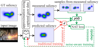
The accuracy of the saliency maps in videos varies with frame content, especially when limited gaze data is available. The inaccuracy in the saliency maps can stem from errors in gaze measurements, such as inaccurate localization of Purkinje reflections or calibration issues in gaze tracker [Feit et al.(2017)Feit, Williams, Toledo, Paradiso, Kulkarni, Kane, and Morris] – we term these measurement noise. Using an insufficient number of observers to estimate the probabilities in different sub-regions of the saliency map is another source of noise, which we term incomplete sampling. While the measurement noise can be partially alleviated with techniques such as temporal filtering [Chartier and Renaud(2008)], the best way to overcome both sources of noise is to capture sufficient data. Since this can be impractical, we now discuss our proposed strategy to effectively train a DNN for saliency prediction, accounting for the noise level in a measured saliency map (Fig. 2).

Let $x_{i}$ be the probability distribution of the ground-truth saliency map for the $i^{th}$ frame, reconstructed from sufficient gaze data (e.g, when the IOC curve is close to its asymptotic value). The traditional approach to train a saliency predictor (abbreviated as TT : traditional training) optimizes:

$$J^{\text{ideal}}=\sum\nolimits_{i}d(\hat{x}_{i},x_{i}),$$ (1)

where $\hat{x}_{i}$ is the predicted saliency map, and $d(\cdot,\cdot)$ is a discrepancy measure such as KLD, CC, NSS, or a mix of these. Since reconstructing an accurate $x_{i}$ is challenging, the existing methods instead end up optimizing:

$$J^{\text{real}}=\sum\nolimits_{i}d(\hat{x}_{i},\tilde{x}_{i}),$$ (2)

where $\tilde{x}_{i}$ is an approximation of the unobservable $x_{i}$. We adopt the standard practice to estimate $\tilde{x}_{i}$ from captured gaze data [Jiang et al.(2021)Jiang, Xu, Wang, and Sigal, Ehinger et al.(2009)Ehinger, Hidalgo-Sotelo, Torralba, and Oliva, Wilming et al.(2011)Wilming, Betz, Kietzmann, and König]: spatial locations are sampled from $x_{i}$ during gaze acquisition, followed by blurring with a Gaussian kernel and normalization to obtain the probability density function (pdf) $\tilde{x}_{i}$. This can also be seen as a Gaussian Mixture Model with equal-variance components at measured gaze locations. Let us denote this process of sampling spatial locations and reconstructing a pdf (“SR”) as:

$$\tilde{x}_{i}\ =\ SR(x_{i}\ ;\ N),$$ (3)

where $N$ is the number of spatial locations sampled from $x_{i}$ via gaze data capture. For videos, $N$ is equivalently the number of observers.

Given that $\tilde{x}_{i}$ can be prone to inaccuracies/noise, minimizing $J^{\text{real}}$ during training can lead to noise overfitting and suboptimal convergence (see Supplementary Sec. 8). Instead of directly minimizing $d(\hat{x}_{i},\tilde{x}_{i})$, our approach models the uncertainty in $d(x_{i},\tilde{x}_{i})$ due to the noise in $\tilde{x}_{i}$. We first estimate a probability density function for $d(\hat{x}_{i},\tilde{x}_{i})$, denoted by $p[d(x_{i},\tilde{x}_{i})]$, and then train the DNN for saliency prediction by maximizing the likelihood of $d(x_{i},\tilde{x}_{i})$.

We interpret $d(x_{i},\tilde{x}_{i})$ as Gaussian random variable with statistics $\operatorname{\mathbb{E}}[d(x_{i},\tilde{x}_{i})]$, $\text{Var}[d(x_{i},\tilde{x}_{i})]$. We first consider an ideal case where $x_{i}$ is available and therefore we can compute these statistics by sampling and reconstructing several realizations of $\tilde{x}_{i}$ from $x_{i}$ (Eq. 3; no gaze data acquisition needed), and then computing sample mean $\operatorname{\mathbb{E}}[d(x_{i},\tilde{x}_{i})]$ and variance $\text{Var}[d(x_{i},\tilde{x}_{i})]$. The value of these statistics depends on the number of available gaze locations $N$ used to reconstruct $\tilde{x}_{i}$ and on the complexity of $x_{i}$. For example, when $x_{i}$ consists of a simple, unimodal distribution – e.g, when only one location in a frame catches the attention of all the observers – a small $N$ is sufficient to bring $\tilde{x}_{i}$ close to $x_{i}$, which leads to low $\operatorname{\mathbb{E}}[d(x_{i},\tilde{x}_{i})]$ and $\text{Var}[d(x_{i},\tilde{x}_{i})]$ values. Alternatively, for a complex multimodal $x_{i}$, a larger $N$ is required for $\tilde{x}_{i}$ to converge to $x_{i}$ and consequently, $\operatorname{\mathbb{E}}[d(x_{i},\tilde{x}_{i})]$ and $\text{Var}[d(x_{i},\tilde{x}_{i})]$ are large when $N$ is small (more discussion on this in Supplementary, Sec. 2).

Our NAT cost function is then defined as the following negative log likelihood:

$$J_{\text{NAT}}=-\text{ln}\prod\nolimits_{i}p[d(\hat{x}_{i},\tilde{x}_{i})]=-\sum\nolimits_{i}\text{ln}\{p[d(\hat{x}_{i},\tilde{x}_{i})]\},$$ (4)

that enables us to account for the presence of noise in the training data, for any choice of $d$. If $\operatorname{\mathbb{E}}[d(x_{i},\tilde{x}_{i})]$ and $\text{Var}[d(x_{i},\tilde{x}_{i})]$ are known, and assuming that $d(x_{i},\tilde{x}_{i})$ is a Gaussian random variable, we can simplify Eq. 4 (see Supplementary, Sec. 1) to get:

$$J_{\text{NAT}}^{\text{ideal}}=\sum\nolimits_{i}{\{d(\hat{x}_{i},\tilde{x}_{i})-\operatorname{\mathbb{E}}[d(x_{i},\tilde{x}_{i})]\}^{2}}/{\text{Var}[d(x_{i},\tilde{x}_{i})]}.$$ (5)

We note that $J_{\text{NAT}}^{\text{ideal}}$ penalizes $\hat{x}_{i}$ that are far from $\tilde{x}_{i}$, as in the traditional case. However, it also ensures that $\hat{x}_{i}$ is not predicted too close to the noisy $\tilde{x}_{i}$, which helps prevent noise overfitting (similar to discrepancy principles applied in image denoising [Bertero et al.(2010)Bertero, Boccacci, Talenti, Zanella, and Zanni, Frosio and Kautz(2019)]). The penalization is inversely proportional to $\text{Var}[d(x_{i},\tilde{x}_{i})]$, i.e, it is strong for frames where $\tilde{x_{i}}$ is a good approximation of $x_{i}$. In contrast, $\operatorname{\mathbb{E}}[d(x_{i},\tilde{x}_{i})]$ and $\text{Var}[d(x_{i},\tilde{x}_{i})]$ are large for multimodal, sparse $\tilde{x}_{i}$ containing gaze data from only a few observers, since in such cases, $\tilde{x_{i}}$ is not a good approximation of $x_{i}$. This prevents the NAT formulation from overfitting to such uncertain $\tilde{x_{i}}$, by weakly penalizing the errors in $\hat{x}_{i}$ when compared to $\tilde{x}_{i}$.

However, Eq. 5 cannot be implemented in practice, as $x_{i}$ (and consequently $\operatorname{\mathbb{E}}[d(x_{i},\tilde{x}_{i})]$ and $\text{Var}[d(x_{i},\tilde{x}_{i})]$) is unknown. We only have access to $\tilde{x}_{i}$, a noisy realization of $x_{i}$. We therefore turn to approximating the statistics of $d(x_{i},\tilde{x}_{i})$ as:

$$\operatorname{\mathbb{E}}[d(x_{i},\tilde{x}_{i})]\approx\operatorname{\mathbb{E}}[d(\tilde{x}_{i},\tilde{\tilde{x}}_{i})],\;\text{Var}[d(x_{i},\tilde{x}_{i})]\approx\text{Var}[d(\tilde{x}_{i},\tilde{\tilde{x}}_{i})].$$ (6)

Here, $\tilde{\tilde{x_{i}}}\ =\ SR(\tilde{x_{i}}\ ;\ N)$ is the pdf obtained by sampling N spatial locations from $\tilde{x}_{i}$, followed by blurring ($N$ is also the number of gaze fixations sampled from $x_{i}$ by real observers). The difference between how $\tilde{x_{i}}$ is reconstructed from $x_{i}$ and $\tilde{\tilde{x_{i}}}$ from $\tilde{x_{i}}$ is in the manner of obtaining the $N$ spatial locations: the $N$ spatial locations used to reconstruct $\tilde{x}$ are obtained from human gaze when viewing the $i^{th}$ frame; while for reconstructing $\tilde{\tilde{x_{i}}}$, $N$ spatial locations are sampled from the pdf $\tilde{x_{i}}$. Multiple realizations of $\tilde{\tilde{x}}_{i}$ are then used to estimate $\operatorname{\mathbb{E}}[d(\tilde{x}_{i},\tilde{\tilde{x}}_{i})]$ and $\text{Var}[d(\tilde{x}_{i},\tilde{\tilde{x}}_{i})]$. Intuitively, the approximation in Eq. 6 holds because the level of consistency across multiple realizations of $\tilde{\tilde{x}}_{i}$ would be low when $\tilde{x}_{i}$ is complex (multimodal) with small $N$ and indicates that the underlying GT saliency map $x_{i}$ must also be complex. Similarly, a high consistency across multiple realizations of $\tilde{\tilde{x}}_{i}$ points towards a reliable $\tilde{x}_{i}$. Therefore, the spatial noise introduced by sampling from $\tilde{x}_{i}$ serves as a proxy of the various noise introduced by the insufficient gaze-capturing process. We observe empirically that these approximations hold with a mean absolute percentage error of $10-21\%$ on real cases (see Supplementary Sec. 4).

Using Eq. 6, the NAT formulation from Eq. 5 is modified to minimize:

$$J_{\text{NAT}}^{\text{real}}=\sum\nolimits_{i}{\{d(\hat{x}_{i},\tilde{x}_{i})-\operatorname{\mathbb{E}}[d(\tilde{x}_{i},\tilde{\tilde{x}}_{i})]\}^{2}}/{\text{Var}[d(\tilde{x}_{i},\tilde{\tilde{x}}_{i})]},$$ (7)

where all the terms are now well-defined and a DNN can be trained using this cost function. When implementing Eq. 7, for numerical stability, a small offset of $5e^{-5}$ is applied to the denominator, and $\operatorname{\mathbb{E}}[d(\tilde{x}_{i},\tilde{\tilde{x}}_{i})]$ and $\text{Var}[d(\tilde{x}_{i},\tilde{\tilde{x}}_{i})]$ are computed using $10$ realization of $\tilde{\tilde{x}}_{i}$.

Fig. 3 shows the mean and standard deviation of $\text{KLD}(\tilde{x}_{i}||\tilde{\tilde{x}}_{i})$ for some frames in ForGED, as estimated by Eq. 6. Frames with high consistency across several observers are considered more reliable for training – a feature that is exploited by NAT in Eq.7.

4 The ForGED dataset

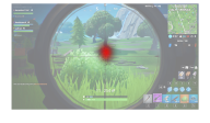
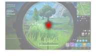
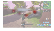
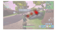
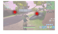
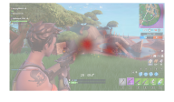
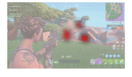
Videogames present an interesting and challenging domain for saliency methods – given their market value, dynamic content, multiple attractors of visual attention, and dependence of human gaze on temporal semantics. We therefore introduce ForGED, a video-saliency dataset with $480$, $13$-second clips of Fortnite game play annotated with gaze data from up to $21$ observers per video. Compared to popular existing datasets such as LEDOV [Jiang et al.(2018)Jiang, Xu, Liu, Qiao, and Wang] and DIEM [Mital et al.(2011)Mital, Smith, Hill, and Henderson], ForGED provides higher dynamism and a video-game context, with the highest number of frames at a consistent $1080$p resolution. We summarize the characteristics of each of the datasets used in our experiments in Tab. 1 and show typical ForGED frames in Fig. 3.

$\tilde{x}_{i}$ with 15 observers	$\tilde{x}_{i}$ with 5 observers	$\tilde{x}_{i}$ with 2 observers	$\tilde{x}_{i}$ with 15 observers	$\tilde{x}_{i}$ with 5 observers	$\tilde{x}_{i}$ with 2 observers
$0.197\pm 0.077$	$0.261\pm 0.136$	$0.478\pm 0.418$	$0.442\pm 0.112$	$0.585\pm 0.277$	$1.018\pm 0.630$
$0.372\pm 0.106$	$0.652\pm 0.324$	$1.079\pm 0.691$	$0.517\pm 0.154$	$0.937\pm 0.453$	$0.947\pm 0.722$

Figure 3: Typical frames from ForGED with gaussian-blurred gaze locations of specified number of observers overlaid in red. For each image, we also show $\operatorname{\mathbb{E}}[\text{KLD}(\tilde{x}_{i}||\tilde{\tilde{x}}_{i})]\pm\text{Std}[\text{KLD}(\tilde{x}_{i}||\tilde{\tilde{x}}_{i})]$. These quantities increase when the saliency map is sparse/multimodal and number of observers is small – a setting that reduces the reliability of a frame for training. ForGED images have been published with the permission from Epic Games.

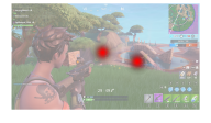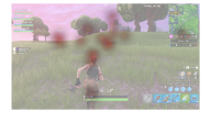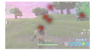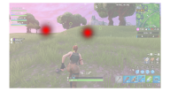Dataset	Videos	Frames	Resolution	Max. Observers	Total Obs.	Content type	mean $\pm$ std.dev.
				used for training	for testing		of optical flow magnitude
DIEM [Mital et al.(2011)Mital, Smith, Hill, and Henderson]	84	240,015	720p@30Hz	31	51-219	everyday videos (shows, advs, etc.)	9.41$\pm$33.85
LEDOV [Jiang et al.(2018)Jiang, Xu, Liu, Qiao, and Wang]	538	179,336	$\geq$720p@24Hz	32	32	human/animal activities	4.09$\pm$8.65
ForGED (ours)	480	374,400	1080p@60hz	5 - 15	15-21	videogame (Fortnite)	27.26$\pm$39.08

Table 1: Characteristics of video-saliency datasets, including the proposed ForGED dataset.

Dynamic content in ForGED.

To compare the dynamic content level of ForGED to those of LEDOV and DIEM, we use RAFT [Teed and Deng(2020)] to compute the mean and standard deviation of the magnitude of the optical flow on a random subset of $100,000$ frames from the three datasets, at a uniform $1080$p resolution and $30$ fps framerate (Tab. 1). This is in ForGED approximately $3\times$ that of DIEM and more than $6\times$ larger than LEDOV, suggesting that objects move faster (on average) in ForGED. It also has the largest standard deviation suggesting a larger variety of motion magnitudes in ForGED.

Gaze data acquisition and viewing behavior in ForGED.

To acquire ForGED, we first recorded 12 hours of Fortnite Battle Royale game-play videos from 8 players of varying expertise using OBS [OBD()]. We then sampled $480$ $15$-second clips to show to a different set of $102$ participants with varying degree of familiarity with Fortnite. Each viewer was tasked with viewing a total of $48$ clips, randomly sampled from the pool of $480$, and interspersed with $3$-second “intervals” showing a central red dot on grey screen [Jiang et al.(2021)Jiang, Xu, Wang, and Sigal] to ensure consistent gaze starting point for each clip (total 15-minute viewing time per viewer). Each participant viewed the video clips on a $1080$p monitor situated approximately 80cm away, while their gaze was recorded with Tobii Tracker 4C at 90Hz. After analyzing the gaze patterns, we discarded the initial $2$ seconds of each clip, when observers were mostly spending time to understand the context, to get a total of $374,400$ video frames annotated with gaze data. Accumulating the gaze of all frames, we observe that ForGED presents a bias towards the frame center and top-right corner. This is because in Fortnite the main character and the crosshair lie at the screen center – making it an important region – and the mini-map on the top right corner attracts regular viewer attention to understand the terrain. Such a bias is uniquely representative of the observer behavior not only in Fortnite, but also in other third person shooting games with similar scene layouts. Further analysis of gaze data in ForGED, such as IOC curves, visual comparison of gaze data biases in ForGED, LEDOV and DIEM, are presented in the Supplementary, Sec. 3.

5 Results

We compare TT (Eq. 2) and NAT (Eq. 7) on three datasets (ForGED, LEDOV [Jiang et al.(2018)Jiang, Xu, Liu, Qiao, and Wang], and DIEM [Mital et al.(2011)Mital, Smith, Hill, and Henderson]) and three DNNs (ViNet [Jain et al.(2021)Jain, Yarlagadda, Jyoti, Karthik, Subramanian, and Gandhi], the state-of-the-art on DHF1K [Wang et al.(2018)Wang, Shen, Guo, Cheng, and Borji]; TASED-Net, a 3D-CNN-based architecture [Min and Corso(2019)]; and SalEMA, an RNN-based architecture [Linardos et al.(2019)Linardos, Mohedano, Nieto, O’Connor, Giro-i Nieto, and McGuinness]). We further evaluate NAT against TT when density-based (e.g, KLD) or fixation-based (e.g, NSS) discrepancy functions are used as $d(\cdot,\cdot)$ in $J^{\text{real}}$ (Eq. 2) and $J_{\text{NAT}}^{\text{real}}$ (Eq. 7). We first evaluated and improved the author-specified hyperparameters for ViNet, TASED-Net, and SalEMA, by performing TT (Eq. 2) on the entire LEDOV training set (see Tab. 2). We use the improved settings for our experiments (see Supplementary Sec. 6). We also verify that training on existing saliency datasets does not generalize to ForGED (Tab. 3c), given its novel content.

method, hyperparameter settings	KLD$\downarrow$	CC$\uparrow$	SIM$\uparrow$	NSS$\uparrow$	AUC-J$\uparrow$
ViNET, Adam, $0.0001$, KLD (default)	$0.806$	$0.697$	$0.569$	$3.781$	$0.881$
ViNET, RMSprop, $0.0001$, KLD (improved)	$\mathbf{0.773}$	$\mathbf{0.710}$	$\mathbf{0.573}$	$\mathbf{3.969}$	$\mathbf{0.889}$
TASED-Net, SGD, learning rate schedule (default)	$1.104$	$0.554$	$0.452$	$2.536$	$0.828$
TASED-Net, RMSprop, $0.001$, KLD (improved)	$\mathbf{0.754}$	$\mathbf{0.724}$	$\mathbf{0.572}$	$\mathbf{4.227}$	$\mathbf{0.921}$
SalEMA, Adam, $1e^{-7}$, BCE (default)	$1.238$	$0.511$	$0.412$	$2.426$	$0.894$
SalEMA, RMSprop, $1e^{-5}$, KLD (improved)	$\mathbf{1.052}$	$\mathbf{0.612}$	$\mathbf{0.463}$	$\mathbf{3.237}$	$\mathbf{0.912}$

Table 2: LEDOV test-set performance when trained (traditionally) with default and improved settings for ViNet [Jain et al.(2021)Jain, Yarlagadda, Jyoti, Karthik, Subramanian, and Gandhi], TASED-Net  [Min and Corso(2019)], and SalEMA [Linardos et al.(2019)Linardos, Mohedano, Nieto, O’Connor, Giro-i Nieto, and McGuinness].

Experimental setup:

We want to compare TT and NAT when training with different amounts of data and varying levels of accuracy/gaze-data completeness. We emulate small-size training datasets from LEDOV, DIEM, and ForGED by controlling the number of fixations, $N$, used to reconstruct $\tilde{x}$ in the training set and the number of training videos, $V$, used. We report the performance evaluation of TT and NAT on test set for each $(V,N)$ value used for the training set. The values for $V$ and $N$ are chosen to gradually increase the training dataset size and accuracy until the maximum $V$ and/or $N$ is reached. To reconstruct $\tilde{x}$, we choose a kernel of size $\sim 1^{\circ}$ viewing angle [Jiang et al.(2021)Jiang, Xu, Wang, and Sigal, Ehinger et al.(2009)Ehinger, Hidalgo-Sotelo, Torralba, and Oliva, Wilming et al.(2011)Wilming, Betz, Kietzmann, and König] and discuss alternative $\tilde{x}$ reconstruction strategies [Kümmerer et al.(2014)Kümmerer, Theis, and Bethge, Kümmerer et al.(2017)Kümmerer, Wallis, Gatys, and Bethge, Kümmerer et al.(2018)Kümmerer, Wallis, and Bethge] in Sec. 6 (and Sec. 7 in the Supplementary).

ForGED data are randomly split into 379 videos for training, 26 for validation, and 75 for testing. For LEDOV, we adopt the train / val / test split specified by the authors. DIEM contains gaze data from many observers on a few videos: we use $60$ videos with fewest observers for training and evaluate on the remaining videos with $51-219$ observers. Evaluation is performed on test-set maps reconstructed from the set of all the available observers, that is sufficiently large to lead to converged IOC curves even for multimodal maps (see supplementary video for ForGED test set multimodality); consequently, we also assume a negligible noise level in evaluation. We omit experimenting with DHF1K in favor of LEDOV which is similar in scope to DHF1K [Tangemann et al.(2020)Tangemann, Kümmerer, Wallis, and Bethge], but contains a larger number of observers (converged IOC curves), while DHF1K lacks accurate per-observer gaze data.

Dataset type and size:

We compare NAT and TT on different dataset types, by training ViNet and TASED-Net on ForGED, LEDOV, and DIEM, and changing $V$ and $N$ to assess the performance gain of NAT as a function of the level of accuracy and completeness of the training dataset. Tab. 3a and 3b show the results for ViNet trained on ForGED and LEDOV, whereas Tab. 4a and 5a show the results for TASED-Net. With ViNet, we observe a consistent performance gain of NAT over TT. Although NAT is particularly advantageous when $N$ and $V$ are small, training on the entire LEDOV dataset (last row in Tab. 3a) also shows a significant improvement for NAT since, depending on their content, some frames can still have insufficient fixation data. With TASED-Net trained on ForGED, NAT consistently outperforms TT when the number of training videos is $\leq 100$, i.e, when noise overfitting may occur. Notably, NAT on 30 videos / 15 observers and 100 videos / 5 observers is comparable or superior to TT with 379 videos / 5 observers, which corresponds to $\geq 3\times$ saving factor in terms of the data required for training. Similar conclusions can be drawn for LEDOV (Tab. 5a) and DIEM (see Supplementary). We also test the case of practical importance of an unbalanced LEDOV dataset, with an uneven number of observers in the training videos. Since NAT, by design, accounts for the varying reliability of the gaze data in training frames, it significantly outperforms TT (last two rows of Tab. 5a).

train videos $V$	train obs. $N$	loss	KLD$\downarrow$	CC$\uparrow$	SIM$\uparrow$	NSS$\uparrow$	AUC-J$\uparrow$
$30$	$5$	TT	$2.636$	$0.266$	$0.250$	$1.344$	$0.528$
		NAT	$\mathbf{2.054}$	$\mathbf{0.406}$	$\mathbf{0.353}$	$\mathbf{1.979}$	$\mathbf{0.624}$
	$15$	TT	$1.475$	$0.467$	$0.414$	$2.320$	$0.779$
		NAT	$\mathbf{1.320}$	$\mathbf{0.502}$	$\mathbf{0.427}$	$\mathbf{2.467}$	$\mathbf{0.813}$
	$25$	TT	$1.717$	$0.446$	$0.395$	$2.286$	$0.708$
		NAT	$\mathbf{1.441}$	$\mathbf{0.482}$	$\mathbf{0.419}$	$\mathbf{2.450}$	$\mathbf{0.786}$
	$30-32$ (all)	TT	$1.828$	$0.448$	$0.392$	$2.281$	$0.663$
		NAT	$\mathbf{1.446}$	$\mathbf{0.491}$	$\mathbf{0.424}$	$\mathbf{2.462}$	$\mathbf{0.770}$
$100$	$30-32$ (all)	TT	$1.303$	$0.539$	$0.453$	$2.676$	$\mathbf{0.798}$
		NAT	$\mathbf{1.275}$	$\mathbf{0.562}$	$\mathbf{0.471}$	$\mathbf{2.848}$	$0.784$
$200$	$30-32$ (all)	TT	$1.066$	$\mathbf{0.611}$	$\mathbf{0.511}$	$\mathbf{3.104}$	$0.840$
		NAT	$\mathbf{1.020}$	$0.598$	$0.503$	$3.025$	$\mathbf{0.869}$
$300$	$30-32$ (all)	TT	$0.959$	$0.655$	$0.535$	$3.456$	$0.847$
		NAT	$\mathbf{0.897}$	$\mathbf{0.669}$	$\mathbf{0.546}$	$\mathbf{3.517}$	$\mathbf{0.863}$
$461$ (all)	$30-32$ (all)	TT	$0.773$	$0.710$	$0.573$	$\mathbf{3.969}$	$0.889$
		NAT	$\mathbf{0.718}$	$\mathbf{0.720}$	$\mathbf{0.577}$	$3.893$	$\mathbf{0.904}$

(a) ViNET on LEDOV, $d=$ KLD

train videos $V$	train obs. $N$	loss	KLD$\downarrow$	CC$\uparrow$	SIM$\uparrow$	NSS$\uparrow$	AUC-J$\uparrow$
$30$	$5$	TT	$1.538$	$0.541$	$0.426$	$3.261$	$0.713$
		NAT	$\mathbf{1.264}$	$\mathbf{0.593}$	$\mathbf{0.460}$	$\mathbf{3.412}$	$\mathbf{0.773}$
	$10$	TT	$1.779$	$0.514$	$0.399$	$3.130$	$0.633$
		NAT	$\mathbf{1.220}$	$\mathbf{0.620}$	$\mathbf{0.488}$	$\mathbf{3.670}$	$\mathbf{0.764}$
	$15$	TT	$\mathbf{1.218}$	$0.602$	$\mathbf{0.473}$	$\mathbf{3.542}$	$\mathbf{0.794}$
		NAT	$1.257$	$\mathbf{0.605}$	$0.469$	$3.527$	$0.773$
$100$	$5$	TT	$1.263$	$0.600$	$0.473$	$3.609$	$0.775$
		NAT	$\mathbf{1.149}$	$\mathbf{0.623}$	$\mathbf{0.485}$	$\mathbf{3.620}$	$\mathbf{0.798}$
$200$	$5$	TT	$1.134$	$0.629$	$\mathbf{0.494}$	$\mathbf{3.750}$	$0.804$
		NAT	$\mathbf{0.982}$	$\mathbf{0.641}$	$0.489$	$3.704$	$\mathbf{0.882}$
$379$	$5$	TT	$\mathbf{0.994}$	$\mathbf{0.645}$	$\mathbf{0.495}$	$\mathbf{3.697}$	$0.860$
		NAT	$1.026$	$0.625$	$0.438$	$3.505$	$\mathbf{0.918}$

(b) ViNET on ForGED, $d=$ KLD

training dataset	KLD$\downarrow$	CC$\uparrow$	SIM$\uparrow$	NSS$\uparrow$	AUC-J$\uparrow$
DHF1K	$2.038$	$0.262$	$0.228$	$1.336$	$0.805$
LEDOV	$1.573$	$0.436$	$0.345$	$2.583$	$0.818$

(c) pretrained ViNET tested on ForGED

Table 3: NAT vs. TT on (a) LEDOV and (b) ForGED with ViNet architecture trained on different training dataset sizes, using $d=$KLD as discrepancy. Best metrics between NAT and TT are in bold. The last two rows in (a) show the training on the entire LEDOV dataset. (c) Training on existing large-scale video-saliency datasets shows poor generalization to ForGED since the videogame presents a very unique visual domain.

train videos $V$	train obs. $N$	loss	KLD$\downarrow$	CC$\uparrow$	SIM$\uparrow$	NSS$\uparrow$	AUC-J$\uparrow$
$30$	$2$	TT	$1.385$	$0.546$	$0.370$	$2.992$	$0.877$
		NAT	$\mathbf{1.298}$	$\mathbf{0.558}$	$\mathbf{0.385}$	$\mathbf{3.161}$	$\mathbf{0.903}$
	$5$	TT	$1.419$	$0.536$	$0.370$	$3.042$	$0.877$
		NAT	$\mathbf{1.172}$	$\mathbf{0.590}$	$\mathbf{0.428}$	$\mathbf{3.372}$	$\mathbf{0.908}$
	$15$	TT	$1.080$	$0.615$	$\mathbf{0.481}$	$3.598$	$0.897$
		NAT	$\mathbf{0.995}$	$\mathbf{0.634}$	$0.478$	$\mathbf{3.750}$	$\mathbf{0.924}$
$100$	$2$	TT	$1.323$	$0.565$	$0.365$	$3.034$	$0.890$
		NAT	$\mathbf{1.056}$	$\mathbf{0.610}$	$\mathbf{0.447}$	$\mathbf{3.386}$	$\mathbf{0.922}$
	$5$	TT	$1.065$	$0.623$	$0.473$	$3.627$	$0.917$
		NAT	$\mathbf{0.969}$	$\mathbf{0.643}$	$\mathbf{0.494}$	$\mathbf{3.749}$	$\mathbf{0.923}$
$379$	$2$	TT	$0.986$	$0.628$	$\mathbf{0.475}$	$3.434$	$0.925$
		NAT	$\mathbf{0.974}$	$\mathbf{0.632}$	$0.470$	$\mathbf{3.497}$	$\mathbf{0.932}$
	$5$	TT	$0.963$	$0.631$	$0.461$	$3.376$	$\mathbf{0.936}$
		NAT	$\mathbf{0.888}$	$\mathbf{0.664}$	$\mathbf{0.508}$	$\mathbf{3.813}$	$0.934$

(a) TASED-Net on ForGED, $d=$ KLD

train videos $V$	train obs. $N$	loss	KLD$\downarrow$	CC$\uparrow$	SIM$\uparrow$	NSS$\uparrow$	AUC-J$\uparrow$
$30$	$5$	TT	$1.155$	$0.612$	$0.440$	$3.600$	$0.904$
		NAT	$\mathbf{1.061}$	$\mathbf{0.618}$	$\mathbf{0.466}$	$\mathbf{3.656}$	$\mathbf{0.912}$
	$15$	TT	$1.095$	$0.612$	$0.448$	$3.574$	$0.919$
		NAT	$\mathbf{0.993}$	$\mathbf{0.639}$	$\mathbf{0.475}$	$\mathbf{3.802}$	$\mathbf{0.928}$
$100$	$2$	TT	$1.138$	$\mathbf{0.601}$	$0.429$	$\mathbf{3.406}$	$0.911$
		NAT	$\mathbf{1.099}$	$0.600$	$\mathbf{0.434}$	$3.356$	$\mathbf{0.920}$
	$5$	TT	$1.097$	$0.623$	$0.425$	$3.533$	$0.921$
		NAT	$\mathbf{1.016}$	$\mathbf{0.631}$	$\mathbf{0.468}$	$\mathbf{3.644}$	$\mathbf{0.924}$
$379$	$2$	TT	$1.069$	$0.618$	$0.436$	$3.456$	$0.920$
		NAT	$\mathbf{1.011}$	$\mathbf{0.626}$	$\mathbf{0.450}$	$\mathbf{3.459}$	$\mathbf{0.931}$
	$5$	TT	$0.958$	$0.655$	$0.467$	$3.652$	$\mathbf{0.934}$
		NAT	$\mathbf{0.905}$	$\mathbf{0.669}$	$\mathbf{0.496}$	$\mathbf{3.946}$	$0.933$

(b) TASED-Net on ForGED, $d=$ KLD - 0.1CC - 0.1NSS

Table 4: NAT vs. TT on ForGED with TASED-Net architecture and different values of $N$,$V$, trained to minimize the discrepancy $d=$ KLD in (a), and $d=$ KLD - 0.1CC - 0.1NSS in (b).

train videos $V$	train obs. $N$	loss	KLD$\downarrow$	CC$\uparrow$	SIM$\uparrow$	NSS$\uparrow$	AUC-J$\uparrow$
$30$	$2$	TT	$2.155$	$0.195$	$0.198$	$1.007$	$0.793$
		NAT	$\mathbf{1.431}$	$\mathbf{0.428}$	$\mathbf{0.378}$	$\mathbf{2.082}$	$\mathbf{0.884}$
	$5$	TT	$1.744$	$0.371$	$0.265$	$1.763$	$0.861$
		NAT	$\mathbf{1.189}$	$\mathbf{0.495}$	$\mathbf{0.409}$	$\mathbf{2.378}$	$\mathbf{0.902}$
	$30$	TT	$1.360$	$0.457$	$0.383$	$2.225$	$0.886$
		NAT	$\mathbf{1.120}$	$\mathbf{0.532}$	$\mathbf{0.433}$	$\mathbf{2.638}$	$\mathbf{0.909}$
$100$	$2$	TT	$1.882$	$0.315$	$0.275$	$1.621$	$0.787$
		NAT	$\mathbf{1.449}$	$\mathbf{0.457}$	$\mathbf{0.367}$	$\mathbf{2.281}$	$\mathbf{0.869}$
	$5$	TT	$1.351$	$0.460$	$0.382$	$2.331$	$0.890$
		NAT	$\mathbf{1.098}$	$\mathbf{0.554}$	$\mathbf{0.443}$	$\mathbf{2.753}$	$\mathbf{0.902}$
	$30$	TT	$1.170$	$0.524$	$0.424$	$2.687$	$0.904$
		NAT	$\mathbf{0.872}$	$\mathbf{0.648}$	$\mathbf{0.493}$	$\mathbf{3.604}$	$\mathbf{0.932}$
$461$	$2$	TT	$1.231$	$0.532$	$0.459$	$2.784$	$0.880$
		NAT	$\mathbf{0.975}$	$\mathbf{0.595}$	$\mathbf{0.499}$	$\mathbf{2.931}$	$\mathbf{0.921}$
	$5$	TT	$\mathbf{0.805}$	$\mathbf{0.684}$	$\mathbf{0.552}$	$\mathbf{3.788}$	$0.921$
		NAT	$0.828$	$0.667$	$0.531$	$3.530$	$\mathbf{0.929}$
	$30-32$ (all)	TT	$0.754$	$0.724$	$0.572$	$\mathbf{4.227}$	$0.921$
		NAT	$\mathbf{0.686}$	$\mathbf{0.727}$	$\mathbf{0.575}$	$4.128$	$\mathbf{0.937}$
	$2,5,15,30$	TT	$0.836$	$0.666$	$\mathbf{0.551}$	$3.615$	$0.916$
		NAT	$\mathbf{0.768}$	$\mathbf{0.692}$	$0.545$	$\mathbf{3.855}$	$\mathbf{0.933}$

(a) TASED-Net on LEDOV, $d=$ KLD

train videos $V$	train obs. $N$	loss	KLD$\downarrow$	CC$\uparrow$	SIM$\uparrow$	NSS$\uparrow$	AUC-J$\uparrow$
$30$	$2$	TT	$1.922$	$0.249$	$0.232$	$1.039$	$0.803$
		NAT	$\mathbf{1.768}$	$\mathbf{0.286}$	$\mathbf{0.285}$	$\mathbf{1.263}$	$\mathbf{0.843}$
	$5$	TT	$2.168$	$0.280$	$0.276$	$1.348$	$0.844$
		NAT	$\mathbf{1.710}$	$\mathbf{0.327}$	$\mathbf{0.298}$	$\mathbf{1.476}$	$\mathbf{0.848}$
	$30$	TT	$1.888$	$0.256$	$0.225$	$1.082$	$0.821$
		NAT	$\mathbf{1.510}$	$\mathbf{0.404}$	$\mathbf{0.321}$	$\mathbf{1.969}$	$\mathbf{0.874}$
$100$	$2$	TT	$1.621$	$0.355$	$0.307$	$1.634$	$0.854$
		NAT	$\mathbf{1.538}$	$\mathbf{0.385}$	$\mathbf{0.311}$	$\mathbf{1.733}$	$\mathbf{0.867}$
	$5$	TT	$1.381$	$0.455$	$0.363$	$2.179$	$0.882$
		NAT	$\mathbf{1.340}$	$\mathbf{0.470}$	$\mathbf{0.392}$	$\mathbf{2.368}$	$\mathbf{0.893}$
	$30$	TT	$1.359$	$0.532$	$0.408$	$2.909$	$0.883$
		NAT	$\mathbf{1.284}$	$\mathbf{0.559}$	$\mathbf{0.408}$	$\mathbf{3.272}$	$\mathbf{0.884}$
$461$	$2$	TT	$1.277$	$0.487$	$0.382$	$2.247$	$0.895$
		NAT	$\mathbf{1.243}$	$\mathbf{0.490}$	$\mathbf{0.403}$	$\mathbf{2.365}$	$\mathbf{0.899}$
	$5$	TT	$1.139$	$\mathbf{0.568}$	$0.444$	$2.825$	$0.903$
		NAT	$\mathbf{1.136}$	$0.567$	$\mathbf{0.450}$	$\mathbf{3.117}$	$\mathbf{0.908}$
	$30$	TT	$1.052$	$0.612$	$\mathbf{0.462}$	$3.237$	$\mathbf{0.912}$
		NAT	$\mathbf{1.045}$	$\mathbf{0.633}$	$0.457$	$\mathbf{3.425}$	$0.910$

(b) SalEMA on LEDOV, $d=$ KLD

Table 5: NAT vs. TT on LEDOV dataset for different DNN architectures – TASED-Net in (a) and SalEMA in (b) – with $d=\text{KLD}$ and different training data sizes. The last two rows in (a) show the case of an unbalanced dataset with $N$ chosen from ${2,5,15,30}$ in a video.

Discrepancy functions:

NAT can be applied to any choice of discrepancy $d$. To demonstrate this, a mix of density- and fixation-based discrepancies, $d=\text{KLD}-0.1\text{CC}-0.1\text{NSS}$, which has also been a popular choice in literature [Droste et al.(2020)Droste, Jiao, and Noble, Wang et al.(2018)Wang, Shen, Guo, Cheng, and Borji], is used to train TASED-Net on ForGED (Tab. 4b). Comparing Tab. 4a and Tab. 4b, we note that NAT provides a performance gain over TT, independently of the training discrepancy. We show more experiments in the Supplementary (Sec. 5), with a fixation-based metric (NSS), and on different datasets.

DNN architectures:

Tab. 5a-b compares NAT vs. TT when training two different DNNs (TASED-Net [Min and Corso(2019)] and SalEMA [Linardos et al.(2019)Linardos, Mohedano, Nieto, O’Connor, Giro-i Nieto, and McGuinness]) on LEDOV, with KLD. As also observed earlier, NAT outperforms TT and the performance gap shrinks with increasing training data. The Supplementary (Sec. 5) shows results with SalEMA on ForGED.

6 Discussion and conclusions

NAT for images: Image-based saliency datasets (e.g, CAT2000 [Borji and Itti(2015)], SALICON [Jiang et al.(2015)Jiang, Huang, Duan, and Zhao]) have many fixations per image resulting in high-quality of the reconstructed saliency maps, as the accuracy rapidly increases with number of fixations (e.g., $>90\%$ accuracy at $20$ fixations [Judd et al.(2012)Judd, Durand, and Torralba]). It is nonetheless fair to ask if NAT is effective for image-saliency predictors.

no. of fixations	loss	KLD$\downarrow$	CC$\uparrow$	SIM$\uparrow$	NSS$\uparrow$	AUC-J$\uparrow$
$5$	TT	$3.986$	$0.578$	$0.537$	$1.477$	$0.764$
	NAT	$\mathbf{1.672}$	$\mathbf{0.660}$	$\mathbf{0.611}$	$\mathbf{1.549}$	$\mathbf{0.817}$
$15$	TT	$2.877$	$0.655$	$0.589$	$1.669$	$0.795$
	NAT	$\mathbf{1.437}$	$\mathbf{0.714}$	$\mathbf{0.640}$	$\mathbf{1.676}$	$\mathbf{0.831}$

Table 6: Evaluation on EML-Net.

We simulate a high-noise, incomplete, dataset by sampling a subset of fixations for each SALICON image and train a state-of-the-art method, EML-Net [Jia and Bruce(2020)], with TT and NAT. Tab. 6 shows the results on the official SALICON benchmark test set, and confirms the advantage of NAT.

Alternative methods to reconstruct $\tilde{x}$:

Although reconstructing $\tilde{x}$ by blurring a binary map of fixations is prevalent practice [Jiang et al.(2021)Jiang, Xu, Wang, and Sigal, Ehinger et al.(2009)Ehinger, Hidalgo-Sotelo, Torralba, and Oliva, Wilming et al.(2011)Wilming, Betz, Kietzmann, and König], we experiment with another reconstruction strategy for $\tilde{x}$ using Gaussian KDE with a uniform regularization. The optimal KDE bandwidth and regularization weight is estimated by optimizing a gold-standard model [Kümmerer et al.(2015)Kümmerer, Wallis, and Bethge, Tangemann et al.(2020)Tangemann, Kümmerer, Wallis, and Bethge] (see Supplementary, Sec. 7). Experiments with TASED-Net on ForGED ($N=5$, $V=30$) comparing TT with $\tilde{x}$ estimated using a fixed-size blur or KDE-based reconstruction, and NAT, show that while KDE improves TT, NAT still yields the best results (Tab. 7).

$\mathbf{\tilde{x}_{i}}$ for training	loss	KLD$\downarrow$	CC$\uparrow$	SIM$\uparrow$	NSS$\uparrow$	AUC-J$\uparrow$
$1^{\circ}$ blur	TT	1.419	0.536	0.370	3.042	0.877
KDE	TT	1.223	0.573	0.399	3.271	0.897
$1^{\circ}$ blur	NAT	1.172	0.590	0.428	3.372	0.908

Table 7: Methods for estimating $\tilde{x}$.

Limitations and future work:

Although the test saliency maps of LEDOV, DIEM and ForGED are derived from several observers leading to converged IOC on average, per-frame inaccuracies of saliency maps can still add uncertainty about the conclusions one can draw. Adopting alternative strategies such as deriving metric-specific saliency from the probabilistic output of a saliency predictor [Bylinskii et al.(2018)Bylinskii, Judd, Oliva, Torralba, and Durand, Kümmerer et al.(2018)Kümmerer, Wallis, and Bethge], can give a clearer understanding. Nonetheless, in our experiments all the metrics are generally in agreement about the ranking between TT and NAT: a strong evidence in favor of NAT [Riche et al.(2013)Riche, Duvinage, Mancas, Gosselin, and Dutoit]. NAT design principles can also be applied to saliency evaluation (not only training), where variable importance is given to each frame depending on its noise level.

Conclusion:

Video gaze data acquisition is time-consuming and can be inaccurate. To reduce the impact of dataset size in the field of visual saliency prediction, we introduce NAT to account for the level of reliability of a saliency map. We also introduce a new dataset which offers a unique video-game context. We show consistent improvements for NAT over TT across a variety of experiments. The adoption of NAT has important practical implications, since it allows acquiring new datasets (or training on old ones) with less data, both in terms of videos and number of observers, without loss of quality.

Noise-Aware Video Saliency Prediction
(Supplementary Material)

 

1 Derivation of NAT cost function (mentioned in Sec. 3)

We interpret $d(x_{i},\tilde{x}_{i})$ as a random variable with Gaussian distribution, $d(x_{i},\tilde{x}_{i})\sim G(\mu_{i},\sigma_{i}^{2})$, where $\mu_{i}=E[d(x_{i},\tilde{x}_{i})]$ indicates its mean, whereas $\sigma_{i}^{2}=\text{Var}[d(x_{i},\tilde{x}_{i})]$ is its variance. When the predicted saliency map $\hat{x}_{i}$ is optimal, i.e, when $\hat{x}_{i}=x_{i}$, $d(\hat{x}_{i},\tilde{x}_{i})$ has the same statistical distribution of $d(x_{i},\tilde{x}_{i})$. Therefore, for a perfect saliency predictor, we can write $d(\hat{x}_{i},\tilde{x}_{i})\sim G(\mu_{i},\sigma_{i}^{2})$. Note that, for our proposed noise-aware training (NAT), $\mu_{i}$ and $\sigma_{i}$ are assumed to be known, and therefore, $\hat{x}_{i}$ is the only unknown. The likelihood of $d(\hat{x}_{i},\tilde{x}_{i})$ is given by:

$$p[d(\hat{x}_{i},\tilde{x}_{i})]=\frac{1}{\sqrt{2\pi}\sigma_{i}}e^{-\frac{[d(\hat{x}_{i},\tilde{x}_{i})-\mu_{i}]^{2}}{2\sigma_{i}^{2}}}.$$ (1)

Given our interpretation of $d(\hat{x}_{i},\tilde{x}_{i})$, for a dataset containing $N+1$ saliency maps, the negative log likelihood is:

$$J(\hat{x}_{0},\hat{x}_{1},...,\hat{x}_{N})=-\text{ln}\prod\nolimits_{i}\frac{1}{\sqrt{2\pi}\sigma_{i}}e^{-\frac{[d(\hat{x}_{i},\tilde{x}_{i})-\mu_{i}]^{2}}{2\sigma_{i}^{2}}}=$$

$$\sum\nolimits_{i}-\text{ln}\{\frac{1}{\sqrt{2\pi}\sigma_{i}}e^{-\frac{[d(\hat{x}_{i},\tilde{x}_{i})-\mu_{i}]^{2}}{2\sigma_{i}^{2}}}\}=$$

$$\sum\nolimits_{i}\{\text{ln}(\sqrt{2\pi}\sigma_{i})+\frac{[d(\hat{x}_{i},\tilde{x}_{i})-\mu_{i}]^{2}}{2\sigma_{i}^{2}}\}.$$ (2)

We want to train the saliency models to predict all the $\{\hat{x}_{i}\}_{i=0...N}$ that maximize the likelihood. Therefore, the optimization problem becomes:

$$(\hat{x}_{0},\hat{x}_{1},...,\hat{x}_{N})=\underset{(\hat{x}_{0},\hat{x}_{1},...,\hat{x}_{N})}{\mathrm{argmin}}J(\hat{x}_{0},\hat{x}_{1},...,\hat{x}_{N})=$$

$$\underset{(\hat{x}_{0},\hat{x}_{1},...,\hat{x}_{N})}{\mathrm{argmin}}\sum\nolimits_{i}\{\text{ln}(\sqrt{2\pi}\sigma_{i})+\frac{[d(\hat{x}_{i},\tilde{x}_{i})-\mu_{i}]^{2}}{2\sigma_{i}^{2}}\}.$$ (3)

Upon simplification (removing the terms that do not depend on $(\hat{x}_{0},\hat{x}_{1},...,\hat{x}_{N})$, that are the only unknowns), we obtain:

$$(\hat{x}_{0},\hat{x}_{1},...,\hat{x}_{N})=\underset{(\hat{x}_{0},\hat{x}_{1},...,\hat{x}_{N})}{\mathrm{argmin}}\sum\nolimits_{i}\{\frac{[d(\hat{x}_{i},\tilde{x}_{i})-\mu_{i}]^{2}}{\sigma_{i}^{2}}\}.$$ (4)

This leads to the formulation of the NAT cost function:

$$J_{\text{NAT}}^{\text{ideal}}=\sum\nolimits_{i}\{\frac{[d(\hat{x}_{i},\tilde{x}_{i})-\mu_{i}]^{2}}{\sigma_{i}^{2}}\}=\sum\nolimits_{i}\{\frac{[d(\hat{x}_{i},\tilde{x}_{i})-\operatorname{\mathbb{E}}[d(x_{i},\tilde{x}_{i})]]^{2}}{\text{Var}[d(x_{i},\tilde{x}_{i})]}\}.$$ (5)

2 A toy example to motivate NAT (mentioned in Sec. 3)

Figure 1: A toy example to motivate NAT. Plots in (a) and (h) show the unimodal and multimonal $1D$ pdfs $x_{i}$ in dashed black lines – these are analogous to the true underlying $2D$ saliency maps for video frames / images. The measured (or training) saliency maps are reconstructed by first sampling “fixations” (red / blue circles in (a, h)) from $x_{i}$, then blurring (b, e, i, l), summing, and normalizing to obtain the resulting reconstructed saliency maps $\tilde{x}_{i}$ (d, g, j, m). When a limited number of observers is available (e.g, 3, in the red plots in (c,j)), the resulting reconstructed $\tilde{x}_{i}$ may differ in shape from $x_{i}$, e.g, due to random shifts, reconstruction errors, etc. Plots d, g, k, n show the expected value and standard deviation for multiple realizations of $\tilde{x}_{i}$, with respect to $x_{i}$. The deviation of $\tilde{x}_{i}$ from $x_{i}$ results in the statistics $\operatorname{\mathbb{E}}[\text{KLD}(x_{i},\tilde{x}_{i})]$ and $\text{Var}[\text{KLD}(x_{i},\tilde{x}_{i})]$ to be non-zero (as shown in the titles of plots d, g, k, n). Furthermore, as is evident from these plots, these statistics are larger when few observers are available and when $x_{i}$ has a complex shape (e.g, multimodal), which makes $x_{i}$ more susceptible to inaccurate approximation using $\tilde{x}_{i}$. The plots considered here for $x_{i}$ are: a Gaussian centered at $\mu=50$, $\sigma=5$; and a mixture with two components at $\mu=[25,75]$, probabilities $P=[0.3,0.7]$, and $\sigma=5$.

Assume that a method predicts the (unobservable) distribution $x_{i}$ exactly, that is $\hat{x}_{i}=x_{i}$. Because of measurement noise and incomplete sampling in $\tilde{x}_{i}$ (which is the the saliency map estimated from insufficient gaze data, i.e, the one typically used for training), $d(x_{i},\tilde{x}_{i})\neq 0$, even though the prediction is perfect. In this scenario, it would suboptimal to train a saliency predictor to minimize $d(x_{i},\tilde{x}_{i})$.

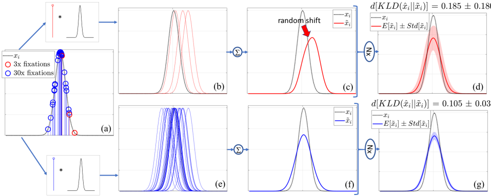
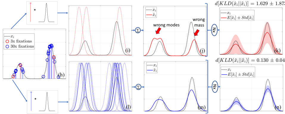
Let us consider a 1D toy example: Figs. 1(a,h) show two 1D ground-truth “saliency maps” (or pdfs) $x_{i}$, one unimodal, and one bimodal. We simulate the “1D gaze-data acquisition” by sampling 3 (red circles) or 30 (blue) spatial locations (or “gaze fixations”) from $x_{i}$. Following the de facto standard to generate saliency maps from single gaze locations, we blur each fixation (Fig. 1(b)), and accumulate the resulting curves (Fig. 1(c)). This results in approximations, $\tilde{x_{i}}$, of the ground-truth saliency maps. The inaccurate positions of the modes in these estimated saliency maps mimics the measurement noise, while the finite number of 1D gaze fixations used to estimate these maps simulates incomplete sampling.

When few fixations are available, $\tilde{x}_{i}$ may be shifted with respect to $x_{i}$ (Fig. 1(c)), and the number of its modes may not match $x_{i}$ (Fig. 1(j)). Furthermore, when $x_{i}$ is multimodal, the mass of each mode in $\tilde{x}_{i}$ may be imprecisely estimated compared to $x_{i}$ (Fig. 1(j)). The standard deviation of $1000$ random realizations of $\tilde{x}_{i}$ ($\text{Std}[\tilde{x}_{i}]$), which measures the uncertainty in $\tilde{x}_{i}$ (and therefore the quality of estimation of $x_{i}$ using $\tilde{x}_{i}$), decreases when a large number of fixations are used to reconstruct $\tilde{x}_{i}$ and remains high for a smaller number of fixations. This is shown as the light-blue / light-red shaded regions in Figs. 1(d, g, k, n), while the solid plot red / blue curve shows $\operatorname{\mathbb{E}}[\tilde{x}_{i}]$. Furthermore, the level of uncertainty is proportional the complexity of the ground-truth saliency map: e.g, given $3$ fixations to reconstruct $\tilde{x_{i}}$, the uncertainty is lower when the underlying ground-truth $x_{i}$ map is unimodal (Fig. 1(d)), and higher when $x_{i}$ is bimodal Fig. 1(k). We note that in Figs. 1(d, g, k, n), $\operatorname{\mathbb{E}}[\tilde{x}_{i}]$ still differs from $x_{i}$ because of the blurring operation used in the reconstruction of $\tilde{x}_{i}$ from sampled 1D locations from $x_{i}$. When the reconstruction process for $\tilde{x}_{i}$ is perfect (a topic of research beyond the scope of this work), such reconstruction errors would be eliminated. For our experiments, we adopt this standard reconstruction process.

The uncertainty in $\tilde{x_{i}}$ due to measurement noise and incomplete sampling results in uncertainty in accurately estimating $d(x_{i},\tilde{x}_{i})$. We now want to estimate the distribution $p[d(x_{i},\tilde{x}_{i})]$, where we model $d(x_{i},\tilde{x}_{i})$ as a Gaussian random variable. We compute $\text{KLD}(x_{i},\tilde{x}_{i})$ for 1,000 random realizations of $\tilde{x}_{i}$ and estimate $\operatorname{\mathbb{E}}[\text{KLD}(x_{i},\tilde{x}_{i})]$, $\text{Std}[\text{KLD}(x_{i},\tilde{x}_{i})]$. These are reported in the titles of Figs. 1(d, g, k, n). We use KLD as discrepancy function because of its wide adoption for saliency estimation, but the results presented here hold for other metrics as well. We observe that:

• $\operatorname{\mathbb{E}}[\text{KLD}(x_{i},\tilde{x}_{i})]>0$, i.e, $\text{KLD}(x_{i},\tilde{x}_{i})$ is biased. The source of the bias is twofold. First, $\text{KLD}(x_{i},\tilde{x}_{i})>0$ because $\operatorname{\mathbb{E}}[\tilde{x}_{i}]$ is a smoothed version of $x_{i}$ (bias due to the choice of the method used to reconstruct $\tilde{x}_{i}$), independently from the number of observers. Second, $\tilde{x}_{i}$ is noisy ($\text{Std}[\tilde{x}_{i}]>0$), which, especially for a limited number of observers, contributes with an additional bias to $\text{KLD}(x_{i},\tilde{x}_{i})$.

• $\text{Std}[\text{KLD}(x_{i},\tilde{x}_{i})]>0$, and it tends to be smaller for a larger number of observers.

• For a given number of observers, $\operatorname{\mathbb{E}}[\text{KLD}(x_{i},\tilde{x}_{i})]$ and $\text{Std}[\text{KLD}(x_{i},\tilde{x}_{i})]$ are larger for multimodal maps.

We conclude that, when $\tilde{x}_{i}$ is affected by measurement noise and incomplete sampling, the expected value and variance of the discrepancy $d(x_{i},\tilde{x}_{i})$ are not zero, depend on the number of observers, and are different for each frame. These properties, which also hold for 2D saliency maps recorded from real human observers, form the basis for the development and interpretation of NAT.

3 Gaze data analysis for ForGED (mentioned in Sec. 4)

Figure 2: Inter-observer consistency (IOC) curve computed on test-set frames of ForGED containing at least $19$ observers. Each data point is an average of the IOC value for the given value of $N$, with the average computed over multiple realizations across the frames. The fitted curve is shown with a solid line and indicates the diminishing amount of new information that gaze data from additional observers imparts, when $N$ is sufficiently high.

Observer consistency and ForGED dataset split.

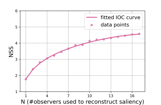
As discussed in Sec. 1 of the main paper, IOC curve measures how well a saliency map reconstructed from gaze data of $N$ observers explains the gaze of a new observer as a function of $N$ [Kümmerer et al.(2015)Kümmerer, Wallis, and Bethge, Wilming et al.(2011)Wilming, Betz, Kietzmann, and König, Jiang et al.(2021)Jiang, Xu, Wang, and Sigal]. A converged IOC curve indicates that additional observers do not add significant new information to the reconstructed saliency map [Jiang et al.(2021)Jiang, Xu, Wang, and Sigal, Judd et al.(2012)Judd, Durand, and Torralba]. A typical test of whether a dataset captures sufficient observers is to evaluate the level of convergence of the IOC curves on average across all frames at maximum value for $N$ (sometimes by using curve-fitting and extrapolation [Judd et al.(2012)Judd, Durand, and Torralba]). To obtain the average IOC for ForGED, we sample $1$ out of every $5$ frames from ForGED test videos containing at least $19$ observers – for a total of $1500$ frames. For each frame, we compute the per-frame IOC curve with $20$ random realizations for the subset of observers that constitute the $N$ observers and the subset that constitutes the new observer whose gaze data is to be explained by the $N$-observer saliency map. All realizations of the IOC curves across all sampled frames are averaged to obtain the IOC curve shown in Fig. 2. As can be seen from Fig. 2, the gradient magnitude of the IOC curve is small at $N=17$ ($0.04$). This further diminishes upon extrapolation to $N=21$ observers to $0.02$. Our test set therefore contains gaze data from up to $21$ observers per video (median $17$). As noted in the main paper (Limitations and Future Work in Sec. 6) - while on average the IOC curves across all evaluated datasets (LEDOV, DIEM, ForGED) show very small gradient at sufficiently high number of observers, the level of convergence for each frame may be different (content-dependent) and motivates the need for NAT. This also presents an interesting direction of future research to design noise-robust evaluation schemes. Note that, while the ForGED test dataset contains gaze data from a large number of observers (that ensures small gradients in the IOC curves at maximum available $N$), the ForGED training dataset consists of a larger number of videos but with gaze data from only $5-15$ observers (the majority of the videos contain $5$ observers). This setting simulates the scenario where training data with limited number of observers is available (the setting most suitable for NAT) – while the testing is always performed on more accurate saliency maps. The training-validation-test split for ForGED videos is $379$ videos for training, $26$ for validation, and $75$ for testing. As already discussed in the main paper (and also shown in Sec. 5), for the different experiments enlisted in tables, the training dataset size is varied in terms of number of available training videos, $V$, and number of observers, $N$, used to reconstruct the saliency maps $\tilde{x_{i}}$ per video – to demonstrate the performance gain of NAT for varying amount of training data.

Figure 3: Accumulated fixation density across gaze data from all observers across all frames in (a) ForGED (b) DIEM and (c) LEDOV.

Observer gaze behavior in ForGED.

Given that the main character is placed at the center of the screen in Fortnite game, we observe an affinity towards center in the gaze behavior. Events such as combat, focused motion towards a location such as the horizon, attempts to pick up resources such as ammunitions lead to observer gaze behavior that follows the narrative of the game-play (e.g, viewers observe the opponent when the main character is in combat, viewers look towards the horizon when the main character is moving towards it). On the other hand, when a scene becomes relatively uneventful, such as when the main central character has been running towards the horizon for a few seconds, the observers’ gaze tends to become more exploratory – scanning the surroundings, or simply browsing the evolving scenery. Examples of all such scenes can be found in the supplementary video, Fig. 3 of the main paper, and Fig. 4 in this Supplementary document. Lastly, we accumulate all of the gaze locations captured on ForGED into a fixation density map (Fig. 3a) to assess the common viewing tendencies of observers. We also compare these for LEDOV and DIEM. As discussed in Sec. 4 of the main paper, due to the main character near the center of the frame, the aiming reticle at the center of the frame, and a guiding mini-map on the top right, observers look at these regions frequently. As compared to LEDOV and DIEM, such a behavior is uniquely representative of the observer behavior in third person shooting games such as Fortnite. In case of LEDOV and DIEM, we also observe a bias towards the center – but it tends to be more widespread as shown in Fig. 3.

4 Analysis of approximation in Eq. 6 (mentioned in Sec. 3)

To analyze the accuracy of Eq. 6 in the main paper, we select a subset of the video frames from the DIEM dataset that contains gaze data from more than $200$ observers. Given the very large number of gaze fixations for these frames, we anticipate that the estimated human-saliency map $\tilde{x_{i}}$ is very close to ground-truth saliency $x_{i}$ [Judd et al.(2012)Judd, Durand, and Torralba] for every such frame $i$ (as also confirmed by converged IOC curves for these frames). We therefore analyze the accuracy of Eq. 6 under the assumption that the $>200$-observer gaze maps of these frames represent $x_{i}$. From these $200$-observer gaze maps ($x_{i}$), we sample a certain number (denoted as $M$) of gaze fixation locations followed by blurring to compute $\tilde{x_{i}}$. Therefore, $\tilde{x}_{i}\ =SR(x_{i};M)$. Then, we compute $\tilde{\tilde{x}}$ by sampling $M$ spatial locations as per the pdf $\tilde{x}$ followed by blurring. That is, $\tilde{\tilde{x_{i}}}\ =SR(\tilde{x_{i}};M)$.

Using multiple realizations of $\tilde{x}$ and $\tilde{\tilde{x}}$, we estimate $\mathbb{E}[d(x,\tilde{x})]$, $\mathbb{E}[d(\tilde{x},\tilde{\tilde{x}})]$, $\text{Var}[d(x,\tilde{x})]$, $\text{Var}[d(\tilde{x},\tilde{\tilde{x}})]$. We find that the mean absolute percentage error (MAPE) in the approximation of $\mathbb{E}[d(x,\tilde{x})]$ (Eq. 6 in main paper) goes from $21\%$ for $N=5$, to $13\%$ for $N=15$, and down to $10\%$ for $N=30$. Similarly, MAPE in the approximation of $\text{Var}[d(x,\tilde{x})]$ (Eq. 6 in main paper) goes from $13\%$ for $N=5$, to $6\%$ for $N=15$, and down to $5\%$ for $N=30$. Note that a large under/over-estimation of $\mathbb{E}[d(x,\tilde{x})]$ and $\text{Var}[d(x,\tilde{x})]$ in Eq. 6 (main paper) may lead to overfitting to noisy data or sub-optimal convergence respectively using Eq. 7 (main paper) for training. This would result in poor performance of NAT compared to traditional training – which, as shown by the results, is not the case.

5 Additional Results (mentioned in Sec. 5)

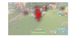
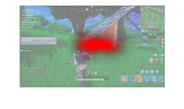
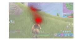
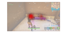
We now report the additional experiments performed to compare NAT (Eq. 6 in main paper) to traditional training (abbreviated as TT in this section; Eq. 2 in main paper). Furthermore, we show typical gaze maps obtained through TT and NAT compared to the ground truth for TASED on the ForGED dataset in Fig. 4.

5.1 Dataset type and size

In this section, we continue reporting the results from Sec. 5 of the main paper, where we compared NAT vs. TT for different dataset types and sizes. Table 1 compares the performance of TT to NAT on an additional dataset, the DIEM dataset [Mital et al.(2011)Mital, Smith, Hill, and Henderson], for the TASED architecture [Min and Corso(2019)], and using KLD as discrepancy for training. As done throughout Sec. 5 of the main paper, the evaluation on test set of DIEM is performed on videos with gaze data from all of the available observers (in contrast to training, for which a subset of observers are used, see Table 1 in main paper). In case of DIEM dataset, given that only $84$ videos are available, we use $30$ or $60$ videos for training and report the results on the remaining $24$ videos, which are also used as validation set. The number of observers for these videos ranges from $51$ to $219$, which makes DIEM a very low-noise evaluation set [Judd et al.(2012)Judd, Durand, and Torralba]. Results on DIEM are consistent with those reported in the main paper, with NAT providing better metrics in evaluation when compared to TT when less training data (e.g., $30$ videos) is available.

train videos $V$	train obs. $N$	loss	KLD$\downarrow$	CC$\uparrow$	SIM$\uparrow$	NSS$\uparrow$	AUC-J$\uparrow$
$30$	$5$	TT	$0.641$	$0.698$	$0.591$	$\mathbf{3.517}$	$0.922$
		NAT	$\mathbf{0.599}$	$\mathbf{0.708}$	$\mathbf{0.592}$	$3.513$	$\mathbf{0.934}$
	$15$	TT	$0.597$	$0.710$	$0.602$	$3.582$	$0.930$
		NAT	$\mathbf{0.583}$	$\mathbf{0.718}$	$\mathbf{0.607}$	$\mathbf{3.627}$	$\mathbf{0.932}$
	$31$	TT	$0.576$	$0.724$	$0.614$	$3.663$	$0.925$
		NAT	$\mathbf{0.559}$	$\mathbf{0.731}$	$\mathbf{0.618}$	$\mathbf{3.694}$	$\mathbf{0.928}$
$60$	$5$	TT	$0.528$	$0.735$	$\mathbf{0.619}$	$\mathbf{3.709}$	$0.933$
		NAT	$\mathbf{0.518}$	$\mathbf{0.737}$	$0.616$	$3.639$	$\mathbf{0.940}$
	$15$	TT	$\mathbf{0.485}$	$\mathbf{0.757}$	$\mathbf{0.639}$	$\mathbf{3.795}$	$0.933$
		NAT	$0.493$	$0.754$	$0.635$	$3.792$	$\mathbf{0.936}$
	$31$	TT	$0.476$	$0.759$	$0.641$	$3.821$	$\mathbf{0.938}$
		NAT	$\mathbf{0.467}$	$\mathbf{0.766}$	$\mathbf{0.654}$	$\mathbf{3.864}$	$0.935$

Table 1: Saliency metrics on DIEM, for TASED Net, training with KLD as discrepancy, and various number of training videos and observers. The best metrics between TT (Eq. 2 in main paper) and NAT are in bold.

measured $\tilde{x}_{i}$
	KLD=1.48, CC=0.52	KLD=0.88, CC=0.78	KLD=1.40, CC=0.47	KLD=1.22, CC=0.52
TT
	KLD=0.82, CC=0.77	KLD=0.59, CC=0.69	KLD=0.54, CC=0.75	KLD=1.28, CC=0.51
NAT

Figure 4: Typical gaze maps obtained through TT (second row – Eq. 2 in main paper) and NAT (third row) compared to the ground truth (first row) for TASED on the ForGED dataset, training with KLD loss, 30 training videos and 5 observers per frame (see Table 4a in main paper). Each panel reports in the title the corresponding KLD and CC values. The last column shows a failure case where the metrics KLD and CC indicate that NAT is worse than TT, although a visual inspection might indicate otherwise. Furthermore, the saliency maps predicted with TT indicate more centralized unimodal predictions – while NAT accurately predicts decentralized, multi-modal saliency maps even when trained with less data. The visualization of saliency map overlays follows the scheme in Fig. 3 of main paper. ForGED images have been published with permission of Epic Games.

5.2 Discrepancy functions

Table 2 shows NAT vs. TT using $d=-\text{NSS}$ on ForGED dataset. In Table 2, we notice that NAT overcomes TT in terms of NSS only for 2 or 5 observers, and 30 training videos. Recall that, by design, NSS optimizes the predicted saliency map only at the measured fixation locations. Consequently, when few fixations per frame are available for training, a high NSS score may not generalize well to other evaluation metrics that evaluate different aspects of the quality of a predicted saliency map. This can be alleviated by additional regularization (such as using additional metrics as we do with $d=\text{KLD}-0.1\text{CC}-0.1\text{NSS}$ in Table 4b of the main paper and observe that high NSS scores generalize to good performance in terms of other metrics). In other words, for few-observer training, optimizing for NSS alone may not constrain the predicted saliency map sufficiently — which shows up as poor generalization to other metrics. This is what we observe in Table 2, where the regularizing effect of NAT leads to worse NSS values compared to TT; but, all of the other evaluation metrics indicate NAT to be better.

train videos $V$	train obs. $N$	loss	KLD$\downarrow$	CC$\uparrow$	SIM$\uparrow$	NSS$\uparrow$	AUC-J$\uparrow$
$30$	$2$	TT	$2.005$	$0.362$	$0.302$	$2.677$	$0.788$
		NAT	$\mathbf{1.408}$	$\mathbf{0.528}$	$\mathbf{0.371}$	$\mathbf{3.163}$	$\mathbf{0.887}$
	$5$	TT	$1.642$	$0.489$	$0.28$	$3.212$	$0.898$
		NAT	$\mathbf{1.254}$	$\mathbf{0.566}$	$\mathbf{0.417}$	$\mathbf{3.39}$	$\mathbf{0.906}$
	$15$	TT	$1.518$	$0.506$	$0.403$	$\mathbf{3.672}$	$0.826$
		NAT	$\mathbf{1.155}$	$\mathbf{0.608}$	$\mathbf{0.435}$	$3.552$	$\mathbf{0.91}$
$100$	$2$	TT	$1.328$	$0.563$	$0.383$	$\mathbf{3.783}$	$0.899$
		NAT	$\mathbf{1.206}$	$\mathbf{0.584}$	$\mathbf{0.426}$	$3.44$	$\mathbf{0.906}$
	$5$	TT	$1.312$	$0.578$	$0.452$	$\mathbf{3.983}$	$0.835$
		NAT	$\mathbf{1.165}$	$\mathbf{0.61}$	$\mathbf{0.475}$	$3.747$	$\mathbf{0.879}$
$379$	$2$	TT	$1.163$	$0.614$	$0.475$	$\mathbf{4.161}$	$0.857$
		NAT	$\mathbf{1.028}$	$\mathbf{0.642}$	$\mathbf{0.495}$	$3.858$	$\mathbf{0.901}$
	$5$	TT	$1.093$	$0.633$	$0.491$	$\mathbf{4.381}$	$0.875$
		NAT	$\mathbf{1.006}$	$\mathbf{0.658}$	$\mathbf{0.512}$	$3.928$	$\mathbf{0.892}$

Table 2: NAT vs. TT on ForGED for TASED, $d=-\text{NSS}$ (a fixation-based discrepancy), various number of training videos and observers. Best metrics for each pair of experiments in bold.

To further verify that NAT generalizes to different discrepancy functions, we train and test TASED on LEDOV [Jiang et al.(2018)Jiang, Xu, Liu, Qiao, and Wang] with the fixation-based discrepancy function, $d=-\text{NSS}$, and the combination of fixation and density-based discrepancy functions, $d=\text{KLD}-0.1\text{CC}-0.1\text{NSS}$ (which is a popular discrepancy function used in video-saliency research [Droste et al.(2020)Droste, Jiao, and Noble, Wang et al.(2018)Wang, Shen, Guo, Cheng, and Borji]). The test set for LEDOV is used for all reported evaluations on LEDOV dataset, which contains gaze data from $32$ observers per video.

Table 3 shows NAT vs. TT (Eq. 2 in main paper) using $d=-\text{NSS}$. For this specific experiment, with TT we observe that adopting RMSprop as the optimizer (as done for all experiments in the paper) shows very fast convergence to very high NSS values. While this property of fast and optimal convergence of discrepancy function has proven useful for all experiments in the paper (see Sec. 6 for details), for this specific experiment the solution provided by RMSprop optimization shows poor generalization to all other saliency metrics. This behavior is alleviated to some extent by switching RMSProp with Stochastic Gradient Descent (SGD) for TT – but at the cost of poor convergence in terms of NSS. To show this, in Table 3, we report two sets of experiments for TT for each size of training dataset (one with SGD and another with RMSprop). With NAT, however, we observe a consistent optimal convergence due to the regularizing effect of the NAT formulation that prevents overfitting to dataset noise.

We further observe that using additional terms with NSS in the discrepancy function, such as with $d=\text{KLD}-0.1\text{CC}-0.1\text{NSS}$ overcomes some of the issues of training with NSS alone. Table 4, 5 show the comparison of TT vs. NAT for this combined discrepancy function. A high NSS performance in this case is well-correlated with good performance in terms of other metrics. Furthermore we note that the performance of NAT is superior to TT when less gaze data is available, with the gap between the two approaches closing in with more gaze data. Given our analyses of all of the experiments with various discrepancy functions and dataset types, our conclusion is that the performance of models trained with density-based discrepancy functions (e.g., KLD) is better for TT as well as NAT, with NAT showing consistent superior performance compared to TT.

train videos $V$	train obs. $N$	loss	KLD$\downarrow$	CC$\uparrow$	SIM$\uparrow$	NSS$\uparrow$	AUC-J$\uparrow$
$100$	$5$	TT, SGD	$\mathit{2.352}$	$\mathit{0.244}$	$\mathbf{0.267}$	$2.272$	$\mathit{0.761}$
		TT, RMSprop	$4.139$	$0.192$	$0.056$	$\mathbf{9.92}$	$0.178$
		NAT	$\mathbf{1.746}$	$\mathbf{0.428}$	$\mathit{0.230}$	$\mathit{2.358}$	$\mathbf{0.916}$
	$30$	TT, SGD	$\mathit{2.302}$	$\mathit{0.258}$	$\mathbf{0.275}$	$\mathit{2.661}$	$\mathit{0.775}$
		TT, RMSprop	$3.593$	$0.247$	$0.111$	$\mathbf{13.628}$	$0.423$
		NAT	$\mathbf{1.903}$	$\mathbf{0.398}$	$\mathit{0.198}$	$2.370$	$\mathbf{0.919}$
$461$	$5$	TT, SGD	$\mathit{2.777}$	$\mathit{0.317}$	$\mathit{0.232}$	$\mathit{4.464}$	$\mathit{0.612}$
		TT, RMSprop	$4.00$	$0.241$	$0.062$	$\mathbf{14.617}$	$0.206$
		NAT	$\mathbf{1.305}$	$\mathbf{0.575}$	$\mathbf{0.354}$	$3.29$	$\mathbf{0.929}$
	$30$	TT, SGD	$\mathit{2.252}$	$\mathit{0.470}$	$\mathbf{0.355}$	$2.463$	$\mathit{0.593}$
		TT, RMSprop	$3.526$	$0.292$	$0.127$	$\mathbf{14.048}$	$0.381$
		NAT	$\mathbf{1.402}$	$\mathbf{0.571}$	$\mathit{0.310}$	$\mathit{2.933}$	$\mathbf{0.927}$

Table 3: Comparison of TT (Eq. 2 in main paper) vs. NAT on LEDOV testing set, for TASED Net, trained with $-0.1\text{NSS}$ as discrepancy, and various number of training videos and observers. The best metric between each set of 3 experiments for a given dataset size (videos and observers) is in bold and the second-best is italicized. Given the strong overfitting behavior of NSS with TT using RMSprop for this particular set of experiments, we report TT optimized with SGD as well.

train videos $V$	train obs. $N$	loss	KLD$\downarrow$	CC$\uparrow$	SIM$\uparrow$	NSS$\uparrow$	AUC-J$\uparrow$
$30$	$30$	TT	$1.652$	$0.446$	$0.261$	$2.269$	$0.871$
		NAT	$\mathbf{1.243}$	$\mathbf{0.494}$	$\mathbf{0.394}$	$\mathbf{2.491}$	$\mathbf{0.900}$
$100$	$5$	TT	$1.368$	$0.496$	$0.395$	$2.430$	$0.863$
		NAT	$\mathbf{1.149}$	$\mathbf{0.540}$	$\mathbf{0.423}$	$\mathbf{2.782}$	$\mathbf{0.905}$
	$30$	TT	$1.261$	$0.534$	$0.368$	$2.658$	$0.903$
		NAT	$\mathbf{1.034}$	$\mathbf{0.574}$	$\mathbf{0.432}$	$\mathbf{3.250}$	$\mathbf{0.928}$
$461$	$5$	TT	$1.159$	$0.577$	$0.485$	$\mathbf{3.912}$	$0.864$
		NAT	$\mathbf{0.852}$	$\mathbf{0.626}$	$\mathbf{0.513}$	$3.451$	$\mathbf{0.931}$
	$30$	TT	$0.913$	$0.626$	$0.513$	$\mathbf{5.743}$	$0.910$
		NAT	$\mathbf{0.755}$	$\mathbf{0.688}$	$\mathbf{0.554}$	$3.559$	$\mathbf{0.930}$

Table 4: Saliency quality metrics on LEDOV testing set, for TASED Net, training with KLD-0.1CC-0.1NSS as discrepancy, and various number of training videos and observers. The best metrics between TT (Eq. 2 in main paper) and NAT are in bold.

train videos $V$	train obs. $N$	loss	KLD$\downarrow$	CC$\uparrow$	SIM$\uparrow$	NSS$\uparrow$	AUC-J$\uparrow$
$30$	$15$	TT	$0.687$	$0.696$	$0.590$	$3.618$	$0.900$
		NAT	$\mathbf{0.588}$	$\mathbf{0.718}$	$\mathbf{0.601}$	$\mathbf{3.629}$	$\mathbf{0.932}$
	$31$	TT	$\mathbf{0.555}$	$0.727$	$0.609$	$3.605$	$\mathbf{0.935}$
		NAT	$0.560$	$\mathbf{0.730}$	$\mathbf{0.612}$	$\mathbf{3.666}$	$0.933$
$60$	$5$	TT	$0.555$	$0.728$	$\mathbf{0.615}$	$3.660$	$0.930$
		NAT	$\mathbf{0.535}$	$\mathbf{0.736}$	$0.612$	$\mathbf{3.681}$	$\mathbf{0.937}$
	$15$	TT	$0.514$	$0.743$	$0.631$	$3.804$	$0.931$
		NAT	$\mathbf{0.488}$	$\mathbf{0.755}$	$\mathbf{0.636}$	$\mathbf{3.814}$	$\mathbf{0.939}$
	$31$	TT	$\mathbf{0.502}$	$0.748$	$\mathbf{0.639}$	$\mathbf{3.887}$	$0.931$
		NAT	$0.503$	$\mathbf{0.750}$	$0.632$	$3.774$	$\mathbf{0.938}$

Table 5: Saliency quality metrics on DIEM testing set, for TASED Net, training with KLD-0.1CC-0.1NSS as discrepancy, and various number of training videos and observers. The best metrics between TT (Eq. 2 in main paper) and NAT are in bold.

5.3 DNN architectures

To further verify that NAT works effectively on different DNN architectures, independently from the adopted dataset, we train SalEMA [Linardos et al.(2019)Linardos, Mohedano, Nieto, O’Connor, Giro-i Nieto, and McGuinness] on the ForGED dataset. We use KLD as the discrepancy function, with RMSprop as the optimizer with a learning rate equal to $1e^{-5}$ rather than Adam with learning rate $1e^{-7}$ and binary cross entropy as discrepancy function, as suggested by the authors (an analysis of this hyperparameter choice is discussed later). Consistently with the other cases analyzed here, NAT outperforms TT, notably when the number of observers or videos is limited (Table 6).

train videos $V$	train obs. $N$	loss	KLD$\downarrow$	CC$\uparrow$	SIM$\uparrow$	NSS$\uparrow$	AUC-J$\uparrow$
$30$	$5$	TT	$1.229$	$0.546$	$0.412$	$2.911$	$0.912$
		NAT	$\mathbf{1.187}$	$\mathbf{0.559}$	$\mathbf{0.428}$	$\mathbf{3.050}$	$\mathbf{0.915}$
	$15$	TT	$1.214$	$0.544$	$0.420$	$2.972$	$0.916$
		NAT	$\mathbf{1.184}$	$\mathbf{0.563}$	$\mathbf{0.426}$	$\mathbf{3.152}$	$\mathbf{0.916}$
$100$	$5$	TT	$1.077$	$\mathbf{0.600}$	$0.444$	$3.273$	$0.923$
		NAT	$\mathbf{1.071}$	$0.599$	$\mathbf{0.447}$	$\mathbf{3.274}$	$\mathbf{0.926}$
$379$	$2$	TT	$\mathbf{1.054}$	$\mathbf{0.601}$	$\mathbf{0.447}$	$3.248$	$0.926$
		NAT	$1.076$	$0.600$	$0.440$	$\mathbf{3.284}$	$\mathbf{0.930}$
	$5$	TT	$\mathbf{1.014}$	$0.623$	$\mathbf{0.482}$	$\mathbf{3.533}$	$0.929$
		NAT	$1.019$	$\mathbf{0.623}$	$0.471$	$3.526$	$\mathbf{0.930}$

Table 6: Saliency quality metrics on ForGED testing set, for SalEMA, training with KLD as discrepancy, and various number of training videos and observers. The best metrics between TT (Eq. 2 in main paper) and NAT are in bold.

6 Additional training details (mentioned in Sec. 5)

Hyperparameters for TASED training on LEDOV.

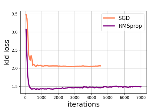
To ensure a fair comparison against traditional training and guarantee that the best performance are achieved for the given architecture and dataset, we first perform some hyperparameter tuning of TASED on LEDOV with traditional training (Eq. 2 in main paper). We found that using RMSprop with a learning rate of $0.001$ for KLD optimization gives better performance than the default settings originally proposed for training on DHF1K (i.e,, SGD with momentum $0.9$ and learning rate $0.1$ for decoder stepping down by a factor of $0.1$ at iteration $750$ and $950$, and $0.001$ for encoder), as shown in Table 7 and in Fig. 5. Thus, we adopt RMSprop with a learning rate of $0.001$ to train TASED for both traditional training and NAT in all the experiments. An exception to this rule is the traditional training with SGD reported in Table 3, where we adopt SGD with a learning rate of $0.0001$ (any higher leads to training instabilities due to data noise) and momentum $0.9$.

Figure 5: Validation-set performance plots (KLD vs. training iterations) for the LEDOV dataset during training of TASED with KLD as loss function and LEDOV dataset using: SGD, initial learning rate $0.1$ for decoder and $0.001$ for encoder, momentum $0.9$ (default used by authors); and RMSprop, learning rate $0.001$. Based on this experiment, we choose RMSprop with a learning rate of $0.001$ for our experiments.

hyperparameter settings	KLD$\downarrow$	CC$\uparrow$	SIM$\uparrow$	NSS$\uparrow$	AUC-J$\uparrow$
TASED-Net, SGD, learning rate schedule (default)	$1.104$	$0.554$	$0.452$	$2.536$	$0.828$
TASED-Net, RMSprop, $0.001$, KLD (improved)	$\mathbf{0.754}$	$\mathbf{0.724}$	$\mathbf{0.572}$	$\mathbf{4.227}$	$\mathbf{0.921}$

Table 7: Performance on LEDOV for TASED trained traditionally using KLD with original settings, and those used in the main paper (RMSprop, learning rate $0.001$) on the full LEDOV training set. We adopted the best hyperparameter setting (best metrics in bold) for all experiments. *Original settings: SGD, initial learning rate $0.1$ for decoder and $0.001$ for encoder, momentum $0.9$.

Hyperparameters for SalEMA training on LEDOV.

We train SalEMA [Linardos et al.(2019)Linardos, Mohedano, Nieto, O’Connor, Giro-i Nieto, and McGuinness] on the full LEDOV dataset with the default choice for loss function and optimizer (Adam optimizer, binary cross entropy, with learning rate $1e^{-7}$), and compare against the adoption of the RMSprop optimizer with KLD as the loss function and $2$ learnings rates: $1e^{-5}$ and $1e^{-7}$ (see Table. 8). We train with LEDOV training set and we choose the best hyperparameter setting based on the LEDOV test-set performance for all of the experiments in the paper.

hyperparameter settings	KLD$\downarrow$	CC$\uparrow$	SIM$\uparrow$	NSS$\uparrow$	AUC-J$\uparrow$
Adam, $1e^{-7}$, BCE (original)	$1.238$	$0.511$	$0.412$	$2.426$	$0.894$
RMSprop, $1e^{-7}$, KLD	$1.206$	$0.532$	$0.418$	$2.602$	$0.900$
RMSprop, $1e^{-5}$, KLD	$\mathbf{1.052}$	$\mathbf{0.612}$	$\mathbf{0.463}$	$\mathbf{3.237}$	$\mathbf{0.912}$

Table 8: Performance comparisons on LEDOV test set for SalEMA trained with the original hyperaprameter settings and the ones used in this paper (RMPprop optimizer with $1e^{-5}$ learning rate) after training on LEDOV training set. Best metrics are in bold.

Details of training EML-Net.

We train EML-Net [Jia and Bruce(2020)] for image-saliency on our noisy version of SALICON train set [Jiang et al.(2015)Jiang, Huang, Duan, and Zhao] (generated by randomly selecting a subset $5$ or $15$ fixations per image, see Sec. 6 in main paper). To do so, we select the ResNet50 backbone [He et al.(2016)He, Zhang, Ren, and Sun]. Consistent with recommendations from authors, we train two versions of the encoder: first, we finetune starting from ImageNet-pretrained weights [Russakovsky et al.(2015)Russakovsky, Deng, Su, Krause, Satheesh, Ma, Huang, Karpathy, Khosla, Bernstein, et al.], and second, we finetune from Places365-pretrained weights [Zhou et al.(2017)Zhou, Lapedriza, Khosla, Oliva, and Torralba]. The two saliency models obtained from the encoder-training stage are input to the decoder-training pipeline to give the final image-saliency predictor for EML-Net approach. We adopt the EML discreapncy (which is a combination of KLD, CC and NSS losses described by authors) for training both traditionally (Eq. 2 in main paper) and using NAT. After searching through learning rates and optimizers, we find the author-specified choices to be most optimal: SGD with momentum with a learning rate of $0.01$ at the beginning and multiplied by $0.1$ after every epoch. We train both encoder and decoder for $10$ epochs. After training, the best model for each experiment in Table 6 of the main paper is selected based on validation-set performance (using all available fixations on images in validation set), and submitted to SALICON benchmark for evaluation on the test set [Jiang et al.(2015)Jiang, Huang, Duan, and Zhao]. Note that even though the training is performed on few-fixation images to simulate a noisy version of the SALICON dataset, the evaluation on test set and validation set contains all of the available fixations.

7 Alternative methods to estimate $\tilde{x}$ (mentioned in Sec. 6)

In Sec. 6 of main paper, we discuss an alternative strategy using Gaussian kernel density estimation (KDE) with uniform regularizer to estimate $\tilde{x}$ for training, instead of the common practice of blurring human gaze fixation locations using a Gaussian blur kernel of size approximately $1^{\circ}$ viewing angle. We provide further details here. We estimate the optimal KDE bandwidth for each video frame, mixed with a uniform regularizer whose coefficient is also a parameter to be estimated. We do a per-frame estimation of optimal KDE bandwidth and mixing coefficient, to account for the general case where each frame can have a different variety of points of interest to attract gaze which cannot be explained with the optimal KDE bandwidth of another frame. The alternative to this is to estimate an optimal KDE bandwidth independent of the video frames, which amounts to the case of obtaining a universal Gaussian-blur kernel of a different size. In this case, the treatment of the underlying gaze data for obtaining the measured saliency maps, $\tilde{\tilde{x_{i}}}$, remains the same, in principle, as our experiments with $\sim 1^{\circ}$ viewing-angle Gaussian-blur kernel (which amounts to $36$ pixels and $1920\times 1080$ resolution for ForGED). To demonstrate this for completeness, in Table 9, we show some of the results for TASED trained with ForGED and KLD as discrepancy. For this experiment, the training gaze maps are estimated using a Gaussian-blur kernel of size $27$ pixels (at resolution $1920\times 1080$), which amounts to $\sim 0.75^{\circ}$ viewing angle. We note in Table 9 that NAT outperforms traditional training, consistent with our experiments with $\sim 1^{\circ}$ viewing-angle Gaussian-blur kernel reported in the main paper.

train videos $V$	train obs. $N$	loss	KLD$\downarrow$	CC$\uparrow$	SIM$\uparrow$	NSS$\uparrow$	AUC-J$\uparrow$
$30$	$2$	TT	$1.586$	$0.471$	$0.329$	$2.832$	$0.878$
		NAT	$\mathbf{1.387}$	$\mathbf{0.546}$	$\mathbf{0.378}$	$\mathbf{3.153}$	$\mathbf{0.879}$
	$5$	TT	$1.358$	$0.563$	$0.345$	$3.184$	$0.903$
		NAT	$\mathbf{1.239}$	$\mathbf{0.565}$	$\mathbf{0.406}$	$\mathbf{3.272}$	$\mathbf{0.905}$
	$15$	TT	$1.056$	$\mathbf{0.622}$	$\mathbf{0.483}$	$3.682$	$0.902$
		NAT	$\mathbf{1.035}$	$0.616$	$0.476$	$\mathbf{3.757}$	$\mathbf{0.917}$
$100$	$5$	TT	$1.085$	$0.634$	$0.464$	$\mathbf{3.770}$	$0.903$
		NAT	$\mathbf{1.018}$	$\mathbf{0.636}$	$\mathbf{0.474}$	$3.633$	$\mathbf{0.926}$
$379$	$5$	TT	$0.959$	$0.651$	$0.480$	$3.652$	$\mathbf{0.931}$
		NAT	$\mathbf{0.888}$	$\mathbf{0.670}$	$\mathbf{0.517}$	$\mathbf{4.091}$	$0.924$

Table 9: Performance comparisons on ForGED test set for TASED trained with KLD as discrepancy. Instead of computing gaze maps for train set with Gaussian blur kernel of size approximately $1^{\circ}$ viewing angle (which amounts of $36$ pixels at $1920\times 1080$ resolution), we use a Gaussian blur kernel of size approximately $0.75^{\circ}$ viewing angle ($27$ pixels). As we can see, the conclusion regarding the superior performance of NAT compared to traditional training applies independent of blur kernel size.

To estimate the optimal bandwidth using KDE, we optimize a gold-standard model for saliency prediction, which predicts the probability of fixation for one observer, given the gaze data from the remaining observers for the video frame (leave-one-out cross-validation) [Kümmerer et al.(2015)Kümmerer, Wallis, and Bethge, Tangemann et al.(2020)Tangemann, Kümmerer, Wallis, and Bethge]. We observe that, when gaze fixation locations are sparsely distributed across a frame, the optimal bandwidth for KDE is high, which would result is high-spread, almost-uniform saliency maps. Independent of the estimation strategy for $\tilde{x}$, we posit that there is an underlying uncertainty / noise in the measured saliency map – which is accounted for during training using NAT, to obtain improved performance over traditional training.

Figure 6: Training-set and validation-set KLD as a function of training iterations for TASED trained on LEDOV (“GT” in the legend indicates “ground-truth”). In contrast to the traditional training (Eq.2 in main paper), NAT does not overfit.

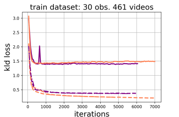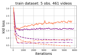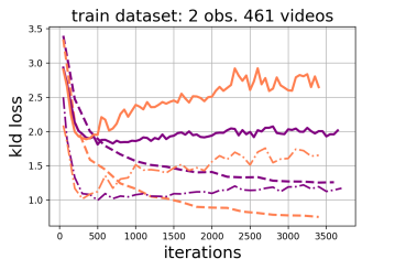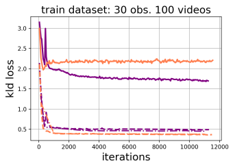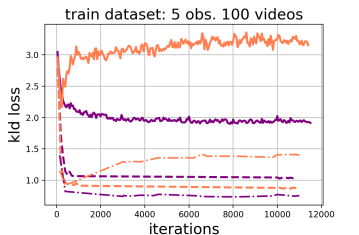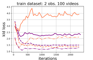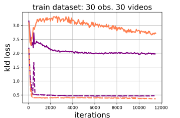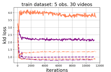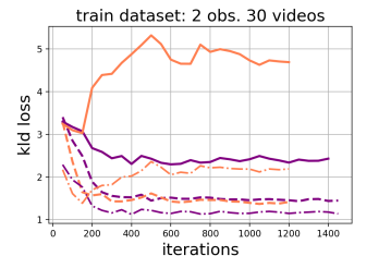8 Overfitting behavior with NAT (mentioned in Sec. 3)

Figure 6 shows the training and validation set performance (in terms of KLD) as a function of the training iteration when training TASED on LEDOV dataset with KLD discrepancy, for different number of observers and videos in the training set. For both the traditional approach (dashed orange line) and NAT (dashed purple line), the training-set curves decrease regularly, as expected in a smooth optimization process. However, the validation-set curves for traditional training (continuous orange line) quickly reach a minimum and then start diverging towards a higher asymptotic value, which is a clear sign of overfitting. On the other hand, the validation curves for NAT (continuous purple line) are always lower (suggesting better performance) and tend to stabilize around asymptotic values without growing anymore — a clear sign, in this case, that overfitting is avoided. Note that for the training-set curves (dashed lines), the human saliency map used for KLD computation is derived using the limited number of observers available during the specific training experiment. As an additional check for the overfitting behavior of traditional training, we plot the performance of training set when compared against human saliency maps obtained from all the observers available in the training videos ($32$). These are indicated with dash-dotted lines. For few-observer experiments, the performance of traditional training on all-observer evaluations gets worse with increasing iterations. On the contrary, the performance on validation set, training set, and all-observer training set do not generally show signs of overfitting for NAT. Only in few cases, NAT plots are unstable at the beginning of the training (see the peaks in the validation curves in the left most panels for $30$ observers trainings), but then the curves stabilize to an asymptotic value. The only exception to this is represented by the upper right panel in the figure ($2$-observer training with $461$ videos), where we believe that the slight increase in the validation-set performance value is due to the approximation introduced in NAT to make it computable in practice. We observed a similar behavior when training on other datasets.

References

- [OBD()] Open broadcaster software. https://obsproject.com/.
- [Alletto et al.(2016)Alletto, Palazzi, Solera, Calderara, and Cucchiara] Stefano Alletto, Andrea Palazzi, Francesco Solera, Simone Calderara, and Rita Cucchiara. Dr(eye)ve: A dataset for attention-based tasks with applications to autonomous and assisted driving. In Proceedings of the ieee conference on computer vision and pattern recognition workshops, 2016.
- [Baek et al.(2020)Baek, Kang, and Ryoo] Duin Baek, Hangil Kang, and Jihoon Ryoo. Sali360: Design and implementation of saliency based video compression for 360∘ video streaming. In Proceedings of the 11th ACM Multimedia Systems Conference, 2020.
- [Bak et al.(2017)Bak, Kocak, Erdem, and Erdem] Cagdas Bak, Aysun Kocak, Erkut Erdem, and Aykut Erdem. Spatio-temporal saliency networks for dynamic saliency prediction. IEEE Transactions on Multimedia, 2017.
- [Bazzani et al.(2016)Bazzani, Larochelle, and Torresani] Loris Bazzani, Hugo Larochelle, and Lorenzo Torresani. Recurrent mixture density network for spatiotemporal visual attention. arXiv, 2016.
- [Bellitto et al.(2020)Bellitto, Salanitri, Palazzo, Rundo, Giordano, and Spampinato] Giovanni Bellitto, Federica Proietto Salanitri, Simone Palazzo, Francesco Rundo, Daniela Giordano, and Concetto Spampinato. Video saliency detection with domain adaption using hierarchical gradient reversal layers. arXiv, 2020.
- [Bertero et al.(2010)Bertero, Boccacci, Talenti, Zanella, and Zanni] M Bertero, P Boccacci, G Talenti, R Zanella, and L Zanni. A discrepancy principle for poisson data. Inverse Problems, 2010.
- [Borji(2019)] Ali Borji. Saliency prediction in the deep learning era: Successes and limitations. IEEE Transactions on Pattern Analysis and Machine Intelligence (TPAMI), 2019.
- [Borji and Itti(2012)] Ali Borji and Laurent Itti. State-of-the-art in visual attention modeling. IEEE Transactions on Pattern Analysis and Machine Intelligence (TPAMI), 2012.
- [Borji and Itti(2015)] Ali Borji and Laurent Itti. Cat2000: A large scale fixation dataset for boosting saliency research. CVPR 2015 workshop on "Future of Datasets", 2015.
- [Bylinskii et al.(2015)Bylinskii, Judd, Borji, Itti, Durand, Oliva, and Torralba] Zoya Bylinskii, Tilke Judd, Ali Borji, Laurent Itti, Frédo Durand, Aude Oliva, and Antonio Torralba. Mit saliency benchmark. 2015.
- [Bylinskii et al.(2018)Bylinskii, Judd, Oliva, Torralba, and Durand] Zoya Bylinskii, Tilke Judd, Aude Oliva, Antonio Torralba, and Frédo Durand. What do different evaluation metrics tell us about saliency models? IEEE Transactions on Pattern Analysis and Machine Intelligence (TPAMI), 2018.
- [Chao and Shen(2003)] Anne Chao and Tsung-Jen Shen. Nonparametric estimation of shannon’s index of diversity when there are unseen species in sample. Environmental and Ecological Statistics, 2003.
- [Chartier and Renaud(2008)] Sylvain Chartier and Patrice Renaud. An online noise filter for eye-tracker data recorded in a virtual environment. In Proceedings of the 2008 symposium on Eye tracking research & applications, 2008.
- [Deza and Eckstein(2016)] Arturo Deza and Miguel P. Eckstein. Can peripheral representations improve clutter metrics on complex scenes? In Advances in Neural Information Processing Systems (NeurIPS), 2016.
- [Droste et al.(2020)Droste, Jiao, and Noble] Richard Droste, Jianbo Jiao, and J. Alison Noble. Unified Image and Video Saliency Modeling. In Proceedings of the European Conference on Computer Vision (ECCV), 2020.
- [Ehinger et al.(2009)Ehinger, Hidalgo-Sotelo, Torralba, and Oliva] Krista A Ehinger, Barbara Hidalgo-Sotelo, Antonio Torralba, and Aude Oliva. Modelling search for people in 900 scenes: A combined source model of eye guidance. Visual cognition, 2009.
- [Feit et al.(2017)Feit, Williams, Toledo, Paradiso, Kulkarni, Kane, and Morris] Anna Maria Feit, Shane Williams, Arturo Toledo, Ann Paradiso, Harish Kulkarni, Shaun Kane, and Meredith Ringel Morris. Toward everyday gaze input: Accuracy and precision of eye tracking and implications for design. In Chi conference on human factors in computing systems, 2017.
- [Frosio and Kautz(2019)] I. Frosio and J. Kautz. Statistical nearest neighbors for image denoising. IEEE Transactions on Image Processing (TIP), 2019.
- [Gao et al.(2020)Gao, Zhao, Liu, and Wang] Guangshuai Gao, Wenting Zhao, Qingjie Liu, and Yunhong Wang. Co-saliency detection with co-attention fully convolutional network. IEEE Transactions on Circuits and Systems for Video Technology, 2020.
- [Geisler and Perry(1998)] Wilson S Geisler and Jeffrey S Perry. Real-time foveated multiresolution system for low-bandwidth video communication. In Real-time foveated multiresolution system for low-bandwidth video communication, 1998.
- [Gorji and Clark(2018)] Siavash Gorji and James J Clark. Going from image to video saliency: Augmenting image salience with dynamic attentional push. In Proceedings of the IEEE Conference on Computer Vision and Pattern Recognition (CVPR), 2018.
- [He et al.(2016)He, Zhang, Ren, and Sun] Kaiming He, Xiangyu Zhang, Shaoqing Ren, and Jian Sun. Deep residual learning for image recognition. pages 770–778, 2016.
- [Holste et al.(1998)Holste, Grosse, and Herzel] D Holste, I Grosse, and H Herzel. Bayes’ estimators of generalized entropies. Journal of Physics A: Mathematical and General, 1998.
- [Huang et al.(2015)Huang, Shen, Boix, and Zhao] Xun Huang, Chengyao Shen, Xavier Boix, and Qi Zhao. Salicon: Reducing the semantic gap in saliency prediction by adapting deep neural networks. In Proceedings of the IEEE International Conference on Computer Vision (ICCV), 2015.
- [Itti and Koch(2000)] Laurent Itti and Christof Koch. A saliency-based search mechanism for overt and covert shifts of visual attention. Vision research, 2000.
- [Itti et al.(1998)Itti, Koch, and Niebur] Laurent Itti, Christof Koch, and Ernst Niebur. A model of saliency-based visual attention for rapid scene analysis. IEEE Transactions on Pattern Analysis and Machine Intelligence (TPAMI), 1998.
- [Jain et al.(2021)Jain, Yarlagadda, Jyoti, Karthik, Subramanian, and Gandhi] Samyak Jain, Pradeep Yarlagadda, Shreyank Jyoti, Shyamgopal Karthik, Ramanathan Subramanian, and Vineet Gandhi. ViNet: Pushing the limits of visual modality for audio-visual saliency prediction. In arXiv, 2021.
- [Jia and Bruce(2020)] Sen Jia and Neil DB Bruce. Eml-net: An expandable multi-layer network for saliency prediction. Image and Vision Computing, 2020.
- [Jiang et al.(2018)Jiang, Xu, Liu, Qiao, and Wang] Lai Jiang, Mai Xu, Tie Liu, Minglang Qiao, and Zulin Wang. DeepVS: A deep learning based video saliency prediction approach. In Proceedings of the European Conference on Computer Vision (ECCV), 2018.
- [Jiang et al.(2021)Jiang, Xu, Wang, and Sigal] Lai Jiang, Mai Xu, Zulin Wang, and Leonid Sigal. DeepVS2.0: A saliency-structured deep learning method for predicting dynamic visual attention. International Journal of Computer Vision (IJCV), 2021.
- [Jiang et al.(2015)Jiang, Huang, Duan, and Zhao] Ming Jiang, Shengsheng Huang, Juanyong Duan, and Qi Zhao. Salicon: Saliency in context. In Proceedings of the IEEE Conference on Computer Vision and Pattern Recognition (CVPR), 2015.
- [Judd et al.(2012)Judd, Durand, and Torralba] Tilke Judd, Frédo Durand, and Antonio Torralba. A benchmark of computational models of saliency to predict human fixations. 2012.
- [Kaplanyan et al.(2019)Kaplanyan, Sochenov, Leimkühler, Okunev, Goodall, and Rufo] Anton S. Kaplanyan, Anton Sochenov, Thomas Leimkühler, Mikhail Okunev, Todd Goodall, and Gizem Rufo. Deepfovea: Neural reconstruction for foveated rendering and video compression using learned statistics of natural videos. ACM Transactions on Graphics (SIGGRAPH), 2019.
- [Kim et al.(2019)Kim, Jeong, Stengel, Akşit, Albert, Boudaoud, Greer, Kim, Lopes, Majercik, Shirley, Spjut, McGuire, and Luebke] Jonghyun Kim, Youngmo Jeong, Michael Stengel, Kaan Akşit, Rachel Albert, Ben Boudaoud, Trey Greer, Joohwan Kim, Ward Lopes, Zander Majercik, Peter Shirley, Josef Spjut, Morgan McGuire, and David Luebke. Foveated ar: Dynamically-foveated augmented reality display. ACM Transactions on Graphics (SIGGRAPH), 2019.
- [Koch and Ullman(1987)] Christof Koch and Shimon Ullman. Shifts in selective visual attention: towards the underlying neural circuitry. In Matters of intelligence. 1987.
- [Kruthiventi et al.(2017)Kruthiventi, Ayush, and Babu] Srinivas SS Kruthiventi, Kumar Ayush, and R Venkatesh Babu. Deepfix: A fully convolutional neural network for predicting human eye fixations. IEEE Transactions on Image Processing (TIP), 2017.
- [Kümmerer et al.(2014)Kümmerer, Theis, and Bethge] Matthias Kümmerer, Lucas Theis, and Matthias Bethge. Deep gaze i: Boosting saliency prediction with feature maps trained on imagenet. arXiv, 2014.
- [Kümmerer et al.(2015)Kümmerer, Wallis, and Bethge] Matthias Kümmerer, Thomas SA Wallis, and Matthias Bethge. Information-theoretic model comparison unifies saliency metrics. Proceedings of the National Academy of Sciences, 2015.
- [Kümmerer et al.(2017)Kümmerer, Wallis, Gatys, and Bethge] Matthias Kümmerer, Thomas SA Wallis, Leon A Gatys, and Matthias Bethge. Understanding low-and high-level contributions to fixation prediction. In Proceedings of the IEEE International Conference on Computer Vision (ICCV), 2017.
- [Kümmerer et al.(2018)Kümmerer, Wallis, and Bethge] Matthias Kümmerer, Thomas SA Wallis, and Matthias Bethge. Saliency benchmarking made easy: Separating models, maps and metrics. In Proceedings of the European Conference on Computer Vision (ECCV), 2018.
- [Le Meur and Baccino(2013)] Olivier Le Meur and Thierry Baccino. Methods for comparing scanpaths and saliency maps: strengths and weaknesses. Behavior research methods, 2013.
- [Linardos et al.(2019)Linardos, Mohedano, Nieto, O’Connor, Giro-i Nieto, and McGuinness] Panagiotis Linardos, Eva Mohedano, Juan Jose Nieto, Noel E O’Connor, Xavier Giro-i Nieto, and Kevin McGuinness. Simple vs complex temporal recurrences for video saliency prediction. arXiv, 2019.
- [Liu and Han(2018)] Nian Liu and Junwei Han. A deep spatial contextual long-term recurrent convolutional network for saliency detection. IEEE Transactions on Image Processing (TIP), 2018.
- [Liu et al.(2015)Liu, Han, Zhang, Wen, and Liu] Nian Liu, Junwei Han, Dingwen Zhang, Shifeng Wen, and Tianming Liu. Predicting eye fixations using convolutional neural networks. In Proceedings of the IEEE Conference on Computer Vision and Pattern Recognition (CVPR), 2015.
- [Liu et al.(2021)Liu, Zhang, Wan, Han, and Shao] Nian Liu, Ni Zhang, Kaiyuan Wan, Junwei Han, and Ling Shao. Visual saliency transformer. arXiv, 2021.
- [Liu et al.(2017)Liu, Zhang, Xu, and He] Yufan Liu, Songyang Zhang, Mai Xu, and Xuming He. Predicting salient face in multiple-face videos. In Proceedings of the IEEE Conference on Computer Vision and Pattern Recognition (CVPR), 2017.
- [Min and Corso(2019)] K. Min and J. Corso. TASED-Net: Temporally-aggregating spatial encoder-decoder network for video saliency detection. In Proceedings of the IEEE International Conference on Computer Vision (ICCV), 2019.
- [Mital et al.(2011)Mital, Smith, Hill, and Henderson] Parag Mital, Tim Smith, Robin Hill, and John Henderson. Clustering of gaze during dynamic scene viewing is predicted by motion. Cognitive Computation, 2011.
- [Pan et al.(2017)Pan, Ferrer, McGuinness, O’Connor, Torres, Sayrol, and Giro-i Nieto] Junting Pan, Cristian Canton Ferrer, Kevin McGuinness, Noel E O’Connor, Jordi Torres, Elisa Sayrol, and Xavier Giro-i Nieto. Salgan: Visual saliency prediction with generative adversarial networks. arXiv, 2017.
- [Peters et al.(2005)Peters, Iyer, Itti, and Koch] Robert J Peters, Asha Iyer, Laurent Itti, and Christof Koch. Components of bottom-up gaze allocation in natural images. Vision research, 2005.
- [Reddy et al.(2020)Reddy, Jain, Yarlagadda, and Gandhi] Navyasri Reddy, Samyak Jain, Pradeep Yarlagadda, and Vineet Gandhi. Tidying deep saliency prediction architectures. In International Conference on Intelligent Robots and Systems, 2020.
- [Riche et al.(2013)Riche, Duvinage, Mancas, Gosselin, and Dutoit] Nicolas Riche, Matthieu Duvinage, Matei Mancas, Bernard Gosselin, and Thierry Dutoit. Saliency and human fixations: State-of-the-art and study of comparison metrics. In Proceedings of the IEEE Conference on Computer Vision and Pattern Recognition (CVPR), 2013.
- [Rodriguez et al.(2008)Rodriguez, Ahmed, and Shah] Mikel D Rodriguez, Javed Ahmed, and Mubarak Shah. Action mach a spatio-temporal maximum average correlation height filter for action recognition. In Proceedings of the IEEE International Conference on Computer Vision (ICCV). IEEE, 2008.
- [Russakovsky et al.(2015)Russakovsky, Deng, Su, Krause, Satheesh, Ma, Huang, Karpathy, Khosla, Bernstein, et al.] Olga Russakovsky, Jia Deng, Hao Su, Jonathan Krause, Sanjeev Satheesh, Sean Ma, Zhiheng Huang, Andrej Karpathy, Aditya Khosla, Michael Bernstein, et al. Imagenet large scale visual recognition challenge. International Journal of Computer Vision (IJCV), 2015.
- [Swain and Ballard(1991)] Michael J Swain and Dana H Ballard. Color indexing. International journal of computer vision, 1991.
- [Tangemann et al.(2020)Tangemann, Kümmerer, Wallis, and Bethge] Matthias Tangemann, Matthias Kümmerer, Thomas S.A. Wallis, and Matthias Bethge. Measuring the importance of temporal features in video saliency. In Proceedings of the European Conference on Computer Vision (ECCV), 2020.
- [Teed and Deng(2020)] Zachary Teed and Jia Deng. Raft: Recurrent all-pairs field transforms for optical flow. In Proceedings of the European Conference on Computer Vision (ECCV), 2020.
- [Valliappan et al.(2020)Valliappan, Dai, Steinberg, He, Rogers, Ramachandran, Xu, Shojaeizadeh, Guo, Kohlhoff, et al.] Nachiappan Valliappan, Na Dai, Ethan Steinberg, Junfeng He, Kantwon Rogers, Venky Ramachandran, Pingmei Xu, Mina Shojaeizadeh, Li Guo, Kai Kohlhoff, et al. Accelerating eye movement research via accurate and affordable smartphone eye tracking. Nature communications, 2020.
- [Vig et al.(2012)Vig, Dorr, and Cox] Eleonora Vig, Michael Dorr, and David Cox. Space-variant descriptor sampling for action recognition based on saliency and eye movements. In Proceedings of the European Conference on Computer Vision (ECCV), 2012.
- [Wang et al.(2018)Wang, Shen, Guo, Cheng, and Borji] W. Wang, J. Shen, F. Guo, M. Cheng, and A. Borji. Revisiting video saliency: A large-scale benchmark and a new model. In Proceedings of the IEEE Conference on Computer Vision and Pattern Recognition (CVPR), 2018.
- [Wang and Shen(2017)] Wenguan Wang and Jianbing Shen. Deep visual attention prediction. IEEE Transactions on Image Processing (TIP), 2017.
- [Wilming et al.(2011)Wilming, Betz, Kietzmann, and König] Niklas Wilming, Torsten Betz, Tim C Kietzmann, and Peter König. Measures and limits of models of fixation selection. PloS one, 2011.
- [Wu et al.(2020)Wu, Wu, Zhang, Ju, and Wang] Xinyi Wu, Zhenyao Wu, Jinglin Zhang, Lili Ju, and Song Wang. SalSAC: A video saliency prediction model with shuffled attentions and correlation-based convlstm. In AAAI, 2020.
- [Zhang et al.(2020a)Zhang, Xie, and Barnes] Jing Zhang, Jianwen Xie, and Nick Barnes. Learning noise-aware encoder-decoder from noisy labels by alternating back-propagation for saliency detection. In Proceedings of the European Conference on Computer Vision (ECCV), 2020a.
- [Zhang et al.(2020b)Zhang, Han, Liu, , and Shao] Ni Zhang, Junwei Han, Nian Liu, , and Ling Shao. Summarize and search: Learning consensus-aware dynamic convolution for co-saliency detection. In Proceedings of the European Conference on Computer Vision (ECCV), 2020b.
- [Zhang et al.(2019)Zhang, Walshe, Liu, Guan, Muller, Whritner, Zhang, Hayhoe, and Ballard] Ruohan Zhang, Calen Walshe, Zhuode Liu, Lin Guan, Karl S. Muller, Jake A. Whritner, Luxin Zhang, Mary M. Hayhoe, and Dana H. Ballard. Atari-head: Atari human eye-tracking and demonstration dataset. arXiv, 2019.
- [Zhou et al.(2017)Zhou, Lapedriza, Khosla, Oliva, and Torralba] Bolei Zhou, Agata Lapedriza, Aditya Khosla, Aude Oliva, and Antonio Torralba. Places: A 10 million image database for scene recognition. IEEE Transactions on Pattern Analysis and Machine Intelligence (TPAMI), 2017.