THE GENERALIZED JOIN THE SHORTEST ORBIT QUEUE SYSTEM: STABILITY, EXACT TAIL ASYMPTOTICS AND STATIONARY APPROXIMATIONS

IOANNIS DIMITRIOU Department of Mathematics, University of Patras, 26504 Patras, Greece
Abstract

We introduce the generalized join the shortest queue model with retrials and two infinite capacity orbit queues. Three independent Poisson streams of jobs, namely a smart, and two dedicated streams, flow into a single server system, which can hold at most one job. Arriving jobs that find the server occupied are routed to the orbits as follows: Blocked jobs from the smart stream are routed to the shortest orbit queue, and in case of a tie, they choose an orbit randomly. Blocked jobs from the dedicated streams are routed directly to their orbits. Orbiting jobs retry to connect with the server at different retrial rates, i.e., heterogeneous orbit queues. Applications of such a system are found in the modelling of wireless cooperative networks. We are interested in the asymptotic behaviour of the stationary distribution of this model, provided that the system is stable. More precisely, we investigate the conditions under which the tail asymptotic of the minimum orbit queue length is exactly geometric. Moreover, we apply a heuristic asymptotic approach to obtain approximations of the steady-state joint orbit queue-length distribution. Useful numerical examples are presented, and shown that the results obtained through the asymptotic analysis and the heuristic approach agreed.

Keywords— Generalized Join the Shortest Orbit Queue; Retrials; Exact tail asymptotics; Stationary approximations; Stability.

1 Introduction

In this work, we focus on the asymptotic stationary behaviour of the generalized join the shortest orbit queue (GJSOQ) policy with retrials. This model is a natural generalization of the join the shortest orbit queue system, recently introduced in [11], by considering both non-identical retrial rates, and additional dedicated arrival streams that route jobs directly to the orbit queues if an arriving job finds the server busy; for more information about developments on the analysis of retrial queues, see the seminal books in [12, 7].

We consider a single server retrial system with two infinite capacity orbit queues accepting three independent arrival streams. The service station can handle at most one job. Arriving jobs are directed initially to the service station. An arriving job (of either stream) that finds the server idle starts service immediately. In case the server is busy upon a job’s arrival, the blocked arriving job is routed to an orbit queue as follows: two of the arrival streams are dedicated to each orbit queue, i.e., an arriving job of stream m𝑚m that finds the server busy, it joins orbit queue m𝑚m, m=1,2𝑚12m=1,2. An arriving job of the third stream, i.e., the smart stream, that finds the server busy, it joins the least loaded (i.e., the shorter) orbit queue, and in case of a tie, the smart job joins either orbit queue with probability 1/2121/2. Orbiting jobs retry independently to connect with the service station after a random time period (and according to the constant retrial policy) that depends on the type of the orbit queue. Note that the model at hand is described by a non-homogeneous Markov modulated two-dimensional random walk; see Figure 1. Our main concern is to investigate the asymptotic behaviour of the GJSOQ system, and to derive stationary approximations of its joint orbit queue length distribution.

1.1 Related work

The join-the-shortest-queue (JSQ) policy is widely used for load-balancing in stochastic networks. Yet the analytic derivation of the stationary distribution is known to be far from trivial.

The stationary behaviour of the standard (i.e., non-modulated, without retrials) two-dimensional JSQ problem had initially studied in [18], and further investigated in [21], which was shown that the minimum queue length has exactly geometric asymptotics using the generating function approach. In [9, 13], the authors presented a robust mathematical approach through generating functions and complex variables arguments to study its stationary behaviour. However, this approach does not provide explicit expressions for the equilibrium distribution, and it is not so useful for numerical computations. The compensation method (CM), introduced in [5, 6, 4], provides an elegant and direct method to obtain explicitly the equilibrium joint queue-length distribution as an infinite series of product form terms, by solving directly the equilibrium equations.

Numerical/approximation methods were also applied: see the power series algorithm (PSA), e.g., [8], and the matrix geometric method; see e.g., [17, 37], for which connections with CM was recently reported in [19]. PSA is numerically satisfactory for relatively lower dimensional models, although, the theoretical foundation of this method is still incomplete. By expressing the equilibrium distribution as a power series in some variable based on the model parameters (usually the load), PSA transforms the balance equations into a recursively solvable set of equations by adding one dimension to the state space. For the (non-modulated) multidimensional JSQ model the authors in [1] constructed upper and lower bounds for any performance measure based on two related systems that were easier to analyse. For a comparative analysis of the methods used for the analysis of multidimensional queueing models (including JSQ) see [2].

The stationary behaviour of a two-queue system under the JSQ policy with Erlang arrivals was investigated in [3] by using the CM. The queueing model in [3] is described by a multilayer random walk in the quarter plane. Quite recently, in [11] the CM was applied to investigate the joint stationary distribution for a Markov-modulated random walk in the quarter plane, which describes a standard (i.e., without dedicated traffic streams) symmetric join the shortest orbit queue system with retrials. For such a model, was also shown that the tail decay rate of the minimum orbit queue has an exactly geometric asymptotic.

Since the exact solutions discussed above are extremely complicated, it is useful to evaluate these expressions in certain limiting cases, in order to gain more insight into the qualitative structure of the particular model. Asymptotic formulas often clearly show the dependence of the solutions on the various variables/parameters in the problem, whereas the full exact expressions may be difficult to interpret in terms of the underlying model. Clearly, an asymptotic formula can never contain as much quantitative (numerical) information as an exact answer, but it provides reasonably accurate numerical results at a greatly reduced computational cost.

The tail asymptotic behaviour for the two-queue case have been extensively studied. For the standard JSQ, i.e., without retrials, the problem for the case of homogeneous servers was answered in [21], while for the case of heterogeneous servers in [40]. The behaviour of the standard generalized JSQ (GJSQ) problem was investigated by using a random walk structure in [15], and by using a quasi birth-death (QBD) formulation in [26]; see also [25] which extends Malyshev’s approach [27] to the GJSQ paradigm. However, those two papers have not completely solved the tail asymptotic problem, since they focus on the so-called strongly pooled condition. By using the Markov additive approach and the optimization technique developed in [29], the author in [30] completely characterized the weak decay rates in terms of the transition probabilities and provided a complete solution. The decay rate of stationary probabilities was also analyzed in heavy traffic, and via large deviations in [42], [41], respectively; see also [36]. We further mention [22], where the authors obtain heuristics from the balance equations.

In [39], the authors studied the tail decay problem of JSQ system with two queues and PH-type arrivals; see also in [38] for the case of more than two queues and threshold jockeying. These works investigate the tail behaviour of non-homogeneous multilayered random walks. We further mention the recent work in [33], which focused on a thorough investigation of the tail behaviour of space homogeneous two-dimensional skip-free Markov modulated reflecting random walk; see also [31]. Using a QBD and a reflecting random walk formulation the authors in [23] showed that the tail asymptotic of the minimum queue length in a Markovian system of k3𝑘3k\geq 3 parallel queues is exactly geometric.

1.2 Contribution

This work considers for the first time the generalized join the shortest queue policy with retrials. We use this model as a vehicle to investigate the asymptotic behaviour of non-homogeneous Markov-modulated two dimensional random walks, and with a particular interest on a modulation that allows a completely tractable analysis. We first investigate the stability conditions. Then, we focus on the tail asymptotic behaviour of the stationary distribution, and show that under specific conditions the tail asymptotic of the minimum orbit queue length is exactly geometric. Finally, by using directly the equilibrium equations, we provide an asymptotic approach to obtain approximations to the steady-state joint orbit queue length distribution for both states of the server. The approximation results agreed with the results obtained by the asymptotic analysis.

Fundamental Contribution

In [11] we provided exact expressions for the stationary distribution of the standard (i.e., with smart arrival stream and no dedicated arrival streams), symmetric (i.e., identical retrial rates) JSOQ system by using the CM. To our best knowledge, the work in [11] is the only work in the related literature that provided analytic results regarding the stationary behaviour of the JSQ policy with retrials. It is well-known from the related literature on the standard (i.e., without retrials) JSQ model with two queues that under the presence of the dedicated streams, the CM collapses. This is because under the presence of dedicated traffic, the corresponding two dimensional random walk allows transitions to the North, and to the East. A similar situation arises also in our case, where in the corresponding Markov modulated two-dimensional random walk we have a similar behaviour; see Figures 1, 7. Thus, this work provides the only analytic results for the generalized JSQ problem with retrials available in the literature.

Note that our system is described by a non-homogeneous two-dimensional random walk modulated by a two-state Markov process. In such a case, the phase process represents the state of the server, and affects the evolution of the level process, i.e, the orbit queue lengths in two ways: i) The rates at which certain transitions in the level process occur depend on the state of the phase process; see Figure 2. Thus, a change in the phase might not immediately trigger a transition of the level process, but changes its dynamics (indirect interaction). ii) A phase change does trigger an immediate transition of the level process (direct interaction).

For such a queueing system, we show that the tail asymptotic of the minimum orbit queue length for fixed values of their difference, and server’s state is exactly geometric. To accomplish this task we transform the original process to a Markov modulated random walk in the half plane. Then, we focused on the censored Markov chain referring to the busy states, which is now a standard two-dimensional random walk in the half plane, and studied the tail asymptotic behaviour. Using a relation among idle and busy states we also study the tail behaviour for the idle states. To our best knowledge there is no other analytic study on the tail asymptotics properties of Markov modulated random walks in the half plane.

Moreover, we provide a simple heuristic approach to approximate the stationary distribution, valid when one of the orbit queue lengths is large, by distinguishing the analysis between the symmetric and asymmetric cases (this is because the asymmetric case reveals additional technical difficulties compared with the symmetric case; see subsections 5.2, 5.3). Our derived theoretical results through the heuristic approach agreed with those derived by the tail asymptotic analysis. Moreover, the advantage of our approach is that we cope directly with the equilibrium equations, without using generating functions or diffusion approximations.

Stability conditions are also investigated. In particular, having in mind that the orbit queues grow only when the server is busy, we focused on the censored chain at busy states, and provide necessary and sufficient conditions for the ergodicity of the censored chain by using Foster-Lyapunov arguments. We conjecture that these conditions are also necessary and sufficient for the original process. Simulation experiments indicate that our conjecture is true but a more formal justification is needed. We postponed the formal proof in a future work.

Application oriented contribution

Besides its theoretical interest, the queueing model at hand has interesting applications in the modelling of wireless relay-assisted cooperative networks. Such systems operate as follows: There is a finite number of source users that transmit packets (i.e., the arrival streams) to a common destination node (i.e., the single service station), and a finite number of relay nodes (i.e., the orbit queues) that assist the source users by retransmitting their blocked packets, i.e., the packets that cannot access upon arrival the destination node; see e.g., [10, 35]. We may consider here a smart source user (possibly the user of highest importance that transmits priority packets) that employs the JSQ protocol (i.e., the cooperation strategy among the smart source and the relays, under which, the smart user chooses to forward its blocked packet to the least loaded relay node), and two dedicated source users (that transmit packets of lower priority, or packets that can only handled by the specific relay). This work serves as a major step towards the analysis of even general retrial models operating under the JSQ policy.

The rest of the paper is organized as follows. In Section 2, we present the mathematical model in detail. Stability conditions are investigated in Section 3. The main results of this work are presented in Section 4. More precisely, in subsection 4.1 we present the exact geometric behaviour in the minimum orbit queue length direction under specific conditions (see Theorem 4.1 and Corollary 1), while in subsection 4.2 we present explicit asymptotic expressions for approximating the stationary distribution of the model; see Lemmas 2, 3. The proofs of the main results are presented in section 5. Our theoretical findings are validated through detailed numerical results that are presented in Section 6.

2 System model

We consider a single-server retrial system with two infinite capacity orbit queues. Three independent Poisson streams of jobs, say Smsubscript𝑆𝑚S_{m}, m=0,1,2𝑚012m=0,1,2, flow into the single-server service system, namely the smart stream S0subscript𝑆0S_{0}, and the dedicated streams Smsubscript𝑆𝑚S_{m}, m=1,2𝑚12m=1,2. The arrival rate of stream Smsubscript𝑆𝑚S_{m} is λmsubscript𝜆𝑚\lambda_{m}, m=0,1,2,𝑚012m=0,1,2,, and let λ:=λ0+λ1+λ2assign𝜆subscript𝜆0subscript𝜆1subscript𝜆2\lambda:=\lambda_{0}+\lambda_{1}+\lambda_{2}. The service system can hold at most one job. The required service time of each job is independent of its type and is exponentially distributed with rate μ𝜇\mu. If an arriving type-m𝑚m, m=1,2,𝑚12m=1,2, job finds the (main) server busy, it is routed to a dedicated retrial (orbit) queue that operates as an /M/1/\cdot/M/1/\infty queue. An arriving type-00 job (i.e., the smart job) that finds the server busy, it is routed to the shortest orbit queue (i.e., the least loaded orbit), while in case of a tie, it is routed to either orbit with probability 1/2. Orbiting jobs try to access the server according to a constant retrial policy (i.e., orbits behave as /M/1/\cdot/M/1/\infty queues). In particular, the orbit queue m𝑚m attempts to retransmit a job (if any) to the main service system at a Poisson rate of αmsubscript𝛼𝑚\alpha_{m}, m=1,2𝑚12m=1,2.

Let Nm(t)subscript𝑁𝑚𝑡N_{m}(t) be the number of jobs in orbit queue m𝑚m, m=1,2𝑚12m=1,2, at time t𝑡t, and C(t)𝐶𝑡C(t) be the state of the server, i.e., C(t)=1𝐶𝑡1C(t)=1, when the server is busy, and C(t)=0𝐶𝑡0C(t)=0 when it is idle at time t𝑡t, respectively. Then, X(t)={(N1(t),N2(t),C(t));t0}𝑋𝑡subscript𝑁1𝑡subscript𝑁2𝑡𝐶𝑡𝑡0X(t)=\{(N_{1}(t),N_{2}(t),C(t));t\geq 0\} is an irreducible Markov process with state space S=0×0×{0,1}𝑆subscript0subscript001S=\mathbb{N}_{0}\times\mathbb{N}_{0}\times\{0,1\}, where 0={0,1,2,}subscript0012\mathbb{N}_{0}=\{0,1,2,\ldots\}. Let X={(N1,N2,C)}𝑋subscript𝑁1subscript𝑁2𝐶X=\{(N_{1},N_{2},C)\} the stationary version of {X(t);t0}𝑋𝑡𝑡0\{X(t);t\geq 0\}, and define the stationary probabilities

pi,j(k)=limt((N1(t),N2(t),C(t))=(i,j,k))=((N1,N2,C)=(i,j,k)),subscript𝑝𝑖𝑗𝑘subscript𝑡subscript𝑁1𝑡subscript𝑁2𝑡𝐶𝑡𝑖𝑗𝑘subscript𝑁1subscript𝑁2𝐶𝑖𝑗𝑘p_{i,j}(k)=\lim_{t\to\infty}\mathbb{P}((N_{1}(t),N_{2}(t),C(t))=(i,j,k))=\mathbb{P}((N_{1},N_{2},C)=(i,j,k)),

for (i,j,k)S𝑖𝑗𝑘𝑆(i,j,k)\in S. The equilibrium equations are

(λ+α11{i>0}+α21{j>0})pi,j(0)=μpi,j(1),i,j0,formulae-sequence𝜆subscript𝛼1subscript1𝑖0subscript𝛼2subscript1𝑗0subscript𝑝𝑖𝑗0𝜇subscript𝑝𝑖𝑗1𝑖𝑗0\displaystyle(\lambda+\alpha_{1}1_{\{i>0\}}+\alpha_{2}1_{\{j>0\}})p_{i,j}(0)=\mu p_{i,j}(1),\,i,j\geq 0,\vspace{2mm} (2.1)
(λ+μ)pi,j(1)=[λ0H(ij+1)+λ2]pi,j1(1)+[λ0H(ji+1)+λ1]pi1,j(1)𝜆𝜇subscript𝑝𝑖𝑗1delimited-[]subscript𝜆0𝐻𝑖𝑗1subscript𝜆2subscript𝑝𝑖𝑗11delimited-[]subscript𝜆0𝐻𝑗𝑖1subscript𝜆1subscript𝑝𝑖1𝑗1\displaystyle(\lambda+\mu)p_{i,j}(1)=[\lambda_{0}H(i-j+1)+\lambda_{2}]p_{i,j-1}(1)+[\lambda_{0}H(j-i+1)+\lambda_{1}]p_{i-1,j}(1)
+λpi,j(0)+α1pi+1,j(0)+α2pi,j+1(0),i,j1,𝜆subscript𝑝𝑖𝑗0subscript𝛼1subscript𝑝𝑖1𝑗0subscript𝛼2subscript𝑝𝑖𝑗10𝑖𝑗1\displaystyle+\lambda p_{i,j}(0)+\alpha_{1}p_{i+1,j}(0)+\alpha_{2}p_{i,j+1}(0),\,i,j\geq 1,\vspace{2mm} (2.2)
(λ+μ)pi,0(1)=λpi,0(0)+λ1pi1,0(1)+α1pi+1,0(0)+α2pi,1(0),i2,formulae-sequence𝜆𝜇subscript𝑝𝑖01𝜆subscript𝑝𝑖00subscript𝜆1subscript𝑝𝑖101subscript𝛼1subscript𝑝𝑖100subscript𝛼2subscript𝑝𝑖10𝑖2\displaystyle(\lambda+\mu)p_{i,0}(1)=\lambda p_{i,0}(0)+\lambda_{1}p_{i-1,0}(1)+\alpha_{1}p_{i+1,0}(0)+\alpha_{2}p_{i,1}(0),\,i\geq 2,\vspace{2mm} (2.3)
(λ+μ)p0,j(1)=λp0,j(0)+λ2p0,j1(1)+α1p1,j(0)+α2p0,j+1(0),j2,formulae-sequence𝜆𝜇subscript𝑝0𝑗1𝜆subscript𝑝0𝑗0subscript𝜆2subscript𝑝0𝑗11subscript𝛼1subscript𝑝1𝑗0subscript𝛼2subscript𝑝0𝑗10𝑗2\displaystyle(\lambda+\mu)p_{0,j}(1)=\lambda p_{0,j}(0)+\lambda_{2}p_{0,j-1}(1)+\alpha_{1}p_{1,j}(0)+\alpha_{2}p_{0,j+1}(0),\,j\geq 2,\vspace{2mm} (2.4)
(λ+μ)p1,0(1)=λp1,0(0)+α1p2,0(0)+α2p1,1(0)+(λ1+λ02)p0,0(1),𝜆𝜇subscript𝑝101𝜆subscript𝑝100subscript𝛼1subscript𝑝200subscript𝛼2subscript𝑝110subscript𝜆1subscript𝜆02subscript𝑝001\displaystyle(\lambda+\mu)p_{1,0}(1)=\lambda p_{1,0}(0)+\alpha_{1}p_{2,0}(0)+\alpha_{2}p_{1,1}(0)+(\lambda_{1}+\frac{\lambda_{0}}{2})p_{0,0}(1),\vspace{2mm} (2.5)
(λ+μ)p0,1(1)=λp0,1(0)+α1p1,1(0)+α2p0,2(0)+(λ2+λ02)p0,0(1),𝜆𝜇subscript𝑝011𝜆subscript𝑝010subscript𝛼1subscript𝑝110subscript𝛼2subscript𝑝020subscript𝜆2subscript𝜆02subscript𝑝001\displaystyle(\lambda+\mu)p_{0,1}(1)=\lambda p_{0,1}(0)+\alpha_{1}p_{1,1}(0)+\alpha_{2}p_{0,2}(0)+(\lambda_{2}+\frac{\lambda_{0}}{2})p_{0,0}(1),\vspace{2mm} (2.6)
(λ+μ)p0,0(1)=λp0,0(0)+α1p1,0(0)+α2p0,1(0),𝜆𝜇subscript𝑝001𝜆subscript𝑝000subscript𝛼1subscript𝑝100subscript𝛼2subscript𝑝010\displaystyle(\lambda+\mu)p_{0,0}(1)=\lambda p_{0,0}(0)+\alpha_{1}p_{1,0}(0)+\alpha_{2}p_{0,1}(0), (2.7)

with the normalization condition i=0j=0(pi,j(0)+pi,j(1))=1superscriptsubscript𝑖0superscriptsubscript𝑗0subscript𝑝𝑖𝑗0subscript𝑝𝑖𝑗11\sum_{i=0}^{\infty}\sum_{j=0}^{\infty}(p_{i,j}(0)+p_{i,j}(1))=1, and where

H(n)={1,n1,12,n=0,0,n1.𝐻𝑛cases1𝑛112𝑛00𝑛1H(n)=\left\{\begin{array}[]{ll}1,&n\geq 1,\\ \frac{1}{2},&n=0,\\ 0,&n\leq-1.\end{array}\right.

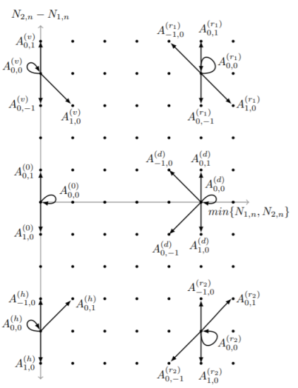
For reasons that will become clear in the following sections, we consider the corresponding uniformized discrete time Markov chain through the uniformization technique. Since the total transition rate from each state is bounded by λ+μ+α1+α2𝜆𝜇subscript𝛼1subscript𝛼2\lambda+\mu+\alpha_{1}+\alpha_{2}, we can construct by uniformization a discrete time Markov chain with the same stationary distribution as that of {X(t);t0}𝑋𝑡𝑡0\{X(t);t\geq 0\}. Without loss of generality, let the uniformization parameter θ=λ+μ+α1+α2=1𝜃𝜆𝜇subscript𝛼1subscript𝛼21\theta=\lambda+\mu+\alpha_{1}+\alpha_{2}=1. The uniformized Markov chain X(n)={(N1,n,N2,n,Cn)}𝑋𝑛subscript𝑁1𝑛subscript𝑁2𝑛subscript𝐶𝑛X(n)=\{(N_{1,n},N_{2,n},C_{n})\} of {X(t);t0}𝑋𝑡𝑡0\{X(t);t\geq 0\} has six regions of spatial homogeneity: two angles, say r1={i>j>0,k=0,1}r_{1}=\{i>j>0,k=0,1\} and r2={j>i>0,k=0,1}r_{2}=\{j>i>0,k=0,1\}, three rays, say h={j=0,i>0,k=0,1}formulae-sequence𝑗0formulae-sequence𝑖0𝑘01h=\{j=0,i>0,k=0,1\}, v={i=0,j>0,k=0,1}𝑣formulae-sequence𝑖0formulae-sequence𝑗0𝑘01v=\{i=0,j>0,k=0,1\}, d={i=j>0,k=0,1}d=\{i=j>0,k=0,1\} and the points {(0,0,k),k=0,1}formulae-sequence00𝑘𝑘01\{(0,0,k),k=0,1\}. Then, the matrix transition diagram partitioned according to the state of the server, is depicted in Figure 1, where
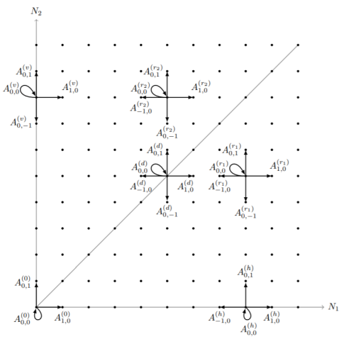
A1,0(r1)=(000λ1)=A1,0(h)=A1,0(0),A1,0(r2)=(000λ1+λ0)=A1,0(v),A1,0(d)=(000λ1+λ0/2),A0,1(r2)=(000λ2)=A0,1(v)=A0,1(0),A0,1(r1)=(000λ0+λ2)=A0,1(h),A0,1(d)=(000λ0/2+λ2),A0,1(r2)=(0α200)=A0,1(v)=A0,1(d)=A0,1(r1),A0,0(v)=(μ+α1λμα1+α2),A1,0(r1)=(0α100)=A1,0(h)=A1,0(d)=A1,0(r2),A0,0(h)=(μ+α2λμα1+α2),A0,0(r1)=(μλμα1+α2)=A0,0(r2)=A0,0(d),A0,0(0)=(μ+α1+α2λμα1+α2).formulae-sequencesuperscriptsubscript𝐴10subscript𝑟1matrix000subscript𝜆1superscriptsubscript𝐴10superscriptsubscript𝐴100superscriptsubscript𝐴10subscript𝑟2matrix000subscript𝜆1subscript𝜆0superscriptsubscript𝐴10𝑣superscriptsubscript𝐴10𝑑matrix000subscript𝜆1subscript𝜆02formulae-sequencesuperscriptsubscript𝐴01subscript𝑟2matrix000subscript𝜆2superscriptsubscript𝐴01𝑣superscriptsubscript𝐴010superscriptsubscript𝐴01subscript𝑟1matrix000subscript𝜆0subscript𝜆2superscriptsubscript𝐴01superscriptsubscript𝐴01𝑑matrix000subscript𝜆02subscript𝜆2formulae-sequencesuperscriptsubscript𝐴01subscript𝑟2matrix0subscript𝛼200superscriptsubscript𝐴01𝑣superscriptsubscript𝐴01𝑑superscriptsubscript𝐴01subscript𝑟1superscriptsubscript𝐴00𝑣matrix𝜇subscript𝛼1𝜆𝜇subscript𝛼1subscript𝛼2formulae-sequencesuperscriptsubscript𝐴10subscript𝑟1matrix0subscript𝛼100superscriptsubscript𝐴10superscriptsubscript𝐴10𝑑superscriptsubscript𝐴10subscript𝑟2superscriptsubscript𝐴00matrix𝜇subscript𝛼2𝜆𝜇subscript𝛼1subscript𝛼2formulae-sequencesuperscriptsubscript𝐴00subscript𝑟1matrix𝜇𝜆𝜇subscript𝛼1subscript𝛼2superscriptsubscript𝐴00subscript𝑟2superscriptsubscript𝐴00𝑑superscriptsubscript𝐴000matrix𝜇subscript𝛼1subscript𝛼2𝜆𝜇subscript𝛼1subscript𝛼2\begin{array}[]{c}A_{1,0}^{(r_{1})}=\begin{pmatrix}0&0\\ 0&\lambda_{1}\end{pmatrix}=A_{1,0}^{(h)}=A_{1,0}^{(0)},\,A_{1,0}^{(r_{2})}=\begin{pmatrix}0&0\\ 0&\lambda_{1}+\lambda_{0}\end{pmatrix}=A_{1,0}^{(v)},\,\,A_{1,0}^{(d)}=\begin{pmatrix}0&0\\ 0&\lambda_{1}+\lambda_{0}/2\end{pmatrix},\\ A_{0,1}^{(r_{2})}=\begin{pmatrix}0&0\\ 0&\lambda_{2}\end{pmatrix}=A_{0,1}^{(v)}=A_{0,1}^{(0)},\,A_{0,1}^{(r_{1})}=\begin{pmatrix}0&0\\ 0&\lambda_{0}+\lambda_{2}\end{pmatrix}=A_{0,1}^{(h)},\,A_{0,1}^{(d)}=\begin{pmatrix}0&0\\ 0&\lambda_{0}/2+\lambda_{2}\end{pmatrix},\\ A_{0,-1}^{(r_{2})}=\begin{pmatrix}0&\alpha_{2}\\ 0&0\end{pmatrix}=A_{0,-1}^{(v)}=A_{0,-1}^{(d)}=A_{0,-1}^{(r_{1})},\,A_{0,0}^{(v)}=\begin{pmatrix}\mu+\alpha_{1}&\lambda\\ \mu&\alpha_{1}+\alpha_{2}\end{pmatrix},\\ A_{-1,0}^{(r_{1})}=\begin{pmatrix}0&\alpha_{1}\\ 0&0\end{pmatrix}=A_{-1,0}^{(h)}=A_{-1,0}^{(d)}=A_{-1,0}^{(r_{2})},\,A_{0,0}^{(h)}=\begin{pmatrix}\mu+\alpha_{2}&\lambda\\ \mu&\alpha_{1}+\alpha_{2}\end{pmatrix},\\ A_{0,0}^{(r_{1})}=\begin{pmatrix}\mu&\lambda\\ \mu&\alpha_{1}+\alpha_{2}\end{pmatrix}=A_{0,0}^{(r_{2})}=A_{0,0}^{(d)},\,A_{0,0}^{(0)}=\begin{pmatrix}\mu+\alpha_{1}+\alpha_{2}&\lambda\\ \mu&\alpha_{1}+\alpha_{2}\end{pmatrix}.\end{array}
Refer to caption
Figure 1: Matrix transition diagram.

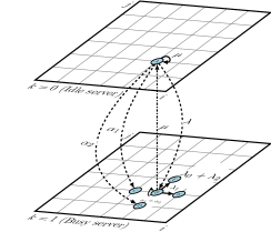
An illustration of the transitions from a state belonging to the angle r1subscript𝑟1r_{1} (e.g., from the state (4,2,k)42𝑘(4,2,k), k=0,1𝑘01k=0,1), and from a state belonging to the ray d𝑑d (e.g., from the state (3,3,k)33𝑘(3,3,k), k=0,1𝑘01k=0,1), is given in Figure 2, left and right, respectively.
Refer to caption
Refer to caption
Figure 2: An instance of state transitions from states belonging to angle r1subscript𝑟1r_{1} (left), and ray d𝑑d (right), given the state of the server.

Lets say some more words regarding the derivation of Ai,j(q)superscriptsubscript𝐴𝑖𝑗𝑞A_{i,j}^{(q)}, 1i,j1formulae-sequence1𝑖𝑗1-1\leq i,j\leq 1, q=r1,r2,h,v,0𝑞subscript𝑟1subscript𝑟2𝑣0q=r_{1},r_{2},h,v,0. For example, A1,0(r1)superscriptsubscript𝐴10subscript𝑟1A_{1,0}^{(r_{1})} contains the transition probabilities from a state that belongs to the angle r1subscript𝑟1r_{1} and results in an increase by one at the orbit queue 1, i.e., from (i,j,k)𝑖𝑗𝑘(i,j,k) to (i+1,j,l)𝑖1𝑗𝑙(i+1,j,l), where i>j𝑖𝑗i>j, k,l=0,1formulae-sequence𝑘𝑙01k,l=0,1. Clearly, such a transition occurs only when we have a dedicated arrival of type 1, and the server is busy. Similarly, given a state in the ray d𝑑d, A1,0(d)superscriptsubscript𝐴10𝑑A_{1,0}^{(d)} contains transition probabilities that result in an increase by one at orbit queue 1, given that both orbits have the same occupancy. Such a transition is done either with the arrival of a dedicated job, or with the arrival of a smart job who sees both orbits with the same number of jobs and is routed with probability 1/2121/2 to orbit queue 1. The rest of Ai,j(q)superscriptsubscript𝐴𝑖𝑗𝑞A_{i,j}^{(q)}, 1i,j1formulae-sequence1𝑖𝑗1-1\leq i,j\leq 1, q=r1,r2,h,v,0𝑞subscript𝑟1subscript𝑟2𝑣0q=r_{1},r_{2},h,v,0, are constructed similarly.

In the following sections, we provide our main results that refer to the asymptotic behaviour of {X(t);t0}𝑋𝑡𝑡0\{X(t);t\geq 0\}. We first investigate the stability conditions. Then, our first main result refers to the investigation of the decay rate of the tail probabilities for the shortest queue length in steady state; see Theorem 4.1. We cope with this task in a number of steps, after considering the corresponding discrete time Markov chain {X(n);n0}𝑋𝑛𝑛0\{X(n);n\geq 0\} through the uniformization technique:

  1. 1.

    We transform the uniformized Markov chain to create the minimum and the difference of the queue states process (i.e., the Markov modulated random walk in the half-plane), and then consider the censored process at busy states.

  2. 2.

    We investigate the stationary tail decay rate of the censored process at busy states.

  3. 3.

    Using a relation among busy and idle states, we show that the asymptotic properties of the shortest queue for the idle states is the same with its asymptotic properties for the busy states.

Our second main result relies on a heuristic approach to construct approximations for the stationary distribution of the original process. In particular, our aim (see Lemmas 2, 3) is to solve (2.1)-(2.7) as either i𝑖i or j𝑗j\to\infty. This task is accomplished by constructing a solution of (2.1)-(2.7) separately in each of the regions defined as follows: Region I: i1much-greater-than𝑖1i\gg 1, j1much-greater-than𝑗1j\gg 1, Region II: i=0𝑖0i=0 or 111, j1much-greater-than𝑗1j\gg 1, Region III: i1much-greater-than𝑖1i\gg 1, j=0𝑗0j=0 or 111.

3 On the stability condition

In this section, we investigate the stability condition of the model at hand. Stability condition for the standard generalized join the shortest queue (GJSQ) model without retrials was recently investigated; see e.g., [15, 24]. Clearly, the presence of retrials along with the presence of the dedicated arrival flows to each orbit when the server is busy, complicates the problem considerably. Note that our model is described by a non-homogeneous Markov modulated two-dimensional nearest-neighbour random walk, and its stability condition, to our best knowledge, is still an open problem. We mention here that the stability condition of a homogeneous Markov modulated two-dimensional nearest neighbour random walk was recently investigated in [34] by using the concept of induced Markov chains.

Here on, by noting that the orbit queues grow only when the server is busy, we construct a new discrete time Markov chain embedded at epochs in which the server is busy, i.e., the censored Markov chain at busy states (censored Markov chains have been widely used for proving the uniqueness of the stationary vector for a recurrent countable-state Markov chain [20, 43]). Then, using standard Foster-Lyapunov arguments, we provide its stability conditions, and having in mind that orbits grow only when the server is busy (it is natural to assume that the behaviour of the original process at the busy states heavily affects its convergence), we conjecture that the obtained stability conditions for the censored Markov chain on the busy states coincides with those of the original one. Simulation experiments indicate that our conjecture is true. The formal justification of our conjecture is an interesting open problem and we let it be a future study.

We first consider the uniformized discrete time Markov chain, say X(n)={(N1,n,N2,n,Cn);n0}𝑋𝑛subscript𝑁1𝑛subscript𝑁2𝑛subscript𝐶𝑛𝑛0X(n)=\{(N_{1,n},N_{2,n},C_{n});n\geq 0\}, of {X(t);t0}𝑋𝑡𝑡0\{X(t);t\geq 0\} with transition diagram given in (1) and state space S=EE~𝑆𝐸~𝐸S=E\cup\tilde{E}, where E=0×0×{1}𝐸subscript0subscript01E=\mathbb{N}_{0}\times\mathbb{N}_{0}\times\{1\}, Ec=0×0×{0}superscript𝐸𝑐subscript0subscript00E^{c}=\mathbb{N}_{0}\times\mathbb{N}_{0}\times\{0\}. Then, we partition the transition matrix P𝑃P of X(n)𝑋𝑛X(n) according to E𝐸E, Ecsuperscript𝐸𝑐E^{c} into:

P=EcEEc( P0,0P0,1) EP1,0P1,1,P=\bordermatrix{&E^{c}&E\cr E^{c}&P_{0,0}&P_{0,1}\cr E&P_{1,0}&P_{1,1}},

where

P0,0=diag(A0,A1,A1,),P1,0=diag(L0,L0,L0,),P0,1=(B0B1B0B1B0),P1,1=(D0,0D0,1D1,1D1,2D2,2D2,3),A0=diag(μ+α1+α2,μ+α1,μ+α1,),A1=diag(μ+α2,μ,μ,),L0=μI,B1=α1I,B0=(λα2λα2λ),Di,i=(α1+α2)I+Qi+1,i+2,i=0,1,,subscript𝑃00𝑑𝑖𝑎𝑔subscript𝐴0subscript𝐴1subscript𝐴1subscript𝑃10𝑑𝑖𝑎𝑔subscript𝐿0subscript𝐿0subscript𝐿0subscript𝑃01matrixsubscript𝐵0missing-subexpressionmissing-subexpressionmissing-subexpressionmissing-subexpressionsubscript𝐵1subscript𝐵0missing-subexpressionmissing-subexpressionmissing-subexpressionmissing-subexpressionsubscript𝐵1subscript𝐵0missing-subexpressionmissing-subexpressionmissing-subexpressionmissing-subexpressionmissing-subexpressionsubscript𝑃11matrixsubscript𝐷00subscript𝐷01missing-subexpressionmissing-subexpressionmissing-subexpressionmissing-subexpressionsubscript𝐷11subscript𝐷12missing-subexpressionmissing-subexpressionmissing-subexpressionmissing-subexpressionsubscript𝐷22subscript𝐷23missing-subexpressionmissing-subexpressionmissing-subexpressionmissing-subexpressionsubscript𝐴0𝑑𝑖𝑎𝑔𝜇subscript𝛼1subscript𝛼2𝜇subscript𝛼1𝜇subscript𝛼1subscript𝐴1𝑑𝑖𝑎𝑔𝜇subscript𝛼2𝜇𝜇subscript𝐿0𝜇subscript𝐼subscript𝐵1subscript𝛼1subscript𝐼subscript𝐵0matrix𝜆missing-subexpressionmissing-subexpressionmissing-subexpressionmissing-subexpressionsubscript𝛼2𝜆missing-subexpressionmissing-subexpressionmissing-subexpressionmissing-subexpressionsubscript𝛼2𝜆missing-subexpressionmissing-subexpressionmissing-subexpressionmissing-subexpressionmissing-subexpressionformulae-sequencesubscript𝐷𝑖𝑖subscript𝛼1subscript𝛼2subscript𝐼subscript𝑄𝑖1𝑖2𝑖01\begin{array}[]{rl}P_{0,0}=diag(A_{0},A_{1},A_{1},\ldots),&P_{1,0}=diag(L_{0},L_{0},L_{0},\ldots),\\ P_{0,1}=\begin{pmatrix}B_{0}&&&&\\ B_{1}&B_{0}&&&\\ &B_{1}&B_{0}&&\\ &&\ddots&\ddots&\end{pmatrix},&P_{1,1}=\begin{pmatrix}D_{0,0}&D_{0,1}&&&\\ &D_{1,1}&D_{1,2}&&\\ &&D_{2,2}&D_{2,3}&\\ &&&\ddots&\ddots\end{pmatrix},\\ A_{0}=diag(\mu+\alpha_{1}+\alpha_{2},\mu+\alpha_{1},\mu+\alpha_{1},\ldots),&A_{1}=diag(\mu+\alpha_{2},\mu,\mu,\ldots),\\ L_{0}=\mu I_{\infty},&B_{1}=\alpha_{1}I_{\infty},\\ B_{0}=\begin{pmatrix}\lambda&&&&\\ \alpha_{2}&\lambda&&&\\ &\alpha_{2}&\lambda&&\\ &&\ddots&\ddots&\end{pmatrix},&D_{i,i}=(\alpha_{1}+\alpha_{2})I_{\infty}+Q_{i+1,i+2},\,i=0,1,\ldots,\end{array}

where Isubscript𝐼I_{\infty} is the identity matrix of infinite dimension and Qi+1,i+2subscript𝑄𝑖1𝑖2Q_{i+1,i+2} is a infinite dimension matrix with only non-zero entries at the superdiagonal and such that the (k,k+1)limit-from𝑘𝑘1(k,k+1)-entry equal to λ0+λ2subscript𝜆0subscript𝜆2\lambda_{0}+\lambda_{2}, k=1,2,,i𝑘12𝑖k=1,2,\ldots,i, the (i+1,i+2)limit-from𝑖1𝑖2(i+1,i+2)-entry equals λ02+λ2subscript𝜆02subscript𝜆2\frac{\lambda_{0}}{2}+\lambda_{2}, and the (i+k,i+k+1)limit-from𝑖𝑘𝑖𝑘1(i+k,i+k+1)-entry equals λ2subscript𝜆2\lambda_{2}, k=2,3,𝑘23k=2,3,\ldots. Finally, the matrix Di,i+1subscript𝐷𝑖𝑖1D_{i,i+1}, i=0,1,𝑖01i=0,1,\ldots is a diagonal matrix of infinite dimension with (k,k)limit-from𝑘𝑘(k,k)-entry equal to λ1subscript𝜆1\lambda_{1}, k=1,2,,i𝑘12𝑖k=1,2,\ldots,i, the (i+1,i+1)limit-from𝑖1𝑖1(i+1,i+1)-entry equals λ02+λ1subscript𝜆02subscript𝜆1\frac{\lambda_{0}}{2}+\lambda_{1}, and the (i+k,i+k)limit-from𝑖𝑘𝑖𝑘(i+k,i+k)-entry equals λ0+λ1subscript𝜆0subscript𝜆1\lambda_{0}+\lambda_{1}, k=2,3,𝑘23k=2,3,\ldots. In what follows, denote λ^:=λ(λ+α1+α2)assign^𝜆𝜆𝜆subscript𝛼1subscript𝛼2\widehat{\lambda}:=\lambda(\lambda+\alpha_{1}+\alpha_{2}), λ^k:=λk(λ+α1+α2)assignsubscript^𝜆𝑘subscript𝜆𝑘𝜆subscript𝛼1subscript𝛼2\widehat{\lambda}_{k}:=\lambda_{k}(\lambda+\alpha_{1}+\alpha_{2}), k=0,1,2,𝑘012k=0,1,2, and μ^k=μαksubscript^𝜇𝑘𝜇subscript𝛼𝑘\widehat{\mu}_{k}=\mu\alpha_{k}, k=1,2𝑘12k=1,2.

Since P0,0subscript𝑃00P_{0,0} is a diagonal matrix, its fundamental matrix, say P~0,0subscript~𝑃00\tilde{P}_{0,0} has the form

P~0,0=n=0P0,0n=diag(A~0,A~1,A~1),A~0=diag(1λ,1λ+α2,1λ+α2,)A~1=diag(1λ+α1,1λ+α1+α2,1λα1+α2,).subscript~𝑃00absentsuperscriptsubscript𝑛0superscriptsubscript𝑃00𝑛𝑑𝑖𝑎𝑔subscript~𝐴0subscript~𝐴1subscript~𝐴1subscript~𝐴0absent𝑑𝑖𝑎𝑔1𝜆1𝜆subscript𝛼21𝜆subscript𝛼2subscript~𝐴1absent𝑑𝑖𝑎𝑔1𝜆subscript𝛼11𝜆subscript𝛼1subscript𝛼21𝜆subscript𝛼1subscript𝛼2\begin{array}[]{rl}\tilde{P}_{0,0}=&\sum_{n=0}^{\infty}P_{0,0}^{n}=diag(\tilde{A}_{0},\tilde{A}_{1},\tilde{A}_{1}),\\ \tilde{A}_{0}=&diag(\frac{1}{\lambda},\frac{1}{\lambda+\alpha_{2}},\frac{1}{\lambda+\alpha_{2}},\ldots)\\ \tilde{A}_{1}=&diag(\frac{1}{\lambda+\alpha_{1}},\frac{1}{\lambda+\alpha_{1}+\alpha_{2}},\frac{1}{\lambda\alpha_{1}+\alpha_{2}},\ldots).\end{array}

The censored chain {X~(n);n0}~𝑋𝑛𝑛0\{\tilde{X}(n);n\geq 0\} at busy states has six regions of spatial homogeneity: two angles, say r1={i>j>0}subscript𝑟1𝑖𝑗0r_{1}=\{i>j>0\} and r2={j>i>0}subscript𝑟2𝑗𝑖0r_{2}=\{j>i>0\}, three rays, say h={j=0,i>0}formulae-sequence𝑗0𝑖0h=\{j=0,i>0\}, v={i=0,j>0}𝑣formulae-sequence𝑖0𝑗0v=\{i=0,j>0\}, d={i=j>0}𝑑𝑖𝑗0d=\{i=j>0\} and the point (0,0)00(0,0). Then, the one step transition probability matrix of the censored chain {X~(n);n0}~𝑋𝑛𝑛0\{\tilde{X}(n);n\geq 0\}, given by P(E)=P1,1+P1,0P~0,0P0,1superscript𝑃𝐸subscript𝑃11subscript𝑃10subscript~𝑃00subscript𝑃01P^{(E)}=P_{1,1}+P_{1,0}\tilde{P}_{0,0}P_{0,1} is as follows:

  • In region i>j>0𝑖𝑗0i>j>0 (labelled as r1subscript𝑟1r_{1}),

    p1,0(r1)=λ1,p0,1(r1)=λ0+λ2,p1,0(r1)=μ^1λ+α1+α2,p0,1(r1)=μ^2λ+α1+α2,p0,0(r1)=α1+α2+λμλ+α1+α2,formulae-sequencesuperscriptsubscript𝑝10subscript𝑟1subscript𝜆1formulae-sequencesuperscriptsubscript𝑝01subscript𝑟1subscript𝜆0subscript𝜆2formulae-sequencesuperscriptsubscript𝑝10subscript𝑟1subscript^𝜇1𝜆subscript𝛼1subscript𝛼2formulae-sequencesuperscriptsubscript𝑝01subscript𝑟1subscript^𝜇2𝜆subscript𝛼1subscript𝛼2superscriptsubscript𝑝00subscript𝑟1subscript𝛼1subscript𝛼2𝜆𝜇𝜆subscript𝛼1subscript𝛼2\begin{array}[]{c}p_{1,0}^{(r_{1})}=\lambda_{1},p_{0,1}^{(r_{1})}=\lambda_{0}+\lambda_{2},p_{-1,0}^{(r_{1})}=\frac{\widehat{\mu}_{1}}{\lambda+\alpha_{1}+\alpha_{2}},p_{0,-1}^{(r_{1})}=\frac{\widehat{\mu}_{2}}{\lambda+\alpha_{1}+\alpha_{2}},p_{0,0}^{(r_{1})}=\alpha_{1}+\alpha_{2}+\frac{\lambda\mu}{\lambda+\alpha_{1}+\alpha_{2}},\end{array}
  • In region j>i>0𝑗𝑖0j>i>0 (labelled as r2subscript𝑟2r_{2}),

    p1,0(r2)=λ0+λ1,p0,1(r2)=λ2,p1,0(r2)=μ^1λ+α1+α2,p0,1(r2)=μ^2λ+α1+α2,p0,0(r2)=α1+α2+λμλ+α1+α2,formulae-sequencesuperscriptsubscript𝑝10subscript𝑟2subscript𝜆0subscript𝜆1formulae-sequencesuperscriptsubscript𝑝01subscript𝑟2subscript𝜆2formulae-sequencesuperscriptsubscript𝑝10subscript𝑟2subscript^𝜇1𝜆subscript𝛼1subscript𝛼2formulae-sequencesuperscriptsubscript𝑝01subscript𝑟2subscript^𝜇2𝜆subscript𝛼1subscript𝛼2superscriptsubscript𝑝00subscript𝑟2subscript𝛼1subscript𝛼2𝜆𝜇𝜆subscript𝛼1subscript𝛼2\begin{array}[]{c}p_{1,0}^{(r_{2})}=\lambda_{0}+\lambda_{1},p_{0,1}^{(r_{2})}=\lambda_{2},p_{-1,0}^{(r_{2})}=\frac{\widehat{\mu}_{1}}{\lambda+\alpha_{1}+\alpha_{2}},p_{0,-1}^{(r_{2})}=\frac{\widehat{\mu}_{2}}{\lambda+\alpha_{1}+\alpha_{2}},p_{0,0}^{(r_{2})}=\alpha_{1}+\alpha_{2}+\frac{\lambda\mu}{\lambda+\alpha_{1}+\alpha_{2}},\end{array}
  • In region i=j>0𝑖𝑗0i=j>0 (labelled as d𝑑d),

    p1,0(d)=λ02+λ1,p0,1(d)=λ02+λ2,p1,0(d)=μ^1λ+α1+α2,p0,1(d)=μ^2λ+α1+α2,p0,0(d)=α1+α2+λμλ+α1+α2,formulae-sequencesuperscriptsubscript𝑝10𝑑subscript𝜆02subscript𝜆1formulae-sequencesuperscriptsubscript𝑝01𝑑subscript𝜆02subscript𝜆2formulae-sequencesuperscriptsubscript𝑝10𝑑subscript^𝜇1𝜆subscript𝛼1subscript𝛼2formulae-sequencesuperscriptsubscript𝑝01𝑑subscript^𝜇2𝜆subscript𝛼1subscript𝛼2superscriptsubscript𝑝00𝑑subscript𝛼1subscript𝛼2𝜆𝜇𝜆subscript𝛼1subscript𝛼2\begin{array}[]{c}p_{1,0}^{(d)}=\frac{\lambda_{0}}{2}+\lambda_{1},p_{0,1}^{(d)}=\frac{\lambda_{0}}{2}+\lambda_{2},p_{-1,0}^{(d)}=\frac{\widehat{\mu}_{1}}{\lambda+\alpha_{1}+\alpha_{2}},p_{0,-1}^{(d)}=\frac{\widehat{\mu}_{2}}{\lambda+\alpha_{1}+\alpha_{2}},p_{0,0}^{(d)}=\alpha_{1}+\alpha_{2}+\frac{\lambda\mu}{\lambda+\alpha_{1}+\alpha_{2}},\end{array}
  • In region i=0𝑖0i=0, j>0𝑗0j>0 (labelled as v𝑣v),

    p1,0(v)=λ0+λ1,p0,1(v)=λ2,p0,1(v)=μ^2λ+α2,p0,0(v)=α1+α2+λμλ+α2,formulae-sequencesuperscriptsubscript𝑝10𝑣subscript𝜆0subscript𝜆1formulae-sequencesuperscriptsubscript𝑝01𝑣subscript𝜆2formulae-sequencesuperscriptsubscript𝑝01𝑣subscript^𝜇2𝜆subscript𝛼2superscriptsubscript𝑝00𝑣subscript𝛼1subscript𝛼2𝜆𝜇𝜆subscript𝛼2\begin{array}[]{c}p_{1,0}^{(v)}=\lambda_{0}+\lambda_{1},p_{0,1}^{(v)}=\lambda_{2},p_{0,-1}^{(v)}=\frac{\widehat{\mu}_{2}}{\lambda+\alpha_{2}},p_{0,0}^{(v)}=\alpha_{1}+\alpha_{2}+\frac{\lambda\mu}{\lambda+\alpha_{2}},\end{array}
  • In region j=0𝑗0j=0, i>0𝑖0i>0 (labelled as hh),

    p1,0(h)=λ1,p0,1(h)=λ0+λ2,p1,0(h)=μ^1λ+α1,p0,0(h)=α1+α2+λμλ+α1,formulae-sequencesuperscriptsubscript𝑝10subscript𝜆1formulae-sequencesuperscriptsubscript𝑝01subscript𝜆0subscript𝜆2formulae-sequencesuperscriptsubscript𝑝10subscript^𝜇1𝜆subscript𝛼1superscriptsubscript𝑝00subscript𝛼1subscript𝛼2𝜆𝜇𝜆subscript𝛼1\begin{array}[]{c}p_{1,0}^{(h)}=\lambda_{1},p_{0,1}^{(h)}=\lambda_{0}+\lambda_{2},p_{-1,0}^{(h)}=\frac{\widehat{\mu}_{1}}{\lambda+\alpha_{1}},p_{0,0}^{(h)}=\alpha_{1}+\alpha_{2}+\frac{\lambda\mu}{\lambda+\alpha_{1}},\end{array}
  • For i=j=0𝑖𝑗0i=j=0 (labelled as O𝑂O),

    p1,0(O)=λ1+λ02,p0,1(O)=+λ02+λ2,p0,0(O)=α1+α2+μ.formulae-sequencesuperscriptsubscript𝑝10𝑂subscript𝜆1subscript𝜆02formulae-sequencesuperscriptsubscript𝑝01𝑂subscript𝜆02subscript𝜆2superscriptsubscript𝑝00𝑂subscript𝛼1subscript𝛼2𝜇\begin{array}[]{c}p_{1,0}^{(O)}=\lambda_{1}+\frac{\lambda_{0}}{2},p_{0,1}^{(O)}=+\frac{\lambda_{0}}{2}+\lambda_{2},p_{0,0}^{(O)}=\alpha_{1}+\alpha_{2}+\mu.\end{array}
Remark 1.

Note that the censored chain {X~(n);n0}~𝑋𝑛𝑛0\{\tilde{X}(n);n\geq 0\} describes a new discrete time queueing system consisting of two parallel coupled queues with three job arrival streams, where one of them joins the shortest queue, and the other two are dedicated to each queue. The coupling feature of the two queues is easily realised by noting that e.g., p1,0(h)=μ^2λ+α1>μ^2λ+α1+α2=p1,0(r2)superscriptsubscript𝑝10subscript^𝜇2𝜆subscript𝛼1subscript^𝜇2𝜆subscript𝛼1subscript𝛼2superscriptsubscript𝑝10subscript𝑟2p_{-1,0}^{(h)}=\frac{\widehat{\mu}_{2}}{\lambda+\alpha_{1}}>\frac{\widehat{\mu}_{2}}{\lambda+\alpha_{1}+\alpha_{2}}=p_{-1,0}^{(r_{2})}. The combination of the JSQ feature, along with the coupled processors feature considerably complicates the analysis.

Lemma 1.

The censored chain {X~(n);n0}~𝑋𝑛𝑛0\{\tilde{X}(n);n\geq 0\} is positive recurrent if and only if one of the following conditions hold:

  1. 1.

    ρ1:=λ^1μ^1<1assignsubscript𝜌1subscript^𝜆1subscript^𝜇11\rho_{1}:=\frac{\widehat{\lambda}_{1}}{\widehat{\mu}_{1}}<1, ρ2:=λ^2μ^2<1assignsubscript𝜌2subscript^𝜆2subscript^𝜇21\rho_{2}:=\frac{\widehat{\lambda}_{2}}{\widehat{\mu}_{2}}<1, ρ=λ^μ^1+μ^2<1𝜌^𝜆subscript^𝜇1subscript^𝜇21\rho=\frac{\widehat{\lambda}}{\widehat{\mu}_{1}+\widehat{\mu}_{2}}<1,

  2. 2.

    ρ11subscript𝜌11\rho_{1}\geq 1, f1:=λ(λ1+α1)μ^11<0assignsubscript𝑓1𝜆subscript𝜆1subscript𝛼1subscript^𝜇110f_{1}:=\frac{\lambda(\lambda_{1}+\alpha_{1})}{\widehat{\mu}_{1}}-1<0,

  3. 3.

    ρ21subscript𝜌21\rho_{2}\geq 1, f2:=λ(λ2+α2)μ^21<0assignsubscript𝑓2𝜆subscript𝜆2subscript𝛼2subscript^𝜇210f_{2}:=\frac{\lambda(\lambda_{2}+\alpha_{2})}{\widehat{\mu}_{2}}-1<0.

Proof.

The proof is given in Appendix A. ∎

We now study the dynamics of the orbits in the original process {X(t);t0}𝑋𝑡𝑡0\{X(t);t\geq 0\} based on the stability criteria of the censored process {X~(n);n0}~𝑋𝑛𝑛0\{\tilde{X}(n);n\geq 0\} given in Lemma 1.

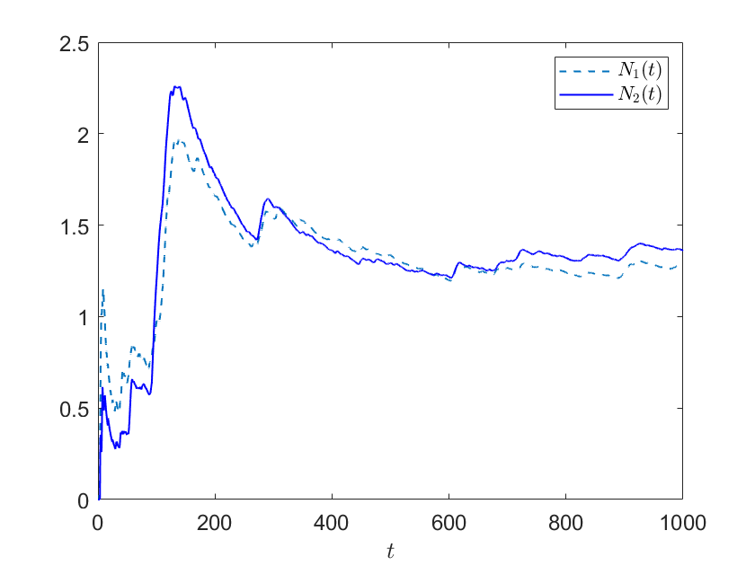
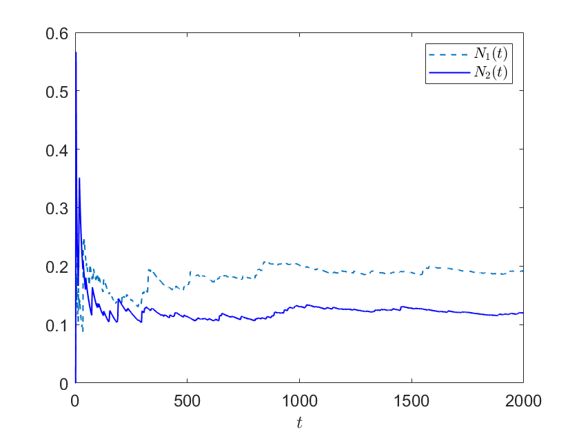
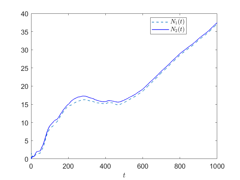
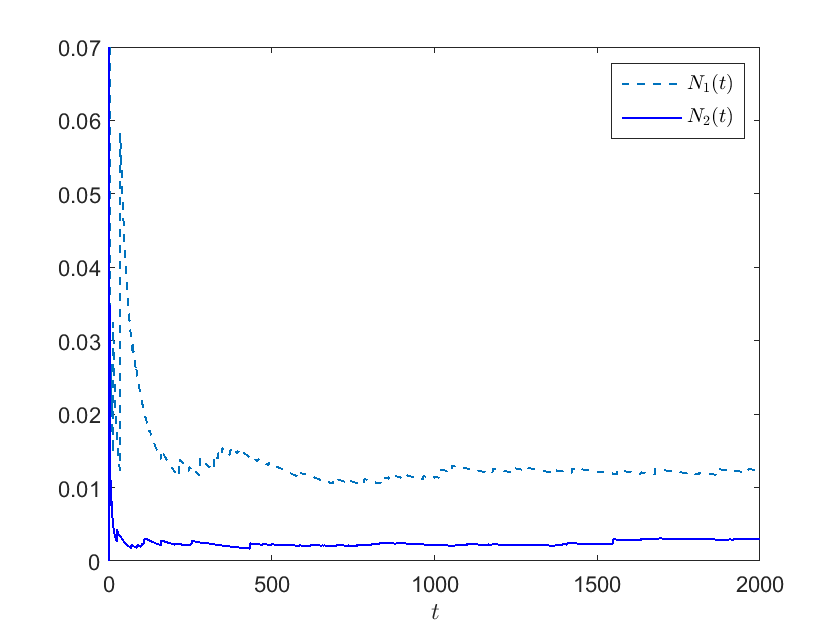
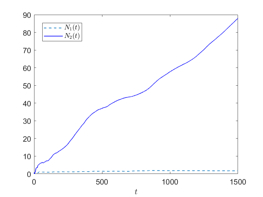
Figure 3 refers to the stability criteria 1. In Figure 3 (left) we have ρ=0.78>max{ρ1=0.433,ρ2=0.325}𝜌0.78𝑚𝑎𝑥formulae-sequencesubscript𝜌10.433subscript𝜌20.325\rho=0.78>max\{\rho_{1}=0.433,\rho_{2}=0.325\} and λ^0|λ^1λ^2+ρ2(μ^2μ^1)|=19.084>0subscript^𝜆0subscript^𝜆1subscript^𝜆2superscript𝜌2subscript^𝜇2subscript^𝜇119.0840\widehat{\lambda}_{0}-|\widehat{\lambda}_{1}-\widehat{\lambda}_{2}+\rho^{2}(\widehat{\mu}_{2}-\widehat{\mu}_{1})|=19.084>0. It is seen that in such a case the original process is stable, and that both orbits are well balanced. This case corresponds to the strongly pooled case mentioned in [15, Theorem 2], i.e., the proportion of jobs that is routed to the least loaded orbit queue in case the server is busy is large. In Figure 3 (middle), we have the case 1>ρ>max{ρ1,ρ2}1𝜌𝑚𝑎𝑥subscript𝜌1subscript𝜌21>\rho>max\{\rho_{1},\rho_{2}\}, with ρ1>ρ2subscript𝜌1subscript𝜌2\rho_{1}>\rho_{2} but now λ^0|λ^1λ^2+ρ2(μ^2μ^1)|<0subscript^𝜆0subscript^𝜆1subscript^𝜆2superscript𝜌2subscript^𝜇2subscript^𝜇10\widehat{\lambda}_{0}-|\widehat{\lambda}_{1}-\widehat{\lambda}_{2}+\rho^{2}(\widehat{\mu}_{2}-\widehat{\mu}_{1})|<0. The original process is still stable but we can observe that the orbit lengths are not so close any more. This means that the stream that joins the shortest orbit failed to keep the orbit queue lengths close enough to each other. In case ρ>1𝜌1\rho>1 both orbits are unstable, even though ρ1<1subscript𝜌11\rho_{1}<1, ρ2<1subscript𝜌21\rho_{2}<1 (Figure 3 (right)).

Refer to caption
Refer to caption
Refer to caption
Figure 3: Orbit dynamics for case 1>ρ>max{ρ1,ρ2}1𝜌𝑚𝑎𝑥subscript𝜌1subscript𝜌21>\rho>max\{\rho_{1},\rho_{2}\}, λ^0|λ^1λ^2+ρ2(μ^2μ^1)|>0subscript^𝜆0subscript^𝜆1subscript^𝜆2superscript𝜌2subscript^𝜇2subscript^𝜇10\widehat{\lambda}_{0}-|\widehat{\lambda}_{1}-\widehat{\lambda}_{2}+\rho^{2}(\widehat{\mu}_{2}-\widehat{\mu}_{1})|>0 (left), 1>ρ>max{ρ1,ρ2}1𝜌𝑚𝑎𝑥subscript𝜌1subscript𝜌21>\rho>max\{\rho_{1},\rho_{2}\}, λ^0|λ^1λ^2+ρ2(μ^2μ^1)|<0subscript^𝜆0subscript^𝜆1subscript^𝜆2superscript𝜌2subscript^𝜇2subscript^𝜇10\widehat{\lambda}_{0}-|\widehat{\lambda}_{1}-\widehat{\lambda}_{2}+\rho^{2}(\widehat{\mu}_{2}-\widehat{\mu}_{1})|<0 (middle), and for the case ρ>1𝜌1\rho>1, ρ1<1subscript𝜌11\rho_{1}<1, ρ2<1subscript𝜌21\rho_{2}<1 (right).

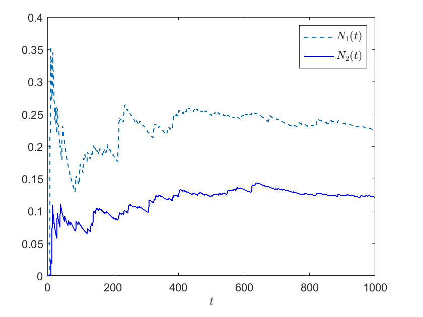
In Figure 4 (left) we have ρ1=0.428>max{ρ=0.4042,ρ2=0.2675}subscript𝜌10.428𝜌0.4042subscript𝜌20.2675\rho_{1}=0.428>\max\{\rho=0.4042,\rho_{2}=0.2675\}, and λ^0|λ^1λ^2+ρ2(μ^2μ^1)|=2.393<0subscript^𝜆0subscript^𝜆1subscript^𝜆2superscript𝜌2subscript^𝜇2subscript^𝜇12.3930\widehat{\lambda}_{0}-|\widehat{\lambda}_{1}-\widehat{\lambda}_{2}+\rho^{2}(\widehat{\mu}_{2}-\widehat{\mu}_{1})|=-2.393<0. In such a case the system is still stable, but the smart stream failed to keep the orbit queue length very close. Similar observations can be also deduced from Figure 4 (right) for which ρ1=0.0944>max{ρ=0.061,ρ2=0.021}subscript𝜌10.0944𝜌0.061subscript𝜌20.021\rho_{1}=0.0944>\max\{\rho=0.061,\rho_{2}=0.021\}, and λ^0|λ^1λ^2+ρ2(μ^2μ^1)|=0.7663>0subscript^𝜆0subscript^𝜆1subscript^𝜆2superscript𝜌2subscript^𝜇2subscript^𝜇10.76630\widehat{\lambda}_{0}-|\widehat{\lambda}_{1}-\widehat{\lambda}_{2}+\rho^{2}(\widehat{\mu}_{2}-\widehat{\mu}_{1})|=0.7663>0.

Refer to caption
Refer to caption
Figure 4: Orbit dynamics for case 1>ρ1>max{ρ,ρ2}1subscript𝜌1𝑚𝑎𝑥𝜌subscript𝜌21>\rho_{1}>max\{\rho,\rho_{2}\}, λ^0|λ^1λ^2+ρ2(μ^2μ^1)|<0subscript^𝜆0subscript^𝜆1subscript^𝜆2superscript𝜌2subscript^𝜇2subscript^𝜇10\widehat{\lambda}_{0}-|\widehat{\lambda}_{1}-\widehat{\lambda}_{2}+\rho^{2}(\widehat{\mu}_{2}-\widehat{\mu}_{1})|<0 (left), 1>ρ1>max{ρ,ρ2}1subscript𝜌1𝑚𝑎𝑥𝜌subscript𝜌21>\rho_{1}>max\{\rho,\rho_{2}\}, λ^0|λ^1λ^2+ρ2(μ^2μ^1)|<0subscript^𝜆0subscript^𝜆1subscript^𝜆2superscript𝜌2subscript^𝜇2subscript^𝜇10\widehat{\lambda}_{0}-|\widehat{\lambda}_{1}-\widehat{\lambda}_{2}+\rho^{2}(\widehat{\mu}_{2}-\widehat{\mu}_{1})|<0 (right).

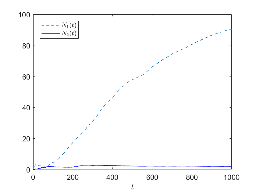
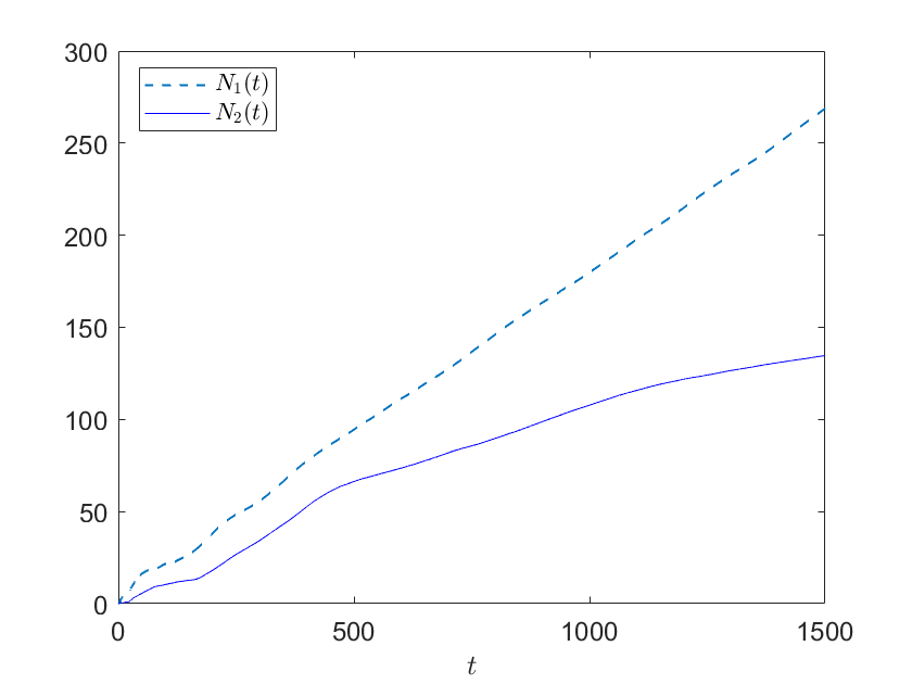
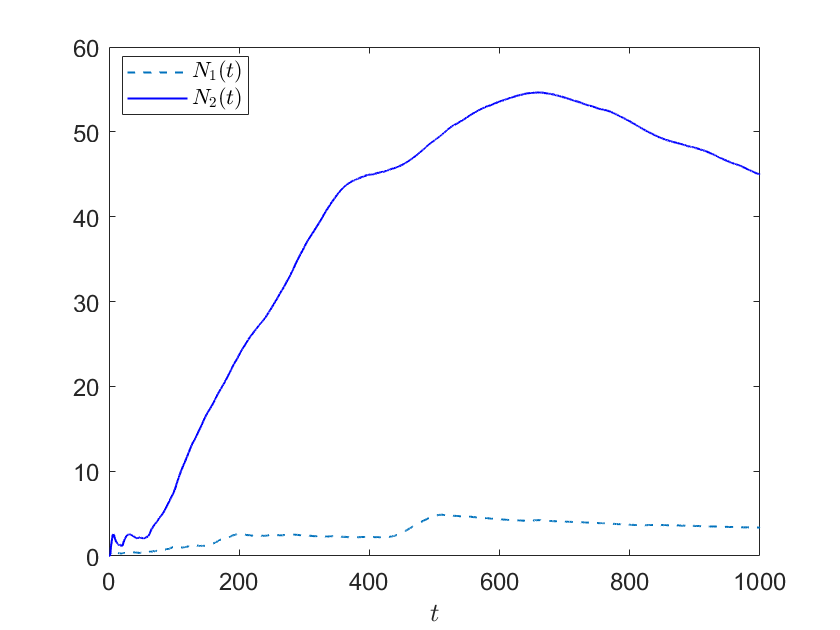
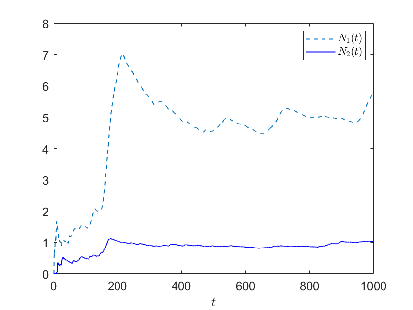
In Figure 5 (left), although ρ1>1subscript𝜌11\rho_{1}>1 (ρ<1𝜌1\rho<1, ρ2<1subscript𝜌21\rho_{2}<1), the fact that f1<0subscript𝑓10f_{1}<0 keeps the network stable. On the other hand when f1>0subscript𝑓10f_{1}>0 (Fig. 5, middle), orbit queue 1 becomes unstable, and so it is the network. Note that in such a case orbit queue 2 remains stable. In Figure 5 (right), when ρ>1𝜌1\rho>1 both orbits becomes unstable, even though ρ2<1subscript𝜌21\rho_{2}<1. Similar observations can be deduced from Figure 6 that refers to the stability criteria 3.
Refer to caption
Refer to caption
Refer to caption
Figure 5: Orbit dynamics for case ρ<1𝜌1\rho<1, ρ1>1subscript𝜌11\rho_{1}>1, ρ2<1subscript𝜌21\rho_{2}<1, f1<0subscript𝑓10f_{1}<0 (left), for the case ρ<1𝜌1\rho<1, ρ1>1subscript𝜌11\rho_{1}>1, ρ2<1subscript𝜌21\rho_{2}<1, f1>0subscript𝑓10f_{1}>0 (middle), and for the case ρ>1𝜌1\rho>1, ρ1>1subscript𝜌11\rho_{1}>1, ρ2<1subscript𝜌21\rho_{2}<1, f1>0subscript𝑓10f_{1}>0 (right).
Refer to caption
Refer to caption
Figure 6: Orbit dynamics for case ρ<1𝜌1\rho<1, ρ1<1subscript𝜌11\rho_{1}<1, ρ2>1subscript𝜌21\rho_{2}>1, f2<0subscript𝑓20f_{2}<0 (left), for the case ρ<1𝜌1\rho<1, ρ1<1subscript𝜌11\rho_{1}<1, ρ2>1subscript𝜌21\rho_{2}>1, f2>0subscript𝑓20f_{2}>0 (right).

Therefore, simulations experiments indicate that the stability criteria given in Lemma 1 constitute stability criteria for the GJSOQ system. A formal justification of this result is postponed in a future work.

4 Main results

4.1 Geometric decay in the minimum direction

In the following, we investigated the tail asymptotic of the stationary distribution of our model provided that ρ1<1subscript𝜌11\rho_{1}<1, ρ2<1subscript𝜌21\rho_{2}<1, ρ<1𝜌1\rho<1. We show that the tail asymptotic for the minimum orbit queue lengths for a fixed value of their difference, and server’s state is exactly geometric. Moreover, we show that its decay rate is the square of the decay rate, i.e., ρ2superscript𝜌2\rho^{2}, of the corresponding modified single orbit queue, say the reference system, which is formally described at the end of this section.

Clearly, when λ1=λ2=0subscript𝜆1subscript𝜆20\lambda_{1}=\lambda_{2}=0, both orbit queues are well balanced by the smart stream, and we again expect that the decay rate of the minimum of orbit queues equals ρ2superscript𝜌2\rho^{2}. Note that this result is motivated by the standard Markovian JSQ model (without retrials), in which the tail decay rate of the minimum of queue lengths is the square of the tail decay rate of the M/M/2. Theorem 4.1 states that our model has a similar behaviour.

Tail asymptotic properties for random walks in the half plane are still very limited including a recent paper by [30], in which the method developed in [29] was extended for studying the standard generalized join the-shortest-queue model. Our goal here is to cope with the tail asymptotic properties of a Markov modulated random walk in the half-plane, with particular interest on a modulation that results in a tractable analysis.

Our approach is summarized in the following steps:

  1. Step 1

    We focus on the uniformized discrete time Markov chain {X(n);n0}𝑋𝑛𝑛0\{X(n);n\geq 0\}, and perform the transformation Z1,n=min{N1,n,N2,n}subscript𝑍1𝑛𝑚𝑖𝑛subscript𝑁1𝑛subscript𝑁2𝑛Z_{1,n}=min\{N_{1,n},N_{2,n}\}, Z2,n=N2,nN1,nsubscript𝑍2𝑛subscript𝑁2𝑛subscript𝑁1𝑛Z_{2,n}=N_{2,n}-N_{1,n}.

  2. Step 2

    The discrete time Markov chain Z(n)={(Z1,n,Z2,n,Cn);n0}𝑍𝑛subscript𝑍1𝑛subscript𝑍2𝑛subscript𝐶𝑛𝑛0Z(n)=\{(Z_{1,n},Z_{2,n},C_{n});n\geq 0\} is a Markov modulated random walk in the half plane with transition diagram as shown in Figure 7, where the matrices Ai,j(m)superscriptsubscript𝐴𝑖𝑗𝑚A_{i,j}^{(m)}, i,j=0,±1formulae-sequence𝑖𝑗0plus-or-minus1i,j=0,\pm 1, m=r1,r2,d,v,h,0𝑚subscript𝑟1subscript𝑟2𝑑𝑣0m=r_{1},r_{2},d,v,h,0 are given in Section 2. Then, we consider the censored Markov chain of {Z(n);n0}𝑍𝑛𝑛0\{Z(n);n\geq 0\} on the busy states, which can be expressed explicitly. This censored Markov chain is a random walk in the half plane.

  3. Step 3

    We investigate the tail asymptotic behaviour of this censored Markov chain at the busy states following [26], and show that the minimum orbit queue length decays geometrically; see Theorem 4.1.

  4. Step 4

    By exploiting a relation between idle and busy states (see (4.5)), we further show that the minimum orbit queue length at the idle states decays also geometrically; see Corollary 1.

Refer to caption
Figure 7: The matrix transition diagram of {Z(n);n0}𝑍𝑛𝑛0\{Z(n);n\geq 0\}.

Note that the presence of dedicated streams that are routed to the shortest orbit in case of a busy server complicates considerably the problem of decay rates. We are also interested in when the two orbit queues are balanced. Intuitively, the two orbit queues being balanced when the smart arrival stream, which routes the job to the least loaded orbit queue, keeps the two orbit queue lengths close. Since the difference of the two orbit queues is the background state, the balancing of the two orbit queues is characterized by how the background process behaves as the level process (i.e., the shortest orbit queue) goes up.

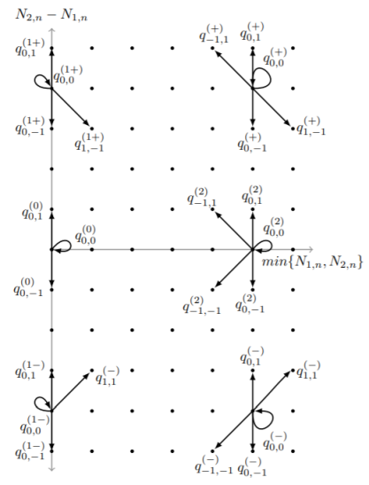
By applying a similar procedure as in Section 3, the censored Markov chain on the busy states of {Z(n);n0}𝑍𝑛𝑛0\{Z(n);n\geq 0\}, is a two-dimensional random walk on the half plane {(m,l)2;l0}formulae-sequence𝑚𝑙superscript2𝑙0\{(m,l)\in\mathbb{Z}^{2};l\geq 0\}, say Y(n)={(Y1,n,Y2,n,1);n0}𝑌𝑛subscript𝑌1𝑛subscript𝑌2𝑛1𝑛0Y(n)=\{(Y_{1,n},Y_{2,n},1);n\geq 0\}, where Y1,n=N2,nN1,nsubscript𝑌1𝑛subscript𝑁2𝑛subscript𝑁1𝑛Y_{1,n}=N_{2,n}-N_{1,n}, Y2,n=min{N1,n,N2,n}subscript𝑌2𝑛𝑚𝑖𝑛subscript𝑁1𝑛subscript𝑁2𝑛Y_{2,n}=min\{N_{1,n},N_{2,n}\}. Its transition rate diagram is given in Figure 8, where its one step transition probabilities are:

q0,1()=λ1,q1,1()=μ^2λ+α1+α2,q0,1()=μ^1λ+α1+α2,q1,1()=λ0+λ2,q0,0()=α1+α2+λμλ+α1+α2,q0,1(+)=λ2,q0,1(+)=μ^2λ+α1+α2,q1,1(+)=μ^1λ+α1+α2,q1,1(+)=λ0+λ1,q0,0(+)=α1+α2+λμλ+α1+α2,q0,1(2)=λ2+λ02,q1,1(2)=μ^2λ+α1+α2,q1,1(2)=μ^1λ+α1+α2,q0,1(2)=λ02+λ1,q0,0(2)=α1+α2+λμλ+α1+α2,q0,1(1)=λ1,q0,1(1)=μ^1λ+α1,q1,1(1)=λ0+λ2,q0,0(1)=α1+α2+λμλ+α1,q0,1(1+)=λ2,q0,1(1+)=μ^2λ+α2,q1,1(1+)=λ0+λ1,q0,0(1+)=α1+α2+λμλ+α2,q0,1(0)=λ2+λ02,q0,0(0)=α1+α2+μ,q0,1(0)=λ1+λ02.formulae-sequencesuperscriptsubscript𝑞01subscript𝜆1formulae-sequencesuperscriptsubscript𝑞11subscript^𝜇2𝜆subscript𝛼1subscript𝛼2formulae-sequencesuperscriptsubscript𝑞01subscript^𝜇1𝜆subscript𝛼1subscript𝛼2formulae-sequencesuperscriptsubscript𝑞11subscript𝜆0subscript𝜆2superscriptsubscript𝑞00subscript𝛼1subscript𝛼2𝜆𝜇𝜆subscript𝛼1subscript𝛼2formulae-sequencesuperscriptsubscript𝑞01subscript𝜆2formulae-sequencesuperscriptsubscript𝑞01subscript^𝜇2𝜆subscript𝛼1subscript𝛼2formulae-sequencesuperscriptsubscript𝑞11subscript^𝜇1𝜆subscript𝛼1subscript𝛼2formulae-sequencesuperscriptsubscript𝑞11subscript𝜆0subscript𝜆1superscriptsubscript𝑞00subscript𝛼1subscript𝛼2𝜆𝜇𝜆subscript𝛼1subscript𝛼2formulae-sequencesuperscriptsubscript𝑞012subscript𝜆2subscript𝜆02formulae-sequencesuperscriptsubscript𝑞112subscript^𝜇2𝜆subscript𝛼1subscript𝛼2formulae-sequencesuperscriptsubscript𝑞112subscript^𝜇1𝜆subscript𝛼1subscript𝛼2formulae-sequencesuperscriptsubscript𝑞012subscript𝜆02subscript𝜆1superscriptsubscript𝑞002subscript𝛼1subscript𝛼2𝜆𝜇𝜆subscript𝛼1subscript𝛼2formulae-sequencesuperscriptsubscript𝑞01limit-from1subscript𝜆1formulae-sequencesuperscriptsubscript𝑞01limit-from1subscript^𝜇1𝜆subscript𝛼1formulae-sequencesuperscriptsubscript𝑞11limit-from1subscript𝜆0subscript𝜆2superscriptsubscript𝑞00limit-from1subscript𝛼1subscript𝛼2𝜆𝜇𝜆subscript𝛼1formulae-sequencesuperscriptsubscript𝑞01limit-from1subscript𝜆2formulae-sequencesuperscriptsubscript𝑞01limit-from1subscript^𝜇2𝜆subscript𝛼2formulae-sequencesuperscriptsubscript𝑞11limit-from1subscript𝜆0subscript𝜆1superscriptsubscript𝑞00limit-from1subscript𝛼1subscript𝛼2𝜆𝜇𝜆subscript𝛼2formulae-sequencesuperscriptsubscript𝑞010subscript𝜆2subscript𝜆02formulae-sequencesuperscriptsubscript𝑞000subscript𝛼1subscript𝛼2𝜇superscriptsubscript𝑞010subscript𝜆1subscript𝜆02\begin{array}[]{c}q_{0,-1}^{(-)}=\lambda_{1},\,q_{-1,-1}^{(-)}=\frac{\widehat{\mu}_{2}}{\lambda+\alpha_{1}+\alpha_{2}},\,q_{0,1}^{(-)}=\frac{\widehat{\mu}_{1}}{\lambda+\alpha_{1}+\alpha_{2}},\,q_{1,1}^{(-)}=\lambda_{0}+\lambda_{2},\,q_{0,0}^{(-)}=\alpha_{1}+\alpha_{2}+\frac{\lambda\mu}{\lambda+\alpha_{1}+\alpha_{2}},\\ q_{0,1}^{(+)}=\lambda_{2},\,q_{0,-1}^{(+)}=\frac{\widehat{\mu}_{2}}{\lambda+\alpha_{1}+\alpha_{2}},\,q_{-1,1}^{(+)}=\frac{\widehat{\mu}_{1}}{\lambda+\alpha_{1}+\alpha_{2}},\,q_{1,-1}^{(+)}=\lambda_{0}+\lambda_{1},\,q_{0,0}^{(+)}=\alpha_{1}+\alpha_{2}+\frac{\lambda\mu}{\lambda+\alpha_{1}+\alpha_{2}},\\ q_{0,1}^{(2)}=\lambda_{2}+\frac{\lambda_{0}}{2},\,q_{-1,-1}^{(2)}=\frac{\widehat{\mu}_{2}}{\lambda+\alpha_{1}+\alpha_{2}},\,q_{-1,1}^{(2)}=\frac{\widehat{\mu}_{1}}{\lambda+\alpha_{1}+\alpha_{2}},\,q_{0,-1}^{(2)}=\frac{\lambda_{0}}{2}+\lambda_{1},\,q_{0,0}^{(2)}=\alpha_{1}+\alpha_{2}+\frac{\lambda\mu}{\lambda+\alpha_{1}+\alpha_{2}},\\ q_{0,-1}^{(1-)}=\lambda_{1},\,q_{0,1}^{(1-)}=\frac{\widehat{\mu}_{1}}{\lambda+\alpha_{1}},\,q_{1,1}^{(1-)}=\lambda_{0}+\lambda_{2},\,q_{0,0}^{(1-)}=\alpha_{1}+\alpha_{2}+\frac{\lambda\mu}{\lambda+\alpha_{1}},\\ q_{0,1}^{(1+)}=\lambda_{2},\,q_{0,-1}^{(1+)}=\frac{\widehat{\mu}_{2}}{\lambda+\alpha_{2}},\,q_{1,-1}^{(1+)}=\lambda_{0}+\lambda_{1},\,q_{0,0}^{(1+)}=\alpha_{1}+\alpha_{2}+\frac{\lambda\mu}{\lambda+\alpha_{2}},\\ q_{0,1}^{(0)}=\lambda_{2}+\frac{\lambda_{0}}{2},\,q_{0,0}^{(0)}=\alpha_{1}+\alpha_{2}+\mu,\,q_{0,-1}^{(0)}=\lambda_{1}+\frac{\lambda_{0}}{2}.\end{array} (4.1)
Refer to caption
Figure 8: Transition rate diagram of the censored chain {Y(n);n0}𝑌𝑛𝑛0\{Y(n);n\geq 0\}.
Remark 2.

Note that {Y(n);n0}𝑌𝑛𝑛0\{Y(n);n\geq 0\} can be also obtained by the censored Markov chain {X~(n);n0}~𝑋𝑛𝑛0\{\tilde{X}(n);n\geq 0\} (on the busy states of {X(n);n0}𝑋𝑛𝑛0\{X(n);n\geq 0\}), by applying the transformation Y1,n=min{N1,n,N2,n}subscript𝑌1𝑛𝑚𝑖𝑛subscript𝑁1𝑛subscript𝑁2𝑛Y_{1,n}=min\{N_{1,n},N_{2,n}\}, Y2,n=N2,nN1,nsubscript𝑌2𝑛subscript𝑁2𝑛subscript𝑁1𝑛Y_{2,n}=N_{2,n}-N_{1,n}.

The main result is summarized in the following theorem. Let 𝝅{𝝅m,m=0,1,}\boldsymbol{\pi}\equiv\{\boldsymbol{\pi}_{m},m=0,1,\ldots\} be the stationary joint distribution of min{N1,n,N2,n}𝑚𝑖𝑛subscript𝑁1𝑛subscript𝑁2𝑛min\{N_{1,n},N_{2,n}\} and N2,nN1,nsubscript𝑁2𝑛subscript𝑁1𝑛N_{2,n}-N_{1,n} when the server is busy, where 𝝅m={πm,l(1),l=0,±1,±2,}\boldsymbol{\pi}_{m}=\{\pi_{m,l}(1),l=0,\pm 1,\pm 2,\ldots\} is the subvector for level m𝑚m, i.e.,

πm,l(1)=limn(min{N1,n,N2,n}=m,N2,nN1,n=l,Cn=1),m0,l.formulae-sequencesubscript𝜋𝑚𝑙1subscript𝑛formulae-sequence𝑚𝑖𝑛subscript𝑁1𝑛subscript𝑁2𝑛𝑚formulae-sequencesubscript𝑁2𝑛subscript𝑁1𝑛𝑙subscript𝐶𝑛1formulae-sequence𝑚0𝑙\begin{array}[]{c}\pi_{m,l}(1)=\lim_{n\to\infty}\mathbb{P}(min\{N_{1,n},N_{2,n}\}=m,N_{2,n}-N_{1,n}=l,C_{n}=1),\,m\geq 0,l\in\mathbb{Z}.\end{array}
Theorem 4.1.

For the generalized join the shortest orbit queue system satisfying max{ρ1,ρ2}<ρ<1𝑚𝑎𝑥subscript𝜌1subscript𝜌2𝜌1max\{\rho_{1},\rho_{2}\}<\rho<1, and λ^0>|λ^2λ^1+ρ2(μ^1μ^2)|subscript^𝜆0subscript^𝜆2subscript^𝜆1superscript𝜌2subscript^𝜇1subscript^𝜇2\widehat{\lambda}_{0}>|\widehat{\lambda}_{2}-\widehat{\lambda}_{1}+\rho^{2}(\widehat{\mu}_{1}-\widehat{\mu}_{2})|, the stationary probability vector 𝛑msubscript𝛑𝑚\boldsymbol{\pi}_{m} decays geometrically as m𝑚m\to\infty with decay rate ρ2superscript𝜌2\rho^{2}, i.e.,

limmρ2mπm,l(1)=xl(ρ2),subscript𝑚superscript𝜌2𝑚subscript𝜋𝑚𝑙1subscript𝑥𝑙superscript𝜌2\lim_{m\to\infty}\rho^{-2m}\pi_{m,l}(1)=x_{l}(\rho^{-2}), (4.2)

where

xl(ρ2)={γ2+λ^0/2γ2x0(ργ2γ1+λ^0)|l|,l1,x0,l=0,γ1+λ^0/2γ1x0(ργ1γ2+λ^0)l,l1,subscript𝑥𝑙superscript𝜌2casessubscript𝛾2subscript^𝜆02subscript𝛾2subscript𝑥0superscript𝜌subscript𝛾2subscript𝛾1subscript^𝜆0𝑙𝑙1subscript𝑥0𝑙0subscript𝛾1subscript^𝜆02subscript𝛾1subscript𝑥0superscript𝜌subscript𝛾1subscript𝛾2subscript^𝜆0𝑙𝑙1missing-subexpression\begin{array}[]{rl}x_{l}(\rho^{-2})=\left\{\begin{array}[]{ll}\frac{\gamma_{2}+\widehat{\lambda}_{0}/2}{\gamma_{2}}x_{0}\left(\rho\frac{\gamma_{2}}{\gamma_{1}+\widehat{\lambda}_{0}}\right)^{|l|},&l\leq-1,\\ x_{0},&l=0,\\ \frac{\gamma_{1}+\widehat{\lambda}_{0}/2}{\gamma_{1}}x_{0}\left(\rho\frac{\gamma_{1}}{\gamma_{2}+\widehat{\lambda}_{0}}\right)^{l},&l\geq 1,\end{array}\right.\end{array} (4.3)

where x0subscript𝑥0x_{0} is a constant and γ1=μ^1ρ2+λ^2subscript𝛾1subscript^𝜇1superscript𝜌2subscript^𝜆2\gamma_{1}=\widehat{\mu}_{1}\rho^{2}+\widehat{\lambda}_{2}, γ2=μ^2ρ2+λ^1subscript𝛾2subscript^𝜇2superscript𝜌2subscript^𝜆1\gamma_{2}=\widehat{\mu}_{2}\rho^{2}+\widehat{\lambda}_{1}. Moreover, the two orbit queues are strongly balanced if and only if γ2<ρ(γ1+λ^0)subscript𝛾2𝜌subscript𝛾1subscript^𝜆0\gamma_{2}<\rho(\gamma_{1}+\widehat{\lambda}_{0}), γ1<ρ(γ2+λ^0)subscript𝛾1𝜌subscript𝛾2subscript^𝜆0\gamma_{1}<\rho(\gamma_{2}+\widehat{\lambda}_{0}).

Proof.

The proof is based on a series of results, and is given in Section 5.1. ∎

Having known the exact tail asymptotic properties for C(t)=1𝐶𝑡1C(t)=1 (i.e., when the server is busy), we can investigate the tail asymptotic properties for C(t)=0𝐶𝑡0C(t)=0 (i.e., when the server is idle) based on the relationship given in (4.5) (which is similar to (2.1)).

Corollary 1.

Based on the relationship given in (4.5),

ρ2mπm,l(0)μλ+α1+α2xl(ρ2),l,formulae-sequencesimilar-tosuperscript𝜌2𝑚subscript𝜋𝑚𝑙0𝜇𝜆subscript𝛼1subscript𝛼2subscript𝑥𝑙superscript𝜌2𝑙\rho^{-2m}\pi_{m,l}(0)\sim\frac{\mu}{\lambda+\alpha_{1}+\alpha_{2}}x_{l}(\rho^{-2}),\,l\in\mathbb{Z}, (4.4)

where xl(ρ2)subscript𝑥𝑙superscript𝜌2x_{l}(\rho^{-2}), l𝑙l\in\mathbb{Z} as given in Theorem 4.1.

Proof.

We consider the Markov chain Z(n)={(Z1,n,Z2,n,Cn);n0}𝑍𝑛subscript𝑍1𝑛subscript𝑍2𝑛subscript𝐶𝑛𝑛0Z(n)=\{(Z_{1,n},Z_{2,n},C_{n});n\geq 0\} where Z1,n=min{N1,n,N2,n}subscript𝑍1𝑛𝑚𝑖𝑛subscript𝑁1𝑛subscript𝑁2𝑛Z_{1,n}=min\{N_{1,n},N_{2,n}\}, Z2,n=N2,nN1,nsubscript𝑍2𝑛subscript𝑁2𝑛subscript𝑁1𝑛Z_{2,n}=N_{2,n}-N_{1,n}; see Figure 7. Knowing the asymptotic properties of πm,l(1)subscript𝜋𝑚𝑙1\pi_{m,l}(1), we will investigate those of πm,l(0)=limn(min{N1,n,N2,n=m},N2,nN1,n=l,Cn=0)\pi_{m,l}(0)=\lim_{n\to\infty}\mathbb{P}(min\{N_{1,n},N_{2,n}=m\},N_{2,n}-N_{1,n}=l,C_{n}=0). Note that the equilibrium equations that deal with the idle states are for m>0𝑚0m>0,

πm,l(0)(λ+α1+α2)=μπm,l(1),l,formulae-sequencesubscript𝜋𝑚𝑙0𝜆subscript𝛼1subscript𝛼2𝜇subscript𝜋𝑚𝑙1𝑙\pi_{m,l}(0)(\lambda+\alpha_{1}+\alpha_{2})=\mu\pi_{m,l}(1),\,l\in\mathbb{Z}, (4.5)

which obviously leads to (4.4). ∎

Therefore, we shown that under the conditions max{ρ1,ρ2}<ρ<1𝑚𝑎𝑥subscript𝜌1subscript𝜌2𝜌1max\{\rho_{1},\rho_{2}\}<\rho<1, |γ1γ2|<λ^0subscript𝛾1subscript𝛾2subscript^𝜆0|\gamma_{1}-\gamma_{2}|<\widehat{\lambda}_{0}, the tail decay rate for the shortest orbit queue in our GJSOQ system equals ρ2superscript𝜌2\rho^{2}. It is easy to see that this is the square of the tail decay rate for the orbit queue length of the reference system mentioned at the beginning of this section. The reference system operates as follows: Jobs arrive according to a Poisson process with rate λ=λ0+λ1+λ2𝜆subscript𝜆0subscript𝜆1subscript𝜆2\lambda=\lambda_{0}+\lambda_{1}+\lambda_{2}, and if they find the server available, they occupy it and get served after an exponentially distributed time with rate μ𝜇\mu. Otherwise they enter an infinite capacity orbit queue. Orbiting jobs retry to access the server according to the following rule: If there is only one job in orbit it retries after exponentially distributed time with rate α1subscript𝛼1\alpha_{1} (note that this is not a restriction and whatever the retrial rate is in this case does not affect the final result). If there are more than one orbiting jobs, the first job in orbit queue retries with rate α1+α2subscript𝛼1subscript𝛼2\alpha_{1}+\alpha_{2} (This situation is similar with the case where there is a basic server in orbit queue, which transmit jobs to the service station at a rate α1subscript𝛼1\alpha_{1}, and in case there are more than one orbiting jobs, an additional server, which transmits jobs at a rate α2subscript𝛼2\alpha_{2} helps the former one). Details on the stationary orbit queue length distribution of the reference system as well as its decay rate are given in Appendix B.

Remark 3.

Another point of interest refers to the determination of the decay rate of the marginal distribution, since Theorem 4.1 refers to the decay rate of the stationary minimum orbit queue length distribution for a fixed value of the orbit queue difference, and server state. Clearly, the states of the server can be aggregated, since they are finite. However, the aggregation on the difference of queue sizes is not a trivial task and extra conditions maybe are needed. One may expect that

limmρ2m(min{N1,N2}=m)=11μlxl(ρ2),subscript𝑚superscript𝜌2𝑚𝑚𝑖𝑛subscript𝑁1subscript𝑁2𝑚11𝜇subscript𝑙subscript𝑥𝑙superscript𝜌2\begin{array}[]{c}\lim_{m\to\infty}\rho^{-2m}\mathbb{P}(min\{N_{1},N_{2}\}=m)=\frac{1}{1-\mu}\sum_{l\in\mathbb{Z}}x_{l}(\rho^{-2}),\end{array} (4.6)

where {(N1,N2)}subscript𝑁1subscript𝑁2\{(N_{1},N_{2})\}, the stationary version of {(N1,n,N2,n);n0}subscript𝑁1𝑛subscript𝑁2𝑛𝑛0\{(N_{1,n},N_{2,n});n\geq 0\}. This can be obtained using Theorem 4.1 and summing (4.2), (4.4) over the difference of the two orbit queues. Note here that the sum in the right hand side of (4.6) definitely converges under the strongly balanced condition (see Theorem 4.1), since in such a case ργ2λ^0+γ1<ρ2<1𝜌subscript𝛾2subscript^𝜆0subscript𝛾1superscript𝜌21\frac{\rho\gamma_{2}}{\widehat{\lambda}_{0}+\gamma_{1}}<\rho^{2}<1, ργ1λ^0+γ2<ρ2<1𝜌subscript𝛾1subscript^𝜆0subscript𝛾2superscript𝜌21\frac{\rho\gamma_{1}}{\widehat{\lambda}_{0}+\gamma_{2}}<\rho^{2}<1. More importantly, under the conditions of Theorem 1, we always have ργ1γ2+λ^0<1𝜌subscript𝛾1subscript𝛾2subscript^𝜆01\frac{\rho\gamma_{1}}{\gamma_{2}+\widehat{\lambda}_{0}}<1, ργ1γ2+λ^0<1𝜌subscript𝛾1subscript𝛾2subscript^𝜆01\frac{\rho\gamma_{1}}{\gamma_{2}+\widehat{\lambda}_{0}}<1. Indeed, under conditions of Theorem 1, ρ<1𝜌1\rho<1, and λ^0<γ1γ2<λ^0subscript^𝜆0subscript𝛾1subscript𝛾2subscript^𝜆0-\widehat{\lambda}_{0}<\gamma_{1}-\gamma_{2}<\widehat{\lambda}_{0}. Thus, ργ1γ2+λ^0<1ργ1γ2<λ^0𝜌subscript𝛾1subscript𝛾2subscript^𝜆01𝜌subscript𝛾1subscript𝛾2subscript^𝜆0\frac{\rho\gamma_{1}}{\gamma_{2}+\widehat{\lambda}_{0}}<1\Leftrightarrow\rho\gamma_{1}-\gamma_{2}<\widehat{\lambda}_{0}, which is true since ργ1γ2<γ1γ2<λ^0𝜌subscript𝛾1subscript𝛾2subscript𝛾1subscript𝛾2subscript^𝜆0\rho\gamma_{1}-\gamma_{2}<\gamma_{1}-\gamma_{2}<\widehat{\lambda}_{0}. Similarly, ργ2γ1+λ^0<1ργ2γ1<λ^0𝜌subscript𝛾2subscript𝛾1subscript^𝜆01𝜌subscript𝛾2subscript𝛾1subscript^𝜆0\frac{\rho\gamma_{2}}{\gamma_{1}+\widehat{\lambda}_{0}}<1\Leftrightarrow\rho\gamma_{2}-\gamma_{1}<\widehat{\lambda}_{0}, which is true since ργ2γ1<γ2γ1<λ^0𝜌subscript𝛾2subscript𝛾1subscript𝛾2subscript𝛾1subscript^𝜆0\rho\gamma_{2}-\gamma_{1}<\gamma_{2}-\gamma_{1}<\widehat{\lambda}_{0}. The major problem to be resolved comes from the fact that since the difference of the two orbit queues is unbounded, in order to obtain the left hand side of (4.6), it requires to verify the exchange of the summation and the limit. It seems that following the lines in [30, Theorem 1.5] by using a different framework based on [29], and focusing on the weak decay rates we can show that the marginal distribution of the min{N1,N2}𝑚𝑖𝑛subscript𝑁1subscript𝑁2min\{N_{1},N_{2}\}, under the same assumptions as given in Theorem 4.1, also decays with rate ρ2superscript𝜌2\rho^{2}.

Moreover, for the standard GJSQ the authors in [26] also focused on the decay rate for the marginal probabilities of the min{Q1,Q2}subscript𝑄1subscript𝑄2\min\{Q_{1},Q_{2}\}; see Corollary 3.2.1, Theorem 2.2.1 and Corollary 2.2.1 in [26]. Following their lines, under the conditions of Theorem 4.1, let

limlπ0,l,1xl(ρ2)=s,subscript𝑙subscript𝜋0𝑙1subscript𝑥𝑙superscript𝜌2𝑠\lim_{l\to\infty}\frac{\pi_{0,l,1}}{x_{l}(\rho^{-2})}=s,

where π0,l,1subscript𝜋0𝑙1\pi_{0,l,1}, l0𝑙0l\geq 0 is the stationary probability of an empty orbit queue for the censored Markov chain {Y(n);n0}𝑌𝑛𝑛0\{Y(n);n\geq 0\}, and xl(ρ2)subscript𝑥𝑙superscript𝜌2x_{l}(\rho^{-2}) as given in (4.3). Following [26, Corollary 2.2.1], if 0<s<0𝑠0<s<\infty, the marginal distribution of min{Q1,Q2}subscript𝑄1subscript𝑄2\min\{Q_{1},Q_{2}\} for the busy states decays geometrically with rate ρ2superscript𝜌2\rho^{2}. Now, using the relation in (4.5), the marginal distribution of min{Q1,Q2}subscript𝑄1subscript𝑄2\min\{Q_{1},Q_{2}\} for the idle states decays also geometrically with the same rate. Thus, (4.6) has been proved. Therefore, the boundedness of π0,l,1/xl(ρ2)subscript𝜋0𝑙1subscript𝑥𝑙superscript𝜌2\pi_{0,l,1}/x_{l}(\rho^{-2}) is very crucial in proving that the marginal probabilities of min{Q1,Q2}subscript𝑄1subscript𝑄2\min\{Q_{1},Q_{2}\} decay geometrically with rate ρ2superscript𝜌2\rho^{2}. We postpone this verification in a future work.

Remark 4.

In [39], the authors proved that the tail decay rate of the stationary minimum queue length in the standard symmetric JSQ system fed by PH arrivals (no dedicated traffic) is the square of the decay rate for the queue length in the standard PH/M/2. Such a system was described by a Markov-modulated two-dimensional random walk in the quarter plane. They proved this result based on matrix analytic approach and standard results on the decay rates. We believe that it is possible to extend their approach to cope with Markov-modulated two-dimensional random walk in the half plane, and get the same result as in Theorem 4.1.

4.2 A heuristic approach for stationary approximations

Our aim here is to develop a scheme to obtain approximations for the joint orbit queue length distribution for each server state, valid when one of the queue lengths is large. The main results are summarized in Lemmas 2, and 3, where we distinguish the analysis to the symmetric and the asymmetric case, respectively. With the term symmetric, we mean that λ1=λ2λ+subscript𝜆1subscript𝜆2subscript𝜆\lambda_{1}=\lambda_{2}\equiv\lambda_{+}, α1=α2αsubscript𝛼1subscript𝛼2𝛼\alpha_{1}=\alpha_{2}\equiv\alpha.

We have to note that although the proofs of Lemmas 2, and 3 (see subsections 5.2, 5.3, respectively) are similar, the asymmetric case reveals additional difficulties in the sense that we need further conditions to ensure that the approximated probabilities are well defined.

The main result for the symmetric case is the following.

Lemma 2.

For λ^<2μ^^𝜆2^𝜇\widehat{\lambda}<2\widehat{\mu},

pi,j(1)c{(λ^(λ^2+4μ^(λ^0+λ^+))2μ^(λ^2+4μ^λ^+))i(λ^(λ^2+4λ^+μ^)2μ^(λ^2+4(λ^0+λ^+)μ^))j[1+A(4μ^(λ^0+λ^+)(λ^2+4μ^λ^+)2λ^2(λ^2+4μ^(λ^0+λ^+))2)i],i<j,j1,(λ^2μ^)i+j(λ^2+4λ^+μ^λ^(λ^+2μ^)),i=j1,(λ^(λ^2+4μ^(λ^0+λ^+))2μ^(λ^2+4μ^λ^+))j(λ^(λ^2+4λ^+μ^)2μ^(λ^2+4(λ^0+λ^+)μ^)i[1+A(4μ^(λ^0+λ^+)(λ^2+4μ^λ^+)2λ^2(λ^2+4μ^(λ^0+λ^+))2)j],j<i,i1,pi,j(0)=μλ+α(1{i1}+1{j1})pi,j(1),\begin{array}[]{rl}p_{i,j}(1)\sim&c\left\{\begin{array}[]{ll}\left(\frac{\widehat{\lambda}(\widehat{\lambda}^{2}+4\widehat{\mu}(\widehat{\lambda}_{0}+\widehat{\lambda}_{+}))}{2\widehat{\mu}(\widehat{\lambda}^{2}+4\widehat{\mu}\widehat{\lambda}_{+})}\right)^{i}\left(\frac{\widehat{\lambda}(\widehat{\lambda}^{2}+4\widehat{\lambda}_{+}\widehat{\mu})}{2\widehat{\mu}(\widehat{\lambda}^{2}+4(\widehat{\lambda}_{0}+\widehat{\lambda}_{+})\widehat{\mu})}\right)^{j}[1+A_{-}\left(\frac{4\widehat{\mu}(\widehat{\lambda}_{0}+\widehat{\lambda}_{+})(\widehat{\lambda}^{2}+4\widehat{\mu}\widehat{\lambda}_{+})^{2}}{\widehat{\lambda}^{2}(\widehat{\lambda}^{2}+4\widehat{\mu}(\widehat{\lambda}_{0}+\widehat{\lambda}_{+}))^{2}}\right)^{i}],&i<j,\,j\gg 1,\vspace{2mm}\\ \left(\frac{\widehat{\lambda}}{2\widehat{\mu}}\right)^{i+j}\left(\frac{\widehat{\lambda}^{2}+4\widehat{\lambda}_{+}\widehat{\mu}}{\widehat{\lambda}(\widehat{\lambda}+2\widehat{\mu})}\right),&i=j\gg 1,\vspace{2mm}\\ \left(\frac{\widehat{\lambda}(\widehat{\lambda}^{2}+4\widehat{\mu}(\widehat{\lambda}_{0}+\widehat{\lambda}_{+}))}{2\widehat{\mu}(\widehat{\lambda}^{2}+4\widehat{\mu}\widehat{\lambda}_{+})}\right)^{j}\left(\frac{\widehat{\lambda}(\widehat{\lambda}^{2}+4\widehat{\lambda}_{+}\widehat{\mu})}{2\widehat{\mu}(\widehat{\lambda}^{2}+4(\widehat{\lambda}_{0}+\widehat{\lambda}_{+})\widehat{\mu}}\right)^{i}[1+A_{-}\left(\frac{4\widehat{\mu}(\widehat{\lambda}_{0}+\widehat{\lambda}_{+})(\widehat{\lambda}^{2}+4\widehat{\mu}\widehat{\lambda}_{+})^{2}}{\widehat{\lambda}^{2}(\widehat{\lambda}^{2}+4\widehat{\mu}(\widehat{\lambda}_{0}+\widehat{\lambda}_{+}))^{2}}\right)^{j}],&j<i,\,i\gg 1,\end{array}\right.\vspace{2mm}\\ p_{i,j}(0)=&\frac{\mu}{\lambda+\alpha(1_{\{i\geq 1\}}+1_{\{j\geq 1\}})}p_{i,j}(1),\end{array} (4.7)

where c𝑐c be the normalization constant, and

A=λ(λ+α)+μ^(1x(1+λ+αλ+2α))+λ+(λ+α)x+μ^(λ+αλ+2αx+x+1)λ(λ+α)λ+(λ+α)x+,x+=λ^(λ^2+4μ^(λ^0+λ^+))2μ^(λ^2+4μ^λ^+),x=λ^0+λ^+μ^x+.subscript𝐴𝜆𝜆𝛼^𝜇1subscript𝑥1𝜆𝛼𝜆2𝛼subscript𝜆𝜆𝛼subscript𝑥^𝜇𝜆𝛼𝜆2𝛼subscript𝑥subscript𝑥1𝜆𝜆𝛼subscript𝜆𝜆𝛼subscript𝑥subscript𝑥^𝜆superscript^𝜆24^𝜇subscript^𝜆0subscript^𝜆2^𝜇superscript^𝜆24^𝜇subscript^𝜆subscript𝑥subscript^𝜆0subscript^𝜆^𝜇subscript𝑥\begin{array}[]{lcr}A_{-}=\frac{\lambda(\lambda+\alpha)+\widehat{\mu}(1-x_{-}(1+\frac{\lambda+\alpha}{\lambda+2\alpha}))+\frac{\lambda_{+}(\lambda+\alpha)}{x_{+}}}{\widehat{\mu}(\frac{\lambda+\alpha}{\lambda+2\alpha}x_{-}+x_{+}-1)-\lambda(\lambda+\alpha)-\frac{\lambda_{+}(\lambda+\alpha)}{x_{+}}},&x_{+}=\frac{\widehat{\lambda}(\widehat{\lambda}^{2}+4\widehat{\mu}(\widehat{\lambda}_{0}+\widehat{\lambda}_{+}))}{2\widehat{\mu}(\widehat{\lambda}^{2}+4\widehat{\mu}\widehat{\lambda}_{+})},&x_{-}=\frac{\widehat{\lambda}_{0}+\widehat{\lambda}_{+}}{\widehat{\mu}x_{+}}.\end{array}
Proof.

The proof is given in Section 5.2. ∎

The main result for the asymmetric case is the following.

Lemma 3.

When, ρ<1𝜌1\rho<1, and λ^0>|ρ2(μ^2μ^1)+λ^1λ^2|subscript^𝜆0superscript𝜌2subscript^𝜇2subscript^𝜇1subscript^𝜆1subscript^𝜆2\widehat{\lambda}_{0}>|\rho^{2}(\widehat{\mu}_{2}-\widehat{\mu}_{1})+\widehat{\lambda}_{1}-\widehat{\lambda}_{2}|,

pi,j(1)c{ϵϵ+(ρ(λ^2+ρ2μ^1)λ^0+λ^1+ρ2μ^2)i(ρ(λ^0+λ^1+ρ2μ^2)λ^2+ρ2μ^1)j[1+A(xx+)i],j>i,j1,ρi+j[λ^1+ρ2μ^2λ^(1+ρ)ϵ+ϵ+λ^2+ρ2μ^1λ^(1+ρ)ϵϵ+],i=j1,ϵ+ϵ(ρ(λ^1+ρ2μ^2)λ^0+λ^2+ρ2μ^1)i(ρ(λ^0+λ^2+ρ2μ^1)λ^1+ρ2μ^2)j[1+B(yy+)j],i>j,i1,pi,j(0)=μλ+α11{i>0}+α21j>0pi,j(1),similar-tosubscript𝑝𝑖𝑗1𝑐casessubscriptitalic-ϵsubscriptitalic-ϵsuperscript𝜌subscript^𝜆2superscript𝜌2subscript^𝜇1subscript^𝜆0subscript^𝜆1superscript𝜌2subscript^𝜇2𝑖superscript𝜌subscript^𝜆0subscript^𝜆1superscript𝜌2subscript^𝜇2subscript^𝜆2superscript𝜌2subscript^𝜇1𝑗delimited-[]1subscript𝐴superscriptsubscript𝑥subscript𝑥𝑖formulae-sequence𝑗𝑖much-greater-than𝑗1superscript𝜌𝑖𝑗delimited-[]subscript^𝜆1superscript𝜌2subscript^𝜇2^𝜆1𝜌subscriptitalic-ϵsubscriptitalic-ϵsubscript^𝜆2superscript𝜌2subscript^𝜇1^𝜆1𝜌subscriptitalic-ϵsubscriptitalic-ϵ𝑖𝑗much-greater-than1subscriptitalic-ϵsubscriptitalic-ϵsuperscript𝜌subscript^𝜆1superscript𝜌2subscript^𝜇2subscript^𝜆0subscript^𝜆2superscript𝜌2subscript^𝜇1𝑖superscript𝜌subscript^𝜆0subscript^𝜆2superscript𝜌2subscript^𝜇1subscript^𝜆1superscript𝜌2subscript^𝜇2𝑗delimited-[]1subscript𝐵superscriptsubscript𝑦subscript𝑦𝑗formulae-sequence𝑖𝑗much-greater-than𝑖1subscript𝑝𝑖𝑗0absent𝜇𝜆subscript𝛼1subscript1𝑖0subscript𝛼2subscript1𝑗0subscript𝑝𝑖𝑗1\begin{array}[]{rl}p_{i,j}(1)\sim c&\left\{\begin{array}[]{ll}\sqrt{\frac{\epsilon_{-}}{\epsilon_{+}}}\left(\frac{\rho(\widehat{\lambda}_{2}+\rho^{2}\widehat{\mu}_{1})}{\widehat{\lambda}_{0}+\widehat{\lambda}_{1}+\rho^{2}\widehat{\mu}_{2}}\right)^{i}\left(\frac{\rho(\widehat{\lambda}_{0}+\widehat{\lambda}_{1}+\rho^{2}\widehat{\mu}_{2})}{\widehat{\lambda}_{2}+\rho^{2}\widehat{\mu}_{1}}\right)^{j}[1+A_{-}\left(\frac{x_{-}}{x_{+}}\right)^{i}],&j>i,\,j\gg 1,\vspace{2mm}\\ \rho^{i+j}[\frac{\widehat{\lambda}_{1}+\rho^{2}\widehat{\mu}_{2}}{\widehat{\lambda}(1+\rho)}\sqrt{\frac{\epsilon_{+}}{\epsilon_{-}}}+\frac{\widehat{\lambda}_{2}+\rho^{2}\widehat{\mu}_{1}}{\widehat{\lambda}(1+\rho)}\sqrt{\frac{\epsilon_{-}}{\epsilon_{+}}}],&i=j\gg 1,\\ \sqrt{\frac{\epsilon_{+}}{\epsilon_{-}}}\left(\frac{\rho(\widehat{\lambda}_{1}+\rho^{2}\widehat{\mu}_{2})}{\widehat{\lambda}_{0}+\widehat{\lambda}_{2}+\rho^{2}\widehat{\mu}_{1}}\right)^{i}\left(\frac{\rho(\widehat{\lambda}_{0}+\widehat{\lambda}_{2}+\rho^{2}\widehat{\mu}_{1})}{\widehat{\lambda}_{1}+\rho^{2}\widehat{\mu}_{2}}\right)^{j}[1+B_{-}\left(\frac{y_{-}}{y_{+}}\right)^{j}],&i>j,\,i\gg 1,\end{array}\right.\\ p_{i,j}(0)=&\frac{\mu}{\lambda+\alpha_{1}1_{\{i>0\}}+\alpha_{2}1_{j>0}}p_{i,j}(1),\end{array} (4.8)

where c𝑐c be the normalization constant, ϵ±subscriptitalic-ϵplus-or-minus\epsilon_{\pm} are given in (5.38), and

x+=ρ(λ^0+λ^1+ρ2μ^2)λ^2+ρ2μ^1,x=(λ^0+λ^1)(λ^2+ρ2μ^1)μ^1ρ(λ^0+λ^1+ρ2μ^2),y=(λ^0+λ^2)(λ^1+ρ2μ^2)μ^2ρ(λ^0+λ^2+ρ2μ^1),y+=ρ(λ^0+λ^2+ρ2μ^1)λ^1+ρ2μ^2A=x+2(μ^1λ+α2λ+α1+α2+λ2(λ+α2)ρ2)x+(λ(λ+α2)+μ^2)+ρ2μ^2x+(λ(λ+α2)+μ^2)[(λ0+λ1)(λ+α2)+ρ2μ^2]λ2(λ+α2)ρ2x+2,B=y+2(μ^2λ+α1λ+α1+α2+λ1(λ+α1)ρ2)y+(λ(λ+α1)+μ^1)+ρ2μ^1y+(λ(λ+α1)+μ^1)[(λ0+λ2)(λ+α1)+ρ2μ^1]λ1(λ+α1)ρ2y+2.subscript𝑥𝜌subscript^𝜆0subscript^𝜆1superscript𝜌2subscript^𝜇2subscript^𝜆2superscript𝜌2subscript^𝜇1subscript𝑥subscript^𝜆0subscript^𝜆1subscript^𝜆2superscript𝜌2subscript^𝜇1subscript^𝜇1𝜌subscript^𝜆0subscript^𝜆1superscript𝜌2subscript^𝜇2subscript𝑦subscript^𝜆0subscript^𝜆2subscript^𝜆1superscript𝜌2subscript^𝜇2subscript^𝜇2𝜌subscript^𝜆0subscript^𝜆2superscript𝜌2subscript^𝜇1subscript𝑦𝜌subscript^𝜆0subscript^𝜆2superscript𝜌2subscript^𝜇1subscript^𝜆1superscript𝜌2subscript^𝜇2subscript𝐴absentsuperscriptsubscript𝑥2subscript^𝜇1𝜆subscript𝛼2𝜆subscript𝛼1subscript𝛼2subscript𝜆2𝜆subscript𝛼2superscript𝜌2subscript𝑥𝜆𝜆subscript𝛼2subscript^𝜇2superscript𝜌2subscript^𝜇2subscript𝑥𝜆𝜆subscript𝛼2subscript^𝜇2delimited-[]subscript𝜆0subscript𝜆1𝜆subscript𝛼2superscript𝜌2subscript^𝜇2subscript𝜆2𝜆subscript𝛼2superscript𝜌2superscriptsubscript𝑥2subscript𝐵absentsuperscriptsubscript𝑦2subscript^𝜇2𝜆subscript𝛼1𝜆subscript𝛼1subscript𝛼2subscript𝜆1𝜆subscript𝛼1superscript𝜌2subscript𝑦𝜆𝜆subscript𝛼1subscript^𝜇1superscript𝜌2subscript^𝜇1subscript𝑦𝜆𝜆subscript𝛼1subscript^𝜇1delimited-[]subscript𝜆0subscript𝜆2𝜆subscript𝛼1superscript𝜌2subscript^𝜇1subscript𝜆1𝜆subscript𝛼1superscript𝜌2superscriptsubscript𝑦2\begin{array}[]{rl}x_{+}=\frac{\rho(\widehat{\lambda}_{0}+\widehat{\lambda}_{1}+\rho^{2}\widehat{\mu}_{2})}{\widehat{\lambda}_{2}+\rho^{2}\widehat{\mu}_{1}},&x_{-}=\frac{(\widehat{\lambda}_{0}+\widehat{\lambda}_{1})(\widehat{\lambda}_{2}+\rho^{2}\widehat{\mu}_{1})}{\widehat{\mu}_{1}\rho(\widehat{\lambda}_{0}+\widehat{\lambda}_{1}+\rho^{2}\widehat{\mu}_{2})},\\ y_{-}=\frac{(\widehat{\lambda}_{0}+\widehat{\lambda}_{2})(\widehat{\lambda}_{1}+\rho^{2}\widehat{\mu}_{2})}{\widehat{\mu}_{2}\rho(\widehat{\lambda}_{0}+\widehat{\lambda}_{2}+\rho^{2}\widehat{\mu}_{1})},&y_{+}=\frac{\rho(\widehat{\lambda}_{0}+\widehat{\lambda}_{2}+\rho^{2}\widehat{\mu}_{1})}{\widehat{\lambda}_{1}+\rho^{2}\widehat{\mu}_{2}}\vspace{2mm}\\ A_{-}=&\frac{x_{+}^{2}(\widehat{\mu}_{1}\frac{\lambda+\alpha_{2}}{\lambda+\alpha_{1}+\alpha_{2}}+\frac{\lambda_{2}(\lambda+\alpha_{2})}{\rho^{2}})-x_{+}(\lambda(\lambda+\alpha_{2})+\widehat{\mu}_{2})+\rho^{2}\widehat{\mu}_{2}}{x_{+}(\lambda(\lambda+\alpha_{2})+\widehat{\mu}_{2})-[(\lambda_{0}+\lambda_{1})(\lambda+\alpha_{2})+\rho^{2}\widehat{\mu}_{2}]-\frac{\lambda_{2}(\lambda+\alpha_{2})}{\rho^{2}}x_{+}^{2}},\vspace{2mm}\\ B_{-}=&\frac{y_{+}^{2}(\widehat{\mu}_{2}\frac{\lambda+\alpha_{1}}{\lambda+\alpha_{1}+\alpha_{2}}+\frac{\lambda_{1}(\lambda+\alpha_{1})}{\rho^{2}})-y_{+}(\lambda(\lambda+\alpha_{1})+\widehat{\mu}_{1})+\rho^{2}\widehat{\mu}_{1}}{y_{+}(\lambda(\lambda+\alpha_{1})+\widehat{\mu}_{1})-[(\lambda_{0}+\lambda_{2})(\lambda+\alpha_{1})+\rho^{2}\widehat{\mu}_{1}]-\frac{\lambda_{1}(\lambda+\alpha_{1})}{\rho^{2}}y_{+}^{2}}.\end{array}
Proof.

The proof is given in Section 5.3. ∎

Remark 5.

Note that in proving Lemma 3, we need to have the condition λ^0>|ρ2(μ^2μ^1)+λ^1λ^2|subscript^𝜆0superscript𝜌2subscript^𝜇2subscript^𝜇1subscript^𝜆1subscript^𝜆2\widehat{\lambda}_{0}>|\rho^{2}(\widehat{\mu}_{2}-\widehat{\mu}_{1})+\widehat{\lambda}_{1}-\widehat{\lambda}_{2}|. This condition was also needed in Theorem 4.1, and corresponds to the so-called strongly pooled case in [15]. This condition refers to the case where the proportion of smart jobs is large compared with the dedicated traffic, and results in balancing the orbit queue lengths. In such a case the orbit queues overload in tandem; see Figure 9 (left). More importantly, by technical point of view, this condition is crucial in proving that the approximated join orbit queue length probabilities are well defined as given in Lemma 3; see subsection 5.3.

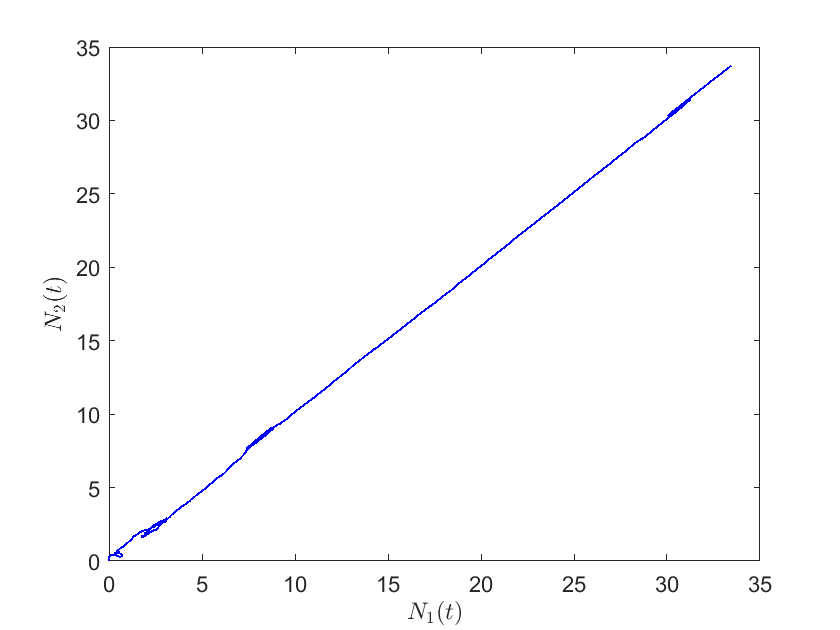
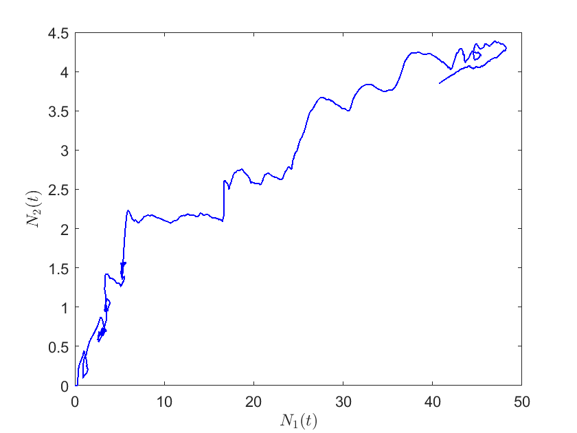
In case λ^0|ρ2(μ^2μ^1)+λ^1λ^2|subscript^𝜆0superscript𝜌2subscript^𝜇2subscript^𝜇1subscript^𝜆1subscript^𝜆2\widehat{\lambda}_{0}\leq|\rho^{2}(\widehat{\mu}_{2}-\widehat{\mu}_{1})+\widehat{\lambda}_{1}-\widehat{\lambda}_{2}|, i.e., the weakly pooled case, there is a spectrum of possible drift directions, depending on how large is the proportion of the dedicated traffic. Moreover, the approximated joint orbit queue length distribution cannot any more written in such an elegant form and is not well defined. An illustration of both scenarios are given in Figure 9, where we performed some simulations. Note that in the strongly pooled case, orbit queue lengths grow in tandem as expected; Figure 9 (left). In Figure 9 (right), λ^0<|ρ2(μ^2μ^1)+λ^1λ^2|subscript^𝜆0superscript𝜌2subscript^𝜇2subscript^𝜇1subscript^𝜆1subscript^𝜆2\widehat{\lambda}_{0}<|\rho^{2}(\widehat{\mu}_{2}-\widehat{\mu}_{1})+\widehat{\lambda}_{1}-\widehat{\lambda}_{2}|, and λ1>λ0>λ2subscript𝜆1subscript𝜆0subscript𝜆2\lambda_{1}>\lambda_{0}>\lambda_{2}, α1>α2subscript𝛼1subscript𝛼2\alpha_{1}>\alpha_{2}, we observe that N2(t)subscript𝑁2𝑡N_{2}(t) lags behind N1(t)subscript𝑁1𝑡N_{1}(t).

Refer to caption
Refer to caption
Figure 9: Orbit dynamics when ρ<1𝜌1\rho<1, α1>α2subscript𝛼1subscript𝛼2\alpha_{1}>\alpha_{2}, and λ^0>|ρ2(μ^2μ^1)+λ^1λ^2|subscript^𝜆0superscript𝜌2subscript^𝜇2subscript^𝜇1subscript^𝜆1subscript^𝜆2\widehat{\lambda}_{0}>|\rho^{2}(\widehat{\mu}_{2}-\widehat{\mu}_{1})+\widehat{\lambda}_{1}-\widehat{\lambda}_{2}| (left), and when λ^0<|ρ2(μ^2μ^1)+λ^1λ^2|subscript^𝜆0superscript𝜌2subscript^𝜇2subscript^𝜇1subscript^𝜆1subscript^𝜆2\widehat{\lambda}_{0}<|\rho^{2}(\widehat{\mu}_{2}-\widehat{\mu}_{1})+\widehat{\lambda}_{1}-\widehat{\lambda}_{2}|, and λ1>λ0>λ2subscript𝜆1subscript𝜆0subscript𝜆2\lambda_{1}>\lambda_{0}>\lambda_{2} (right).

5 Proofs of main results

To improve the readability of the paper we group in this section the proofs of the main results presented in section 4.

5.1 Proof of Theorem 4.1

The proof follows the lines in [26], and a series of results are needed to be proven. Note that {Y(n);n0}𝑌𝑛𝑛0\{Y(n);n\geq 0\} is a discrete time QBD process with the following block structured transition matrix

PY=(L0A1A1A0A1A1A0A1A1A0A1),subscript𝑃𝑌matrixsubscript𝐿0subscript𝐴1missing-subexpressionmissing-subexpressionmissing-subexpressionsubscript𝐴1subscript𝐴0subscript𝐴1missing-subexpressionmissing-subexpressionmissing-subexpressionsubscript𝐴1subscript𝐴0subscript𝐴1missing-subexpressionmissing-subexpressionmissing-subexpressionsubscript𝐴1subscript𝐴0subscript𝐴1missing-subexpressionmissing-subexpressionmissing-subexpressionP_{Y}=\begin{pmatrix}L_{0}&A_{1}&&&\\ A_{-1}&A_{0}&A_{1}&&\\ &A_{-1}&A_{0}&A_{1}&\\ &&A_{-1}&A_{0}&A_{1}\\ &&&\ddots&\ddots&\ddots\end{pmatrix},

where the infinite dimensional matrices L𝐿L, Aisubscript𝐴𝑖A_{i}, i=0,±1𝑖0plus-or-minus1i=0,\pm 1 are

(L)l,l=(Y(n+1)=(0,l,1)|Y(n)=(0,l,1)),l,l,(Ai)l,l=(Y(n+1)=(m+i,l,1)|Y(n)=(m,l,1)),l,l,m1,subscript𝐿𝑙superscript𝑙absent𝑌𝑛1conditional0superscript𝑙1𝑌𝑛0𝑙1𝑙superscript𝑙subscriptsubscript𝐴𝑖𝑙superscript𝑙absentformulae-sequence𝑌𝑛1conditional𝑚𝑖superscript𝑙1𝑌𝑛𝑚𝑙1𝑙superscript𝑙𝑚1\begin{array}[]{rl}(L)_{l,l^{\prime}}=&\mathbb{P}(Y(n+1)=(0,l^{\prime},1)|Y(n)=(0,l,1)),\,l,l^{\prime}\in\mathbb{Z},\\ (A_{i})_{l,l^{\prime}}=&\mathbb{P}(Y(n+1)=(m+i,l^{\prime},1)|Y(n)=(m,l,1)),\,l,l^{\prime}\in\mathbb{Z},\,m\geq 1,\end{array}

with their elements (i.e., the one step transition probabilities) are given in (4.1). Under the stability condition, the stationary distribution exists. Denote it by the row vector 𝝅=(𝝅𝟎,𝝅𝟏,)𝝅subscript𝝅0subscript𝝅1\boldsymbol{\pi}=(\boldsymbol{\pi_{0}},\boldsymbol{\pi_{1}},\ldots). It is well known that the stationary distribution has the following matrix geometric form:

𝝅𝒎=𝝅𝟎Rm,m1,formulae-sequencesubscript𝝅𝒎subscript𝝅0superscript𝑅𝑚𝑚1\boldsymbol{\pi_{m}}=\boldsymbol{\pi_{0}}R^{m},\,m\geq 1, (5.1)

where R𝑅R is the minimal nonnegative solution of the equation

R=A1+RA0+R2A1.𝑅subscript𝐴1𝑅subscript𝐴0superscript𝑅2subscript𝐴1R=A_{1}+RA_{0}+R^{2}A_{-1}.

Since the size of R𝑅R is infinite, conditions for geometric tail decay rate of (5.1) are given in [26]:

Proposition 1.

(Theorem 2.1 in [26]) Let AA1+A0+A1𝐴subscript𝐴1subscript𝐴0subscript𝐴1A\equiv A_{-1}+A_{0}+A_{1} is irreducible and aperiodic, and assume that the Markov additive process generated by {Ai,i=0,±1}formulae-sequencesubscript𝐴𝑖𝑖0plus-or-minus1\{A_{i},i=0,\pm 1\} is 1-arithmetic. If there exists z>1𝑧1z>1 and positive vectors 𝐱𝐱\mathbf{x}, 𝐲𝐲\mathbf{y} such that

𝐱=𝐱A(z),𝐲=A(z)𝐲,formulae-sequence𝐱𝐱subscript𝐴𝑧𝐲subscript𝐴𝑧𝐲\displaystyle\mathbf{x}=\mathbf{x}A_{*}(z),\,\mathbf{y}=A_{*}(z)\mathbf{y}, (5.2)
𝐱𝐲<,𝐱𝐲\displaystyle\mathbf{x}\mathbf{y}<\infty, (5.3)

where A(w)=w1A1+A0+wA1subscript𝐴𝑤superscript𝑤1subscript𝐴1subscript𝐴0𝑤subscript𝐴1A_{*}(w)=w^{-1}A_{-1}+A_{0}+wA_{1}, w0𝑤0w\neq 0. Then R𝑅R has left and right eigenvectors 𝐱𝐱\mathbf{x} and 𝐫(IA0RA1z1A1)𝐲𝐫𝐼subscript𝐴0𝑅subscript𝐴1superscript𝑧1subscript𝐴1𝐲\mathbf{r}\equiv(I-A_{0}-RA_{-1}-z^{-1}A_{-1})\mathbf{y}, respectively, with eigenvalue z1superscript𝑧1z^{-1}. Moreover, if

𝝅0𝐲<,subscript𝝅0𝐲\boldsymbol{\pi}_{0}\mathbf{y}<\infty, (5.4)

then

limmzn𝝅m=𝝅0𝐫𝐱𝐫𝐱.subscript𝑚superscript𝑧𝑛subscript𝝅𝑚subscript𝝅0𝐫𝐱𝐫𝐱\displaystyle\lim_{m\to\infty}z^{n}\boldsymbol{\pi}_{m}=\frac{\boldsymbol{\pi}_{0}\mathbf{r}}{\mathbf{x}\mathbf{r}}\mathbf{x}. (5.5)
Remark 6.

It is easy to see that for our queueing model both the aperiodicity and the irreducibility of A𝐴A are easily verified. Moreover,the 1-arithmetic property of the Markov additive process generated by {Ai;i=0,±1}formulae-sequencesubscript𝐴𝑖𝑖0plus-or-minus1\{A_{i};i=0,\pm 1\} is readily satisfied by its transition structure.

For our case the matrix A(z)subscript𝐴𝑧A_{*}(z) is given by

A(z)=3210123( ) 2a1a0a11a1a0a10c1c0c11b1b0b12b1b0b1,A_{*}(z)=\bordermatrix{\text{}&\ldots&-3&-2&-1&0&1&2&3&\ldots\cr\vdots&\ddots&\ddots&\ddots&&&&&&\cr-2&&a_{-1}&a_{0}&a_{1}&&&&&\cr-1&&&a_{-1}&a_{0}&a_{1}&&&&\cr 0&&&&c_{-1}&c_{0}&c_{1}&&&\cr 1&&&&&b_{-1}&b_{0}&b_{1}&&\cr 2&&&&&&b_{-1}&b_{0}&b_{1}&\cr\vdots&&&&&&&\ddots&\ddots&\ddots},

where

a1=μ^2λ+α1+α2z1+λ1,a0=α1+α2+λμλ+α1+α2,a1=μ^1λ+α1+α2+(λ0+λ2)z,c1=μ^2λ+α1+α2z1+λ1+λ02,c0=a0,c1=μ^1λ+α1+α2z1+λ02+λ2,b1=μ^2λ+α1+α2+(λ0+λ1)z,b0=a0,b1=μ^1λ+α1+α2z1+λ2.formulae-sequencesubscript𝑎1subscript^𝜇2𝜆subscript𝛼1subscript𝛼2superscript𝑧1subscript𝜆1formulae-sequencesubscript𝑎0subscript𝛼1subscript𝛼2𝜆𝜇𝜆subscript𝛼1subscript𝛼2subscript𝑎1subscript^𝜇1𝜆subscript𝛼1subscript𝛼2subscript𝜆0subscript𝜆2𝑧formulae-sequencesubscript𝑐1subscript^𝜇2𝜆subscript𝛼1subscript𝛼2superscript𝑧1subscript𝜆1subscript𝜆02formulae-sequencesubscript𝑐0subscript𝑎0subscript𝑐1subscript^𝜇1𝜆subscript𝛼1subscript𝛼2superscript𝑧1subscript𝜆02subscript𝜆2formulae-sequencesubscript𝑏1subscript^𝜇2𝜆subscript𝛼1subscript𝛼2subscript𝜆0subscript𝜆1𝑧formulae-sequencesubscript𝑏0subscript𝑎0subscript𝑏1subscript^𝜇1𝜆subscript𝛼1subscript𝛼2superscript𝑧1subscript𝜆2\begin{array}[]{c}a_{-1}=\frac{\widehat{\mu}_{2}}{\lambda+\alpha_{1}+\alpha_{2}}z^{-1}+\lambda_{1},\,a_{0}=\alpha_{1}+\alpha_{2}+\frac{\lambda\mu}{\lambda+\alpha_{1}+\alpha_{2}},\,a_{1}=\frac{\widehat{\mu}_{1}}{\lambda+\alpha_{1}+\alpha_{2}}+(\lambda_{0}+\lambda_{2})z,\\ c_{-1}=\frac{\widehat{\mu}_{2}}{\lambda+\alpha_{1}+\alpha_{2}}z^{-1}+\lambda_{1}+\frac{\lambda_{0}}{2},\,c_{0}=a_{0},\,c_{1}=\frac{\widehat{\mu}_{1}}{\lambda+\alpha_{1}+\alpha_{2}}z^{-1}+\frac{\lambda_{0}}{2}+\lambda_{2},\\ b_{-1}=\frac{\widehat{\mu}_{2}}{\lambda+\alpha_{1}+\alpha_{2}}+(\lambda_{0}+\lambda_{1})z,\,b_{0}=a_{0},\,b_{1}=\frac{\widehat{\mu}_{1}}{\lambda+\alpha_{1}+\alpha_{2}}z^{-1}+\lambda_{2}.\end{array}

Denote the left and the right invariant vectors of A(z)subscript𝐴𝑧A_{*}(z), z>1𝑧1z>1 by

𝐱(z)=(,x1(z),x0,x1(z),),𝐲(z)=(,y1(z),y0,y1(z),)T.formulae-sequence𝐱𝑧subscript𝑥1𝑧subscript𝑥0subscript𝑥1𝑧𝐲𝑧superscriptsubscript𝑦1𝑧subscript𝑦0subscript𝑦1𝑧𝑇\begin{array}[]{c}\mathbf{x}(z)=(\ldots,x_{-1}(z),x_{0},x_{1}(z),\ldots),\,\mathbf{y}(z)=(\ldots,y_{-1}(z),y_{0},y_{1}(z),\ldots)^{T}.\end{array}

We are left to examine conditions (5.2), (5.3), (5.4). To this end, let

βi,j(z)=(λ^+μ^1+μ^2)24(μ^i+(λ^0+λ^j)z)(μ^jz1+λ^i),i,j=1,2,f(z)=μ^2z1+λ^1+λ^022(μ^2z1+λ^1)(1β1,2(z)λ^+μ^1+μ^2)+μ^1z1+λ^2+λ^022(μ^1z1+λ^2)(1β2,1(z)λ^+μ^1+μ^2).subscript𝛽𝑖𝑗𝑧absentformulae-sequencesuperscript^𝜆subscript^𝜇1subscript^𝜇224subscript^𝜇𝑖subscript^𝜆0subscript^𝜆𝑗𝑧subscript^𝜇𝑗superscript𝑧1subscript^𝜆𝑖𝑖𝑗12𝑓𝑧absentsubscript^𝜇2superscript𝑧1subscript^𝜆1subscript^𝜆022subscript^𝜇2superscript𝑧1subscript^𝜆11subscript𝛽12𝑧^𝜆subscript^𝜇1subscript^𝜇2subscript^𝜇1superscript𝑧1subscript^𝜆2subscript^𝜆022subscript^𝜇1superscript𝑧1subscript^𝜆21subscript𝛽21𝑧^𝜆subscript^𝜇1subscript^𝜇2\begin{array}[]{rl}\beta_{i,j}(z)=&(\widehat{\lambda}+\widehat{\mu}_{1}+\widehat{\mu}_{2})^{2}-4(\widehat{\mu}_{i}+(\widehat{\lambda}_{0}+\widehat{\lambda}_{j})z)(\widehat{\mu}_{j}z^{-1}+\widehat{\lambda}_{i}),\,i,j=1,2,\\ f(z)=&\frac{\widehat{\mu}_{2}z^{-1}+\widehat{\lambda}_{1}+\frac{\widehat{\lambda}_{0}}{2}}{2(\widehat{\mu}_{2}z^{-1}+\widehat{\lambda}_{1})}(1-\frac{\sqrt{\beta_{1,2}(z)}}{\widehat{\lambda}+\widehat{\mu}_{1}+\widehat{\mu}_{2}})+\frac{\widehat{\mu}_{1}z^{-1}+\widehat{\lambda}_{2}+\frac{\widehat{\lambda}_{0}}{2}}{2(\widehat{\mu}_{1}z^{-1}+\widehat{\lambda}_{2})}(1-\frac{\sqrt{\beta_{2,1}(z)}}{\widehat{\lambda}+\widehat{\mu}_{1}+\widehat{\mu}_{2}}).\end{array}
Lemma 4.

For the censored chain {Y(n);n0}𝑌𝑛𝑛0\{Y(n);n\geq 0\} on the busy states of our GJSOQ, the conditions (5.2), (5.3) hold if and only if there exists a z>1𝑧1z>1 such that

β1,2(z)>0,β2,1(z)>0,formulae-sequencesubscript𝛽12𝑧0subscript𝛽21𝑧0\displaystyle\beta_{1,2}(z)>0,\,\beta_{2,1}(z)>0, (5.6)

and f(z)=1𝑓𝑧1f(z)=1. In such a case, the left and right invariant vectors 𝐱(z)𝐱𝑧\mathbf{x}(z) and 𝐲(z)𝐲𝑧\mathbf{y}(z) of A(z)subscript𝐴𝑧A_{*}(z) satisfying 𝐱(z)𝐲(z)<𝐱𝑧𝐲𝑧\mathbf{x}(z)\mathbf{y}(z)<\infty have the following forms:

xl(z)={(1+λ^02(μ^2z1+λ^1))x0ηmin|l|,l1,(1+λ^02(μ^1z1+λ^2))x0θminl,l1,,yl(z)={y0ηmax|l|,l1,y0θmaxl,l1,subscript𝑥𝑙𝑧cases1subscript^𝜆02subscript^𝜇2superscript𝑧1subscript^𝜆1subscript𝑥0superscriptsubscript𝜂𝑚𝑖𝑛𝑙𝑙11subscript^𝜆02subscript^𝜇1superscript𝑧1subscript^𝜆2subscript𝑥0superscriptsubscript𝜃𝑚𝑖𝑛𝑙𝑙1subscript𝑦𝑙𝑧casessubscript𝑦0superscriptsubscript𝜂𝑚𝑎𝑥𝑙𝑙1subscript𝑦0superscriptsubscript𝜃𝑚𝑎𝑥𝑙𝑙1\begin{array}[]{rl}x_{l}(z)=\left\{\begin{array}[]{ll}(1+\frac{\widehat{\lambda}_{0}}{2(\widehat{\mu}_{2}z^{-1}+\widehat{\lambda}_{1})})x_{0}\eta_{min}^{|l|},&l\leq-1,\\ (1+\frac{\widehat{\lambda}_{0}}{2(\widehat{\mu}_{1}z^{-1}+\widehat{\lambda}_{2})})x_{0}\theta_{min}^{l},&l\geq 1,\end{array}\right.,&y_{l}(z)=\left\{\begin{array}[]{ll}y_{0}\eta_{max}^{-|l|},&l\leq-1,\\ y_{0}\theta_{max}^{-l},&l\geq 1,\end{array}\right.\end{array} (5.7)

where ηmin<ηmaxsubscript𝜂𝑚𝑖𝑛subscript𝜂𝑚𝑎𝑥\eta_{min}<\eta_{max} are the roots of the equation:

ϕ(η):=η2(μ^1+(λ^0+λ^2)z)η(λ^+μ^1+μ^2)+μ^2z1+λ^1=0,assignsubscriptitalic-ϕ𝜂superscript𝜂2subscript^𝜇1subscript^𝜆0subscript^𝜆2𝑧𝜂^𝜆subscript^𝜇1subscript^𝜇2subscript^𝜇2superscript𝑧1subscript^𝜆10\displaystyle\phi_{-}(\eta):=\eta^{2}(\widehat{\mu}_{1}+(\widehat{\lambda}_{0}+\widehat{\lambda}_{2})z)-\eta(\widehat{\lambda}+\widehat{\mu}_{1}+\widehat{\mu}_{2})+\widehat{\mu}_{2}z^{-1}+\widehat{\lambda}_{1}=0, (5.8)

and θmin<θmaxsubscript𝜃𝑚𝑖𝑛subscript𝜃𝑚𝑎𝑥\theta_{min}<\theta_{max} are the roots of the equation:

ϕ+(θ):=θ2(μ^2+(λ^0+λ^1)z)θ(λ^+μ^1+μ^2)+μ^1z1+λ^2=0.assignsubscriptitalic-ϕ𝜃superscript𝜃2subscript^𝜇2subscript^𝜆0subscript^𝜆1𝑧𝜃^𝜆subscript^𝜇1subscript^𝜇2subscript^𝜇1superscript𝑧1subscript^𝜆20\displaystyle\phi_{+}(\theta):=\theta^{2}(\widehat{\mu}_{2}+(\widehat{\lambda}_{0}+\widehat{\lambda}_{1})z)-\theta(\widehat{\lambda}+\widehat{\mu}_{1}+\widehat{\mu}_{2})+\widehat{\mu}_{1}z^{-1}+\widehat{\lambda}_{2}=0. (5.9)
Proof.

See Appendix C.∎

Remark 7.

Note that from (5.8), (5.9),

ηmin=λ^+μ^1+μ^2β1,2(z)2(μ^1+(λ^2+λ^0)z),ηmax=λ^+μ^1+μ^2+β1,2(z)2(μ^1+(λ^2+λ^0)z),θmin=λ^+μ^1+μ^2β2,1(z)2(μ^2+(λ^1+λ^0)z),θmax=λ^+μ^1+μ^2+β2,1(z)2(μ^2+(λ^1+λ^0)z).subscript𝜂𝑚𝑖𝑛absent^𝜆subscript^𝜇1subscript^𝜇2subscript𝛽12𝑧2subscript^𝜇1subscript^𝜆2subscript^𝜆0𝑧subscript𝜂𝑚𝑎𝑥absent^𝜆subscript^𝜇1subscript^𝜇2subscript𝛽12𝑧2subscript^𝜇1subscript^𝜆2subscript^𝜆0𝑧missing-subexpressionsubscript𝜃𝑚𝑖𝑛absent^𝜆subscript^𝜇1subscript^𝜇2subscript𝛽21𝑧2subscript^𝜇2subscript^𝜆1subscript^𝜆0𝑧subscript𝜃𝑚𝑎𝑥absent^𝜆subscript^𝜇1subscript^𝜇2subscript𝛽21𝑧2subscript^𝜇2subscript^𝜆1subscript^𝜆0𝑧missing-subexpression\begin{array}[]{llcrl}\eta_{min}=&\frac{\widehat{\lambda}+\widehat{\mu}_{1}+\widehat{\mu}_{2}-\sqrt{\beta_{1,2}(z)}}{2(\widehat{\mu}_{1}+(\widehat{\lambda}_{2}+\widehat{\lambda}_{0})z)},&\eta_{max}=&\frac{\widehat{\lambda}+\widehat{\mu}_{1}+\widehat{\mu}_{2}+\sqrt{\beta_{1,2}(z)}}{2(\widehat{\mu}_{1}+(\widehat{\lambda}_{2}+\widehat{\lambda}_{0})z)},\\ \theta_{min}=&\frac{\widehat{\lambda}+\widehat{\mu}_{1}+\widehat{\mu}_{2}-\sqrt{\beta_{2,1}(z)}}{2(\widehat{\mu}_{2}+(\widehat{\lambda}_{1}+\widehat{\lambda}_{0})z)},&\theta_{max}=&\frac{\widehat{\lambda}+\widehat{\mu}_{1}+\widehat{\mu}_{2}+\sqrt{\beta_{2,1}(z)}}{2(\widehat{\mu}_{2}+(\widehat{\lambda}_{1}+\widehat{\lambda}_{0})z)}.\end{array}

We now turn our attention in the solution of the equation f(z)=1𝑓𝑧1f(z)=1. To improve the readability, set γ1=μ^1ρ2+λ^2subscript𝛾1subscript^𝜇1superscript𝜌2subscript^𝜆2\gamma_{1}=\widehat{\mu}_{1}\rho^{2}+\widehat{\lambda}_{2}, γ2=μ^2ρ2+λ^1subscript𝛾2subscript^𝜇2superscript𝜌2subscript^𝜆1\gamma_{2}=\widehat{\mu}_{2}\rho^{2}+\widehat{\lambda}_{1}. Note that γ1+γ2+λ^0=ρ(λ^+μ^1+μ^2)subscript𝛾1subscript𝛾2subscript^𝜆0𝜌^𝜆subscript^𝜇1subscript^𝜇2\gamma_{1}+\gamma_{2}+\widehat{\lambda}_{0}=\rho(\widehat{\lambda}+\widehat{\mu}_{1}+\widehat{\mu}_{2}).

Lemma 5.

z=ρ2𝑧superscript𝜌2z=\rho^{-2} is the only solution of f(z)=1𝑓𝑧1f(z)=1, z>1𝑧1z>1, and

(ηmin,ηmax)=(ργ2γ1+λ^0,ρ) or (ρ,ργ2γ1+λ^0),subscript𝜂𝑚𝑖𝑛subscript𝜂𝑚𝑎𝑥𝜌subscript𝛾2subscript𝛾1subscript^𝜆0𝜌 or 𝜌𝜌subscript𝛾2subscript𝛾1subscript^𝜆0\displaystyle(\eta_{min},\eta_{max})=(\rho\frac{\gamma_{2}}{\gamma_{1}+\widehat{\lambda}_{0}},\rho)\text{ or }(\rho,\rho\frac{\gamma_{2}}{\gamma_{1}+\widehat{\lambda}_{0}}), (5.10)
(θmin,θmax)=(ργ1γ2+λ^0,ρ) or (ρ,ργ1γ2+λ^0).subscript𝜃𝑚𝑖𝑛subscript𝜃𝑚𝑎𝑥𝜌subscript𝛾1subscript𝛾2subscript^𝜆0𝜌 or 𝜌𝜌subscript𝛾1subscript𝛾2subscript^𝜆0\displaystyle(\theta_{min},\theta_{max})=(\rho\frac{\gamma_{1}}{\gamma_{2}+\widehat{\lambda}_{0}},\rho)\text{ or }(\rho,\rho\frac{\gamma_{1}}{\gamma_{2}+\widehat{\lambda}_{0}}). (5.11)
Proof.

See Appendix D. ∎

The results given in Lemmas 4, 5 provide the basic ingredients for the proof of Theorem 4.1. Note that based on Lemma 5 there are four cases for the expression of 𝐱(ρ2)𝐱superscript𝜌2\mathbf{x}(\rho^{-2}) based on the possible values of ηminsubscript𝜂𝑚𝑖𝑛\eta_{min}, θminsubscript𝜃𝑚𝑖𝑛\theta_{min}. In particular,

(ηminθmin)=(ργ2γ1+λ^0ργ1γ2+λ^0) or (ρργ1γ2+λ^0) or (ργ2γ1+λ^0ρ) or (ρρ).matrixsubscript𝜂𝑚𝑖𝑛subscript𝜃𝑚𝑖𝑛absentmatrix𝜌subscript𝛾2subscript𝛾1subscript^𝜆0𝜌subscript𝛾1subscript𝛾2subscript^𝜆0 or matrix𝜌𝜌subscript𝛾1subscript𝛾2subscript^𝜆0 or matrix𝜌subscript𝛾2subscript𝛾1subscript^𝜆0𝜌 or matrix𝜌𝜌\begin{array}[]{rl}\begin{pmatrix}\eta_{min}\\ \theta_{min}\end{pmatrix}=&\begin{pmatrix}\rho\frac{\gamma_{2}}{\gamma_{1}+\widehat{\lambda}_{0}}\\ \rho\frac{\gamma_{1}}{\gamma_{2}+\widehat{\lambda}_{0}}\end{pmatrix}\text{ or }\begin{pmatrix}\rho\\ \rho\frac{\gamma_{1}}{\gamma_{2}+\widehat{\lambda}_{0}}\end{pmatrix}\text{ or }\begin{pmatrix}\rho\frac{\gamma_{2}}{\gamma_{1}+\widehat{\lambda}_{0}}\\ \rho\end{pmatrix}\text{ or }\begin{pmatrix}\rho\\ \rho\end{pmatrix}.\end{array}

The last one is rejected since corresponds to the case γ1+λ^0γ2subscript𝛾1subscript^𝜆0subscript𝛾2\gamma_{1}+\widehat{\lambda}_{0}\leq\gamma_{2}, γ2+λ^0γ1subscript𝛾2subscript^𝜆0subscript𝛾1\gamma_{2}+\widehat{\lambda}_{0}\leq\gamma_{1}, which is impossible since λ0>0subscript𝜆00\lambda_{0}>0. It is easily seen that only the first pair satisfies 𝐱(ρ2)=𝐱(ρ2)A(ρ2)𝐱superscript𝜌2𝐱superscript𝜌2subscript𝐴superscript𝜌2\mathbf{x}(\rho^{-2})=\mathbf{x}(\rho^{-2})A_{*}(\rho^{-2}), which means that A(ρ2)subscript𝐴superscript𝜌2A_{*}(\rho^{-2}) is 1-positive. Note that in such a case ργ2γ1+λ^0<ργ2γ1<λ^0𝜌subscript𝛾2subscript𝛾1subscript^𝜆0𝜌subscript𝛾2subscript𝛾1subscript^𝜆0\rho\frac{\gamma_{2}}{\gamma_{1}+\widehat{\lambda}_{0}}<\rho\Rightarrow\gamma_{2}-\gamma_{1}<\widehat{\lambda}_{0}, and ργ1γ2+λ^0<ργ1γ2<λ^0𝜌subscript𝛾1subscript𝛾2subscript^𝜆0𝜌subscript𝛾1subscript𝛾2subscript^𝜆0\rho\frac{\gamma_{1}}{\gamma_{2}+\widehat{\lambda}_{0}}<\rho\Rightarrow\gamma_{1}-\gamma_{2}<\widehat{\lambda}_{0}, which is equivalent to |γ1γ2|<λ^0subscript𝛾1subscript𝛾2subscript^𝜆0|\gamma_{1}-\gamma_{2}|<\widehat{\lambda}_{0} or to |λ^2λ^1+ρ2(μ1μ2)|<λ^0subscript^𝜆2subscript^𝜆1superscript𝜌2subscript𝜇1subscript𝜇2subscript^𝜆0|\widehat{\lambda}_{2}-\widehat{\lambda}_{1}+\rho^{2}(\mu_{1}-\mu_{2})|<\widehat{\lambda}_{0} (note that this case is equivalent to the so called strongly pooled case in [15]).

Now it remains to verify the boundary condition (5.4). From Lemma 5 we know that ηmax=θmax=ρsubscript𝜂𝑚𝑎𝑥subscript𝜃𝑚𝑎𝑥𝜌\eta_{max}=\theta_{max}=\rho. Thus, 𝝅0𝐲<subscript𝝅0𝐲\boldsymbol{\pi}_{0}\mathbf{y}<\infty implies

l=0ρl((N1=l,N2=0,C=1)+(N1=0,N2=l,C=1))<,superscriptsubscript𝑙0superscript𝜌𝑙formulae-sequencesubscript𝑁1𝑙formulae-sequencesubscript𝑁20𝐶1formulae-sequencesubscript𝑁10formulae-sequencesubscript𝑁2𝑙𝐶1\sum_{l=0}^{\infty}\rho^{-l}(\mathbb{P}(N_{1}=l,N_{2}=0,C=1)+\mathbb{P}(N_{1}=0,N_{2}=l,C=1))<\infty,

where {(N1,N2,C)}subscript𝑁1subscript𝑁2𝐶\{(N_{1},N_{2},C)\} is the stationary version of {X(n);n0}𝑋𝑛𝑛0\{X(n);n\geq 0\}. The last inequality is the same as condition C.10 in [15], which was proved under the corresponding conditions max{ρ1,ρ2}<ρ<1𝑚𝑎𝑥subscript𝜌1subscript𝜌2𝜌1max\{\rho_{1},\rho_{2}\}<\rho<1, and |λ^2λ^1+ρ2(μ1μ2)|<λ^0subscript^𝜆2subscript^𝜆1superscript𝜌2subscript𝜇1subscript𝜇2subscript^𝜆0|\widehat{\lambda}_{2}-\widehat{\lambda}_{1}+\rho^{2}(\mu_{1}-\mu_{2})|<\widehat{\lambda}_{0} in [15, Proposition 1], following [28, Theorem 14.3.7], so further details are omitted.

Following [26, Definition 2.2], the two orbit queue are strongly balanced, if the difference between orbit queue lengths (i.e., the background process) is dominated by the level process, i.e., min{N1,n,N2,n}𝑚𝑖𝑛subscript𝑁1𝑛subscript𝑁2𝑛min\{N_{1,n},N_{2,n}\}. Intuitively, it means that the level process has more influence when the same scaling is applied to the level and background process. This is equivalent with the condition

liml+ρ2lxl(ρ2)=limlρ2lxl(ρ2)=0.subscript𝑙superscript𝜌2𝑙subscript𝑥𝑙superscript𝜌2subscript𝑙superscript𝜌2𝑙subscript𝑥𝑙superscript𝜌20\lim_{l\to+\infty}\rho^{-2l}x_{l}(\rho^{-2})=\lim_{l\to-\infty}\rho^{2l}x_{l}(\rho^{-2})=0.

Noting (4.3), it is easily realized that this is the case if and only if γ2<ρ(γ1+λ^0)subscript𝛾2𝜌subscript𝛾1subscript^𝜆0\gamma_{2}<\rho(\gamma_{1}+\widehat{\lambda}_{0}), γ1<ρ(γ2+λ^0)subscript𝛾1𝜌subscript𝛾2subscript^𝜆0\gamma_{1}<\rho(\gamma_{2}+\widehat{\lambda}_{0}).

5.2 Proof of Lemma 2

Starting with region I (i1much-greater-than𝑖1i\gg 1, j1much-greater-than𝑗1j\gg 1), equations (2.1), (2.2) are the only relevant. By introducing the new variables m=i+j𝑚𝑖𝑗m=i+j, n=ji𝑛𝑗𝑖n=j-i, and setting pi,j(k)Rm,n(k)subscript𝑝𝑖𝑗𝑘subscript𝑅𝑚𝑛𝑘p_{i,j}(k)\equiv R_{m,n}(k), (2.1), (2.2) become

Rm,n(0)=μλ+2αRm,n(1),subscript𝑅𝑚𝑛0𝜇𝜆2𝛼subscript𝑅𝑚𝑛1\displaystyle R_{m,n}(0)=\frac{\mu}{\lambda+2\alpha}R_{m,n}(1), (5.12)
(λ+2α)Rm,n(1)=[λ0H(1n)+λ+]Rm1,n1(1)𝜆2𝛼subscript𝑅𝑚𝑛1delimited-[]subscript𝜆0𝐻1𝑛subscript𝜆subscript𝑅𝑚1𝑛11\displaystyle(\lambda+2\alpha)R_{m,n}(1)=[\lambda_{0}H(1-n)+\lambda_{+}]R_{m-1,n-1}(1)
+[λ0H(n+1)+λ+]Rm1,n+1(1)+λRm,n(0)+α[Rm+1,n1(0)+Rm+1,n+1(0)],delimited-[]subscript𝜆0𝐻𝑛1subscript𝜆subscript𝑅𝑚1𝑛11𝜆subscript𝑅𝑚𝑛0𝛼delimited-[]subscript𝑅𝑚1𝑛10subscript𝑅𝑚1𝑛10\displaystyle+[\lambda_{0}H(n+1)+\lambda_{+}]R_{m-1,n+1}(1)+\lambda R_{m,n}(0)+\alpha[R_{m+1,n-1}(0)+R_{m+1,n+1}(0)], (5.13)

Substitute (5.12) to (5.13) yields

(λ^+2μ^)Rm,n(1)=[λ^0H(1n)+λ^+]Rm1,n1(1)^𝜆2^𝜇subscript𝑅𝑚𝑛1delimited-[]subscript^𝜆0𝐻1𝑛subscript^𝜆subscript𝑅𝑚1𝑛11\displaystyle(\widehat{\lambda}+2\widehat{\mu})R_{m,n}(1)=[\widehat{\lambda}_{0}H(1-n)+\widehat{\lambda}_{+}]R_{m-1,n-1}(1)
+[λ^0H(n+1)+λ^+]Rm1,n+1(1)+μ^[Rm+1,n1(1)+Rm,n(1)],delimited-[]subscript^𝜆0𝐻𝑛1subscript^𝜆subscript𝑅𝑚1𝑛11^𝜇delimited-[]subscript𝑅𝑚1𝑛11subscript𝑅𝑚𝑛1\displaystyle+[\widehat{\lambda}_{0}H(n+1)+\widehat{\lambda}_{+}]R_{m-1,n+1}(1)+\widehat{\mu}[R_{m+1,n-1}(1)+R_{m,n}(1)], (5.14)

where λ^=λ(λ+2α)^𝜆𝜆𝜆2𝛼\widehat{\lambda}=\lambda(\lambda+2\alpha), λ=λ0+2λ+𝜆subscript𝜆02subscript𝜆\lambda=\lambda_{0}+2\lambda_{+}, λ^l=λl(λ+2α)subscript^𝜆𝑙subscript𝜆𝑙𝜆2𝛼\widehat{\lambda}_{l}=\lambda_{l}(\lambda+2\alpha), l=0,+𝑙0l=0,+, μ^=αμ^𝜇𝛼𝜇\widehat{\mu}=\alpha\mu. Note that regarding variable m𝑚m, (5.14) is second-order difference equation with constant coefficients, which admits solutions of the form R(m,n,1)=γmQ(n)𝑅𝑚𝑛1superscript𝛾𝑚𝑄𝑛R(m,n,1)=\gamma^{m}Q(n), where γ𝛾\gamma a constant to be determined. Substituting in (5.14) we realize that Q(n)𝑄𝑛Q(n) satisfies

(λ^+2μ^)Q(n)=[λ^0H(1n)+λ^+γ+μ^γ]Q(n1)+[λ^0H(1+n)+λ^+γ+μ^γ]Q(n+1).^𝜆2^𝜇𝑄𝑛absentdelimited-[]subscript^𝜆0𝐻1𝑛subscript^𝜆𝛾^𝜇𝛾𝑄𝑛1delimited-[]subscript^𝜆0𝐻1𝑛subscript^𝜆𝛾^𝜇𝛾𝑄𝑛1\begin{array}[]{rl}(\widehat{\lambda}+2\widehat{\mu})Q(n)=&[\frac{\widehat{\lambda}_{0}H(1-n)+\widehat{\lambda}_{+}}{\gamma}+\widehat{\mu}\gamma]Q(n-1)+[\frac{\widehat{\lambda}_{0}H(1+n)+\widehat{\lambda}_{+}}{\gamma}+\widehat{\mu}\gamma]Q(n+1).\end{array} (5.15)

Note that symmetry implies that Q(n)=Q(n)𝑄𝑛𝑄𝑛Q(n)=Q(-n), and thus, it is sufficient to only consider n0𝑛0n\geq 0. Then, for n=0𝑛0n=0, (5.14) gives

(λ^+2μ^)Q(0)=2[λ^0+λ^+γ+μ^γ]Q(1).^𝜆2^𝜇𝑄02delimited-[]subscript^𝜆0subscript^𝜆𝛾^𝜇𝛾𝑄1(\widehat{\lambda}+2\widehat{\mu})Q(0)=2[\frac{\widehat{\lambda}_{0}+\widehat{\lambda}_{+}}{\gamma}+\widehat{\mu}\gamma]Q(1). (5.16)

Setting n=1𝑛1n=1 in (5.15), and using (5.16) we obtain,

[λ^0+λ^+γ+μ^γ]Q(2)=[λ^+2μ^2λ^+2μ^[λ^0+λ^+γ+μ^γ][λ^2γ+μ^γ]]Q(1),delimited-[]subscript^𝜆0subscript^𝜆𝛾^𝜇𝛾𝑄2absentdelimited-[]^𝜆2^𝜇2^𝜆2^𝜇delimited-[]subscript^𝜆0subscript^𝜆𝛾^𝜇𝛾delimited-[]^𝜆2𝛾^𝜇𝛾𝑄1\begin{array}[]{rl}[\frac{\widehat{\lambda}_{0}+\widehat{\lambda}_{+}}{\gamma}+\widehat{\mu}\gamma]Q(2)=&\left[\widehat{\lambda}+2\widehat{\mu}-\frac{2}{\widehat{\lambda}+2\widehat{\mu}}[\frac{\widehat{\lambda}_{0}+\widehat{\lambda}_{+}}{\gamma}+\widehat{\mu}\gamma][\frac{\widehat{\lambda}}{2\gamma}+\widehat{\mu}\gamma]\right]Q(1),\end{array} (5.17)

while, for n2𝑛2n\geq 2,

(λ^+2μ^)Q(n)=[λ^+γ+μ^γ]Q(n1)+[λ^0+λ^+γ+μ^γ]Q(n+1).^𝜆2^𝜇𝑄𝑛absentdelimited-[]subscript^𝜆𝛾^𝜇𝛾𝑄𝑛1delimited-[]subscript^𝜆0subscript^𝜆𝛾^𝜇𝛾𝑄𝑛1\begin{array}[]{rl}(\widehat{\lambda}+2\widehat{\mu})Q(n)=&[\frac{\widehat{\lambda}_{+}}{\gamma}+\widehat{\mu}\gamma]Q(n-1)+[\frac{\widehat{\lambda}_{0}+\widehat{\lambda}_{+}}{\gamma}+\widehat{\mu}\gamma]Q(n+1).\end{array} (5.18)

The form of (5.18) implies that Q(n)=cδn𝑄𝑛𝑐superscript𝛿𝑛Q(n)=c\delta^{n}, n1𝑛1n\geq 1. Thus, by substituting in (5.17), (5.18) we obtain

λ^+2μ^=[λ^0+λ^+γ+μ^γ]δ+2λ^+2μ^[λ^0+λ^+γ+μ^γ][λ^2γ+μ^γ],^𝜆2^𝜇delimited-[]subscript^𝜆0subscript^𝜆𝛾^𝜇𝛾𝛿2^𝜆2^𝜇delimited-[]subscript^𝜆0subscript^𝜆𝛾^𝜇𝛾delimited-[]^𝜆2𝛾^𝜇𝛾\displaystyle\widehat{\lambda}+2\widehat{\mu}=[\frac{\widehat{\lambda}_{0}+\widehat{\lambda}_{+}}{\gamma}+\widehat{\mu}\gamma]\delta+\frac{2}{\widehat{\lambda}+2\widehat{\mu}}[\frac{\widehat{\lambda}_{0}+\widehat{\lambda}_{+}}{\gamma}+\widehat{\mu}\gamma][\frac{\widehat{\lambda}}{2\gamma}+\widehat{\mu}\gamma], (5.19)
λ^+2μ^=[λ^+γ+μ^γ]1δ+[λ^0+λ^+γ+μ^γ]δ.^𝜆2^𝜇delimited-[]subscript^𝜆𝛾^𝜇𝛾1𝛿delimited-[]subscript^𝜆0subscript^𝜆𝛾^𝜇𝛾𝛿\displaystyle\widehat{\lambda}+2\widehat{\mu}=[\frac{\widehat{\lambda}_{+}}{\gamma}+\widehat{\mu}\gamma]\frac{1}{\delta}+[\frac{\widehat{\lambda}_{0}+\widehat{\lambda}_{+}}{\gamma}+\widehat{\mu}\gamma]\delta. (5.20)

Equations (5.19), (5.20) constitute a pair of algebraic curves in (γ,δ)plane𝛾𝛿𝑝𝑙𝑎𝑛𝑒(\gamma,\delta)-plane with four intersection points. From these points the only possible candidates are: (1,λ^++μ^λ^0+λ^++μ^)1subscript^𝜆^𝜇subscript^𝜆0subscript^𝜆^𝜇(1,\frac{\widehat{\lambda}_{+}+\widehat{\mu}}{\widehat{\lambda}_{0}+\widehat{\lambda}_{+}+\widehat{\mu}}), (λ^2μ^,λ^2+4λ^+μ^λ^2+4(λ^0+λ^+)μ^)^𝜆2^𝜇superscript^𝜆24subscript^𝜆^𝜇superscript^𝜆24subscript^𝜆0subscript^𝜆^𝜇(\frac{\widehat{\lambda}}{2\widehat{\mu}},\frac{\widehat{\lambda}^{2}+4\widehat{\lambda}_{+}\widehat{\mu}}{\widehat{\lambda}^{2}+4(\widehat{\lambda}_{0}+\widehat{\lambda}_{+})\widehat{\mu}}). Note that γ=1𝛾1\gamma=1 yields i,j0pi,j(1)=subscript𝑖𝑗0subscript𝑝𝑖𝑗1\sum_{i,j\geq 0}p_{i,j}(1)=\infty, i.e., corresponds to an un-normalizable solution for pi,j(1)subscript𝑝𝑖𝑗1p_{i,j}(1), thus the pair (λ^2μ^,λ^2+4λ^+μ^λ^2+4(λ^0+λ^+)μ^)^𝜆2^𝜇superscript^𝜆24subscript^𝜆^𝜇superscript^𝜆24subscript^𝜆0subscript^𝜆^𝜇(\frac{\widehat{\lambda}}{2\widehat{\mu}},\frac{\widehat{\lambda}^{2}+4\widehat{\lambda}_{+}\widehat{\mu}}{\widehat{\lambda}^{2}+4(\widehat{\lambda}_{0}+\widehat{\lambda}_{+})\widehat{\mu}}), with λ^<2μ^^𝜆2^𝜇\widehat{\lambda}<2\widehat{\mu} corresponds to the feasible pair. Note that λ^<2μ^^𝜆2^𝜇\widehat{\lambda}<2\widehat{\mu} corresponds to the stability condition for our system. Finally, from (5.16) by substituting (γ,δ)=(λ^2μ^,λ^2+4λ^+μ^λ^2+4(λ^0+λ^+)μ^)𝛾𝛿^𝜆2^𝜇superscript^𝜆24subscript^𝜆^𝜇superscript^𝜆24subscript^𝜆0subscript^𝜆^𝜇(\gamma,\delta)=(\frac{\widehat{\lambda}}{2\widehat{\mu}},\frac{\widehat{\lambda}^{2}+4\widehat{\lambda}_{+}\widehat{\mu}}{\widehat{\lambda}^{2}+4(\widehat{\lambda}_{0}+\widehat{\lambda}_{+})\widehat{\mu}}) yields

Q(0)=cλ^2+4λ^+μ^λ^(λ^+2μ^).𝑄0𝑐superscript^𝜆24subscript^𝜆^𝜇^𝜆^𝜆2^𝜇Q(0)=c\frac{\widehat{\lambda}^{2}+4\widehat{\lambda}_{+}\widehat{\mu}}{\widehat{\lambda}(\widehat{\lambda}+2\widehat{\mu})}.

To summarize, the asymptotic expansions of pi,j(k)subscript𝑝𝑖𝑗𝑘p_{i,j}(k), in region I (i1much-greater-than𝑖1i\gg 1, j1much-greater-than𝑗1j\gg 1) are

pi,j(1)c{(λ^2μ^)i+j(λ^2+4λ^+μ^λ^2+4(λ^0+λ^+)μ^))|ij|,ij,(λ^2μ^)i+j(λ^2+4λ^+μ^λ^(λ^+2μ^)),i=j.pi,j(0)=μλ+2αpi,j(1),\begin{array}[]{rl}p_{i,j}(1)\sim&c\left\{\begin{array}[]{ll}\left(\frac{\widehat{\lambda}}{2\widehat{\mu}}\right)^{i+j}\left(\frac{\widehat{\lambda}^{2}+4\widehat{\lambda}_{+}\widehat{\mu}}{\widehat{\lambda}^{2}+4(\widehat{\lambda}_{0}+\widehat{\lambda}_{+})\widehat{\mu}})\right)^{|i-j|},&i\neq j,\\ \left(\frac{\widehat{\lambda}}{2\widehat{\mu}}\right)^{i+j}\left(\frac{\widehat{\lambda}^{2}+4\widehat{\lambda}_{+}\widehat{\mu}}{\widehat{\lambda}(\widehat{\lambda}+2\widehat{\mu})}\right),&i=j.\end{array}\right.\vspace{2mm}\\ p_{i,j}(0)=&\frac{\mu}{\lambda+2\alpha}p_{i,j}(1),\end{array} (5.21)

where the multiplicative constant c𝑐c is the normalization constant.

We proceed with region II for i=0𝑖0i=0 or 1, and j1much-greater-than𝑗1j\gg 1. Equations (2.1), (2.2) for j>i+1𝑗𝑖1j>i+1, and (2.3) are the only relevant. Using these equations we have to solve

(λ+α1{i>0}+α)pi,j(0)=μpi,j(1),𝜆𝛼subscript1𝑖0𝛼subscript𝑝𝑖𝑗0𝜇subscript𝑝𝑖𝑗1\displaystyle(\lambda+\alpha 1_{\{i>0\}}+\alpha)p_{i,j}(0)=\mu p_{i,j}(1),\vspace{2mm} (5.22)
(λ^+2μ^)pi,j(1)=λ^+pi,j1(1)+[λ^0+λ^+]pi1,j(1)+μ^[pi+1,j(1)+pi,j+1(1)],^𝜆2^𝜇subscript𝑝𝑖𝑗1subscript^𝜆subscript𝑝𝑖𝑗11delimited-[]subscript^𝜆0subscript^𝜆subscript𝑝𝑖1𝑗1^𝜇delimited-[]subscript𝑝𝑖1𝑗1subscript𝑝𝑖𝑗11\displaystyle(\widehat{\lambda}+2\widehat{\mu})p_{i,j}(1)=\widehat{\lambda}_{+}p_{i,j-1}(1)+[\widehat{\lambda}_{0}+\widehat{\lambda}_{+}]p_{i-1,j}(1)+\widehat{\mu}[p_{i+1,j}(1)+p_{i,j+1}(1)],\vspace{2mm} (5.23)
(λ(λ+α)+μ^)p0,j(1)=μ^(λ+α)λ+2αp1,j(1)+μ^p0,j+1(1)+λ+(λ+α)p0,j1(1).𝜆𝜆𝛼^𝜇subscript𝑝0𝑗1^𝜇𝜆𝛼𝜆2𝛼subscript𝑝1𝑗1^𝜇subscript𝑝0𝑗11subscript𝜆𝜆𝛼subscript𝑝0𝑗11\displaystyle(\lambda(\lambda+\alpha)+\widehat{\mu})p_{0,j}(1)=\frac{\widehat{\mu}(\lambda+\alpha)}{\lambda+2\alpha}p_{1,j}(1)+\widehat{\mu}p_{0,j+1}(1)+\lambda_{+}(\lambda+\alpha)p_{0,j-1}(1). (5.24)

Clearly, the solution of (5.22)-(5.24) should agree with the expansion (5.21) for i1much-greater-than𝑖1i\gg 1. Thus, we should add the condition

pi,j(1)c(λ^2μ^)i+j(λ^2+4λ^+μ^λ^2+4(λ^0+λ^+)μ^)ji,i1.formulae-sequencesimilar-tosubscript𝑝𝑖𝑗1𝑐superscript^𝜆2^𝜇𝑖𝑗superscriptsuperscript^𝜆24subscript^𝜆^𝜇superscript^𝜆24subscript^𝜆0subscript^𝜆^𝜇𝑗𝑖much-greater-than𝑖1\begin{array}[]{c}p_{i,j}(1)\sim c\left(\frac{\widehat{\lambda}}{2\widehat{\mu}}\right)^{i+j}\left(\frac{\widehat{\lambda}^{2}+4\widehat{\lambda}_{+}\widehat{\mu}}{\widehat{\lambda}^{2}+4(\widehat{\lambda}_{0}+\widehat{\lambda}_{+})\widehat{\mu}}\right)^{j-i},\,i\gg 1.\end{array}

This condition implies that we seek for solutions of (5.22)-(5.24) of the form

pi,j(1)=c(λ^2μ^×λ^2+4(λ^0+λ^+)μ^λ^2+4λ^+μ^)jF(i),subscript𝑝𝑖𝑗1𝑐superscript^𝜆2^𝜇superscript^𝜆24subscript^𝜆0subscript^𝜆^𝜇superscript^𝜆24subscript^𝜆^𝜇𝑗𝐹𝑖\begin{array}[]{c}p_{i,j}(1)=c\left(\frac{\widehat{\lambda}}{2\widehat{\mu}}\times\frac{\widehat{\lambda}^{2}+4(\widehat{\lambda}_{0}+\widehat{\lambda}_{+})\widehat{\mu}}{\widehat{\lambda}^{2}+4\widehat{\lambda}_{+}\widehat{\mu}}\right)^{j}F(i),\end{array} (5.25)

where F(i)(λ^(λ^2+4λ^+μ^)2μ^(λ^2+4(λ^0+λ^+)μ^))isimilar-to𝐹𝑖superscript^𝜆superscript^𝜆24subscript^𝜆^𝜇2^𝜇superscript^𝜆24subscript^𝜆0subscript^𝜆^𝜇𝑖F(i)\sim\left(\frac{\widehat{\lambda}(\widehat{\lambda}^{2}+4\widehat{\lambda}_{+}\widehat{\mu})}{2\widehat{\mu}(\widehat{\lambda}^{2}+4(\widehat{\lambda}_{0}+\widehat{\lambda}_{+})\widehat{\mu})}\right)^{i}, i1much-greater-than𝑖1i\gg 1. Substitute (5.25) in (5.23), (5.24) we obtain the following set of equations that F(i)𝐹𝑖F(i) should satisfy:

(λ(λ+α)+μ^)F(0)=μ^[λ+αλ+2αF(1)+λ^(λ^2+4λ^+μ^)2μ^(λ^2+4(λ^0+λ^+)μ^)F(0)]+λ+(λ+α)2μ^(λ^2+4μ^(λ^0+λ^+))λ^(λ^2+4μ^λ^+)F(0),𝜆𝜆𝛼^𝜇𝐹0absent^𝜇delimited-[]𝜆𝛼𝜆2𝛼𝐹1^𝜆superscript^𝜆24subscript^𝜆^𝜇2^𝜇superscript^𝜆24subscript^𝜆0subscript^𝜆^𝜇𝐹0missing-subexpressionsubscript𝜆𝜆𝛼2^𝜇superscript^𝜆24^𝜇subscript^𝜆0subscript^𝜆^𝜆superscript^𝜆24^𝜇subscript^𝜆𝐹0\begin{array}[]{rl}(\lambda(\lambda+\alpha)+\widehat{\mu})F(0)=&\widehat{\mu}[\frac{\lambda+\alpha}{\lambda+2\alpha}F(1)+\frac{\widehat{\lambda}(\widehat{\lambda}^{2}+4\widehat{\lambda}_{+}\widehat{\mu})}{2\widehat{\mu}(\widehat{\lambda}^{2}+4(\widehat{\lambda}_{0}+\widehat{\lambda}_{+})\widehat{\mu})}F(0)]\\ &+\lambda_{+}(\lambda+\alpha)\frac{2\widehat{\mu}(\widehat{\lambda}^{2}+4\widehat{\mu}(\widehat{\lambda}_{0}+\widehat{\lambda}_{+}))}{\widehat{\lambda}(\widehat{\lambda}^{2}+4\widehat{\mu}\widehat{\lambda}_{+})}F(0),\end{array} (5.26)
(λ^+2μ^)F(i)=(λ^0+λ^+)F(i1)+λ^+2μ^(λ^2+4μ^(λ^0+λ^+))λ^(λ^2+4μ^λ^+)F(i)+μ^F(i+1)+λ^(λ^2+4μ^λ^+)2(λ^2+4μ^(λ^0+λ^+))F(i),i1.^𝜆2^𝜇𝐹𝑖absentsubscript^𝜆0subscript^𝜆𝐹𝑖1subscript^𝜆2^𝜇superscript^𝜆24^𝜇subscript^𝜆0subscript^𝜆^𝜆superscript^𝜆24^𝜇subscript^𝜆𝐹𝑖^𝜇𝐹𝑖1missing-subexpression^𝜆superscript^𝜆24^𝜇subscript^𝜆2superscript^𝜆24^𝜇subscript^𝜆0subscript^𝜆𝐹𝑖𝑖1\begin{array}[]{rl}(\widehat{\lambda}+2\widehat{\mu})F(i)=&(\widehat{\lambda}_{0}+\widehat{\lambda}_{+})F(i-1)+\widehat{\lambda}_{+}\frac{2\widehat{\mu}(\widehat{\lambda}^{2}+4\widehat{\mu}(\widehat{\lambda}_{0}+\widehat{\lambda}_{+}))}{\widehat{\lambda}(\widehat{\lambda}^{2}+4\widehat{\mu}\widehat{\lambda}_{+})}F(i)+\widehat{\mu}F(i+1)\\ &+\frac{\widehat{\lambda}(\widehat{\lambda}^{2}+4\widehat{\mu}\widehat{\lambda}_{+})}{2(\widehat{\lambda}^{2}+4\widehat{\mu}(\widehat{\lambda}_{0}+\widehat{\lambda}_{+}))}F(i),\,i\geq 1.\end{array} (5.27)

The form of (5.27) implies that F(i)=A+x+i+Axi𝐹𝑖subscript𝐴superscriptsubscript𝑥𝑖subscript𝐴superscriptsubscript𝑥𝑖F(i)=A_{+}x_{+}^{i}+A_{-}x_{-}^{i}, where

x+=λ^(λ^2+4μ^(λ^0+λ^+))2μ^(λ^2+4μ^λ^+,x=λ^0+λ^+μ^x+,A=λ(λ+α)+μ^(1x(1+λ+αλ+2α))+λ+(λ+α)x+μ^(λ+αλ+2αx+x+1)λ(λ+α)λ+(λ+α)x+.\begin{array}[]{rl}x_{+}=\frac{\widehat{\lambda}(\widehat{\lambda}^{2}+4\widehat{\mu}(\widehat{\lambda}_{0}+\widehat{\lambda}_{+}))}{2\widehat{\mu}(\widehat{\lambda}^{2}+4\widehat{\mu}\widehat{\lambda}_{+}},&x_{-}=\frac{\widehat{\lambda}_{0}+\widehat{\lambda}_{+}}{\widehat{\mu}x_{+}},\\ A_{-}=&\frac{\lambda(\lambda+\alpha)+\widehat{\mu}(1-x_{-}(1+\frac{\lambda+\alpha}{\lambda+2\alpha}))+\frac{\lambda_{+}(\lambda+\alpha)}{x_{+}}}{\widehat{\mu}(\frac{\lambda+\alpha}{\lambda+2\alpha}x_{-}+x_{+}-1)-\lambda(\lambda+\alpha)-\frac{\lambda_{+}(\lambda+\alpha)}{x_{+}}}.\end{array}

Moreover, A+=1subscript𝐴1A_{+}=1 (due to the asymptotic form of F(i)𝐹𝑖F(i) given below (5.25)), while Asubscript𝐴A_{-} is derived by the boundary condition (5.26). The obtained expansion for region II coincides with the expression (5.21) for i1much-greater-than𝑖1i\gg 1. Thus, (5.25) is uniformly valid for all i<j𝑖𝑗i<j with j1much-greater-than𝑗1j\gg 1. Due to the symmetry of the model, the expansion for i>j𝑖𝑗i>j, j1much-greater-than𝑗1j\gg 1 is obtained by replacing in the derived expressions (i,j)𝑖𝑗(i,j) with (j,i)𝑗𝑖(j,i).

5.3 Proof of Lemma 3

The proof is similar to the one presented in Section 5.2, although we need an additional condition to ensure that the approximated joint orbit queue length distribution is well defined. We start with region I (i1,j1formulae-sequencemuch-greater-than𝑖1much-greater-than𝑗1i\gg 1,j\gg 1), where equations (2.1), (2.2) become

Rm,n(0)=μλ+α1+α2Rm,n(1),subscript𝑅𝑚𝑛0𝜇𝜆subscript𝛼1subscript𝛼2subscript𝑅𝑚𝑛1\displaystyle R_{m,n}(0)=\frac{\mu}{\lambda+\alpha_{1}+\alpha_{2}}R_{m,n}(1), (5.28)
(λ+α1+α2)Rm,n(1)=[λ0H(1n)+λ2]Rm1,n1(1)𝜆subscript𝛼1subscript𝛼2subscript𝑅𝑚𝑛1delimited-[]subscript𝜆0𝐻1𝑛subscript𝜆2subscript𝑅𝑚1𝑛11\displaystyle(\lambda+\alpha_{1}+\alpha_{2})R_{m,n}(1)=[\lambda_{0}H(1-n)+\lambda_{2}]R_{m-1,n-1}(1)
+[λ0H(n+1)+λ1]Rm1,n+1(1)+λRm,n(0)+α1Rm+1,n1(0)+α2Rm+1,n+1(0)],\displaystyle+[\lambda_{0}H(n+1)+\lambda_{1}]R_{m-1,n+1}(1)+\lambda R_{m,n}(0)+\alpha_{1}R_{m+1,n-1}(0)+\alpha_{2}R_{m+1,n+1}(0)], (5.29)

which give

(λ^+μ^1+μ^2)Rm,n(1)=[λ^0H(1n)+λ^2]Rm1,n1(1)^𝜆subscript^𝜇1subscript^𝜇2subscript𝑅𝑚𝑛1delimited-[]subscript^𝜆0𝐻1𝑛subscript^𝜆2subscript𝑅𝑚1𝑛11\displaystyle(\widehat{\lambda}+\widehat{\mu}_{1}+\widehat{\mu}_{2})R_{m,n}(1)=[\widehat{\lambda}_{0}H(1-n)+\widehat{\lambda}_{2}]R_{m-1,n-1}(1)
+[λ^0H(n+1)+λ^2]Rm1,n+1(1)+μ^1Rm+1,n1(1)+μ^2Rm,n(1),delimited-[]subscript^𝜆0𝐻𝑛1subscript^𝜆2subscript𝑅𝑚1𝑛11subscript^𝜇1subscript𝑅𝑚1𝑛11subscript^𝜇2subscript𝑅𝑚𝑛1\displaystyle+[\widehat{\lambda}_{0}H(n+1)+\widehat{\lambda}_{2}]R_{m-1,n+1}(1)+\widehat{\mu}_{1}R_{m+1,n-1}(1)+\widehat{\mu}_{2}R_{m,n}(1), (5.30)

where λ^=λ(λ+α1+α2)^𝜆𝜆𝜆subscript𝛼1subscript𝛼2\widehat{\lambda}=\lambda(\lambda+\alpha_{1}+\alpha_{2}), λ^l=λl(λ+α1+α2)subscript^𝜆𝑙subscript𝜆𝑙𝜆subscript𝛼1subscript𝛼2\widehat{\lambda}_{l}=\lambda_{l}(\lambda+\alpha_{1}+\alpha_{2}), l=0,1,2𝑙012l=0,1,2, μ^l=αlμsubscript^𝜇𝑙subscript𝛼𝑙𝜇\widehat{\mu}_{l}=\alpha_{l}\mu, l=1,2𝑙12l=1,2. Contrary to the symmetric case we are now seeking for solutions of (5.30) of the form

Rm,n(1)=γm{c+δ+n,n1,c0,n=0,cδn,n1.subscript𝑅𝑚𝑛1superscript𝛾𝑚casessubscript𝑐superscriptsubscript𝛿𝑛𝑛1subscript𝑐0𝑛0subscript𝑐superscriptsubscript𝛿𝑛𝑛1missing-subexpression\begin{array}[]{rl}R_{m,n}(1)=\gamma^{m}\left\{\begin{array}[]{ll}c_{+}\delta_{+}^{n},&n\geq 1,\\ c_{0},&n=0,\\ c_{-}\delta_{-}^{-n},&n\leq-1.\end{array}\right.\end{array} (5.31)

Substitution of (5.31) to (5.30) yields five equations, corresponding to the cases n=0𝑛0n=0, n=±1𝑛plus-or-minus1n=\pm 1, n2𝑛2n\geq 2, n2𝑛2n\leq-2:

(λ^+μ^1+μ^2)c0=(λ^0+λ^2γ+μ^1γ)cδ+(λ^0+λ^1γ+μ^2γ)c+δ+,^𝜆subscript^𝜇1subscript^𝜇2subscript𝑐0subscript^𝜆0subscript^𝜆2𝛾subscript^𝜇1𝛾subscript𝑐subscript𝛿subscript^𝜆0subscript^𝜆1𝛾subscript^𝜇2𝛾subscript𝑐subscript𝛿\displaystyle(\widehat{\lambda}+\widehat{\mu}_{1}+\widehat{\mu}_{2})c_{0}=(\frac{\widehat{\lambda}_{0}+\widehat{\lambda}_{2}}{\gamma}+\widehat{\mu}_{1}\gamma)c_{-}\delta_{-}+(\frac{\widehat{\lambda}_{0}+\widehat{\lambda}_{1}}{\gamma}+\widehat{\mu}_{2}\gamma)c_{+}\delta_{+}, (5.32)
(λ^+μ^1+μ^2)c+δ+=(λ^0+2λ^22γ+μ^1γ)c0+(λ^0+λ^1γ+μ^2γ)c+δ+2,^𝜆subscript^𝜇1subscript^𝜇2subscript𝑐subscript𝛿subscript^𝜆02subscript^𝜆22𝛾subscript^𝜇1𝛾subscript𝑐0subscript^𝜆0subscript^𝜆1𝛾subscript^𝜇2𝛾subscript𝑐superscriptsubscript𝛿2\displaystyle(\widehat{\lambda}+\widehat{\mu}_{1}+\widehat{\mu}_{2})c_{+}\delta_{+}=(\frac{\widehat{\lambda}_{0}+2\widehat{\lambda}_{2}}{2\gamma}+\widehat{\mu}_{1}\gamma)c_{0}+(\frac{\widehat{\lambda}_{0}+\widehat{\lambda}_{1}}{\gamma}+\widehat{\mu}_{2}\gamma)c_{+}\delta_{+}^{2}, (5.33)
(λ^+μ^1+μ^2)cδ=(λ^0+2λ^12γ+μ^2γ)c0+(λ^0+λ^2γ+μ^1γ)cδ2,^𝜆subscript^𝜇1subscript^𝜇2subscript𝑐subscript𝛿subscript^𝜆02subscript^𝜆12𝛾subscript^𝜇2𝛾subscript𝑐0subscript^𝜆0subscript^𝜆2𝛾subscript^𝜇1𝛾subscript𝑐superscriptsubscript𝛿2\displaystyle(\widehat{\lambda}+\widehat{\mu}_{1}+\widehat{\mu}_{2})c_{-}\delta_{-}=(\frac{\widehat{\lambda}_{0}+2\widehat{\lambda}_{1}}{2\gamma}+\widehat{\mu}_{2}\gamma)c_{0}+(\frac{\widehat{\lambda}_{0}+\widehat{\lambda}_{2}}{\gamma}+\widehat{\mu}_{1}\gamma)c_{-}\delta_{-}^{2}, (5.34)
λ^+μ^1+μ^2=(λ^2γ+μ^1γ)1δ++(λ^0+λ^1γ+μ^2γ)δ+,^𝜆subscript^𝜇1subscript^𝜇2subscript^𝜆2𝛾subscript^𝜇1𝛾1subscript𝛿subscript^𝜆0subscript^𝜆1𝛾subscript^𝜇2𝛾subscript𝛿\displaystyle\widehat{\lambda}+\widehat{\mu}_{1}+\widehat{\mu}_{2}=(\frac{\widehat{\lambda}_{2}}{\gamma}+\widehat{\mu}_{1}\gamma)\frac{1}{\delta_{+}}+(\frac{\widehat{\lambda}_{0}+\widehat{\lambda}_{1}}{\gamma}+\widehat{\mu}_{2}\gamma)\delta_{+}, (5.35)
λ^+μ^1+μ^2=(λ^1γ+μ^2γ)1δ+(λ^0+λ^2γ+μ^1γ)δ.^𝜆subscript^𝜇1subscript^𝜇2subscript^𝜆1𝛾subscript^𝜇2𝛾1subscript𝛿subscript^𝜆0subscript^𝜆2𝛾subscript^𝜇1𝛾subscript𝛿\displaystyle\widehat{\lambda}+\widehat{\mu}_{1}+\widehat{\mu}_{2}=(\frac{\widehat{\lambda}_{1}}{\gamma}+\widehat{\mu}_{2}\gamma)\frac{1}{\delta_{-}}+(\frac{\widehat{\lambda}_{0}+\widehat{\lambda}_{2}}{\gamma}+\widehat{\mu}_{1}\gamma)\delta_{-}. (5.36)

The system (5.32)-(5.36) is a set of five equations for the five unknowns γ𝛾\gamma, δ+subscript𝛿\delta_{+}, δsubscript𝛿\delta_{-}, c+/c0subscript𝑐subscript𝑐0c_{+}/c_{0}, c/c0subscript𝑐subscript𝑐0c_{-}/c_{0}. Using (5.35) in (5.33) and (5.36) in (5.34) we easily realize that

c=ϵ+ϵc+.subscript𝑐absentsubscriptitalic-ϵsubscriptitalic-ϵsubscript𝑐\begin{array}[]{rl}c_{-}=&\frac{\epsilon_{+}}{\epsilon_{-}}c_{+}.\end{array} (5.37)

where

ϵ+=(λ^2γ+μ^1γ)(λ^0+2λ^12γ+μ^2γ),ϵ=(λ^1γ+μ^2γ)(λ^0+2λ^22γ+μ^1γ).subscriptitalic-ϵsubscript^𝜆2𝛾subscript^𝜇1𝛾subscript^𝜆02subscript^𝜆12𝛾subscript^𝜇2𝛾subscriptitalic-ϵsubscript^𝜆1𝛾subscript^𝜇2𝛾subscript^𝜆02subscript^𝜆22𝛾subscript^𝜇1𝛾\begin{array}[]{lr}\epsilon_{+}=(\frac{\widehat{\lambda}_{2}}{\gamma}+\widehat{\mu}_{1}\gamma)(\frac{\widehat{\lambda}_{0}+2\widehat{\lambda}_{1}}{2\gamma}+\widehat{\mu}_{2}\gamma),&\epsilon_{-}=(\frac{\widehat{\lambda}_{1}}{\gamma}+\widehat{\mu}_{2}\gamma)(\frac{\widehat{\lambda}_{0}+2\widehat{\lambda}_{2}}{2\gamma}+\widehat{\mu}_{1}\gamma).\end{array} (5.38)

Thus, a natural choice is c:=ϵ+ϵassignsubscript𝑐subscriptitalic-ϵsubscriptitalic-ϵc_{-}:=\sqrt{\frac{\epsilon_{+}}{\epsilon_{-}}}, and c+:=ϵϵ+assignsubscript𝑐subscriptitalic-ϵsubscriptitalic-ϵc_{+}:=\sqrt{\frac{\epsilon_{-}}{\epsilon_{+}}}. Note that in the symmetric case, c+=csubscript𝑐subscript𝑐c_{+}=c_{-}. Following a procedure similar to the one used in [22], after heavy algebraic manipulations (similar to those given in the proof of Lemma 5) we realize that γ:=ρ=λ^μ^1+μ^2assign𝛾𝜌^𝜆subscript^𝜇1subscript^𝜇2\gamma:=\rho=\frac{\widehat{\lambda}}{\widehat{\mu}_{1}+\widehat{\mu}_{2}}, which is crucial for the stability condition, thus, asking λ^<μ^1+μ^2^𝜆subscript^𝜇1subscript^𝜇2\widehat{\lambda}<\widehat{\mu}_{1}+\widehat{\mu}_{2}.

For γ=ρ𝛾𝜌\gamma=\rho, (5.35), (5.36) have each one from two roots, namely δ+=1subscript𝛿1\delta_{+}=1 or δ+=λ^2+ρ2μ^1λ^0+λ^1+ρ2μ^2subscript𝛿subscript^𝜆2superscript𝜌2subscript^𝜇1subscript^𝜆0subscript^𝜆1superscript𝜌2subscript^𝜇2\delta_{+}=\frac{\widehat{\lambda}_{2}+\rho^{2}\widehat{\mu}_{1}}{\widehat{\lambda}_{0}+\widehat{\lambda}_{1}+\rho^{2}\widehat{\mu}_{2}}, and δ=1subscript𝛿1\delta_{-}=1 or δ=λ^1+ρ2μ^2λ^0+λ^2+ρ2μ^1subscript𝛿subscript^𝜆1superscript𝜌2subscript^𝜇2subscript^𝜆0subscript^𝜆2superscript𝜌2subscript^𝜇1\delta_{-}=\frac{\widehat{\lambda}_{1}+\rho^{2}\widehat{\mu}_{2}}{\widehat{\lambda}_{0}+\widehat{\lambda}_{2}+\rho^{2}\widehat{\mu}_{1}}, respectively. Therefore, the feasible candidates are δ+=λ^2+ρ2μ^1λ^0+λ^1+ρ2μ^2subscript𝛿subscript^𝜆2superscript𝜌2subscript^𝜇1subscript^𝜆0subscript^𝜆1superscript𝜌2subscript^𝜇2\delta_{+}=\frac{\widehat{\lambda}_{2}+\rho^{2}\widehat{\mu}_{1}}{\widehat{\lambda}_{0}+\widehat{\lambda}_{1}+\rho^{2}\widehat{\mu}_{2}}, δ=λ^1+ρ2μ^2λ^0+λ^2+ρ2μ^1subscript𝛿subscript^𝜆1superscript𝜌2subscript^𝜇2subscript^𝜆0subscript^𝜆2superscript𝜌2subscript^𝜇1\delta_{-}=\frac{\widehat{\lambda}_{1}+\rho^{2}\widehat{\mu}_{2}}{\widehat{\lambda}_{0}+\widehat{\lambda}_{2}+\rho^{2}\widehat{\mu}_{1}}. Note, that when λ^0>|ρ2(μ^2μ^1)+λ^1λ^2|subscript^𝜆0superscript𝜌2subscript^𝜇2subscript^𝜇1subscript^𝜆1subscript^𝜆2\widehat{\lambda}_{0}>|\rho^{2}(\widehat{\mu}_{2}-\widehat{\mu}_{1})+\widehat{\lambda}_{1}-\widehat{\lambda}_{2}|, both 0<δ+<10subscript𝛿10<\delta_{+}<1, and 0<δ<10subscript𝛿10<\delta_{-}<1. Note that this case along with the assumption that ρ>max{ρ1,ρ2}𝜌𝑚𝑎𝑥subscript𝜌1subscript𝜌2\rho>max\{\rho_{1},\rho_{2}\}, where ρj=λ^j/μ^jsubscript𝜌𝑗subscript^𝜆𝑗subscript^𝜇𝑗\rho_{j}=\widehat{\lambda}_{j}/\widehat{\mu}_{j}, j=1,2𝑗12j=1,2, corresponds to the so called strongly pooled case mentioned in [15, Theorem 2] for the standard join the shortest queue model without retrials. Substituting γ𝛾\gamma, δ+subscript𝛿\delta_{+}, δsubscript𝛿\delta_{-} in (5.37) and (5.32) we obtain after some algebra

c0=λ^1+ρ2μ^2λ^(1+ρ)ϵ+ϵ+λ^2+ρ2μ^1λ^(1+ρ)ϵϵ+,ϵ=(λ^1+μ^2ρ2)(λ^0+2λ^2+2μ^1ρ2)2ρ2,ϵ+=(λ^2+μ^1ρ2)(λ^0+2λ^1+2μ^2ρ2)2ρ2.subscript𝑐0absentsubscript^𝜆1superscript𝜌2subscript^𝜇2^𝜆1𝜌subscriptitalic-ϵsubscriptitalic-ϵsubscript^𝜆2superscript𝜌2subscript^𝜇1^𝜆1𝜌subscriptitalic-ϵsubscriptitalic-ϵsubscriptitalic-ϵsubscript^𝜆1subscript^𝜇2superscript𝜌2subscript^𝜆02subscript^𝜆22subscript^𝜇1superscript𝜌22superscript𝜌2subscriptitalic-ϵsubscript^𝜆2subscript^𝜇1superscript𝜌2subscript^𝜆02subscript^𝜆12subscript^𝜇2superscript𝜌22superscript𝜌2\begin{array}[]{rl}c_{0}=&\frac{\widehat{\lambda}_{1}+\rho^{2}\widehat{\mu}_{2}}{\widehat{\lambda}(1+\rho)}\sqrt{\frac{\epsilon_{+}}{\epsilon_{-}}}+\frac{\widehat{\lambda}_{2}+\rho^{2}\widehat{\mu}_{1}}{\widehat{\lambda}(1+\rho)}\sqrt{\frac{\epsilon_{-}}{\epsilon_{+}}},\\ \epsilon_{-}=\frac{(\widehat{\lambda}_{1}+\widehat{\mu}_{2}\rho^{2})(\widehat{\lambda}_{0}+2\widehat{\lambda}_{2}+2\widehat{\mu}_{1}\rho^{2})}{2\rho^{2}},&\epsilon_{+}=\frac{(\widehat{\lambda}_{2}+\widehat{\mu}_{1}\rho^{2})(\widehat{\lambda}_{0}+2\widehat{\lambda}_{1}+2\widehat{\mu}_{2}\rho^{2})}{2\rho^{2}}.\end{array}

Thus for region I (i1,j1formulae-sequencemuch-greater-than𝑖1much-greater-than𝑗1i\gg 1,j\gg 1) our results are summarized in

pi,j(1)cρi+j{ϵϵ+(λ^2+ρ2μ^1λ^0+λ^1+ρ2μ^2)ji,j>i,λ^1+ρ2μ^2λ^(1+ρ)ϵ+ϵ+λ^2+ρ2μ^1λ^(1+ρ)ϵϵ+,i=j,ϵϵ+(λ^1+ρ2μ^2λ^0+λ^1+ρ2μ^1)ij,j<i.pi,j(0)=μλ+α1+α2pi,j(1),similar-tosubscript𝑝𝑖𝑗1absent𝑐superscript𝜌𝑖𝑗casessubscriptitalic-ϵsubscriptitalic-ϵsuperscriptsubscript^𝜆2superscript𝜌2subscript^𝜇1subscript^𝜆0subscript^𝜆1superscript𝜌2subscript^𝜇2𝑗𝑖𝑗𝑖subscript^𝜆1superscript𝜌2subscript^𝜇2^𝜆1𝜌subscriptitalic-ϵsubscriptitalic-ϵsubscript^𝜆2superscript𝜌2subscript^𝜇1^𝜆1𝜌subscriptitalic-ϵsubscriptitalic-ϵ𝑖𝑗subscriptitalic-ϵsubscriptitalic-ϵsuperscriptsubscript^𝜆1superscript𝜌2subscript^𝜇2subscript^𝜆0subscript^𝜆1superscript𝜌2subscript^𝜇1𝑖𝑗𝑗𝑖subscript𝑝𝑖𝑗0absent𝜇𝜆subscript𝛼1subscript𝛼2subscript𝑝𝑖𝑗1\begin{array}[]{rl}p_{i,j}(1)\sim&c\rho^{i+j}\left\{\begin{array}[]{ll}\sqrt{\frac{\epsilon_{-}}{\epsilon_{+}}}\left(\frac{\widehat{\lambda}_{2}+\rho^{2}\widehat{\mu}_{1}}{\widehat{\lambda}_{0}+\widehat{\lambda}_{1}+\rho^{2}\widehat{\mu}_{2}}\right)^{j-i},&j>i,\vspace{2mm}\\ \frac{\widehat{\lambda}_{1}+\rho^{2}\widehat{\mu}_{2}}{\widehat{\lambda}(1+\rho)}\sqrt{\frac{\epsilon_{+}}{\epsilon_{-}}}+\frac{\widehat{\lambda}_{2}+\rho^{2}\widehat{\mu}_{1}}{\widehat{\lambda}(1+\rho)}\sqrt{\frac{\epsilon_{-}}{\epsilon_{+}}},&i=j,\vspace{2mm}\\ \sqrt{\frac{\epsilon_{-}}{\epsilon_{+}}}\left(\frac{\widehat{\lambda}_{1}+\rho^{2}\widehat{\mu}_{2}}{\widehat{\lambda}_{0}+\widehat{\lambda}_{1}+\rho^{2}\widehat{\mu}_{1}}\right)^{i-j},&j<i.\end{array}\right.\\ p_{i,j}(0)=&\frac{\mu}{\lambda+\alpha_{1}+\alpha_{2}}p_{i,j}(1),\end{array} (5.39)

where c𝑐c is a multiplicative constant.

Next, we consider region II for i=0𝑖0i=0 or 111, and j1much-greater-than𝑗1j\gg 1. We should solve

(λ+α11{i>0}+α2)pi,j(0)=μpi,j(1),𝜆subscript𝛼1subscript1𝑖0subscript𝛼2subscript𝑝𝑖𝑗0𝜇subscript𝑝𝑖𝑗1\displaystyle(\lambda+\alpha_{1}1_{\{i>0\}}+\alpha_{2})p_{i,j}(0)=\mu p_{i,j}(1),\vspace{2mm} (5.40)
(λ^+μ^1+μ^2)pi,j(1)=λ^2pi,j1(1)+[λ^0+λ^1]pi1,j(1)+μ^1pi+1,j(1)+μ^2pi,j+1(1),^𝜆subscript^𝜇1subscript^𝜇2subscript𝑝𝑖𝑗1subscript^𝜆2subscript𝑝𝑖𝑗11delimited-[]subscript^𝜆0subscript^𝜆1subscript𝑝𝑖1𝑗1subscript^𝜇1subscript𝑝𝑖1𝑗1subscript^𝜇2subscript𝑝𝑖𝑗11\displaystyle(\widehat{\lambda}+\widehat{\mu}_{1}+\widehat{\mu}_{2})p_{i,j}(1)=\widehat{\lambda}_{2}p_{i,j-1}(1)+[\widehat{\lambda}_{0}+\widehat{\lambda}_{1}]p_{i-1,j}(1)+\widehat{\mu}_{1}p_{i+1,j}(1)+\widehat{\mu}_{2}p_{i,j+1}(1),\vspace{2mm} (5.41)
(λ(λ+α2)+μ^2)p0,j(1)=μ^1(λ+α2)λ+α1+α2p1,j(1)+μ^2p0,j+1(1)+λ2(λ+α2)p0.j1(1),𝜆𝜆subscript𝛼2subscript^𝜇2subscript𝑝0𝑗1subscript^𝜇1𝜆subscript𝛼2𝜆subscript𝛼1subscript𝛼2subscript𝑝1𝑗1subscript^𝜇2subscript𝑝0𝑗11subscript𝜆2𝜆subscript𝛼2subscript𝑝formulae-sequence0𝑗11\displaystyle(\lambda(\lambda+\alpha_{2})+\widehat{\mu}_{2})p_{0,j}(1)=\frac{\widehat{\mu}_{1}(\lambda+\alpha_{2})}{\lambda+\alpha_{1}+\alpha_{2}}p_{1,j}(1)+\widehat{\mu}_{2}p_{0,j+1}(1)+\lambda_{2}(\lambda+\alpha_{2})p_{0.j-1}(1), (5.42)

and

pi,j(1)cϵϵ+(ρλ^2+ρ2μ^1λ^0+λ^1+ρ2μ^2)j(ρλ^0+λ^1+ρ2μ^2λ^2+ρ2μ^1)i,i1.formulae-sequencesimilar-tosubscript𝑝𝑖𝑗1𝑐subscriptitalic-ϵsubscriptitalic-ϵsuperscript𝜌subscript^𝜆2superscript𝜌2subscript^𝜇1subscript^𝜆0subscript^𝜆1superscript𝜌2subscript^𝜇2𝑗superscript𝜌subscript^𝜆0subscript^𝜆1superscript𝜌2subscript^𝜇2subscript^𝜆2superscript𝜌2subscript^𝜇1𝑖much-greater-than𝑖1\begin{array}[]{c}p_{i,j}(1)\sim c\sqrt{\frac{\epsilon_{-}}{\epsilon_{+}}}\left(\rho\frac{\widehat{\lambda}_{2}+\rho^{2}\widehat{\mu}_{1}}{\widehat{\lambda}_{0}+\widehat{\lambda}_{1}+\rho^{2}\widehat{\mu}_{2}}\right)^{j}\left(\rho\frac{\widehat{\lambda}_{0}+\widehat{\lambda}_{1}+\rho^{2}\widehat{\mu}_{2}}{\widehat{\lambda}_{2}+\rho^{2}\widehat{\mu}_{1}}\right)^{i},\,i\gg 1.\end{array}

Thus, we seek solutions of (5.41)-(5.42) of the form

pi,j(1)cϵϵ+(ρλ^2+ρ2μ^1λ^0+λ^1+ρ2μ^2)jF(i),similar-tosubscript𝑝𝑖𝑗1𝑐subscriptitalic-ϵsubscriptitalic-ϵsuperscript𝜌subscript^𝜆2superscript𝜌2subscript^𝜇1subscript^𝜆0subscript^𝜆1superscript𝜌2subscript^𝜇2𝑗𝐹𝑖\begin{array}[]{c}p_{i,j}(1)\sim c\sqrt{\frac{\epsilon_{-}}{\epsilon_{+}}}\left(\rho\frac{\widehat{\lambda}_{2}+\rho^{2}\widehat{\mu}_{1}}{\widehat{\lambda}_{0}+\widehat{\lambda}_{1}+\rho^{2}\widehat{\mu}_{2}}\right)^{j}F(i),\end{array}

and obtain the following set of equations for F(i)𝐹𝑖F(i):

(λ^+μ^1+μ^2)F(i)=(λ^0+λ^1)F(i1)+(λ^2(λ^0+λ^1+ρ2μ^2)ρ(λ^2+ρ2μ^1)+μ^2ρ(λ^2+ρ2μ^1)λ^0+λ^1+ρ2μ^2)F(i)+μ^1F(i+1),^𝜆subscript^𝜇1subscript^𝜇2𝐹𝑖absentsubscript^𝜆0subscript^𝜆1𝐹𝑖1subscript^𝜆2subscript^𝜆0subscript^𝜆1superscript𝜌2subscript^𝜇2𝜌subscript^𝜆2superscript𝜌2subscript^𝜇1subscript^𝜇2𝜌subscript^𝜆2superscript𝜌2subscript^𝜇1subscript^𝜆0subscript^𝜆1superscript𝜌2subscript^𝜇2𝐹𝑖missing-subexpressionsubscript^𝜇1𝐹𝑖1\begin{array}[]{rl}(\widehat{\lambda}+\widehat{\mu}_{1}+\widehat{\mu}_{2})F(i)=&(\widehat{\lambda}_{0}+\widehat{\lambda}_{1})F(i-1)+\left(\frac{\widehat{\lambda}_{2}(\widehat{\lambda}_{0}+\widehat{\lambda}_{1}+\rho^{2}\widehat{\mu}_{2})}{\rho(\widehat{\lambda}_{2}+\rho^{2}\widehat{\mu}_{1})}+\frac{\widehat{\mu}_{2}\rho(\widehat{\lambda}_{2}+\rho^{2}\widehat{\mu}_{1})}{\widehat{\lambda}_{0}+\widehat{\lambda}_{1}+\rho^{2}\widehat{\mu}_{2}}\right)F(i)\\ &+\widehat{\mu}_{1}F(i+1),\end{array} (5.43)
(λ(λ+α2)+μ^2)F(0)=μ^1λ+α2λ+α1+α2F(1)+μ^2ρ(λ^2+ρ2μ^1)λ^0+λ^1+ρ2μ^2F(0)+λ2(λ+α2)λ^0+λ^1+ρ2μ^2ρ(λ^2+ρ2μ^1)F(0),𝜆𝜆subscript𝛼2subscript^𝜇2𝐹0absentsubscript^𝜇1𝜆subscript𝛼2𝜆subscript𝛼1subscript𝛼2𝐹1subscript^𝜇2𝜌subscript^𝜆2superscript𝜌2subscript^𝜇1subscript^𝜆0subscript^𝜆1superscript𝜌2subscript^𝜇2𝐹0missing-subexpressionsubscript𝜆2𝜆subscript𝛼2subscript^𝜆0subscript^𝜆1superscript𝜌2subscript^𝜇2𝜌subscript^𝜆2superscript𝜌2subscript^𝜇1𝐹0\begin{array}[]{rl}(\lambda(\lambda+\alpha_{2})+\widehat{\mu}_{2})F(0)=&\widehat{\mu}_{1}\frac{\lambda+\alpha_{2}}{\lambda+\alpha_{1}+\alpha_{2}}F(1)+\frac{\widehat{\mu}_{2}\rho(\widehat{\lambda}_{2}+\rho^{2}\widehat{\mu}_{1})}{\widehat{\lambda}_{0}+\widehat{\lambda}_{1}+\rho^{2}\widehat{\mu}_{2}}F(0)\\ &+\lambda_{2}(\lambda+\alpha_{2})\frac{\widehat{\lambda}_{0}+\widehat{\lambda}_{1}+\rho^{2}\widehat{\mu}_{2}}{\rho(\widehat{\lambda}_{2}+\rho^{2}\widehat{\mu}_{1})}F(0),\end{array} (5.44)

with F(i)(ρ(λ^0+λ^1+ρ2μ^2)λ^2+ρ2μ^1)isimilar-to𝐹𝑖superscript𝜌subscript^𝜆0subscript^𝜆1superscript𝜌2subscript^𝜇2subscript^𝜆2superscript𝜌2subscript^𝜇1𝑖F(i)\sim\left(\frac{\rho(\widehat{\lambda}_{0}+\widehat{\lambda}_{1}+\rho^{2}\widehat{\mu}_{2})}{\widehat{\lambda}_{2}+\rho^{2}\widehat{\mu}_{1}}\right)^{i}, i1much-greater-than𝑖1i\gg 1. The solution to (5.43), (5.44) is F(i)=x+i+Axi𝐹𝑖superscriptsubscript𝑥𝑖subscript𝐴superscriptsubscript𝑥𝑖F(i)=x_{+}^{i}+A_{-}x_{-}^{i}, where

x+=ρ(λ^0+λ^1+ρ2μ^2)λ^2+ρ2μ^1,x=(λ^0+λ^1)(λ^2+ρ2μ^1)μ^1ρ(λ^0+λ^1+ρ2μ^2),A=x+2(μ^1λ+α2λ+α1+α2+λ2(λ+α2)ρ2)x+(λ(λ+α2)+μ^2)+ρ2μ^2x+(λ(λ+α2)+μ^2)[(λ0+λ1)(λ+α2)+ρ2μ^2]λ2(λ+α2)ρ2x+2,subscript𝑥𝜌subscript^𝜆0subscript^𝜆1superscript𝜌2subscript^𝜇2subscript^𝜆2superscript𝜌2subscript^𝜇1subscript𝑥subscript^𝜆0subscript^𝜆1subscript^𝜆2superscript𝜌2subscript^𝜇1subscript^𝜇1𝜌subscript^𝜆0subscript^𝜆1superscript𝜌2subscript^𝜇2subscript𝐴absentsuperscriptsubscript𝑥2subscript^𝜇1𝜆subscript𝛼2𝜆subscript𝛼1subscript𝛼2subscript𝜆2𝜆subscript𝛼2superscript𝜌2subscript𝑥𝜆𝜆subscript𝛼2subscript^𝜇2superscript𝜌2subscript^𝜇2subscript𝑥𝜆𝜆subscript𝛼2subscript^𝜇2delimited-[]subscript𝜆0subscript𝜆1𝜆subscript𝛼2superscript𝜌2subscript^𝜇2subscript𝜆2𝜆subscript𝛼2superscript𝜌2superscriptsubscript𝑥2\begin{array}[]{rl}x_{+}=\frac{\rho(\widehat{\lambda}_{0}+\widehat{\lambda}_{1}+\rho^{2}\widehat{\mu}_{2})}{\widehat{\lambda}_{2}+\rho^{2}\widehat{\mu}_{1}},&x_{-}=\frac{(\widehat{\lambda}_{0}+\widehat{\lambda}_{1})(\widehat{\lambda}_{2}+\rho^{2}\widehat{\mu}_{1})}{\widehat{\mu}_{1}\rho(\widehat{\lambda}_{0}+\widehat{\lambda}_{1}+\rho^{2}\widehat{\mu}_{2})},\vspace{2mm}\\ A_{-}=&\frac{x_{+}^{2}(\widehat{\mu}_{1}\frac{\lambda+\alpha_{2}}{\lambda+\alpha_{1}+\alpha_{2}}+\frac{\lambda_{2}(\lambda+\alpha_{2})}{\rho^{2}})-x_{+}(\lambda(\lambda+\alpha_{2})+\widehat{\mu}_{2})+\rho^{2}\widehat{\mu}_{2}}{x_{+}(\lambda(\lambda+\alpha_{2})+\widehat{\mu}_{2})-[(\lambda_{0}+\lambda_{1})(\lambda+\alpha_{2})+\rho^{2}\widehat{\mu}_{2}]-\frac{\lambda_{2}(\lambda+\alpha_{2})}{\rho^{2}}x_{+}^{2}},\end{array}

where Asubscript𝐴A_{-} is obtained using (5.44). Moreover, x+>1subscript𝑥1x_{+}>1 when λ^2+μ^1ρ2<ρ(λ^0+λ^1+μ^2ρ2)subscript^𝜆2subscript^𝜇1superscript𝜌2𝜌subscript^𝜆0subscript^𝜆1subscript^𝜇2superscript𝜌2\widehat{\lambda}_{2}+\widehat{\mu}_{1}\rho^{2}<\rho(\widehat{\lambda}_{0}+\widehat{\lambda}_{1}+\widehat{\mu}_{2}\rho^{2}) (note that this corresponds to the strongly balanced condition mentioned in Theorem 4.1). Furthermore, x/x+<1subscript𝑥subscript𝑥1x_{-}/x_{+}<1 when (λ^2+μ^1ρ2)λ^0+λ^1μ^1<ρ(λ^0+λ^1+μ^2ρ2)subscript^𝜆2subscript^𝜇1superscript𝜌2subscript^𝜆0subscript^𝜆1subscript^𝜇1𝜌subscript^𝜆0subscript^𝜆1subscript^𝜇2superscript𝜌2(\widehat{\lambda}_{2}+\widehat{\mu}_{1}\rho^{2})\sqrt{\frac{\widehat{\lambda}_{0}+\widehat{\lambda}_{1}}{\widehat{\mu}_{1}}}<\rho(\widehat{\lambda}_{0}+\widehat{\lambda}_{1}+\widehat{\mu}_{2}\rho^{2}). Thus, for i<j𝑖𝑗i<j, j1much-greater-than𝑗1j\gg 1,

pi,j(1)cϵϵ+(ρ(λ^2+ρ2μ^1)λ^0+λ^1+ρ2μ^2)i(ρ(λ^0+λ^1+ρ2μ^2)λ^2+ρ2μ^1)j[1+A(xx+)i],pi,j(0)=μλ+α11{i>0}+α2pi,j(1).similar-tosubscript𝑝𝑖𝑗1absent𝑐subscriptitalic-ϵsubscriptitalic-ϵsuperscript𝜌subscript^𝜆2superscript𝜌2subscript^𝜇1subscript^𝜆0subscript^𝜆1superscript𝜌2subscript^𝜇2𝑖superscript𝜌subscript^𝜆0subscript^𝜆1superscript𝜌2subscript^𝜇2subscript^𝜆2superscript𝜌2subscript^𝜇1𝑗delimited-[]1subscript𝐴superscriptsubscript𝑥subscript𝑥𝑖subscript𝑝𝑖𝑗0absent𝜇𝜆subscript𝛼1subscript1𝑖0subscript𝛼2subscript𝑝𝑖𝑗1\begin{array}[]{rl}p_{i,j}(1)\sim&c\sqrt{\frac{\epsilon_{-}}{\epsilon_{+}}}\left(\frac{\rho(\widehat{\lambda}_{2}+\rho^{2}\widehat{\mu}_{1})}{\widehat{\lambda}_{0}+\widehat{\lambda}_{1}+\rho^{2}\widehat{\mu}_{2}}\right)^{i}\left(\frac{\rho(\widehat{\lambda}_{0}+\widehat{\lambda}_{1}+\rho^{2}\widehat{\mu}_{2})}{\widehat{\lambda}_{2}+\rho^{2}\widehat{\mu}_{1}}\right)^{j}[1+A_{-}\left(\frac{x_{-}}{x_{+}}\right)^{i}],\\ p_{i,j}(0)=&\frac{\mu}{\lambda+\alpha_{1}1_{\{i>0\}}+\alpha_{2}}p_{i,j}(1).\end{array} (5.45)

An analogous analysis can be performed for region III (i1much-greater-than𝑖1i\gg 1, j=0,1𝑗01j=0,1), and results in

pi,j(1)cϵ+ϵ(ρ(λ^1+ρ2μ^2)λ^0+λ^2+ρ2μ^1)i(ρ(λ^0+λ^2+ρ2μ^1)λ^1+ρ2μ^2)j[1+B(yy+)j],i>j,i1,pi,j(0)=μλ+α21{j>0}+α1pi,j(1),similar-tosubscript𝑝𝑖𝑗1absentformulae-sequence𝑐subscriptitalic-ϵsubscriptitalic-ϵsuperscript𝜌subscript^𝜆1superscript𝜌2subscript^𝜇2subscript^𝜆0subscript^𝜆2superscript𝜌2subscript^𝜇1𝑖superscript𝜌subscript^𝜆0subscript^𝜆2superscript𝜌2subscript^𝜇1subscript^𝜆1superscript𝜌2subscript^𝜇2𝑗delimited-[]1subscript𝐵superscriptsubscript𝑦subscript𝑦𝑗𝑖𝑗much-greater-than𝑖1subscript𝑝𝑖𝑗0absent𝜇𝜆subscript𝛼2subscript1𝑗0subscript𝛼1subscript𝑝𝑖𝑗1\begin{array}[]{rl}p_{i,j}(1)\sim&c\sqrt{\frac{\epsilon_{+}}{\epsilon_{-}}}\left(\frac{\rho(\widehat{\lambda}_{1}+\rho^{2}\widehat{\mu}_{2})}{\widehat{\lambda}_{0}+\widehat{\lambda}_{2}+\rho^{2}\widehat{\mu}_{1}}\right)^{i}\left(\frac{\rho(\widehat{\lambda}_{0}+\widehat{\lambda}_{2}+\rho^{2}\widehat{\mu}_{1})}{\widehat{\lambda}_{1}+\rho^{2}\widehat{\mu}_{2}}\right)^{j}[1+B_{-}\left(\frac{y_{-}}{y_{+}}\right)^{j}],\,i>j,\,i\gg 1,\\ p_{i,j}(0)=&\frac{\mu}{\lambda+\alpha_{2}1_{\{j>0\}}+\alpha_{1}}p_{i,j}(1),\end{array} (5.46)

where,

y=(λ^0+λ^2)(λ^1+ρ2μ^2)μ^2ρ(λ^0+λ^2+ρ2μ^1),y+=ρ(λ^0+λ^2+ρ2μ^1)λ^1+ρ2μ^2B=y+2(μ^2λ+α1λ+α1+α2+λ1(λ+α1)ρ2)y+(λ(λ+α1)+μ^1)+ρ2μ^1y+(λ(λ+α1)+μ^1)[(λ0+λ2)(λ+α1)+ρ2μ^1]λ1(λ+α1)ρ2y+2.subscript𝑦subscript^𝜆0subscript^𝜆2subscript^𝜆1superscript𝜌2subscript^𝜇2subscript^𝜇2𝜌subscript^𝜆0subscript^𝜆2superscript𝜌2subscript^𝜇1subscript𝑦𝜌subscript^𝜆0subscript^𝜆2superscript𝜌2subscript^𝜇1subscript^𝜆1superscript𝜌2subscript^𝜇2subscript𝐵absentsuperscriptsubscript𝑦2subscript^𝜇2𝜆subscript𝛼1𝜆subscript𝛼1subscript𝛼2subscript𝜆1𝜆subscript𝛼1superscript𝜌2subscript𝑦𝜆𝜆subscript𝛼1subscript^𝜇1superscript𝜌2subscript^𝜇1subscript𝑦𝜆𝜆subscript𝛼1subscript^𝜇1delimited-[]subscript𝜆0subscript𝜆2𝜆subscript𝛼1superscript𝜌2subscript^𝜇1subscript𝜆1𝜆subscript𝛼1superscript𝜌2superscriptsubscript𝑦2\begin{array}[]{rl}y_{-}=\frac{(\widehat{\lambda}_{0}+\widehat{\lambda}_{2})(\widehat{\lambda}_{1}+\rho^{2}\widehat{\mu}_{2})}{\widehat{\mu}_{2}\rho(\widehat{\lambda}_{0}+\widehat{\lambda}_{2}+\rho^{2}\widehat{\mu}_{1})},&y_{+}=\frac{\rho(\widehat{\lambda}_{0}+\widehat{\lambda}_{2}+\rho^{2}\widehat{\mu}_{1})}{\widehat{\lambda}_{1}+\rho^{2}\widehat{\mu}_{2}}\vspace{2mm}\\ B_{-}=&\frac{y_{+}^{2}(\widehat{\mu}_{2}\frac{\lambda+\alpha_{1}}{\lambda+\alpha_{1}+\alpha_{2}}+\frac{\lambda_{1}(\lambda+\alpha_{1})}{\rho^{2}})-y_{+}(\lambda(\lambda+\alpha_{1})+\widehat{\mu}_{1})+\rho^{2}\widehat{\mu}_{1}}{y_{+}(\lambda(\lambda+\alpha_{1})+\widehat{\mu}_{1})-[(\lambda_{0}+\lambda_{2})(\lambda+\alpha_{1})+\rho^{2}\widehat{\mu}_{1}]-\frac{\lambda_{1}(\lambda+\alpha_{1})}{\rho^{2}}y_{+}^{2}}.\end{array}

Moreover, y+>1subscript𝑦1y_{+}>1 when λ^1+μ^2ρ2<ρ(λ^0+λ^2+μ^1ρ2)subscript^𝜆1subscript^𝜇2superscript𝜌2𝜌subscript^𝜆0subscript^𝜆2subscript^𝜇1superscript𝜌2\widehat{\lambda}_{1}+\widehat{\mu}_{2}\rho^{2}<\rho(\widehat{\lambda}_{0}+\widehat{\lambda}_{2}+\widehat{\mu}_{1}\rho^{2}) (note that this corresponds to the strongly balanced condition mentioned in Theorem 4.1), and y/y+<1subscript𝑦subscript𝑦1y_{-}/y_{+}<1 when (λ^1+μ^2ρ2)λ^0+λ^2μ^2<ρ(λ^0+λ^2+μ^1ρ2)subscript^𝜆1subscript^𝜇2superscript𝜌2subscript^𝜆0subscript^𝜆2subscript^𝜇2𝜌subscript^𝜆0subscript^𝜆2subscript^𝜇1superscript𝜌2(\widehat{\lambda}_{1}+\widehat{\mu}_{2}\rho^{2})\sqrt{\frac{\widehat{\lambda}_{0}+\widehat{\lambda}_{2}}{\widehat{\mu}_{2}}}<\rho(\widehat{\lambda}_{0}+\widehat{\lambda}_{2}+\widehat{\mu}_{1}\rho^{2}).

6 Numerical results

In the following, we numerically validate and compare the theoretical results obtained based on asymptotic analysis in subsection 4.1, with those obtained by the heuristic approach in 4.2. We will see that as m𝑚m\to\infty, i.e., min{N1,n,N2,n}subscript𝑁1𝑛subscript𝑁2𝑛\min\{N_{1,n},N_{2,n}\}\to\infty the expressions derived from the tail asymptotic analysis coincide with the heuristic approximation expressions. Moreover, we notice that even when m𝑚m takes small values the difference of the derived expressions is negligible.

Set λ0=0.15subscript𝜆00.15\lambda_{0}=0.15, λ1=0.05subscript𝜆10.05\lambda_{1}=0.05, λ2=0.01subscript𝜆20.01\lambda_{2}=0.01, μ=0.44𝜇0.44\mu=0.44. Then, for α1=0.25subscript𝛼10.25\alpha_{1}=0.25, α2=0.1subscript𝛼20.1\alpha_{2}=0.1 we investigate whether the results obtained by the asymptotic analysis presented in subsection 5.1 agreed with those obtained in subsection 4.2 through our heuristic approach. In this direction, we focus on the absolute difference |(N1=i,N2=j)(min{i,j},ji)|formulae-sequencesubscript𝑁1𝑖subscript𝑁2𝑗𝑚𝑖𝑛𝑖𝑗𝑗𝑖|\mathbb{P}(N_{1}=i,N_{2}=j)-\mathbb{P}(min\{i,j\},j-i)|, where (N1=i,N2=j)=pi,j(0)+pi,j(1)formulae-sequencesubscript𝑁1𝑖subscript𝑁2𝑗subscript𝑝𝑖𝑗0subscript𝑝𝑖𝑗1\mathbb{P}(N_{1}=i,N_{2}=j)=p_{i,j}(0)+p_{i,j}(1) obtained with the aid of Lemma 3 in subsection 4.2, and (min{i,j}=m,ji=l)=πm,l(0)+πm,l(1)formulae-sequence𝑚𝑖𝑛𝑖𝑗𝑚𝑗𝑖𝑙subscript𝜋𝑚𝑙0subscript𝜋𝑚𝑙1\mathbb{P}(min\{i,j\}=m,j-i=l)=\pi_{m,l}(0)+\pi_{m,l}(1) with the aid of Theorem 4.1 in subsection 4.1. Note that under such a setting, ρ=0.7636>max{ρ1=0.2545,ρ2=0.1273}𝜌0.7636𝑚𝑎𝑥formulae-sequencesubscript𝜌10.2545subscript𝜌20.1273\rho=0.7636>max\{\rho_{1}=0.2545,\rho_{2}=0.1273\}, and λ^0|ρ2(μ^2μ^1)+λ^1λ^2|=0.0679>0subscript^𝜆0superscript𝜌2subscript^𝜇2subscript^𝜇1subscript^𝜆1subscript^𝜆20.06790\widehat{\lambda}_{0}-|\rho^{2}(\widehat{\mu}_{2}-\widehat{\mu}_{1})+\widehat{\lambda}_{1}-\widehat{\lambda}_{2}|=0.0679>0, and ρ(γ2+λ^0)>γ1𝜌subscript𝛾2subscript^𝜆0subscript𝛾1\rho(\gamma_{2}+\widehat{\lambda}_{0})>\gamma_{1}, ρ(γ1+λ^0)>γ2𝜌subscript𝛾1subscript^𝜆0subscript𝛾2\rho(\gamma_{1}+\widehat{\lambda}_{0})>\gamma_{2} (i.e., the orbit queues are strongly balanced); see Table 1.

Table 1: Validation of the asymptotic stationary approximations
Indicated values (i,j)𝑖𝑗(i,j) Difference
(10,100)10100(10,100) 4.066710404.0667superscript10404.0667*10^{-40}
(10,200)10200(10,200) 2.340410812.3404superscript10812.3404*10^{-81}
(10,300)10300(10,300) 1.3469101221.3469superscript101221.3469*10^{-122}
(10,400)10400(10,400) 7.7516101647.7516superscript101647.7516*10^{-164},
(100,10)10010(100,10) 1.220310541.2203superscript10541.2203*10^{-54}
(200,10)20010(200,10) 4.555101124.555superscript101124.555*10^{-112}
(300,10)30010(300,10) 1.7003101691.7003superscript101691.7003*10^{-169}
(400,10)40010(400,10) 6.3466102276.3466superscript102276.3466*10^{-227}

Our results show that the stationary approximations through the heuristic approach agreed with the results obtained by the asymptotic analysis.
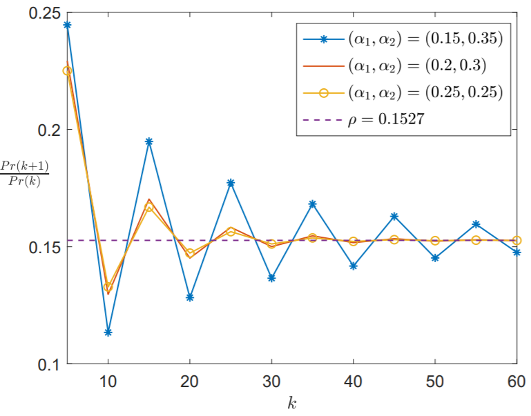
Refer to caption
Figure 10: The ratio Pr(k+1)Pr(k)𝑃𝑟𝑘1𝑃𝑟𝑘\frac{Pr(k+1)}{Pr(k)} for increasing values of k=N1+N2𝑘subscript𝑁1subscript𝑁2k=N_{1}+N_{2}.

We now focus on the stationary approximations derived through the heuristic approach in subsection 4.2. In Figure 10 we observe the ratio Pr(k+1)Pr(k)𝑃𝑟𝑘1𝑃𝑟𝑘\frac{Pr(k+1)}{Pr(k)} for increasing values of the total number of jobs in orbits, i.e., k=N1+N2𝑘subscript𝑁1subscript𝑁2k=N_{1}+N_{2}, where Pr(k)=pi,j(1)+pi,j(0)𝑃𝑟𝑘subscript𝑝𝑖𝑗1subscript𝑝𝑖𝑗0Pr(k)=p_{i,j}(1)+p_{i,j}(0) with k=i+j𝑘𝑖𝑗k=i+j, and λ0=0.04subscript𝜆00.04\lambda_{0}=0.04, λ1=λ2=0.01subscript𝜆1subscript𝜆20.01\lambda_{1}=\lambda_{2}=0.01, μ=0.44𝜇0.44\mu=0.44. It is readily seen that limkPr(k+1)Pr(k)=ρ=λ^μ^1+μ^2subscript𝑘𝑃𝑟𝑘1𝑃𝑟𝑘𝜌^𝜆subscript^𝜇1subscript^𝜇2\lim_{k\to\infty}\frac{Pr(k+1)}{Pr(k)}=\rho=\frac{\widehat{\lambda}}{\widehat{\mu}_{1}+\widehat{\mu}_{2}}. Moreover, we can observe that the more the difference α1α2subscript𝛼1subscript𝛼2\alpha_{1}-\alpha_{2} get smaller, the faster this ratio tends to ρ𝜌\rho. In other words, the asymmetry of the retrial rates affects the asymptotic behaviour.

Moreover, we can also observe that the presence of the dedicated traffic, also heavily affects the way the ratio Pr(k+1)Pr(k)𝑃𝑟𝑘1𝑃𝑟𝑘\frac{Pr(k+1)}{Pr(k)} tends to ρ𝜌\rho. In the following table, we can observe this trend for λ1=0=λ2subscript𝜆10subscript𝜆2\lambda_{1}=0=\lambda_{2}, λ0=0.06subscript𝜆00.06\lambda_{0}=0.06, μ=0.44𝜇0.44\mu=0.44, compared with the case where λ1=0.01=λ2subscript𝜆10.01subscript𝜆2\lambda_{1}=0.01=\lambda_{2}, λ0=0.04subscript𝜆00.04\lambda_{0}=0.04, μ=0.44𝜇0.44\mu=0.44; see Table 2

Table 2: Effect of dedicated traffic
Pr(k+1)Pr(k)𝑃𝑟𝑘1𝑃𝑟𝑘\frac{Pr(k+1)}{Pr(k)} for (α1,α2)=(0.15,0.35)subscript𝛼1subscript𝛼20.150.35(\alpha_{1},\alpha_{2})=(0.15,0.35) (λ0,λ1,λ2)=(0.06,0,0)subscript𝜆0subscript𝜆1subscript𝜆20.0600(\lambda_{0},\lambda_{1},\lambda_{2})=(0.06,0,0) (λ0,λ1,λ2)=(0.04,0.01,0.01)subscript𝜆0subscript𝜆1subscript𝜆20.040.010.01(\lambda_{0},\lambda_{1},\lambda_{2})=(0.04,0.01,0.01)
k=5𝑘5k=5 0.15260.15260.1526 0.24460.24460.2446
k=15𝑘15k=15 0.15270.15270.1527 0.19480.19480.1948
k=35𝑘35k=35 0.15270.15270.1527 0.16830.16830.1683
k=55𝑘55k=55 0.15270.15270.1527 0.15960.15960.1596
Pr(k+1)Pr(k)𝑃𝑟𝑘1𝑃𝑟𝑘\frac{Pr(k+1)}{Pr(k)} for (α1,α2)=(0.25,0.25)subscript𝛼1subscript𝛼20.250.25(\alpha_{1},\alpha_{2})=(0.25,0.25) (λ0,λ1,λ2)=(0.06,0,0)subscript𝜆0subscript𝜆1subscript𝜆20.0600(\lambda_{0},\lambda_{1},\lambda_{2})=(0.06,0,0) (λ0,λ1,λ2)=(0.04,0.01,0.01)subscript𝜆0subscript𝜆1subscript𝜆20.040.010.01(\lambda_{0},\lambda_{1},\lambda_{2})=(0.04,0.01,0.01)
k=5𝑘5k=5 0.15270.15270.1527 0.2250.2250.225
k=15𝑘15k=15 0.15270.15270.1527 0.16690.16690.1669
k=35𝑘35k=35 0.15270.15270.1527 0.15380.15380.1538
k=55𝑘55k=55 0.15270.15270.1527 0.15270.15270.1527

We observe, that in case of no dedicated traffic the convergence of the ratio Pr(k+1)Pr(k)𝑃𝑟𝑘1𝑃𝑟𝑘\frac{Pr(k+1)}{Pr(k)} to ρ𝜌\rho is really faster compared with the case where we assumed dedicated traffic. Note that in these scenarios we have assumed that the total arrival rate is fixed and equal to λ=0.06𝜆0.06\lambda=0.06, so that ρ=0.1527𝜌0.1527\rho=0.1527 is fixed in both cases.

Moreover, we note when ρ𝜌\rho increases, the ratio Pr(k+1)Pr(k)𝑃𝑟𝑘1𝑃𝑟𝑘\frac{Pr(k+1)}{Pr(k)} tends to ρ𝜌\rho very fast (from k10𝑘10k\geq 10 the ratio is very close to ρ𝜌\rho), as shown in Figure 11, where λ0=0.19subscript𝜆00.19\lambda_{0}=0.19, λ1=λ1=0.01subscript𝜆1subscript𝜆10.01\lambda_{1}=\lambda_{1}=0.01 μ=0.44𝜇0.44\mu=0.44 (in the case of no dedicated traffic, we assumed λ1=λ2=0subscript𝜆1subscript𝜆20\lambda_{1}=\lambda_{2}=0, λ0=0.21subscript𝜆00.21\lambda_{0}=0.21).

Refer to caption
Figure 11: The ratio Pr(k+1)Pr(k)𝑃𝑟𝑘1𝑃𝑟𝑘\frac{Pr(k+1)}{Pr(k)} for increasing values of k=N1+N2𝑘subscript𝑁1subscript𝑁2k=N_{1}+N_{2}.

7 Conclusion and future work

In this work, we introduced the generalized join the shortest queue system with retrials and two infinite capacity orbit queues. Three independent streams of jobs, namely a smart, and two dedicated streams, flow into a single server service system, which can hold at most one job. Blocked smart jobs join the shortest orbit queue, while blocked jobs from the dedicated streams join their corresponding orbit queue. We remind that the system is described as a Markov modulated two-dimensional random walk, but this kind of modulation allowed for a completely tractable analysis.

We establish the geometric tail asymptotics along the minimum direction for a fixed value of the difference among orbit queue lengths. Moreover, we apply a heuristic approach to obtain stationary approximations of the number of the joint orbit queue length distribution, which are accurate when one of the orbit queue lengths is large, and thus agreed with the asymptotic analysis. We have shown that even though the exact solution to the problem may be quite complicated, the asymptotic expansions of pi,j(k)subscript𝑝𝑖𝑗𝑘p_{i,j}(k) are relatively simple and clearly indicate the dependence of the stationary distribution on the parameters of the model.

We also cope with the stability condition, and based on the stability of the censored chain on the busy states along with extensive simulation experiments, we conjecture that the ergodicity conditions of the censored chain coincide with those of the original model. We postpone the formal proof of this conjecture in a future work. We also leave as a future work the complete investigation of the tail decay rate problem. More precisely, we proved the exact geometric decay under specific conditions given in Theorem 4.1 (which are similar to those given in [15]), but it is still an open problem the investigation of the decay rates when these conditions collapse.

Finally, simulation experiments indicate that in heavy traffic (i.e., ρ1𝜌1\rho\to 1) and when λ0>|λ1λ2|subscript𝜆0subscript𝜆1subscript𝜆2\lambda_{0}>|\lambda_{1}-\lambda_{2}|, α1=α2subscript𝛼1subscript𝛼2\alpha_{1}=\alpha_{2}, our system exhibits a state-space collapse behaviour; see Figure 12 (right). It seems that when the first condition fails, our model does not retain this behaviour; see Figure 12 (left), where λ1>λ0>λ2subscript𝜆1subscript𝜆0subscript𝜆2\lambda_{1}>\lambda_{0}>\lambda_{2}, and λ0<|λ1λ2|subscript𝜆0subscript𝜆1subscript𝜆2\lambda_{0}<|\lambda_{1}-\lambda_{2}| (i.e., the impact of dedicated traffic for orbit queue 1 is very crucial). Moreover, it also seems that the condition α1=α2subscript𝛼1subscript𝛼2\alpha_{1}=\alpha_{2} is not crucial (see Figure 9 (left)).

This means that in heavy-traffic and under these conditions, our load balancing scheme collapses to a one-dimensional line where all the orbit queue lengths are equal. A similar result was proven for the GJSQ system without retrials in the seminal paper [16]. State-space collapse occurs because the smart traffic flow dominates over the dedicated traffic flows and “forces” the two orbit queues to be equal. Thus, it seams that in the heavy traffic regime the sum of the orbit queue lengths can be approximated by the reference system described at the end of subsection 4.1. The reference system behaves as if there is only a single orbit queue with all the “servers” (i.e., the retrial servers) pooled together as an aggregated “server” (in standard JSQ systems this is called complete resource pooling). This result implies that under specific conditions, GJSOQ is asymptotically optimal, i.e., heavy-traffic delay optimal, since the response time in the pooled single-orbit system is stochastically less than that of a typical load balancing system, i.e. the reference system seams to serve as a lower bound (in the stochastic sense) on the total orbit queue length of the original model. In a future study we plan to prove formally this justification.
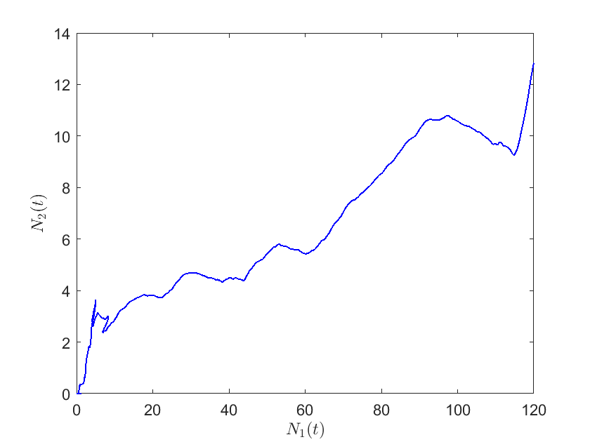
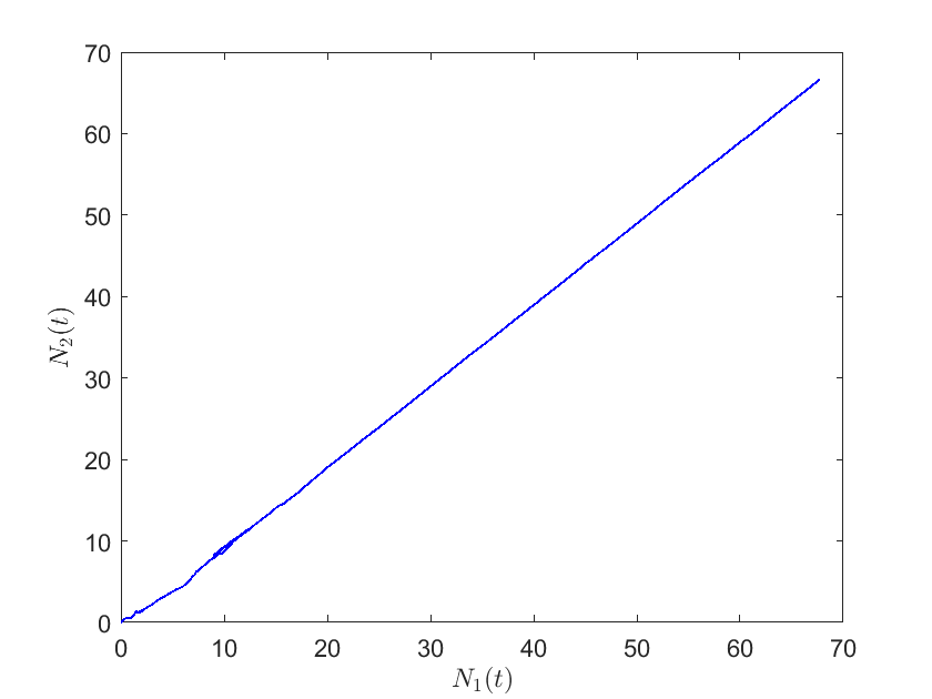
Refer to caption
Refer to caption
Figure 12: Orbit dynamics for ρ1𝜌1\rho\to 1 when λ0<|λ1λ2|subscript𝜆0subscript𝜆1subscript𝜆2\lambda_{0}<|\lambda_{1}-\lambda_{2}| (left), and when λ0>|λ1λ2|subscript𝜆0subscript𝜆1subscript𝜆2\lambda_{0}>|\lambda_{1}-\lambda_{2}| (right).

Acknowledgements

I would like to thank the Editors and the reviewers for the insightful remarks, which helped to improve the original exposition.
Competing interests: The author declare none.

References

  • [1] I. Adan, G.-J. van Houtum, and J. van der Wal. Upper and lower bounds for the waiting time in the symmetric shortest queue system. Annals of Operations Research, 48(2):197–217, 1994.
  • [2] I. J. B. F. Adan, O. J. Boxma, and J. A. C. Resing. Queueing models with multiple waiting lines. Queueing Systems, 37(1-3):65–98, 2001.
  • [3] I. J. B. F. Adan, S. Kapodistria, and J. S. H. van Leeuwaarden. Erlang arrivals joining the shorter queue. Queueing Systems, 74(2-3):273–302, 2013.
  • [4] I. J. B. F. Adan, J. Wessels, and W. Zijm. A compensation approach for two-dimentional Markov processes. Advances in Applied Probability, 25(4):783–817, 1993.
  • [5] I. J. B. F. Adan, J. Wessels, and W. H. Zijm. Analysis of the symmetric shortest queue problem. Stochastic Models, 6(1):691–713, 1990.
  • [6] I. J. B. F. Adan, J. Wessels, and W. H. M. Zijm. Analysis of the asymmetric shortest queue problem. Queueing Systems, 8(1):1–58, 1991.
  • [7] J. R. Artalejo and A. Gómez-Corral. Retrial Queueing Systems: A Computational Approach. Springer, Berlin, Heidelberg, 2008.
  • [8] J. P. C. Blanc. A note on waiting times in systems with queues in parallel. Journal of Applied Probability, 24(2):540–546, 1987.
  • [9] J. Cohen and O. Boxma. Boundary value problems in queueing systems analysis. North Holland Publishing Company, Amsterdam, Netherlands, 1983.
  • [10] I. Dimitriou. A queueing system for modeling cooperative wireless networks with coupled relay nodes and synchronized packet arrivals. Performance Evaluation, 114:16–31, 2017.
  • [11] I. Dimitriou. Analysis of the symmetric join the shortest orbit queue. Operations Research Letters, 49(1):23 – 29, 2021.
  • [12] G. Falin and J. Templeton. Retrial Queues. Chapman & Hall, London, 1997.
  • [13] G. Fayolle, R. Iasnogorodski, and V. Malyshev. Random walks in the quarter-plane: Algebraic methods, boundary value problems, applications to queueing systems and analytic combinatorics. Springer-Verlag, Berlin, 2017.
  • [14] G. Fayolle, V. A. Malyshev, and M. Menshikov. Topics in the constructive theory of countable Markov chains. Cambridge university press, 1995.
  • [15] R. D. Foley and D. R. McDonald. Join the shortest queue: stability and exact asymptotics. Ann. Appl. Probab., 11(3):569–607, 08 2001.
  • [16] G. Foschini and J. Salz. A basic dynamic routing problem and diffusion. IEEE Transactions on Communications, 26(3):320–327, 1978.
  • [17] I. Gertsbakh. The shorter queue problem: A numerical study using the matrix-geometric solution. European Journal of Operational Research, 15(3):374 – 381, 1984.
  • [18] F. A. Haight. Two queues in parallel. Biometrika, 45(3/4):401–410, 1958.
  • [19] S. Kapodistria and Z. Palmowski. Matrix geometric approach for random walks: Stability condition and equilibrium distribution. Stochastic Models, 33(4):572–597, 2017.
  • [20] J. G. Kemeny, J. L. Snell, and A. W. Knapp. Denumerable Markov Chains. Springer, New York, USA, 2nd edition, 1976.
  • [21] J. F. C. Kingman. Two similar queues in parallel. Ann. Math. Statist., 32(4):1314–1323, 12 1961.
  • [22] C. Knessl, B. Matkowsky, Z. Schuss, and C. Tier. Two parallel queues with dynamic routing. IEEE Transactions on Communications, 34(12):1170–1175, 1986.
  • [23] M. Kobayashi, Y. Sakuma, and M. Miyazawa. Join the shortest queue among k parallel queues: tail asymptotics of its stationary distribution. Queueing Systems, 74:303–332, 2013.
  • [24] I. Kurkova. A load-balanced network with two servers. Queueing Systems, 37:379–389, 2001.
  • [25] I. A. Kurkova and Y. M. Suhov. Malyshev’s theory and JS-queues. Asymptotics of stationary probabilities. Ann. Appl. Probab., 13(4):1313–1354, 11 2003.
  • [26] H. Li, M. Miyazawa, and Y. Zhao. Geometric decay in a QBD process with countable background states with applications to a join-the-shortest-queue model. Stochastic Models, 23(3):413–438, 2007.
  • [27] V. A. Malyshev. Asymptotic behavior of the stationary probabilities for two-dimensional positive random walks. Sibirsk. Mat. Ž., 14:156–169, 238, 1973.
  • [28] S. Meyn and R. L. Tweedie. Markov Chains and Stochastic Stability. Cambridge University Press, USA, 2nd edition, 2009.
  • [29] M. Miyazawa. Tail decay rates in double QBD processes and related reflected random walks. Mathematics of Operations Research, 34(3):547–575, 2009.
  • [30] M. Miyazawa. Two Sided DQBD Process and Solutions to the Tail Decay Rate Problem and Their Applications to the Generalized Join Shortest Queue, pages 3–33. Springer New York, New York, NY, 2009.
  • [31] M. Miyazawa. Light tail asymptotics in multidimensional reflecting processes for queueing networks. TOP, 19(2):233–299, Dec 2011.
  • [32] M. F. Neuts. Matrix-geometric solutions in stochastic models: an algorithmic approach. Johns Hopkins University Press Baltimore, 1981.
  • [33] T. Ozawa. Asymptotics for the stationary distribution in a discrete-time two-dimensional quasi-birth-and-death process. Queueing Systems, 74(2):109–149, Jun 2013.
  • [34] T. Ozawa. Stability condition of a two-dimensional QBD process and its application to estimation of efficiency for two-queue models. Performance Evaluation, 130:101–118, 2019.
  • [35] N. Pappas, M. Kountouris, A. Ephremides, and A. Traganitis. Relay-assisted multiple access with full-duplex multi-packet reception. IEEE Transactions on Wireless Communications, 14(7):3544–3558, July 2015.
  • [36] A. Puhalskii and A. Vladimirov. A large deviation principle for join the shortest queue. Mathematics of Operations Research, 32(3):700–710, 2007.
  • [37] B. M. Rao and M. J. M. Posner. Algorithmic and approximation analyses of the shorter queue model. Naval Research Logistics, 34(3):381–398, 1987.
  • [38] Y. Sakuma. Asymptotic behavior for MAP/PH/c queue with shortest queue discipline and jockeying. Operations Research Letters, 38(1):7–10, 2010.
  • [39] Y. Sakuma, M. Miyazawa, and Y. Zhao. Decay rate for a PH/M/2 queue with shortest queue discipline. Queueing Systems, 53:189–201, 2006.
  • [40] Y. Takahashi, K. Fujimoto, and N. Makimoto. Geometric decay of the steady-state probabilities in a quasi-birth-and-death process with a countable number of phases. Stochastic Models, 17(1):1–24, 2001.
  • [41] S. Turner. Large deviations for join the shorter queue, pages 95–108. AMS, 2000.
  • [42] S. R. E. Turner. A join the shorter queue model in heavy traffic. Journal of Applied Probability, 37(1):212–223, 2000.
  • [43] Y. Q. Zhao and D. Liu. The censored markov chain and the best augmentation. Journal of Applied Probability, 33(3):623–629, 1996.

Appendix A Proof of Lemma 1

Denote by (Mi(rk),Mj(rk))superscriptsubscript𝑀𝑖subscript𝑟𝑘superscriptsubscript𝑀𝑗subscript𝑟𝑘(M_{i}^{(r_{k})},M_{j}^{(r_{k})}) the mean jump vectors in angle rksubscript𝑟𝑘r_{k}, k=1,2,𝑘12k=1,2, and by (Mi(h),Mj(h))superscriptsubscript𝑀𝑖superscriptsubscript𝑀𝑗(M_{i}^{(h)},M_{j}^{(h)}), (Mi(v),Mj(v))superscriptsubscript𝑀𝑖𝑣superscriptsubscript𝑀𝑗𝑣(M_{i}^{(v)},M_{j}^{(v)}) the mean jump vectors in rays hh and v𝑣v, respectively. Then,

Mi(r1)=λ1μ^1λ+α1+α2,Mj(r1)=λ0+λ2μ^2λ+α1+α2,Mi(r2)=λ0+λ1μ^1λ+α1+α2,Mj(r2)=λ2μ^2λ+α1+α2,Mi(h)=λ1μ^1λ+α1,Mj(h)=λ0+λ2,Mi(v)=λ0+λ1,Mj(h)=λ2μ^2λ+α2.superscriptsubscript𝑀𝑖subscript𝑟1absentsubscript𝜆1subscript^𝜇1𝜆subscript𝛼1subscript𝛼2missing-subexpressionsuperscriptsubscript𝑀𝑗subscript𝑟1absentsubscript𝜆0subscript𝜆2subscript^𝜇2𝜆subscript𝛼1subscript𝛼2superscriptsubscript𝑀𝑖subscript𝑟2absentsubscript𝜆0subscript𝜆1subscript^𝜇1𝜆subscript𝛼1subscript𝛼2missing-subexpressionsuperscriptsubscript𝑀𝑗subscript𝑟2absentsubscript𝜆2subscript^𝜇2𝜆subscript𝛼1subscript𝛼2superscriptsubscript𝑀𝑖absentsubscript𝜆1subscript^𝜇1𝜆subscript𝛼1missing-subexpressionsuperscriptsubscript𝑀𝑗absentsubscript𝜆0subscript𝜆2superscriptsubscript𝑀𝑖𝑣absentsubscript𝜆0subscript𝜆1missing-subexpressionsuperscriptsubscript𝑀𝑗absentsubscript𝜆2subscript^𝜇2𝜆subscript𝛼2\begin{array}[]{rlcrl}M_{i}^{(r_{1})}=&\lambda_{1}-\frac{\widehat{\mu}_{1}}{\lambda+\alpha_{1}+\alpha_{2}},&&M_{j}^{(r_{1})}=&\lambda_{0}+\lambda_{2}-\frac{\widehat{\mu}_{2}}{\lambda+\alpha_{1}+\alpha_{2}},\\ M_{i}^{(r_{2})}=&\lambda_{0}+\lambda_{1}-\frac{\widehat{\mu}_{1}}{\lambda+\alpha_{1}+\alpha_{2}},&&M_{j}^{(r_{2})}=&\lambda_{2}-\frac{\widehat{\mu}_{2}}{\lambda+\alpha_{1}+\alpha_{2}},\\ M_{i}^{(h)}=&\lambda_{1}-\frac{\widehat{\mu}_{1}}{\lambda+\alpha_{1}},&&M_{j}^{(h)}=&\lambda_{0}+\lambda_{2},\\ M_{i}^{(v)}=&\lambda_{0}+\lambda_{1},&&M_{j}^{(h)}=&\lambda_{2}-\frac{\widehat{\mu}_{2}}{\lambda+\alpha_{2}}.\end{array}

The mean jump vector from ray d𝑑d equals 12(Mi(r1)+Mi(r2),Mj(r1)+Mj(r2))12superscriptsubscript𝑀𝑖subscript𝑟1superscriptsubscript𝑀𝑖subscript𝑟2superscriptsubscript𝑀𝑗subscript𝑟1superscriptsubscript𝑀𝑗subscript𝑟2\frac{1}{2}(M_{i}^{(r_{1})}+M_{i}^{(r_{2})},M_{j}^{(r_{1})}+M_{j}^{(r_{2})}), while Mi(r1)+Mj(r1)=Mi(r2)+Mj(r2)=λμ^1+μ^2λ+α1+α2=λ^μ^1μ^2λ+α1+α2superscriptsubscript𝑀𝑖subscript𝑟1superscriptsubscript𝑀𝑗subscript𝑟1superscriptsubscript𝑀𝑖subscript𝑟2superscriptsubscript𝑀𝑗subscript𝑟2𝜆subscript^𝜇1subscript^𝜇2𝜆subscript𝛼1subscript𝛼2^𝜆subscript^𝜇1subscript^𝜇2𝜆subscript𝛼1subscript𝛼2M_{i}^{(r_{1})}+M_{j}^{(r_{1})}=M_{i}^{(r_{2})}+M_{j}^{(r_{2})}=\lambda-\frac{\widehat{\mu}_{1}+\widehat{\mu}_{2}}{\lambda+\alpha_{1}+\alpha_{2}}=\frac{\widehat{\lambda}-\widehat{\mu}_{1}-\widehat{\mu}_{2}}{\lambda+\alpha_{1}+\alpha_{2}}.

Let us first focus on the sufficient part. We use the well known Foster’s criterion [14, Theorem 2.3.3], i.e., the Markov chain {X(n);n0}𝑋𝑛𝑛0\{X(n);n\geq 0\} is ergodic iff there exists a positive function f(i,j)𝑓𝑖𝑗f(i,j) on +2superscriptsubscript2\mathbb{Z}_{+}^{2}, ϵ>0italic-ϵ0\epsilon>0 and a finite set A+2𝐴superscriptsubscript2A\in\mathbb{Z}_{+}^{2} such that

E(f(i+θi,j+θj))f(i,j)<ϵ,(x,y)+2/A,formulae-sequence𝐸𝑓𝑖subscript𝜃𝑖𝑗subscript𝜃𝑗𝑓𝑖𝑗italic-ϵ𝑥𝑦superscriptsubscript2𝐴E(f(i+\theta_{i},j+\theta_{j}))-f(i,j)<-\epsilon,\,\,(x,y)\in\mathbb{Z}_{+}^{2}/A, (A.1)

where (θi,θj)subscript𝜃𝑖subscript𝜃𝑗(\theta_{i},\theta_{j}) is a random vector distributed as a one-step jump of the chain X(n)𝑋𝑛X(n) from the state (i,j)𝑖𝑗(i,j).

We first assume that assertion 1 in Theorem 1 holds, i.e., λ^1<μ^1subscript^𝜆1subscript^𝜇1\widehat{\lambda}_{1}<\widehat{\mu}_{1}, λ^2<μ^2subscript^𝜆2subscript^𝜇2\widehat{\lambda}_{2}<\widehat{\mu}_{2}, λ^<μ^1+μ^2^𝜆subscript^𝜇1subscript^𝜇2\widehat{\lambda}<\widehat{\mu}_{1}+\widehat{\mu}_{2}. Consider the function f(i,j)=i2+j2𝑓𝑖𝑗superscript𝑖2superscript𝑗2f(i,j)=\sqrt{i^{2}+j^{2}}. Then, simple manipulation yields

E(f(i+θi,j+θj))f(i,j)=xE(θi)+yE(θj)f(i,j)+o(1),as i2+j2.formulae-sequence𝐸𝑓𝑖subscript𝜃𝑖𝑗subscript𝜃𝑗𝑓𝑖𝑗𝑥𝐸subscript𝜃𝑖𝑦𝐸subscript𝜃𝑗𝑓𝑖𝑗𝑜1as superscript𝑖2superscript𝑗2E(f(i+\theta_{i},j+\theta_{j}))-f(i,j)=\frac{xE(\theta_{i})+yE(\theta_{j})}{f(i,j)}+o(1),\,\text{as }i^{2}+j^{2}\to\infty.

Then, in angle r1subscript𝑟1r_{1} we have E(θi)=Mi(r1)=λ^1μ^1λ+α1+α2<0𝐸subscript𝜃𝑖superscriptsubscript𝑀𝑖subscript𝑟1subscript^𝜆1subscript^𝜇1𝜆subscript𝛼1subscript𝛼20E(\theta_{i})=M_{i}^{(r_{1})}=\frac{\widehat{\lambda}_{1}-\widehat{\mu}_{1}}{\lambda+\alpha_{1}+\alpha_{2}}<0, and E(θi)+E(θj)=Mi(r1)+Mj(r1)=λ^μ^1μ^2λ+α1+α2<0𝐸subscript𝜃𝑖𝐸subscript𝜃𝑗superscriptsubscript𝑀𝑖subscript𝑟1superscriptsubscript𝑀𝑗subscript𝑟1^𝜆subscript^𝜇1subscript^𝜇2𝜆subscript𝛼1subscript𝛼20E(\theta_{i})+E(\theta_{j})=M_{i}^{(r_{1})}+M_{j}^{(r_{1})}=\frac{\widehat{\lambda}-\widehat{\mu}_{1}-\widehat{\mu}_{2}}{\lambda+\alpha_{1}+\alpha_{2}}<0. Moreover, in r1subscript𝑟1r_{1}

E(f(i+θi,j+θj))f(i,j)j(E(θi)+E(θj))j2+o(1)<ϵ1𝐸𝑓𝑖subscript𝜃𝑖𝑗subscript𝜃𝑗𝑓𝑖𝑗𝑗𝐸subscript𝜃𝑖𝐸subscript𝜃𝑗𝑗2𝑜1subscriptitalic-ϵ1E(f(i+\theta_{i},j+\theta_{j}))-f(i,j)\leq\frac{j(E(\theta_{i})+E(\theta_{j}))}{j\sqrt{2}}+o(1)<-\epsilon_{1}

for ϵ1>0subscriptitalic-ϵ10\epsilon_{1}>0 as i2+j2superscript𝑖2superscript𝑗2i^{2}+j^{2}\to\infty.

For (i,j)𝑖𝑗(i,j) in ray hh, the condition λ^1<μ^1subscript^𝜆1subscript^𝜇1\widehat{\lambda}_{1}<\widehat{\mu}_{1}, i.e.,formulae-sequence𝑖𝑒i.e., Mi(r1)<0superscriptsubscript𝑀𝑖subscript𝑟10M_{i}^{(r_{1})}<0, implies Mi(h)<0superscriptsubscript𝑀𝑖0M_{i}^{(h)}<0, since

Mi(h)=Mi(r1)+μ^1(1λ+α1+α21λ+α1)=Mi(r1)α2μ^1(λ+α1)(λ+α1+α2)<0.superscriptsubscript𝑀𝑖superscriptsubscript𝑀𝑖subscript𝑟1subscript^𝜇11𝜆subscript𝛼1subscript𝛼21𝜆subscript𝛼1superscriptsubscript𝑀𝑖subscript𝑟1subscript𝛼2subscript^𝜇1𝜆subscript𝛼1𝜆subscript𝛼1subscript𝛼20M_{i}^{(h)}=M_{i}^{(r_{1})}+\widehat{\mu}_{1}(\frac{1}{\lambda+\alpha_{1}+\alpha_{2}}-\frac{1}{\lambda+\alpha_{1}})=M_{i}^{(r_{1})}-\frac{\alpha_{2}\widehat{\mu}_{1}}{(\lambda+\alpha_{1})(\lambda+\alpha_{1}+\alpha_{2})}<0.

Therefore,

E(f(i+θi,j+θj))f(i,j)iMi(h)i+o(1)<ϵ2𝐸𝑓𝑖subscript𝜃𝑖𝑗subscript𝜃𝑗𝑓𝑖𝑗𝑖superscriptsubscript𝑀𝑖𝑖𝑜1subscriptitalic-ϵ2E(f(i+\theta_{i},j+\theta_{j}))-f(i,j)\leq\frac{iM_{i}^{(h)}}{i}+o(1)<-\epsilon_{2}

for ϵ2>0subscriptitalic-ϵ20\epsilon_{2}>0 as i2superscript𝑖2i^{2}\to\infty. The case for angle r2subscript𝑟2r_{2} and ray v𝑣v are symmetric to those for r1subscript𝑟1r_{1} and hh, respectively, thus, (A.1) is verified similarly. The case for the ray d𝑑d, i.e., i=j𝑖𝑗i=j is treated similarly. Indeed, having in mind that (E(θi),E(θj))=12(Mi(r1)+Mi(r2),Mj(r1)+Mj(r2))𝐸subscript𝜃𝑖𝐸subscript𝜃𝑗12superscriptsubscript𝑀𝑖subscript𝑟1superscriptsubscript𝑀𝑖subscript𝑟2superscriptsubscript𝑀𝑗subscript𝑟1superscriptsubscript𝑀𝑗subscript𝑟2(E(\theta_{i}),E(\theta_{j}))=\frac{1}{2}(M_{i}^{(r_{1})}+M_{i}^{(r_{2})},M_{j}^{(r_{1})}+M_{j}^{(r_{2})}), (A.1) reads

E(f(i+θi,j+θj))f(i,j)=i2E(θi)i2+o(1)=Mi(r1)+Mj(r1)2+o(1)<ϵ3,as i.𝐸𝑓𝑖subscript𝜃𝑖𝑗subscript𝜃𝑗𝑓𝑖𝑗absentformulae-sequence𝑖2𝐸subscript𝜃𝑖𝑖2𝑜1superscriptsubscript𝑀𝑖subscript𝑟1superscriptsubscript𝑀𝑗subscript𝑟12𝑜1subscriptitalic-ϵ3as 𝑖\begin{array}[]{rl}E(f(i+\theta_{i},j+\theta_{j}))-f(i,j)=&\frac{i2E(\theta_{i})}{i\sqrt{2}}+o(1)=\frac{M_{i}^{(r_{1})}+M_{j}^{(r_{1})}}{\sqrt{2}}+o(1)<-\epsilon_{3},\,\text{as }i\to\infty.\end{array}

Assume now that assertion 2 in Theorem 1 holds: λ^1μ^1subscript^𝜆1subscript^𝜇1\widehat{\lambda}_{1}\geq\widehat{\mu}_{1}, λ^2<μ^2subscript^𝜆2subscript^𝜇2\widehat{\lambda}_{2}<\widehat{\mu}_{2}, and Mi(r1)Mj(h)Mi(h)Mj(r1)<0f1<0superscriptsubscript𝑀𝑖subscript𝑟1superscriptsubscript𝑀𝑗superscriptsubscript𝑀𝑖superscriptsubscript𝑀𝑗subscript𝑟10subscript𝑓10M_{i}^{(r_{1})}M_{j}^{(h)}-M_{i}^{(h)}M_{j}^{(r_{1})}<0\Leftrightarrow f_{1}<0. In such a case the following hold:

Mi(r2)>Mi(r1)0,Mj(r2)<Mj(r1)<0,Mi(r1)Mj(h)<Mi(h)Mj(r1)Mi(h)<Mi(r1)Mj(r1)Mj(h)<0(since Mj(r1)<0),Mj(v)=Mj(r2)α1μ^2(λ+α1)(λ+α1+α2)<0.superscriptsubscript𝑀𝑖subscript𝑟2absentsuperscriptsubscript𝑀𝑖subscript𝑟10superscriptsubscript𝑀𝑗subscript𝑟2absentsuperscriptsubscript𝑀𝑗subscript𝑟10superscriptsubscript𝑀𝑖subscript𝑟1superscriptsubscript𝑀𝑗absentsuperscriptsubscript𝑀𝑖superscriptsubscript𝑀𝑗subscript𝑟1superscriptsubscript𝑀𝑖superscriptsubscript𝑀𝑖subscript𝑟1superscriptsubscript𝑀𝑗subscript𝑟1superscriptsubscript𝑀𝑗0since superscriptsubscript𝑀𝑗subscript𝑟10superscriptsubscript𝑀𝑗𝑣absentsuperscriptsubscript𝑀𝑗subscript𝑟2subscript𝛼1subscript^𝜇2𝜆subscript𝛼1𝜆subscript𝛼1subscript𝛼20\begin{array}[]{rl}M_{i}^{(r_{2})}>&M_{i}^{(r_{1})}\geq 0,\\ M_{j}^{(r_{2})}<&M_{j}^{(r_{1})}<0,\\ M_{i}^{(r_{1})}M_{j}^{(h)}<&M_{i}^{(h)}M_{j}^{(r_{1})}\Rightarrow M_{i}^{(h)}<\frac{M_{i}^{(r_{1})}}{M_{j}^{(r_{1})}}M_{j}^{(h)}<0\,\,\,\,(\text{since }M_{j}^{(r_{1})}<0),\\ M_{j}^{(v)}=&M_{j}^{(r_{2})}-\frac{\alpha_{1}\widehat{\mu}_{2}}{(\lambda+\alpha_{1})(\lambda+\alpha_{1}+\alpha_{2})}<0.\end{array}

Note also that Mi(r1)Mj(h)Mi(h)Mj(r1)<0superscriptsubscript𝑀𝑖subscript𝑟1superscriptsubscript𝑀𝑗superscriptsubscript𝑀𝑖superscriptsubscript𝑀𝑗subscript𝑟10M_{i}^{(r_{1})}M_{j}^{(h)}-M_{i}^{(h)}M_{j}^{(r_{1})}<0 is equivalent to λ1<μ1λ0+λ2μ~2(μ1μ~1)subscript𝜆1superscriptsubscript𝜇1subscript𝜆0subscript𝜆2subscript~𝜇2superscriptsubscript𝜇1subscript~𝜇1\lambda_{1}<\mu_{1}^{*}-\frac{\lambda_{0}+\lambda_{2}}{\tilde{\mu}_{2}}(\mu_{1}^{*}-\tilde{\mu}_{1}), where μ~i=μ^iλ+α1+α2subscript~𝜇𝑖subscript^𝜇𝑖𝜆subscript𝛼1subscript𝛼2\tilde{\mu}_{i}=\frac{\widehat{\mu}_{i}}{\lambda+\alpha_{1}+\alpha_{2}}, i=1,2𝑖12i=1,2, and μ1=μ^1λ+α1superscriptsubscript𝜇1subscript^𝜇1𝜆subscript𝛼1\mu_{1}^{*}=\frac{\widehat{\mu}_{1}}{\lambda+\alpha_{1}}. Then,

Mi(r1)+Mj(r2)=λμ~1μ~2<λ1μ1+λ0+λ2μ~2(μ1μ~1)<0.superscriptsubscript𝑀𝑖subscript𝑟1superscriptsubscript𝑀𝑗subscript𝑟2𝜆subscript~𝜇1subscript~𝜇2subscript𝜆1superscriptsubscript𝜇1subscript𝜆0subscript𝜆2subscript~𝜇2superscriptsubscript𝜇1subscript~𝜇10missing-subexpression\begin{array}[]{rl}M_{i}^{(r_{1})}+M_{j}^{(r_{2})}=\lambda-\tilde{\mu}_{1}-\tilde{\mu}_{2}<\lambda_{1}-\mu_{1}^{*}+\frac{\lambda_{0}+\lambda_{2}}{\tilde{\mu}_{2}}(\mu_{1}^{*}-\tilde{\mu}_{1})<0.\end{array}

Indeed,

λμ~1μ~2<λ1μ1+λ0+λ2μ~2(μ1μ~1)(λ0+λ2μ~21)(μ~2+μ~1μ1)<0.𝜆subscript~𝜇1subscript~𝜇2subscript𝜆1superscriptsubscript𝜇1subscript𝜆0subscript𝜆2subscript~𝜇2superscriptsubscript𝜇1subscript~𝜇1absentsubscript𝜆0subscript𝜆2subscript~𝜇21subscript~𝜇2subscript~𝜇1superscriptsubscript𝜇10\begin{array}[]{rl}\lambda-\tilde{\mu}_{1}-\tilde{\mu}_{2}<\lambda_{1}-\mu_{1}^{*}+\frac{\lambda_{0}+\lambda_{2}}{\tilde{\mu}_{2}}(\mu_{1}^{*}-\tilde{\mu}_{1})\Leftrightarrow&(\frac{\lambda_{0}+\lambda_{2}}{\tilde{\mu}_{2}}-1)(\tilde{\mu}_{2}+\tilde{\mu}_{1}-\mu_{1}^{*})<0.\end{array}

Since Mj(r1)=λ0+λ2μ~2<0superscriptsubscript𝑀𝑗subscript𝑟1subscript𝜆0subscript𝜆2subscript~𝜇20M_{j}^{(r_{1})}=\lambda_{0}+\lambda_{2}-\tilde{\mu}_{2}<0, it suffices to show that μ~2+μ~1μ1>0subscript~𝜇2subscript~𝜇1superscriptsubscript𝜇10\tilde{\mu}_{2}+\tilde{\mu}_{1}-\mu_{1}^{*}>0. Indeed, simple calculations yields μ~2+μ~1μ1=λμ~2λ+α1>0subscript~𝜇2subscript~𝜇1superscriptsubscript𝜇1𝜆subscript~𝜇2𝜆subscript𝛼10\tilde{\mu}_{2}+\tilde{\mu}_{1}-\mu_{1}^{*}=\frac{\lambda\tilde{\mu}_{2}}{\lambda+\alpha_{1}}>0. Thus, Mi(r1)+Mj(r1)=Mi(r2)+Mj(r2)<0.superscriptsubscript𝑀𝑖subscript𝑟1superscriptsubscript𝑀𝑗subscript𝑟1superscriptsubscript𝑀𝑖subscript𝑟2superscriptsubscript𝑀𝑗subscript𝑟20M_{i}^{(r_{1})}+M_{j}^{(r_{1})}=M_{i}^{(r_{2})}+M_{j}^{(r_{2})}<0.

We construct the function f(i,j)=ki2+lj2+wij𝑓𝑖𝑗𝑘superscript𝑖2𝑙superscript𝑗2𝑤𝑖𝑗f(i,j)=\sqrt{ki^{2}+lj^{2}+wij} with k,l>0𝑘𝑙0k,l>0, kl>w2/4𝑘𝑙superscript𝑤24kl>w^{2}/4, satisfying (A.1). We first choose k,w>0𝑘𝑤0k,w>0 such that

2kMi(r1)+lMj(r1)<0,2kMi(h)+lMj(h)<0,2𝑘superscriptsubscript𝑀𝑖subscript𝑟1𝑙superscriptsubscript𝑀𝑗subscript𝑟1absent02𝑘superscriptsubscript𝑀𝑖𝑙superscriptsubscript𝑀𝑗absent0\begin{array}[]{rl}2kM_{i}^{(r_{1})}+lM_{j}^{(r_{1})}<&0,\\ 2kM_{i}^{(h)}+lM_{j}^{(h)}<&0,\end{array}

or equivalently

Mj(r1)Mi(r1)<2kl<Mj(h)Mi(h),superscriptsubscript𝑀𝑗subscript𝑟1superscriptsubscript𝑀𝑖subscript𝑟12𝑘𝑙superscriptsubscript𝑀𝑗superscriptsubscript𝑀𝑖\frac{M_{j}^{(r_{1})}}{M_{i}^{(r_{1})}}<-\frac{2k}{l}<\frac{M_{j}^{(h)}}{M_{i}^{(h)}},

which is possible under the assumption Mi(r1)Mj(h)Mi(h)Mj(r1)<0superscriptsubscript𝑀𝑖subscript𝑟1superscriptsubscript𝑀𝑗superscriptsubscript𝑀𝑖superscriptsubscript𝑀𝑗subscript𝑟10M_{i}^{(r_{1})}M_{j}^{(h)}-M_{i}^{(h)}M_{j}^{(r_{1})}<0. Next, take l>w2/(4l)𝑙superscript𝑤24𝑙l>w^{2}/(4l) sufficiently large. Then due to the inequalities we derived above, we ensure that

2kMi(r1)+w(Mi(r1)+Mj(r1))+2lMj(r1)<0,wMi(r2)+2kMj(r2)<0,2kMi(r2)+w(Mi(r2)+Mj(r2))+2lMj(r2)<0,wMi(v)+2kMj(v)<0.2𝑘superscriptsubscript𝑀𝑖subscript𝑟1𝑤superscriptsubscript𝑀𝑖subscript𝑟1superscriptsubscript𝑀𝑗subscript𝑟12𝑙superscriptsubscript𝑀𝑗subscript𝑟1absent0𝑤superscriptsubscript𝑀𝑖subscript𝑟22𝑘superscriptsubscript𝑀𝑗subscript𝑟2absent02𝑘superscriptsubscript𝑀𝑖subscript𝑟2𝑤superscriptsubscript𝑀𝑖subscript𝑟2superscriptsubscript𝑀𝑗subscript𝑟22𝑙superscriptsubscript𝑀𝑗subscript𝑟2absent0𝑤superscriptsubscript𝑀𝑖𝑣2𝑘superscriptsubscript𝑀𝑗𝑣absent0\begin{array}[]{rl}2kM_{i}^{(r_{1})}+w(M_{i}^{(r_{1})}+M_{j}^{(r_{1})})+2lM_{j}^{(r_{1})}<&0,\\ wM_{i}^{(r_{2})}+2kM_{j}^{(r_{2})}<&0,\\ 2kM_{i}^{(r_{2})}+w(M_{i}^{(r_{2})}+M_{j}^{(r_{2})})+2lM_{j}^{(r_{2})}<&0,\\ wM_{i}^{(v)}+2kM_{j}^{(v)}<&0.\end{array}

Thus, the function f(i,j)𝑓𝑖𝑗f(i,j) satisfies (A.1), and using [14, Lemma 2.3.3.3], as i2+j2superscript𝑖2superscript𝑗2i^{2}+j^{2}\to\infty,

E(f(i+θi,j+θj))f(i,j)=i(2kE(θi)+wE(θj))+j(wE(θi)+2lE(θj))2f(i,j)+o(1).𝐸𝑓𝑖subscript𝜃𝑖𝑗subscript𝜃𝑗𝑓𝑖𝑗𝑖2𝑘𝐸subscript𝜃𝑖𝑤𝐸subscript𝜃𝑗𝑗𝑤𝐸subscript𝜃𝑖2𝑙𝐸subscript𝜃𝑗2𝑓𝑖𝑗𝑜1E(f(i+\theta_{i},j+\theta_{j}))-f(i,j)=\frac{i(2kE(\theta_{i})+wE(\theta_{j}))+j(wE(\theta_{i})+2lE(\theta_{j}))}{2f(i,j)}+o(1).

For i>j>0𝑖𝑗0i>j>0, (E(θi),E(θj))=(Mi(r1),Mj(r1))𝐸subscript𝜃𝑖𝐸subscript𝜃𝑗superscriptsubscript𝑀𝑖subscript𝑟1superscriptsubscript𝑀𝑗subscript𝑟1(E(\theta_{i}),E(\theta_{j}))=(M_{i}^{(r_{1})},M_{j}^{(r_{1})}) and

E(f(i+θi,j+θj))f(i,j)j(2kMi(r1)+w(Mi(r1)+Mj(r1))+2lMj(r1))jk+l+w+o(1)<ϵ1,𝐸𝑓𝑖subscript𝜃𝑖𝑗subscript𝜃𝑗𝑓𝑖𝑗𝑗2𝑘superscriptsubscript𝑀𝑖subscript𝑟1𝑤superscriptsubscript𝑀𝑖subscript𝑟1superscriptsubscript𝑀𝑗subscript𝑟12𝑙superscriptsubscript𝑀𝑗subscript𝑟1𝑗𝑘𝑙𝑤𝑜1subscriptitalic-ϵ1E(f(i+\theta_{i},j+\theta_{j}))-f(i,j)\leq\frac{j(2kM_{i}^{(r_{1})}+w(M_{i}^{(r_{1})}+M_{j}^{(r_{1})})+2lM_{j}^{(r_{1})})}{j\sqrt{k+l+w}}+o(1)<-\epsilon_{1},

for some ϵ1>0subscriptitalic-ϵ10\epsilon_{1}>0, as i2+j2superscript𝑖2superscript𝑗2i^{2}+j^{2}\to\infty. Similar argumentation proves the validity of assertion 2 of Theorem 1 for the rest of the cases. The proof of assertion 3 is symmetric to the proof of assertion 2 and further details are omitted.

We now turn our attention in the necessary part, and show that the chain {X~(n);n0}~𝑋𝑛𝑛0\{\tilde{X}(n);n\geq 0\} is non-ergodic if none of the assertions 1, 2, 3 holds. To cope with this task, we apply [14, Theorem 2.2.6], which states that for Markov chain L𝐿L to be non-ergodic, it is sufficient that there exist a function f(i,j)𝑓𝑖𝑗f(i,j) on +2subscriptsuperscript2\mathbb{Z}^{2}_{+} and a constant C>0𝐶0C>0 such that

E(f(i+θi,j+θj))f(i,j)0,𝐸𝑓𝑖subscript𝜃𝑖𝑗subscript𝜃𝑗𝑓𝑖𝑗0\displaystyle E(f(i+\theta_{i},j+\theta_{j}))-f(i,j)\geq 0, (A.2)

for all (i,j){(i,j)+2:f(i,j)>C}𝑖𝑗conditional-set𝑖𝑗subscriptsuperscript2𝑓𝑖𝑗𝐶(i,j)\in\{(i,j)\mathbb{Z}^{2}_{+}:f(i,j)>C\}, where the sets {(i,j)+2:f(i,j)>C}conditional-set𝑖𝑗subscriptsuperscript2𝑓𝑖𝑗𝐶\{(i,j)\in\mathbb{Z}^{2}_{+}:f(i,j)>C\} and {(i,j)+2:f(i,j)<C}conditional-set𝑖𝑗subscriptsuperscript2𝑓𝑖𝑗𝐶\{(i,j)\mathbb{Z}^{2}_{+}:f(i,j)<C\} are not empty.

Assume first that assertion 1 does not hold, i.e., Mi(r1)+Mj(r1)=Mi(r2)+Mj(r2)0superscriptsubscript𝑀𝑖subscript𝑟1superscriptsubscript𝑀𝑗subscript𝑟1superscriptsubscript𝑀𝑖subscript𝑟2superscriptsubscript𝑀𝑗subscript𝑟20M_{i}^{(r_{1})}+M_{j}^{(r_{1})}=M_{i}^{(r_{2})}+M_{j}^{(r_{2})}\geq 0, and set f(i,j)=i+j𝑓𝑖𝑗𝑖𝑗f(i,j)=i+j. If i,j>0𝑖𝑗0i,j>0,

E(f(i+θi,j+θj))f(i,j)=Mi(r1)+Mj(r1)=Mi(r2)+Mj(r2)0.𝐸𝑓𝑖subscript𝜃𝑖𝑗subscript𝜃𝑗𝑓𝑖𝑗superscriptsubscript𝑀𝑖subscript𝑟1superscriptsubscript𝑀𝑗subscript𝑟1superscriptsubscript𝑀𝑖subscript𝑟2superscriptsubscript𝑀𝑗subscript𝑟20\begin{array}[]{c}E(f(i+\theta_{i},j+\theta_{j}))-f(i,j)=M_{i}^{(r_{1})}+M_{j}^{(r_{1})}=M_{i}^{(r_{2})}+M_{j}^{(r_{2})}\geq 0.\end{array}

If i>0,j=0formulae-sequence𝑖0𝑗0i>0,j=0,

E(f(i+θi,j+θj))f(i,j)=Mi(h)+Mj(h)=Mi(r1)+Mj(r1)+λμ~2λ+α1>0.𝐸𝑓𝑖subscript𝜃𝑖𝑗subscript𝜃𝑗𝑓𝑖𝑗superscriptsubscript𝑀𝑖superscriptsubscript𝑀𝑗superscriptsubscript𝑀𝑖subscript𝑟1superscriptsubscript𝑀𝑗subscript𝑟1𝜆subscript~𝜇2𝜆subscript𝛼10\begin{array}[]{c}E(f(i+\theta_{i},j+\theta_{j}))-f(i,j)=M_{i}^{(h)}+M_{j}^{(h)}=M_{i}^{(r_{1})}+M_{j}^{(r_{1})}+\frac{\lambda\tilde{\mu}_{2}}{\lambda+\alpha_{1}}>0.\end{array}

If i=0,j>0formulae-sequence𝑖0𝑗0i=0,j>0,

E(f(i+θi,j+θj))f(i,j)=Mi(v)+Mj(v)=Mi(r1)+Mj(r1)+λμ~1λ+α2>0.𝐸𝑓𝑖subscript𝜃𝑖𝑗subscript𝜃𝑗𝑓𝑖𝑗superscriptsubscript𝑀𝑖𝑣superscriptsubscript𝑀𝑗𝑣superscriptsubscript𝑀𝑖subscript𝑟1superscriptsubscript𝑀𝑗subscript𝑟1𝜆subscript~𝜇1𝜆subscript𝛼20\begin{array}[]{c}E(f(i+\theta_{i},j+\theta_{j}))-f(i,j)=M_{i}^{(v)}+M_{j}^{(v)}=M_{i}^{(r_{1})}+M_{j}^{(r_{1})}+\frac{\lambda\tilde{\mu}_{1}}{\lambda+\alpha_{2}}>0.\end{array}

Thus, f(i,j)𝑓𝑖𝑗f(i,j) satisfies (A.2) and the chain is non-ergodic when assertion 1 does not hold.

Assume now that

Mi(r1)0,superscriptsubscript𝑀𝑖subscript𝑟10\displaystyle M_{i}^{(r_{1})}\geq 0, (A.3)
f10Mi(r1)Mj(h)Mi(h)Mj(r1)0.subscript𝑓10superscriptsubscript𝑀𝑖subscript𝑟1superscriptsubscript𝑀𝑗superscriptsubscript𝑀𝑖superscriptsubscript𝑀𝑗subscript𝑟10\displaystyle f_{1}\geq 0\Leftrightarrow M_{i}^{(r_{1})}M_{j}^{(h)}-M_{i}^{(h)}M_{j}^{(r_{1})}\geq 0. (A.4)

We further focus only to the case where Mi(r1)+Mj(r1)<0superscriptsubscript𝑀𝑖subscript𝑟1superscriptsubscript𝑀𝑗subscript𝑟10M_{i}^{(r_{1})}+M_{j}^{(r_{1})}<0 (since the case Mi(r1)+Mj(r1)0superscriptsubscript𝑀𝑖subscript𝑟1superscriptsubscript𝑀𝑗subscript𝑟10M_{i}^{(r_{1})}+M_{j}^{(r_{1})}\geq 0 has been already considered). Moreover, Mj(r1)<0superscriptsubscript𝑀𝑗subscript𝑟10M_{j}^{(r_{1})}<0 and assume Mi(r1)>0superscriptsubscript𝑀𝑖subscript𝑟10M_{i}^{(r_{1})}>0 (we omit the case Mi(r1)=0superscriptsubscript𝑀𝑖subscript𝑟10M_{i}^{(r_{1})}=0, since it implies that Mi(h)=α1μ~2λ+α1<0superscriptsubscript𝑀𝑖subscript𝛼1subscript~𝜇2𝜆subscript𝛼10M_{i}^{(h)}=-\frac{\alpha_{1}\tilde{\mu}_{2}}{\lambda+\alpha_{1}}<0. With that in mind and by taking into account (A.4), we have that Mj(r1)0superscriptsubscript𝑀𝑗subscript𝑟10M_{j}^{(r_{1})}\geq 0, so that Mi(r1)+Mj(r1)0superscriptsubscript𝑀𝑖subscript𝑟1superscriptsubscript𝑀𝑗subscript𝑟10M_{i}^{(r_{1})}+M_{j}^{(r_{1})}\geq 0 and the chain is non-ergodic).

The assumptions Mi(r1)>0superscriptsubscript𝑀𝑖subscript𝑟10M_{i}^{(r_{1})}>0, Mj(r2)<0superscriptsubscript𝑀𝑗subscript𝑟20M_{j}^{(r_{2})}<0, implies

Mi(r2)>Mi(r1)>0,superscriptsubscript𝑀𝑖subscript𝑟2superscriptsubscript𝑀𝑖subscript𝑟10\displaystyle M_{i}^{(r_{2})}>M_{i}^{(r_{1})}>0, (A.5)
Mj(r2)<Mj(r1)<0.superscriptsubscript𝑀𝑗subscript𝑟2superscriptsubscript𝑀𝑗subscript𝑟10\displaystyle M_{j}^{(r_{2})}<M_{j}^{(r_{1})}<0. (A.6)

Let f(i,j)=Mj(r1)i+Mi(r1)j𝑓𝑖𝑗superscriptsubscript𝑀𝑗subscript𝑟1𝑖superscriptsubscript𝑀𝑖subscript𝑟1𝑗f(i,j)=-M_{j}^{(r_{1})}i+M_{i}^{(r_{1})}j. Then, for i>j>0𝑖𝑗0i>j>0,

E(f(i+θi,j+θj))f(i,j)=f(Mi(r1),Mj(r1))=0.𝐸𝑓𝑖subscript𝜃𝑖𝑗subscript𝜃𝑗𝑓𝑖𝑗𝑓superscriptsubscript𝑀𝑖subscript𝑟1superscriptsubscript𝑀𝑗subscript𝑟10\displaystyle E(f(i+\theta_{i},j+\theta_{j}))-f(i,j)=f(M_{i}^{(r_{1})},M_{j}^{(r_{1})})=0. (A.7)

If i>0,j=0formulae-sequence𝑖0𝑗0i>0,j=0,

E(f(i+θi,j+θj))f(i,j)=f(Mi(h),Mj(h))0,𝐸𝑓𝑖subscript𝜃𝑖𝑗subscript𝜃𝑗𝑓𝑖𝑗𝑓superscriptsubscript𝑀𝑖superscriptsubscript𝑀𝑗0\displaystyle E(f(i+\theta_{i},j+\theta_{j}))-f(i,j)=f(M_{i}^{(h)},M_{j}^{(h)})\geq 0, (A.8)

due to (A.4). If j>i>0𝑗𝑖0j>i>0, we know that since Mi(r1)+Mj(r2)<0superscriptsubscript𝑀𝑖subscript𝑟1superscriptsubscript𝑀𝑗subscript𝑟20M_{i}^{(r_{1})}+M_{j}^{(r_{2})}<0, and Mi(r2)>Mi(r1)superscriptsubscript𝑀𝑖subscript𝑟2superscriptsubscript𝑀𝑖subscript𝑟1M_{i}^{(r_{2})}>M_{i}^{(r_{1})} we have

E(f(i+θi,j+θj))f(i,j)=f(Mi(r2),Mj(r2))=Mi(r2)Mj(r1)+Mi(r1)Mj(r2)=Mi(r2)Mj(r1)+Mi(r1)(Mj(r2)+Mi(r2)Mi(r2))=Mi(r2)Mj(r1)+Mi(r1)(Mj(r1)+Mi(r1)Mi(r2))=(Mj(r1)+Mi(r1))(Mi(r2)Mi(r1))>0.𝐸𝑓𝑖subscript𝜃𝑖𝑗subscript𝜃𝑗𝑓𝑖𝑗absent𝑓superscriptsubscript𝑀𝑖subscript𝑟2superscriptsubscript𝑀𝑗subscript𝑟2superscriptsubscript𝑀𝑖subscript𝑟2superscriptsubscript𝑀𝑗subscript𝑟1superscriptsubscript𝑀𝑖subscript𝑟1superscriptsubscript𝑀𝑗subscript𝑟2superscriptsubscript𝑀𝑖subscript𝑟2superscriptsubscript𝑀𝑗subscript𝑟1superscriptsubscript𝑀𝑖subscript𝑟1superscriptsubscript𝑀𝑗subscript𝑟2superscriptsubscript𝑀𝑖subscript𝑟2superscriptsubscript𝑀𝑖subscript𝑟2superscriptsubscript𝑀𝑖subscript𝑟2superscriptsubscript𝑀𝑗subscript𝑟1superscriptsubscript𝑀𝑖subscript𝑟1superscriptsubscript𝑀𝑗subscript𝑟1superscriptsubscript𝑀𝑖subscript𝑟1superscriptsubscript𝑀𝑖subscript𝑟2superscriptsubscript𝑀𝑗subscript𝑟1superscriptsubscript𝑀𝑖subscript𝑟1superscriptsubscript𝑀𝑖subscript𝑟2superscriptsubscript𝑀𝑖subscript𝑟10\begin{array}[]{rl}E(f(i+\theta_{i},j+\theta_{j}))-f(i,j)=&f(M_{i}^{(r_{2})},M_{j}^{(r_{2})})=-M_{i}^{(r_{2})}M_{j}^{(r_{1})}+M_{i}^{(r_{1})}M_{j}^{(r_{2})}\\ =&-M_{i}^{(r_{2})}M_{j}^{(r_{1})}+M_{i}^{(r_{1})}(M_{j}^{(r_{2})}+M_{i}^{(r_{2})}-M_{i}^{(r_{2})})\\ =&-M_{i}^{(r_{2})}M_{j}^{(r_{1})}+M_{i}^{(r_{1})}(M_{j}^{(r_{1})}+M_{i}^{(r_{1})}-M_{i}^{(r_{2})})\\ =&-(M_{j}^{(r_{1})}+M_{i}^{(r_{1})})(M_{i}^{(r_{2})}-M_{i}^{(r_{1})})>0.\end{array}

Finally, for i=0,j>0formulae-sequence𝑖0𝑗0i=0,j>0,

E(f(i+θi,j+θj))f(i,j)=f(Mi(v),Mj(v))=Mi(v)Mj(r1)+Mi(r1)Mj(v)=Mj(r1)(Mi(v)Mi(r2))+Mi(r1)(Mj(v)Mj(r2))+f(Mi(r2),Mj(r2))=f(Mi(r2),Mj(r2))μ~1(Mj(r1)+Mi(r1)α2λ+α2)>f(Mi(r2),Mj(r2))μ~1(Mj(r1)+Mi(r1))>0.𝐸𝑓𝑖subscript𝜃𝑖𝑗subscript𝜃𝑗𝑓𝑖𝑗𝑓superscriptsubscript𝑀𝑖𝑣superscriptsubscript𝑀𝑗𝑣superscriptsubscript𝑀𝑖𝑣superscriptsubscript𝑀𝑗subscript𝑟1superscriptsubscript𝑀𝑖subscript𝑟1superscriptsubscript𝑀𝑗𝑣absentsuperscriptsubscript𝑀𝑗subscript𝑟1superscriptsubscript𝑀𝑖𝑣superscriptsubscript𝑀𝑖subscript𝑟2superscriptsubscript𝑀𝑖subscript𝑟1superscriptsubscript𝑀𝑗𝑣superscriptsubscript𝑀𝑗subscript𝑟2𝑓superscriptsubscript𝑀𝑖subscript𝑟2superscriptsubscript𝑀𝑗subscript𝑟2absent𝑓superscriptsubscript𝑀𝑖subscript𝑟2superscriptsubscript𝑀𝑗subscript𝑟2subscript~𝜇1superscriptsubscript𝑀𝑗subscript𝑟1superscriptsubscript𝑀𝑖subscript𝑟1subscript𝛼2𝜆subscript𝛼2𝑓superscriptsubscript𝑀𝑖subscript𝑟2superscriptsubscript𝑀𝑗subscript𝑟2subscript~𝜇1superscriptsubscript𝑀𝑗subscript𝑟1superscriptsubscript𝑀𝑖subscript𝑟10\begin{array}[]{l}E(f(i+\theta_{i},j+\theta_{j}))-f(i,j)=f(M_{i}^{(v)},M_{j}^{(v)})=-M_{i}^{(v)}M_{j}^{(r_{1})}+M_{i}^{(r_{1})}M_{j}^{(v)}\\ =-M_{j}^{(r_{1})}(M_{i}^{(v)}-M_{i}^{(r_{2})})+M_{i}^{(r_{1})}(M_{j}^{(v)}-M_{j}^{(r_{2})})+f(M_{i}^{(r_{2})},M_{j}^{(r_{2})})\\ =f(M_{i}^{(r_{2})},M_{j}^{(r_{2})})-\tilde{\mu}_{1}(M_{j}^{(r_{1})}+M_{i}^{(r_{1})}\frac{\alpha_{2}}{\lambda+\alpha_{2}})>f(M_{i}^{(r_{2})},M_{j}^{(r_{2})})-\tilde{\mu}_{1}(M_{j}^{(r_{1})}+M_{i}^{(r_{1})})>0.\end{array}

Therefore, in case assertion 2 does not hold, the chain is non-ergodic. The investigation of the case Mj(r2)0superscriptsubscript𝑀𝑗subscript𝑟20M_{j}^{(r_{2})}\geq 0, f20Mj(r2)Mi(v)Mi(v)Mj(r2)0subscript𝑓20superscriptsubscript𝑀𝑗subscript𝑟2superscriptsubscript𝑀𝑖𝑣superscriptsubscript𝑀𝑖𝑣superscriptsubscript𝑀𝑗subscript𝑟20f_{2}\geq 0\Leftrightarrow M_{j}^{(r_{2})}M_{i}^{(v)}-M_{i}^{(v)}M_{j}^{(r_{2})}\geq 0, i.e., the violation of assertion 3, is symmetric to the previous one, and further details are omitted.

Appendix B On the decay rate of the reference system

We consider the reference system described at the end of subsection 4.1 and show that the tail decay rate of the stationary orbit queue length distribution equals ρ𝜌\rho. Let N(t)𝑁𝑡N(t) be the number of orbiting jobs at time t𝑡t in this reference system. Then, L(t)={(N(t),C(t));t0}𝐿𝑡𝑁𝑡𝐶𝑡𝑡0L(t)=\{(N(t),C(t));t\geq 0\} is the continuous Markov chain with state space 0×{0,1}subscript001\mathbb{N}_{0}\times\{0,1\}. The process {L(t);t0}𝐿𝑡𝑡0\{L(t);t\geq 0\} is a homogeneous QBD process with transition rate

=(Λ0(0)Λ1Λ1(0)Λ0(1)Λ1Λ1Λ0Λ1Λ1Λ0Λ1),matrixsuperscriptsubscriptΛ00subscriptΛ1missing-subexpressionmissing-subexpressionmissing-subexpressionmissing-subexpressionsuperscriptsubscriptΛ10superscriptsubscriptΛ01subscriptΛ1missing-subexpressionmissing-subexpressionmissing-subexpressionmissing-subexpressionsubscriptΛ1subscriptΛ0subscriptΛ1missing-subexpressionmissing-subexpressionmissing-subexpressionmissing-subexpressionsubscriptΛ1subscriptΛ0subscriptΛ1missing-subexpressionmissing-subexpressionmissing-subexpressionmissing-subexpression\mathbb{Q}=\begin{pmatrix}\Lambda_{0}^{(0)}&\Lambda_{1}&&&&\\ \Lambda_{-1}^{(0)}&\Lambda_{0}^{(1)}&\Lambda_{1}&&&\\ &\Lambda_{-1}&\Lambda_{0}&\Lambda_{1}&&\\ &&\Lambda_{-1}&\Lambda_{0}&\Lambda_{1}&\\ &&&\ddots&\ddots&\ddots\\ \end{pmatrix},

where

Λ0(0)=(λλμ(λ+μ)),Λ1=(000λ),Λ1(0)=(0α100),Λ1=(0α1+α200)Λ0(1)=((λ+α1)λμ(λ+μ)),Λ0=((λ+α1+α2)λμ(λ+μ)).formulae-sequencesuperscriptsubscriptΛ00matrix𝜆𝜆𝜇𝜆𝜇formulae-sequencesubscriptΛ1matrix000𝜆formulae-sequencesuperscriptsubscriptΛ10matrix0subscript𝛼100subscriptΛ1matrix0subscript𝛼1subscript𝛼200formulae-sequencesuperscriptsubscriptΛ01matrix𝜆subscript𝛼1𝜆𝜇𝜆𝜇subscriptΛ0matrix𝜆subscript𝛼1subscript𝛼2𝜆𝜇𝜆𝜇\begin{array}[]{c}\Lambda_{0}^{(0)}=\begin{pmatrix}-\lambda&\lambda\\ \mu&-(\lambda+\mu)\end{pmatrix},\,\Lambda_{1}=\begin{pmatrix}0&0\\ 0&\lambda\end{pmatrix},\,\Lambda_{-1}^{(0)}=\begin{pmatrix}0&\alpha_{1}\\ 0&0\end{pmatrix},\,\Lambda_{-1}=\begin{pmatrix}0&\alpha_{1}+\alpha_{2}\\ 0&0\end{pmatrix}\\ \Lambda_{0}^{(1)}=\begin{pmatrix}-(\lambda+\alpha_{1})&\lambda\\ \mu&-(\lambda+\mu)\end{pmatrix},\,\Lambda_{0}=\begin{pmatrix}-(\lambda+\alpha_{1}+\alpha_{2})&\lambda\\ \mu&-(\lambda+\mu)\end{pmatrix}.\end{array}

Under usual assumptions, the transition rate matrix \mathbb{Q} has a single communicating class. Let Λ=Λ1+Λ0+Λ1:=((λ+α1+α2)λ+α1+α2μμ)ΛsubscriptΛ1subscriptΛ0subscriptΛ1assignmatrix𝜆subscript𝛼1subscript𝛼2𝜆subscript𝛼1subscript𝛼2𝜇𝜇\Lambda=\Lambda_{-1}+\Lambda_{0}+\Lambda_{1}:=\begin{pmatrix}-(\lambda+\alpha_{1}+\alpha_{2})&\lambda+\alpha_{1}+\alpha_{2}\\ \mu&-\mu\end{pmatrix}, and 𝐮:=(u0,u1)assign𝐮subscript𝑢0subscript𝑢1\mathbf{u}:=(u_{0},u_{1}) its stationary vector. Then, 𝐮Λ=𝟎𝐮Λ0\mathbf{u}\Lambda=\mathbf{0}, 𝐮𝟏=1𝐮𝟏1\mathbf{u}\mathbf{1}=1, yields u0=μsubscript𝑢0𝜇u_{0}=\mu, u1=λ+α1+α2subscript𝑢1𝜆subscript𝛼1subscript𝛼2u_{1}=\lambda+\alpha_{1}+\alpha_{2} (remind that we have assumed λ+α1+α2+μ=1𝜆subscript𝛼1subscript𝛼2𝜇1\lambda+\alpha_{1}+\alpha_{2}+\mu=1). Then, following [32], {L(t);t0}𝐿𝑡𝑡0\{L(t);t\geq 0\} is stable if and only if 𝐮Λ1𝟏<𝐮Λ1𝟏𝐮subscriptΛ11𝐮subscriptΛ11\mathbf{u}\Lambda_{1}\mathbf{1}<\mathbf{u}\Lambda_{-1}\mathbf{1}. Straightforward calculations indicate that the stability condition for the reference system is λ^<μ^1+μ^2ρ<1^𝜆subscript^𝜇1subscript^𝜇2𝜌1\widehat{\lambda}<\widehat{\mu}_{1}+\widehat{\mu}_{2}\Rightarrow\rho<1.

Note that Λ1=𝐚.𝐳formulae-sequencesubscriptΛ1𝐚𝐳\Lambda_{1}=\mathbf{a}.\mathbf{z}, where 𝐚=(0,λ)T𝐚superscript0𝜆𝑇\mathbf{a}=(0,\lambda)^{T}, 𝐳=(0,1)𝐳01\mathbf{z}=(0,1). Thus, by applying the matrix geometric method [32] we are able to derive the equilibrium distribution of {L(t);t0}𝐿𝑡𝑡0\{L(t);t\geq 0\}, for which the rate matrix is obtained explicitly. Moreover, the Perron-Frobenius eigenvalue of the rate matrix, i.e., the tail decay rate ζ𝜁\zeta, is given as the unique root in (0,1)01(0,1) of the determinant equation

det(Λ1+Λ0ζ+Λ1ζ2)=0.𝑑𝑒𝑡subscriptΛ1subscriptΛ0𝜁subscriptΛ1superscript𝜁20\begin{array}[]{c}det(\Lambda_{1}+\Lambda_{0}\zeta+\Lambda_{-1}\zeta^{2})=0.\end{array}

In our case det(Λ1+Λ0ζ+Λ1ζ2)=0ζ(1ζ)(ζ(μ^1+μ^2)λ^)=0𝑑𝑒𝑡subscriptΛ1subscriptΛ0𝜁subscriptΛ1superscript𝜁20𝜁1𝜁𝜁subscript^𝜇1subscript^𝜇2^𝜆0det(\Lambda_{1}+\Lambda_{0}\zeta+\Lambda_{-1}\zeta^{2})=0\Rightarrow\zeta(1-\zeta)(\zeta(\widehat{\mu}_{1}+\widehat{\mu}_{2})-\widehat{\lambda})=0. Therefore, ζ=ρ𝜁𝜌\zeta=\rho.

Appendix C Proof of Lemma 4

Condition (5.2) reads as follows

xl(z)=xl1(z)(μ^1λ+α1+α2+(λ0+λ2)z)+xl(z)(α1+α2+λμλ+α1+α2)+xl+1(z)(μ^2λ+α1+α2z1+λ1),l2,subscript𝑥𝑙𝑧absentsubscript𝑥𝑙1𝑧subscript^𝜇1𝜆subscript𝛼1subscript𝛼2subscript𝜆0subscript𝜆2𝑧subscript𝑥𝑙𝑧subscript𝛼1subscript𝛼2𝜆𝜇𝜆subscript𝛼1subscript𝛼2missing-subexpressionsubscript𝑥𝑙1𝑧subscript^𝜇2𝜆subscript𝛼1subscript𝛼2superscript𝑧1subscript𝜆1𝑙2\begin{array}[]{rl}x_{l}(z)=&x_{l-1}(z)(\frac{\widehat{\mu}_{1}}{\lambda+\alpha_{1}+\alpha_{2}}+(\lambda_{0}+\lambda_{2})z)+x_{l}(z)(\alpha_{1}+\alpha_{2}+\frac{\lambda\mu}{\lambda+\alpha_{1}+\alpha_{2}})\\ &+x_{l+1}(z)(\frac{\widehat{\mu}_{2}}{\lambda+\alpha_{1}+\alpha_{2}}z^{-1}+\lambda_{1}),\,l\leq-2,\end{array} (C.1)
x1(z)=x2(z)(μ^1λ+α1+α2+(λ0+λ2)z)+x1(z)(α1+α2+λμλ+α1+α2)+x0(z)(μ^2λ+α1+α2z1+λ1+λ02),subscript𝑥1𝑧absentsubscript𝑥2𝑧subscript^𝜇1𝜆subscript𝛼1subscript𝛼2subscript𝜆0subscript𝜆2𝑧subscript𝑥1𝑧subscript𝛼1subscript𝛼2𝜆𝜇𝜆subscript𝛼1subscript𝛼2missing-subexpressionsubscript𝑥0𝑧subscript^𝜇2𝜆subscript𝛼1subscript𝛼2superscript𝑧1subscript𝜆1subscript𝜆02\begin{array}[]{rl}x_{-1}(z)=&x_{-2}(z)(\frac{\widehat{\mu}_{1}}{\lambda+\alpha_{1}+\alpha_{2}}+(\lambda_{0}+\lambda_{2})z)+x_{-1}(z)(\alpha_{1}+\alpha_{2}+\frac{\lambda\mu}{\lambda+\alpha_{1}+\alpha_{2}})\\ &+x_{0}(z)(\frac{\widehat{\mu}_{2}}{\lambda+\alpha_{1}+\alpha_{2}}z^{-1}+\lambda_{1}+\frac{\lambda_{0}}{2}),\end{array} (C.2)
x0=x1(z)(μ^1λ+α1+α2+(λ0+λ2)z)+x0(α1+α2+λμλ+α1+α2)+x1(z)(μ^2λ+α1+α2+(λ0+λ1)z),subscript𝑥0absentsubscript𝑥1𝑧subscript^𝜇1𝜆subscript𝛼1subscript𝛼2subscript𝜆0subscript𝜆2𝑧subscript𝑥0subscript𝛼1subscript𝛼2𝜆𝜇𝜆subscript𝛼1subscript𝛼2missing-subexpressionsubscript𝑥1𝑧subscript^𝜇2𝜆subscript𝛼1subscript𝛼2subscript𝜆0subscript𝜆1𝑧\begin{array}[]{rl}x_{0}=&x_{-1}(z)(\frac{\widehat{\mu}_{1}}{\lambda+\alpha_{1}+\alpha_{2}}+(\lambda_{0}+\lambda_{2})z)+x_{0}(\alpha_{1}+\alpha_{2}+\frac{\lambda\mu}{\lambda+\alpha_{1}+\alpha_{2}})\\ &+x_{1}(z)(\frac{\widehat{\mu}_{2}}{\lambda+\alpha_{1}+\alpha_{2}}+(\lambda_{0}+\lambda_{1})z),\end{array} (C.3)
x1(z)=x0(z)(μ^1λ+α1+α2z1+λ02+λ2)+x1(z)(α1+α2+λμλ+α1+α2)+x2(z)(μ^2λ+α1+α2+(λ1+λ0)z),subscript𝑥1𝑧absentsubscript𝑥0𝑧subscript^𝜇1𝜆subscript𝛼1subscript𝛼2superscript𝑧1subscript𝜆02subscript𝜆2subscript𝑥1𝑧subscript𝛼1subscript𝛼2𝜆𝜇𝜆subscript𝛼1subscript𝛼2missing-subexpressionsubscript𝑥2𝑧subscript^𝜇2𝜆subscript𝛼1subscript𝛼2subscript𝜆1subscript𝜆0𝑧\begin{array}[]{rl}x_{1}(z)=&x_{0}(z)(\frac{\widehat{\mu}_{1}}{\lambda+\alpha_{1}+\alpha_{2}}z^{-1}+\frac{\lambda_{0}}{2}+\lambda_{2})+x_{1}(z)(\alpha_{1}+\alpha_{2}+\frac{\lambda\mu}{\lambda+\alpha_{1}+\alpha_{2}})\\ &+x_{2}(z)(\frac{\widehat{\mu}_{2}}{\lambda+\alpha_{1}+\alpha_{2}}+(\lambda_{1}+\lambda_{0})z),\end{array} (C.4)
xl(z)=xl1(z)(μ^1λ+α1+α2z1+λ2)+xl(z)(α1+α2+λμλ+α1+α2)+xl+1(z)(μ^2λ+α1+α2+(λ0+λ1)z),l2,subscript𝑥𝑙𝑧absentsubscript𝑥𝑙1𝑧subscript^𝜇1𝜆subscript𝛼1subscript𝛼2superscript𝑧1subscript𝜆2subscript𝑥𝑙𝑧subscript𝛼1subscript𝛼2𝜆𝜇𝜆subscript𝛼1subscript𝛼2missing-subexpressionsubscript𝑥𝑙1𝑧subscript^𝜇2𝜆subscript𝛼1subscript𝛼2subscript𝜆0subscript𝜆1𝑧𝑙2\begin{array}[]{rl}x_{l}(z)=&x_{l-1}(z)(\frac{\widehat{\mu}_{1}}{\lambda+\alpha_{1}+\alpha_{2}}z^{-1}+\lambda_{2})+x_{l}(z)(\alpha_{1}+\alpha_{2}+\frac{\lambda\mu}{\lambda+\alpha_{1}+\alpha_{2}})\\ &+x_{l+1}(z)(\frac{\widehat{\mu}_{2}}{\lambda+\alpha_{1}+\alpha_{2}}+(\lambda_{0}+\lambda_{1})z),\,l\geq 2,\end{array} (C.5)

and

yl(z)=yl1(z)(μ^2λ+α1+α2z1+λ1)+yl(z)(α1+α2+λμλ+α1+α2)+yl+1(z)(μ^1λ+α1+α2z1+(λ0+λ2)z),l1,subscript𝑦𝑙𝑧absentsubscript𝑦𝑙1𝑧subscript^𝜇2𝜆subscript𝛼1subscript𝛼2superscript𝑧1subscript𝜆1subscript𝑦𝑙𝑧subscript𝛼1subscript𝛼2𝜆𝜇𝜆subscript𝛼1subscript𝛼2missing-subexpressionsubscript𝑦𝑙1𝑧subscript^𝜇1𝜆subscript𝛼1subscript𝛼2superscript𝑧1subscript𝜆0subscript𝜆2𝑧𝑙1\begin{array}[]{rl}y_{l}(z)=&y_{l-1}(z)(\frac{\widehat{\mu}_{2}}{\lambda+\alpha_{1}+\alpha_{2}}z^{-1}+\lambda_{1})+y_{l}(z)(\alpha_{1}+\alpha_{2}+\frac{\lambda\mu}{\lambda+\alpha_{1}+\alpha_{2}})\\ &+y_{l+1}(z)(\frac{\widehat{\mu}_{1}}{\lambda+\alpha_{1}+\alpha_{2}}z^{-1}+(\lambda_{0}+\lambda_{2})z),\,l\leq-1,\end{array} (C.6)
y0(z)=y1(z)(μ^2λ+α1+α2z1+λ02+λ1)+y0(α1+α2+λμλ+α1+α2)+y1(z)(μ^1λ+α1+α2z1+λ02+λ2),subscript𝑦0𝑧absentsubscript𝑦1𝑧subscript^𝜇2𝜆subscript𝛼1subscript𝛼2superscript𝑧1subscript𝜆02subscript𝜆1subscript𝑦0subscript𝛼1subscript𝛼2𝜆𝜇𝜆subscript𝛼1subscript𝛼2missing-subexpressionsubscript𝑦1𝑧subscript^𝜇1𝜆subscript𝛼1subscript𝛼2superscript𝑧1subscript𝜆02subscript𝜆2\begin{array}[]{rl}y_{0}(z)=&y_{-1}(z)(\frac{\widehat{\mu}_{2}}{\lambda+\alpha_{1}+\alpha_{2}}z^{-1}+\frac{\lambda_{0}}{2}+\lambda_{1})+y_{0}(\alpha_{1}+\alpha_{2}+\frac{\lambda\mu}{\lambda+\alpha_{1}+\alpha_{2}})\\ &+y_{1}(z)(\frac{\widehat{\mu}_{1}}{\lambda+\alpha_{1}+\alpha_{2}}z^{-1}+\frac{\lambda_{0}}{2}+\lambda_{2}),\end{array} (C.7)
yl(z)=yl1(z)(μ^2λ+α1+α2+(λ0+λ1)z)+yl(z)(α1+α2+λμλ+α1+α2)+yl+1(z)(μ^1λ+α1+α2z1+λ2),l1.subscript𝑦𝑙𝑧absentsubscript𝑦𝑙1𝑧subscript^𝜇2𝜆subscript𝛼1subscript𝛼2subscript𝜆0subscript𝜆1𝑧subscript𝑦𝑙𝑧subscript𝛼1subscript𝛼2𝜆𝜇𝜆subscript𝛼1subscript𝛼2missing-subexpressionsubscript𝑦𝑙1𝑧subscript^𝜇1𝜆subscript𝛼1subscript𝛼2superscript𝑧1subscript𝜆2𝑙1\begin{array}[]{rl}y_{l}(z)=&y_{l-1}(z)(\frac{\widehat{\mu}_{2}}{\lambda+\alpha_{1}+\alpha_{2}}+(\lambda_{0}+\lambda_{1})z)+y_{l}(z)(\alpha_{1}+\alpha_{2}+\frac{\lambda\mu}{\lambda+\alpha_{1}+\alpha_{2}})\\ &+y_{l+1}(z)(\frac{\widehat{\mu}_{1}}{\lambda+\alpha_{1}+\alpha_{2}}z^{-1}+\lambda_{2}),\,l\geq 1.\end{array} (C.8)

Then, for ηmin<ηmaxsubscript𝜂𝑚𝑖𝑛subscript𝜂𝑚𝑎𝑥\eta_{min}<\eta_{max}, θmin<θmaxsubscript𝜃𝑚𝑖𝑛subscript𝜃𝑚𝑎𝑥\theta_{min}<\theta_{max}, a general solution for 𝐱𝐱\mathbf{x} is given by,

xl(z)={k1ηmaxl+k2ηminl,l2,k3θminl+k4θmaxl,l2,subscript𝑥𝑙𝑧casessubscript𝑘1superscriptsubscript𝜂𝑚𝑎𝑥𝑙subscript𝑘2superscriptsubscript𝜂𝑚𝑖𝑛𝑙𝑙2subscript𝑘3superscriptsubscript𝜃𝑚𝑖𝑛𝑙subscript𝑘4superscriptsubscript𝜃𝑚𝑎𝑥𝑙𝑙2\displaystyle x_{l}(z)=\left\{\begin{array}[]{ll}k_{1}\eta_{max}^{-l}+k_{2}\eta_{min}^{-l},&l\leq-2,\\ k_{3}\theta_{min}^{l}+k_{4}\theta_{max}^{l},&l\geq 2,\end{array}\right. (C.11)

where k1,k2,k3,k4subscript𝑘1subscript𝑘2subscript𝑘3subscript𝑘4k_{1},k_{2},k_{3},k_{4}, are constants to be determined by (C.2)-(C.4). Similarly,

yl(z)={s1ηminl+s2ηmaxl,l1,s3θmaxl+s4θminl,l1,subscript𝑦𝑙𝑧casessubscript𝑠1superscriptsubscript𝜂𝑚𝑖𝑛𝑙subscript𝑠2superscriptsubscript𝜂𝑚𝑎𝑥𝑙𝑙1subscript𝑠3superscriptsubscript𝜃𝑚𝑎𝑥𝑙subscript𝑠4superscriptsubscript𝜃𝑚𝑖𝑛𝑙𝑙1\displaystyle y_{l}(z)=\left\{\begin{array}[]{ll}s_{1}\eta_{min}^{l}+s_{2}\eta_{max}^{l},&l\leq-1,\\ s_{3}\theta_{max}^{-l}+s_{4}\theta_{min}^{-l},&l\geq 1,\end{array}\right. (C.14)

where s1,s2,s3,s4subscript𝑠1subscript𝑠2subscript𝑠3subscript𝑠4s_{1},s_{2},s_{3},s_{4} are constants, and ηminsubscript𝜂𝑚𝑖𝑛\eta_{min}, ηmaxsubscript𝜂𝑚𝑎𝑥\eta_{max}, θminsubscript𝜃𝑚𝑖𝑛\theta_{min}, θmaxsubscript𝜃𝑚𝑎𝑥\theta_{max} are obtained in the way of solving the difference equations (C.1)-(C.8), which result in (5.8), (5.9).

Following [26], the condition (5.3) requires (5.6), 𝐱(z)𝐱𝑧\mathbf{x}(z) to be constructed using ηminsubscript𝜂𝑚𝑖𝑛\eta_{min}, θminsubscript𝜃𝑚𝑖𝑛\theta_{min}, and 𝐲(z)𝐲𝑧\mathbf{y}(z) to be constructed using ηmax1superscriptsubscript𝜂𝑚𝑎𝑥1\eta_{max}^{-1}, θmax1superscriptsubscript𝜃𝑚𝑎𝑥1\theta_{max}^{-1}, so that k1=k4=s1=s4=0subscript𝑘1subscript𝑘4subscript𝑠1subscript𝑠40k_{1}=k_{4}=s_{1}=s_{4}=0. Next we focus on (C.6), (C.8) and substitute (C.14) to realize that s2=s3=y0subscript𝑠2subscript𝑠3subscript𝑦0s_{2}=s_{3}=y_{0}, so that

y1(z)=y0ηmax1,y1(z)=y0θmax1.formulae-sequencesubscript𝑦1𝑧subscript𝑦0superscriptsubscript𝜂𝑚𝑎𝑥1subscript𝑦1𝑧subscript𝑦0superscriptsubscript𝜃𝑚𝑎𝑥1y_{-1}(z)=y_{0}\eta_{max}^{-1},\,y_{1}(z)=y_{0}\theta_{max}^{-1}.

Then by substituting in (C.7), the resulting equation is f(z)=1𝑓𝑧1f(z)=1. Using a similar argumentation and (C.1), (C.2) yield x1(z)=c2ηminsubscript𝑥1𝑧subscript𝑐2subscript𝜂𝑚𝑖𝑛x_{-1}(z)=c_{2}\eta_{min}, with

c2=μ^2z1+λ^1+λ^02μ^2z1+λ^1x0.subscript𝑐2subscript^𝜇2superscript𝑧1subscript^𝜆1subscript^𝜆02subscript^𝜇2superscript𝑧1subscript^𝜆1subscript𝑥0c_{2}=\frac{\widehat{\mu}_{2}z^{-1}+\widehat{\lambda}_{1}+\frac{\widehat{\lambda}_{0}}{2}}{\widehat{\mu}_{2}z^{-1}+\widehat{\lambda}_{1}}x_{0}.

Similarly, by using (C.4), (C.5), x1(z)=c3θminsubscript𝑥1𝑧subscript𝑐3subscript𝜃𝑚𝑖𝑛x_{1}(z)=c_{3}\theta_{min}, where now,

c3=μ^1z1+λ^2+λ^02μ^1z1+λ^2x0.subscript𝑐3subscript^𝜇1superscript𝑧1subscript^𝜆2subscript^𝜆02subscript^𝜇1superscript𝑧1subscript^𝜆2subscript𝑥0c_{3}=\frac{\widehat{\mu}_{1}z^{-1}+\widehat{\lambda}_{2}+\frac{\widehat{\lambda}_{0}}{2}}{\widehat{\mu}_{1}z^{-1}+\widehat{\lambda}_{2}}x_{0}.

Then, substituting back in (C.3) yields again f(z)=1𝑓𝑧1f(z)=1, and the conditions are necessary and sufficient. Equation (5.7) is obtained straightforwardly from the above results.

Appendix D Proof of Lemma 5

We show that z=ρ2𝑧superscript𝜌2z=\rho^{-2} is the unique solution of f(z)=1𝑓𝑧1f(z)=1, z>1𝑧1z>1. For convenience let

μ~i=μ^iλ^+μ^1+μ^2,i=1,2,λ~i=λ^iλ^+μ^1+μ^2,i=0,1,2,ξ1=2(μ~1z1+λ~2)+λ~0,ξ2=2(μ~2z1+λ~1)+λ~0.formulae-sequencesubscript~𝜇𝑖subscript^𝜇𝑖^𝜆subscript^𝜇1subscript^𝜇2𝑖12formulae-sequencesubscript~𝜆𝑖subscript^𝜆𝑖^𝜆subscript^𝜇1subscript^𝜇2𝑖012subscript𝜉12subscript~𝜇1superscript𝑧1subscript~𝜆2subscript~𝜆0subscript𝜉22subscript~𝜇2superscript𝑧1subscript~𝜆1subscript~𝜆0\begin{array}[]{lr}\tilde{\mu}_{i}=\frac{\widehat{\mu}_{i}}{\widehat{\lambda}+\widehat{\mu}_{1}+\widehat{\mu}_{2}},\,i=1,2,&\tilde{\lambda}_{i}=\frac{\widehat{\lambda}_{i}}{\widehat{\lambda}+\widehat{\mu}_{1}+\widehat{\mu}_{2}},\,i=0,1,2,\\ \xi_{1}=2(\tilde{\mu}_{1}z^{-1}+\tilde{\lambda}_{2})+\tilde{\lambda}_{0},&\xi_{2}=2(\tilde{\mu}_{2}z^{-1}+\tilde{\lambda}_{1})+\tilde{\lambda}_{0}.\end{array}

Under such a setting, the following identities are derived straightforwardly:

μ~1z1+λ~2=12(ξ1λ~0),μ~2z1+λ~1=12(ξ2λ~0),μ~1+(λ~2+λ~0)z=12(ξ1+λ~0)z,μ~2+(λ~1+λ~0)z=12(ξ2+λ~0)z.subscript~𝜇1superscript𝑧1subscript~𝜆212subscript𝜉1subscript~𝜆0subscript~𝜇2superscript𝑧1subscript~𝜆112subscript𝜉2subscript~𝜆0subscript~𝜇1subscript~𝜆2subscript~𝜆0𝑧12subscript𝜉1subscript~𝜆0𝑧subscript~𝜇2subscript~𝜆1subscript~𝜆0𝑧12subscript𝜉2subscript~𝜆0𝑧\begin{array}[]{lr}\tilde{\mu}_{1}z^{-1}+\tilde{\lambda}_{2}=\frac{1}{2}(\xi_{1}-\tilde{\lambda}_{0}),&\tilde{\mu}_{2}z^{-1}+\tilde{\lambda}_{1}=\frac{1}{2}(\xi_{2}-\tilde{\lambda}_{0}),\\ \tilde{\mu}_{1}+(\tilde{\lambda}_{2}+\tilde{\lambda}_{0})z=\frac{1}{2}(\xi_{1}+\tilde{\lambda}_{0})z,&\tilde{\mu}_{2}+(\tilde{\lambda}_{1}+\tilde{\lambda}_{0})z=\frac{1}{2}(\xi_{2}+\tilde{\lambda}_{0})z.\end{array}

Then, f(z)=1𝑓𝑧1f(z)=1 is rewritten as

λ~0(ξ1+ξ22λ~0)=ξ2(ξ1λ~0)1(ξ1+λ~0)(ξ2λ~0)z+ξ1(ξ2λ~0)1(ξ2+λ~0)(ξ1λ~0)z.subscript~𝜆0subscript𝜉1subscript𝜉22subscript~𝜆0absentsubscript𝜉2subscript𝜉1subscript~𝜆01subscript𝜉1subscript~𝜆0subscript𝜉2subscript~𝜆0𝑧subscript𝜉1subscript𝜉2subscript~𝜆01subscript𝜉2subscript~𝜆0subscript𝜉1subscript~𝜆0𝑧\begin{array}[]{rl}\tilde{\lambda}_{0}(\xi_{1}+\xi_{2}-2\tilde{\lambda}_{0})=&\xi_{2}(\xi_{1}-\tilde{\lambda}_{0})\sqrt{1-(\xi_{1}+\tilde{\lambda}_{0})(\xi_{2}-\tilde{\lambda}_{0})z}+\xi_{1}(\xi_{2}-\tilde{\lambda}_{0})\sqrt{1-(\xi_{2}+\tilde{\lambda}_{0})(\xi_{1}-\tilde{\lambda}_{0})z}.\end{array}

Taking squares at both sides and rearrange terms yields

λ~02(ξ1+ξ22λ~0)2ξ12(ξ2λ~0)2ξ22(ξ1λ~0)2=ξ12(ξ2λ~0)2(ξ1λ~0)(ξ2+λ~0)zξ22(ξ1λ~0)2(ξ2λ~0)(ξ1+λ~0)z+2ξ1ξ2(ξ1λ~0)(ξ2λ~0)1(ξ1λ~0)(ξ2+λ~0)z1(ξ2λ~0)(ξ1+λ~0)z.superscriptsubscript~𝜆02superscriptsubscript𝜉1subscript𝜉22subscript~𝜆02superscriptsubscript𝜉12superscriptsubscript𝜉2subscript~𝜆02superscriptsubscript𝜉22superscriptsubscript𝜉1subscript~𝜆02absentsuperscriptsubscript𝜉12superscriptsubscript𝜉2subscript~𝜆02subscript𝜉1subscript~𝜆0subscript𝜉2subscript~𝜆0𝑧superscriptsubscript𝜉22superscriptsubscript𝜉1subscript~𝜆02subscript𝜉2subscript~𝜆0subscript𝜉1subscript~𝜆0𝑧2subscript𝜉1subscript𝜉2subscript𝜉1subscript~𝜆0subscript𝜉2subscript~𝜆01subscript𝜉1subscript~𝜆0subscript𝜉2subscript~𝜆0𝑧1subscript𝜉2subscript~𝜆0subscript𝜉1subscript~𝜆0𝑧\begin{array}[]{l}\tilde{\lambda}_{0}^{2}(\xi_{1}+\xi_{2}-2\tilde{\lambda}_{0})^{2}-\xi_{1}^{2}(\xi_{2}-\tilde{\lambda}_{0})^{2}-\xi_{2}^{2}(\xi_{1}-\tilde{\lambda}_{0})^{2}\\ =-\xi_{1}^{2}(\xi_{2}-\tilde{\lambda}_{0})^{2}(\xi_{1}-\tilde{\lambda}_{0})(\xi_{2}+\tilde{\lambda}_{0})z-\xi_{2}^{2}(\xi_{1}-\tilde{\lambda}_{0})^{2}(\xi_{2}-\tilde{\lambda}_{0})(\xi_{1}+\tilde{\lambda}_{0})z\\ +2\xi_{1}\xi_{2}(\xi_{1}-\tilde{\lambda}_{0})(\xi_{2}-\tilde{\lambda}_{0})\sqrt{1-(\xi_{1}-\tilde{\lambda}_{0})(\xi_{2}+\tilde{\lambda}_{0})z}\sqrt{1-(\xi_{2}-\tilde{\lambda}_{0})(\xi_{1}+\tilde{\lambda}_{0})z}.\end{array} (D.1)

Having in mind that ξ1λ~0>0subscript𝜉1subscript~𝜆00\xi_{1}-\tilde{\lambda}_{0}>0, ξ2λ~0>0subscript𝜉2subscript~𝜆00\xi_{2}-\tilde{\lambda}_{0}>0, (D.1) is rewritten after manipulations as

2(2λ~02ξ1ξ2)+(ξ12(ξ22λ~02)+ξ22(ξ12λ~02))z=2ξ1ξ21+2(λ~02ξ1ξ2)z+(λ~02ξ12)(λ~02ξ22)z2.22superscriptsubscript~𝜆02subscript𝜉1subscript𝜉2superscriptsubscript𝜉12superscriptsubscript𝜉22superscriptsubscript~𝜆02superscriptsubscript𝜉22superscriptsubscript𝜉12superscriptsubscript~𝜆02𝑧2subscript𝜉1subscript𝜉212superscriptsubscript~𝜆02subscript𝜉1subscript𝜉2𝑧superscriptsubscript~𝜆02superscriptsubscript𝜉12superscriptsubscript~𝜆02superscriptsubscript𝜉22superscript𝑧2\begin{array}[]{l}2(2\tilde{\lambda}_{0}^{2}-\xi_{1}\xi_{2})+(\xi_{1}^{2}(\xi_{2}^{2}-\tilde{\lambda}_{0}^{2})+\xi_{2}^{2}(\xi_{1}^{2}-\tilde{\lambda}_{0}^{2}))z=2\xi_{1}\xi_{2}\sqrt{1+2(\tilde{\lambda}_{0}^{2}-\xi_{1}\xi_{2})z+(\tilde{\lambda}_{0}^{2}-\xi_{1}^{2})(\tilde{\lambda}_{0}^{2}-\xi_{2}^{2})z^{2}}.\end{array}

Taking again squares at both sides, we obtain after lengthy but straightforward manipulations the following equation

((ξ1+ξ2)2z4)((ξ1ξ2)2λ~02z+4(ξ1ξ2λ~2))=0.superscriptsubscript𝜉1subscript𝜉22𝑧4superscriptsubscript𝜉1subscript𝜉22superscriptsubscript~𝜆02𝑧4subscript𝜉1subscript𝜉2subscript~𝜆20\begin{array}[]{c}((\xi_{1}+\xi_{2})^{2}z-4)((\xi_{1}-\xi_{2})^{2}\tilde{\lambda}_{0}^{2}z+4(\xi_{1}\xi_{2}-\tilde{\lambda}_{2}))=0.\end{array}

Note that ξ1ξ2λ~2=2[2(μ~1z1+λ~2)(μ~2z1+λ~1)+λ~0((μ~1+μ~1)z1+λ~2+λ~1)]>0subscript𝜉1subscript𝜉2subscript~𝜆22delimited-[]2subscript~𝜇1superscript𝑧1subscript~𝜆2subscript~𝜇2superscript𝑧1subscript~𝜆1subscript~𝜆0subscript~𝜇1subscript~𝜇1superscript𝑧1subscript~𝜆2subscript~𝜆10\xi_{1}\xi_{2}-\tilde{\lambda}_{2}=2[2(\tilde{\mu}_{1}z^{-1}+\tilde{\lambda}_{2})(\tilde{\mu}_{2}z^{-1}+\tilde{\lambda}_{1})+\tilde{\lambda}_{0}((\tilde{\mu}_{1}+\tilde{\mu}_{1})z^{-1}+\tilde{\lambda}_{2}+\tilde{\lambda}_{1})]>0, and thus, f(z)=1𝑓𝑧1f(z)=1 if and only if

(ξ1+ξ2)2z=4.superscriptsubscript𝜉1subscript𝜉22𝑧4(\xi_{1}+\xi_{2})^{2}z=4.

It is easily seen that this quadratic equation with respect to z𝑧z has two solutions, i.e., z=1𝑧1z=1 and z=ρ2𝑧superscript𝜌2z=\rho^{-2}. Thus, the only possible solution of f(z)=1𝑓𝑧1f(z)=1 such that z>1𝑧1z>1 is ρ2superscript𝜌2\rho^{-2}. For z=ρ2𝑧superscript𝜌2z=\rho^{-2} we can easily derive the zeros of (5.8), (5.9), as given in (5.10), (5.11), respectively.