Transfer Learning with Ensembles of Deep Neural Networks for Skin Cancer Detection in Imbalanced Data Sets

Abstract

Early diagnosis plays a key role in prevention and treatment of skin cancer. Several machine learning techniques for accurate detection of skin cancer from medical images have been reported. Many of these techniques are based on pre-trained convolutional neural networks (CNNs), which enable training the models based on limited amounts of training data. However, the classification accuracy of these models still tends to be severely limited by the scarcity of representative images from malignant tumours. We propose a novel ensemble-based CNN architecture where multiple CNN models, some of which are pre-trained and some are trained only on the data at hand, along with auxiliary data in the form of metadata associated with the input images, are combined using a meta-learner. The proposed approach improves the model’s ability to handle limited and imbalanced data. We demonstrate the benefits of the proposed technique using a dataset with 33126 dermoscopic images from 2056 patients. We evaluate the performance of the proposed technique in terms of the F1-measure, area under the ROC curve (AUC-ROC), and area under the PR-curve (AUC-PR), and compare it with that of seven different benchmark methods, including two recent CNN-based techniques. The proposed technique compares favourably in terms of all the evaluation metrics.

1 Introduction

Skin cancer is caused by mutations within the DNA of skin cells, which causes their abnormal multiplication [Armstrong & Kricker, 1995, Simões et al., 2015]. In the early development of skin cancer, lesions appear on the the outer layer of the skin, the epidermis. Not all lesions are caused by malignant tumours, and a diagnosis classifying the lesion as either malignant (cancerous) or benign (non-cancerous) is often reached based on preliminary visual inspection followed by a biopsy. Early detection and classification of lesions is important because early diagnosis of skin cancer significantly improves the prognosis [Bray et al., 2018].

The visual inspection of potentially malignant lesions carried out using an optical dermatoscope is a challenging task and requires a specialist dermatologist. For instance, according to Morton & Mackie [1998], in the case of melanoma, a particularly aggressive type of skin cancer, only about 60–90 % of malignant tumours are identified based on visual inspection, and accuracy varies markedly depending on the experience of the dermatologist. As skillful dermatologists are not available globally and for all ethnic and socioeconomic groups, the situation causes notable global health inequalities [Buster et al., 2012].

Due to the aforementioned reasons, machine learning techniques are widely studied in the literature. Machine learning has potential to aid automatic detection of skin cancer from dermoscopic images, thus enabling early diagnosis and treatment. Murugan et al. [2019] compared the performance of K-nearest neighbor (KNN), random forest (RF), and support vector machine (SVM) classifiers on data extracted from segmented regions of demoscopic images. Similarly, Ballerini et al. [2013] used a KNN-based hierarchical approach for classifying five different types of skin lesions. Thomas et al. [2021] used deep learning based methods for classification and segmentation of skin cancer. Lau & Al-Jumaily [2009] proposed a technique based on a Multi-Layer Perceptron (MLP) and other neural network models. A recent review by Chan et al. [2020] summarizing many of these studies concluded that while many authors reported better sensitivity and specificity than dermatologists, “further validation in prospective clinical trials in more real-world settings is necessary before claiming superiority of algorithm performance over dermatologists.”

What all the aforementioned methods have in common is that they require large amounts of training data in the form of dermoscopic images together with labels indicating the correct diagnosis. Several authors have proposed approaches to reduce the amount of training data required to reach satisfactory classification accuraracy. Hosny et al. [2020] describe a method based on transfer learning, which is a way to exploit available training data collected for a different classification task than the one at hand. Hosny’s technique is based on a pre-trained AlexNet network (a specific deep learning architecture proposed by Krizhevsky et al. [2012]) that was originally trained to classify images on a commonly used ImageNet dataset, and then adapted to perform skin cancer classification by transfer learning. Similarly, Dorj et al. [2018] used a pre-trained AlexNet combined with a SVM classifier. Guo & Yang [2018] utilized a ResNet network, another commonly used deep learning architecture by He et al. [2016]. Li & Shen [2018] use a combination of two deep learning models for the segmentation and classification of skin lesions. Hirano et al. [2020] suggested a transfer learning based technique in which hyperspectral data is used for the detection of melanoma using a pre-trained GoogleNet model [Szegedy et al., 2015]. The same pre-trained model is used by Kassem et al. [2020]. Esteva et al. [2017] use a pre-trained Inception V3 model [Szegedy et al., 2016].

Another commonly used technique to improve classification accuracy when limited training data is available is ensemble learning, see [Dietterich et al., 2002, Polikar, 2012]. The idea is to combine the output of multiple classifiers, called base-learners, by using their outputs as the input to another model that is called a meta-learner, to obtain a consensus classification. Ensemble learning tends to reduce variability and improve the classification accuracy. Mahbod et al. [2019] proposed an ensemble based hybrid technique involving pre-trained AlexNet, VGG16 [Simonyan & Zisserman, 2015], and ResNet models as base-learners. Output obtained from these models is combined using SVM and logistic regression classifiers as meta-learners.

In addition to the shortage of large quantities of labeled training data, many clinical datasets have severe class imbalance: the proportion of positive cases tends to be significantly lower than that of the negative cases, see [He & Garcia, 2009]. This reduces the amount of informative data points and lowers the accuracy of many machine learning techniques, and may create a bias that leads to an unacceptably high number of false negatives when the model is deployed in real-world clinical applications. To deal with the class imbalance issue, most of the previously reported techniques use data augmentation, i.e., oversampling training data from the minority (positive) class and/or undersampling the majority class. This tends to lead to increased computational complexity as amount of training data is in some cases increased many-fold, and risks losing informative data points due to undersampling.

In this paper, we propose a new technique for skin cancer classification from dermoscopic images based on transfer learning and ensembles of deep neural networks. The motivation behind the proposed technique is to maximize the diversity of the base-classifiers at various levels during the training of the ensemble to improve the overall accuracy. In our proposed ensembled-based technique, a number of CNN base-learners are trained on input images scaled to different sizes between $32\times 32$ and $256\times 256$ pixels. During training, two out of six base-learners are pre-trained CNNs trained on another skin cancer dataset that is not part of primary dataset. In the second step, all the predictions from base-learners along with the meta-data, including, e.g., the age and gender of the subject, provided with the input images is provided to an SVM meta-learner to obtain the final classification. By virtue of training the base-classifiers on different input images of different sizes, the model is able to focus on features in multiple scales at the same time. The use of meta-data further diversifies the information which improves the classification accuracy.

We evaluate the performance of the proposed technique on data from the International Skin Imaging Collaboration (ISIC) 2020 Challenge, which is highly imbalanced containing less than 2 % malignant samples [Rotemberg et al., 2021]. Our experiments demonstrate that $(i)$ ensemble learning significantly improves the accuracy even though the accuracy of each of the base-learners is relatively low; $(ii)$ transfer learning and the use of meta-data have only a minor effect on the overall accuracy; $(iii)$ overall, the proposed method compares favourably against to all of the other methods in the experiments, even though the differences between the top performing methods fit with statistical margin of error.

2 The Proposed Method

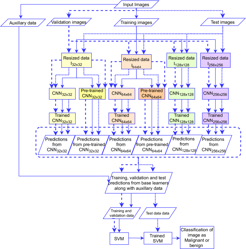
The proposed technique is an ensemble-based technique in which CNNs are used as base learners. The base learners are either pre-trained on balanced dataset collected from ISIC archive or on the the ISIC 2020 dataset. Predictions from all the base learners along with the auxiliary data contained in the metadata associated to the images are used as input to an SVM classifier, which finally classifies each image in dataset as positive (malignant) or negative (benign). Figure 1 shows the flowchart of the proposed technique.

2.1 Architecture

In the proposed technique, six base-learners are used. Each of the base learners operates on input data of different dimensions. During training four base learners, $\mathrm{CNN}_{32\times 32}$, $\mathrm{CNN}_{64\times 64}$, $\mathrm{CNN}_{128\times 128}$, and $\mathrm{CNN}_{256\times 256}$, are trained from random initial parameters on $32\times 32$, $64\times 64$, $128\times 128$, and $256\times 256$ input images respectively. Another two base learners are trained on malignant and benign skin cancer images of sizes $32\times 32$ and $64\times 64$ respectively, which are not part of ISIC 2020 dataset. After training of all six base-learners, predictions from all of them, along with the metadata is then fed into an SVM classifier that functions as the meta classifier. The SVM is trained on the training data and used to finally classify each of the test images as malignant or benign. For both the base and the meta classifiers, the validation data is used to adjust hyperparameters as explained in more detail below.

Figure 1: Block diagram of the proposed technique

2.2 Transfer learning during training of the base-learners

Transfer learning is used to transfer the knowledge extracted from one type of machine learning problem to another [Torrey & Shavlik, 2010, Pan & Yang, 2009]. The domain from where information is extracted is known as the source domain, and the domain where extracted information is applied is called the target domain. The benefit of transfer learning is that it not only saves time that is needed to train the network from scratch but also aid in improving the performance in the target domain.

In the proposed technique, idea of transfer learning is exploited during the training phase of base-learners. We pre-train some of the CNN base-learners on a balanced dataset available on Kaggle collected from the ISIC archive is used. This archive dataset was constructed in 2019, so none of the ISIC 2020 data are included in it. The rest of the base-learners are trained on the ISIC 2020 dataset that comprises the target domain. The introduction of the CNNs pre-trained on balanced data provides a diverse set of predictions, complementing the information coming from the base-learners trained on the ISIC 2020 data. Moreover, since the pre-trained base-learners need to be trained only once instead of re-training them every time we repeat the experiment on random subsets of the ISIC 2020 data (see Sec. 3.2 below), the pre-training saves time.

3 Data and Evaluation Metrics

We use the ISIC 2020 Challenge dataset to train and test the proposed method along with a number of benchmark methods and evaluated their performance with commonly used metrics designed for imbalanced data.

3.1 Dataset and pre-processing

The dataset used in the proposed technique contain 33126 dermoscopic images collected from 2056 patients [Rotemberg et al., 2021]. All the images are labelled using histopathology and expert opinion either as benign or malignant skin lesions. The ISIC 2020 dataset also contains another 10982 test data images without the actual labels, but since we are studying the supervised classification task, we use the labeled data only. All the images are in JPG format of varying dimensions and shape. We use different input dimensions for different base-learners, so we scale the input images to sizes $32\times 32$, $64\times 64$, $128\times 128,$ and $256\times 256$ pixels.

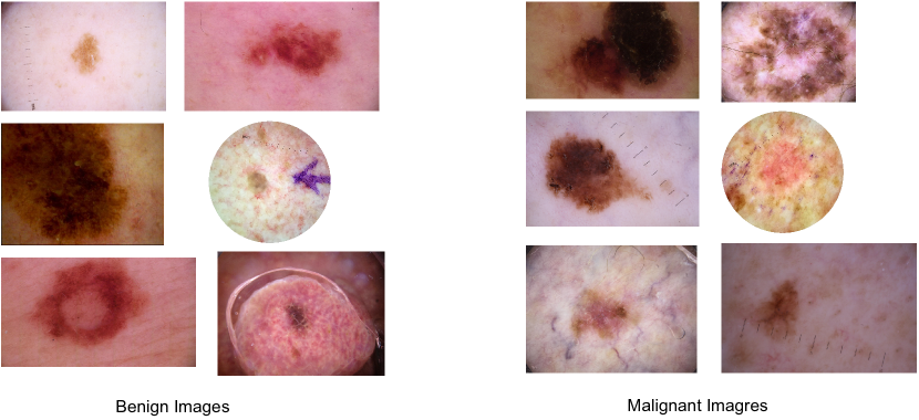
Figure 2 contains example images present in the dataset. Table 1 shows the features in the metadata. Categorical features were encoded as integers in order to reduce the number of parameters in the meta-learner. All the missing values in the metadata are replaced by the average value of the feature in question.

The ISIC 2020 data set is highly imbalanced because out of the total 33126 images (2056 patients), only 584 images (corresponding to 428 distinct patients) are malignant. The division of the data into training, validation, and test sets is described below in Sec 3.2.

Figure 2: Benign vs malignant images

Table 1: Metadata

Variable	Summary
age	min: $10$, max: $90$, median: $50$
sex	female: 48.2 %, male: 51.6%, other/unknown: 0.2 %
general anatomic site	[head/neck, upper extremity, lower extremity,torso, palms/soles, oral/genital]

3.2 Division of the data and hyperparameter tuning

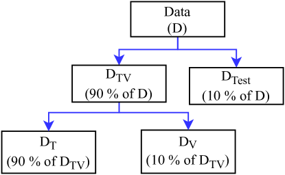
We use the validation set method to divide the data in three parts. As illustrated in Fig. 3, 10 % of the total data $D$ is kept as test data, $D_{\mathrm{Test}}$, which is not used in the training process. The other $90~{}\%$ is further split by using 90 % of it as training data, $D_{\mathrm{T}}$, and the final part as validation data, $D_{\mathrm{V}}$ which is used to tune the hyperparameters of each of the used methods. Since the ISIC 2020 dataset contains multiple images for the same patient, we require that input images from a given individual appear only in one part of the data ($D_{\mathrm{T}}$, $D_{\mathrm{V}}$, or $D_{\mathrm{Test}}$). The validation data is used to adjust the hyperparameters in each of the methods in the experiments by maximizing the F1-score (see Sec. 3.3 below). Hyperparameter tuning was done manually starting from the settings proposed by the original authors (when available) in case of the compared methods, and adjusting them until no further improvement was observed. Likewise, the neural network architectures of the CNN base-learners used in the proposed method were selected based on the same procedure as the other hyperparameters. Tables A1–A6 in the Appendix show the details of the architectures of the CNN base-learners as well as the hyperparameters of the SVM meta-learner.

Figure 3: Division of the data in training, $D_{\mathrm{T}}$, validation $D_{\mathrm{V}}$, and test $D_{\mathrm{Test}}$ sets.

We used the training and validation data from one random train-validation-test split to tune all hyperparameters. We then used the obtained settings in 10 new random repetitions with independent splits to evaluate the classification performance in order to avoid bias caused by overfitting.

3.3 Evaluation metrics

As is customary in clinical applications with imbalanced datasets, we use the F1-measure, the area under the ROC curve (AUC-ROC), and the area under the precision–recall curve (AUC-PR) as evaluation metrics; see, e.g.,  [He & Garcia, 2009]. The F1-measure is the harmonic mean of precision and recall (see definitions below), which is intended to balance the risk of false positives and false negatives. To evaluate the optimal F1-value, we set in each case the classification threshold to the value that maximizes the F1-measure.

AUC-ROC and AUC-PR both characterize the behavior of the classifier over all possible values of the classification threshold. AUC-ROC is the area under the curve between the true positive rate (TPR) and the false positive rate (FPR) at different values of the classification threshold, whereas AUC-PR is the area under the precision–recall curve. While both measures are commonly used in clinical applications, according to Davis & Goadrich [2006] and Saito & Rehmsmeier [2015], AUC-PR is the preferred metric in cases with imbalanced data where false negatives are of particular concern.

The used metrics are defined as follows:

$$\mbox{Precision}=\frac{T_{p}}{T_{p}+F_{p}}$$ (1)

$$\mbox{Recall}=\mathrm{TPR}=\frac{T_{p}}{P}$$ (2)

$$\mathrm{FPR}=\frac{F_{p}}{N}$$ (3)

$$\mbox{F1-measure}=2\times\frac{\mbox{Precision}\times\mbox{Recall}}{\mbox{Precision}+\mbox{Recall}},$$ (4)

where $T_{P}$ is the number of true positives (positive samples that are correctly classified by the classifier), $F_{P}$ is number of false positives (negative samples incorrectly classified as positive), and $P$ and $N$ are the the total number positive and negative samples, respectively.

4 Experimental Results

All the computations were done on the Puhti supercomputer Atlos BullSequana X400 cluster comprised of Intel CPUs. For implementation of the deep learning models we use the Keras version 2.2.4 and TensorFlow version 1.14.0. The other machine learning methods and preprocessing methods were implemented in Python 3.0 and scikit-learn version 0.15.2. All the source code needed to replicate the experiments will be released together with the published version of this paper.

4.1 Main experimental results

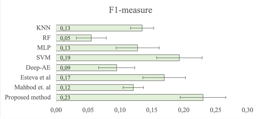
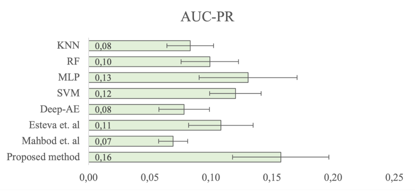
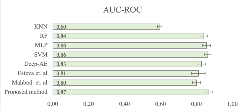
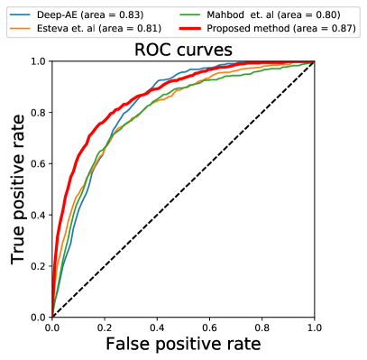
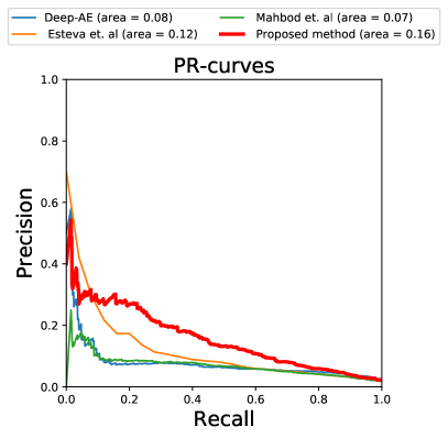
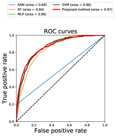
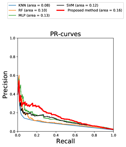
Table 2 and Figure 4 show a comparison of the proposed technique with four non-deep learning classifiers (KNN, RF, MLP, SVM) and three selected deep learning based techniques; see Appendix B for the most important parameters of the benchmark methods. In each of the benchmark methods except those by Esteva et al. [2017] and Mahbod et al. [2019], the $32\times 32$ pixel RGB input images (altogether 3072 input features) along with the auxiliary information in the metadata (additional 3 input features) were used as the input.

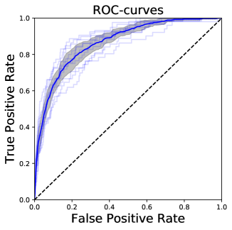
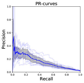
The proposed technique achieves average F1, AUC-PR, and AUC-PR values 0.23, 0.16, and 0.87 respectively, which are highest among all of the compared methods. However, the differences between the top performing methods are within statistical margin of error. A more detailed visualization of the ROC and PR-curves is shown in Figs. 5–7.

Table 2: Comparison of the proposed method with seven other methods in terms of three evaluation metrics (F1-measure, AUC-PR, AUC-ROC). The table shows the average score over $n=10$ random repetitions $\pm$ 95 % confidence intervals based on the $t$-distribution with $n-1=9$ degrees of freedom.

Method	F1-measure	AUC-PR	AUC-ROC
KNN	$0.13\pm 0.02$	$0.08\pm 0.02$	$0.60\pm 0.01$
RF	$0.05\pm 0.02$	$0.10\pm 0.02$	$0.84\pm 0.02$
MLP	$0.13\pm 0.03$	$0.13\pm 0.04$	$0.86\pm 0.02$
SVM	$0.19\pm 0.04$	$0.12\pm 0.02$	$0.86\pm 0.02$
Deep-AE	$0.09\pm 0.03$	$0.08\pm 0.02$	$0.83\pm 0.02$
Esteva et al. [2017]	$0.17\pm 0.03$	$0.12\pm 0.03$	$0.81\pm 0.04$
Mahbod et al. [2019]	$0.12\pm 0.02$	$0.07\pm 0.01$	$0.80\pm 0.02$
Proposed method	$\mathbf{0.23}\pm\mathbf{0.04}$	$\mathbf{0.16}\pm\mathbf{0.04}$	$\mathbf{0.87}\pm\mathbf{0.02}$

Figure 4: Classification accuracy of the proposed method and seven other methods measured by three evaluation metrics (F1-measure, AUC-PR, AUC-ROC). The scores are averages over $n=10$ independent repetitions. Error bars are 95 % confidence intervals based on the $t$-distribution with $n-1=9$ degrees of freedom.

Figure 5: Left: AUC-ROC curves for the proposed method. Right: AUC-PR curves for the proposed method. Both panels show the curves for ten independent runs (light blue curves), the average curve (bold blue line), and an interval showing the standard deviation of the curve (gray region).

Figure 6: Left: Comparison of average ROC curves with three other deep learning methods. Right: Average PR-curves.

Figure 7: Left: Comparison of average ROC with non-deep learning methods. Right: Average PR-curves.

4.2 Performance gain from ensemble learning

The proposed technique in comprised of two steps; in first step base-learners are trained and in second step meta-learner is trained on the top of base-learners. Table 3 shows the performance of each of the base-learners individually, which can be compared with the performance of the resulting SVM meta-classifier that combines the base-learners outputs as the ensemble classification. Out of six base-learners four are trained from scratch on the ISIC 2020 dataset while the remaining two are pre-trained on skin cancer images that are not part of ISIC 2020 dataset. The performance comparison shows that even though the accuracies of each of the base-learners individually are quite low, the meta-classifier performs markedly better. This suggests that the base-learners succeed in providing a diverse set of inputs to the meta-learner, thus significantly improving overall performance of the ensemble over any of the base-learners.

Table 3: Performance of the base-learners and the full ensemble (the SVM meta-classifier), showing the significantly better performance by the ensemble compared to the individual base-learners.

Learner	F1-Measure	AUC-PR	AUC-ROC
$\mathrm{CNN}_{32\times 32}$	$0.09\pm 0.03$	$0.10\pm 0.03$	$0.82\pm 0.04$
$\mathrm{CNN}_{64\times 64}$	$0.12\pm 0.02$	$0.11\pm 0.03$	$0.83\pm 0.02$
$\mathrm{CNN}_{128\times 128}$	$0.13\pm 0.02$	$0.11\pm 0.03$	$0.85\pm 0.02$
$\mathrm{CNN}_{256\times_{2}56}$	$0.11\pm 0.01$	$0.09\pm 0.02$	$0.84\pm 0.04$
pre-trained $\mathrm{CNN}_{32\times 32}$	$0.08\pm 0.01$	$0.04\pm 0.01$	$0.72\pm 0.03$
pre-trained $\mathrm{CNN}_{64\times 64}$	$0.07\pm 0.01$	$0.03\pm 0.01$	$0.71\pm 0.03$
ensemble (SVM meta-classifier)	0.23$\pm$0.04	0.16$\pm$0.04	0.87$\pm$0.02

4.3 Significance of transfer learning and meta-data

To evaluate the impact of the using pre-trained models and that of the metadata on the classification accuracy in the proposed method, we also evaluated the performance with either one of these components disabled. Table 4 shows the performance comparison of the proposed technique to a version where the pre-trained CNNs are disabled, and one where the metadata is not included as auxiliary data for the meta-learner. As seen in the table, excluding the pre-trained CNNs doesn’t significantly affect the performance. The exclusion of the metadata led to somewhat inferior performance, but here too, the differences are relatively minor and with within statistical margin of error. Further research with larger datasets and richer metadata is needed to confirm the benefits.

Table 4: Performance comparison of the proposed technique without pre-trained base-learners and meta-data

Method	F1-measure	AUC-PR	AUC-ROC
without pre-trained base-learners	$\mathbf{0.23}\pm\mathbf{0.04}$	$0.14\pm 0.03$	$\mathbf{0.87}\pm\mathbf{0.02}$
without meta-data	$0.17\pm 0.03$	$0.13\pm 0.04$	$0.86\pm 0.02$
with both (= proposed method)	$\mathbf{0.23}\pm\mathbf{0.04}$	$\mathbf{0.16}\pm\mathbf{0.04}$	$\mathbf{0.87}\pm\mathbf{0.02}$

5 Conclusions

We proposed an ensemble-based deep learning approach for skin cancer detection based on dermoscopic images. Our method uses an ensemble of convolutional neural networks (CNNs) trained of input images of different sizes along with metadata. We present results on the ISIC 2020 dataset which is contains 33126 dermoscopic images from 2056 patients. The dataset is highly imbalanced with less than 2 % of malignant samples. The impact of ensemble learning was found to be significant, while the impact of transfer learning and the use of auxiliary information in the form of metadata associated with the input images appeared to be minor. The proposed method compared favourably against other machine learning based techniques including three deep learning based techniques, making it a promising approach for skin cancer detection especially on imbalanced datasets. Our research expands the evidence suggesting that deep learning techniques offer useful tools in dermatology and other medical applications.

Appendix A: Neural Network Architectures and Hyperparameters of the Proposed Method

Table A1: Parameter setting of $\mathrm{CNN}_{32\times 32}$

Layer	Layer	Kernel size	Feature maps and neurons	Stride	Activation function
0	Input	—	$3\times 32\times 32$	—	Relu
1	Convolutional	$2\times 2$	$64\times 32\times 32$	[1 ,1]	Relu
2	Max pooling	—	$64\times 16\times 16$	[2 ,2]	—
3	Dropout	—	$64\times 16\times 16$	—	—
4	Convolutional	$3\times 3$	$40\times 16\times 16$	[1 ,1]	Relu
5	Max Pooling	—	$40\times 8\times 8$	[2 ,2]	—
6	Convolutional	$3\times 3$	$30\times 8\times 8$	[1 ,1]	Relu
7	Max pooling	—	$30\times 4\times 4$	[2 ,2]	—
8	Convolutional	$3\times 3$	$25\times 4\times 4$	[1 ,1]	Relu
9	Max Pooling	—	$25\times 2\times 2$	[2 ,2]	—
10	Fully connected	—	512	—	Sigmoid
11	Dropout	—	512	—	—
12	Fully connected	—	1	—	Sigmoid

Table A2: Parameter setting of $\mathrm{CNN}_{64\times 64}$

Layer	Layer	Kernel size	Feature maps and neurons	Stride	Activation function
0	Input	—	$3\times 64\times 64$	—	—
1	Convolutional	$2\times 2$	$128\times 64\times 64$	[1 ,1]	Relu
2	Max pooling	—	$128\times 32\times 32$	[2 ,2]	—
3	Dropout	—	$128\times 32\times 32$	—	—
4	Convolutional	$3\times 3$	$80\times 32\times 32$	[1 ,1]	Relu
5	Max Pooling	—	$80\times 16\times 16$	[2 ,2]	—
6	Convolutional	$3\times 3$	$60\times 16\times 16$	[1 ,1]	Relu
7	Max pooling	—	$60\times 8\times 8$	[2 ,2]	—
8	Convolutional	$3\times 3$	$50\times 8\times 8$	[1 ,1]	Relu
9	Max Pooling	—	$50\times 4\times 4$	[2 ,2]	—
10	Fully connected	—	512	—	Sigmoid
11	Dropout	—	512	—	—
12	Fully connected	—	1	—	Sigmoid

Table A3: Parameter setting of $\mathrm{CNN}_{128\times 128}$

Layer	Type of layer	Kernel size	No of feature maps and neurons	Stride	Activation function
0	Input	—	$3\times 128\times 128$	—	—
1	Convolutional	$1\times 1$	$192\times 128\times 128$	[1 ,1]	Relu
2	Max pooling	—	$192\times 64\times 64$	[2 ,2]	—
3	Dropout	—	$192\times 64\times 64$	—	—
4	Convolutional	$3\times 3$	$120\times 64\times 64$	[1 ,1]	Relu
5	Max Pooling	—	$120\times 32\times 32$	[2 ,2]	—
6	Convolutional	$3\times 3$	$90\times 32\times 32$	[1 ,1]	Relu
7	Max pooling	—	$90\times 16\times 16$	[2 ,2]	—
8	Convolutional	$3\times 3$	$75\times 16\times 16$	[1 ,1]	Relu
9	Max Pooling	—	$75\times 8\times 8$	[2 ,2]	—
10	Fully connected	—	512	—	Sigmoid
11	Dropout	—	512	—	—
12	Fully connected	—	1	—	Sigmoid

Table A4: Parameter setting of $\mathrm{CNN}_{256\times 256}$

Layer	Type of layer	Kernel size	No of feature maps and neurons	Stride	Activation function
0	Input	—	$3\times 256\times 256$	—	—
1	Convolutional	$2\times 2$	$256\times 256\times 256$	[1 ,1]	Relu
2	Max pooling	—	$256\times 128\times 128$	[2 ,2]	—
3	Dropout	—	$256\times 128\times 128$	—	—
4	Convolutional	$3\times 3$	$160\times 128\times 128$	[1 ,1]	Relu
5	Max Pooling	—	$160\times 64\times 64$	[2 ,2]	—
6	Convolutional	$3\times 3$	$120\times 64\times 64$	[1 ,1]	Relu
7	Max pooling	—	$120\times 32\times 32$	[2 ,2]	—
8	Convolutional	$3\times 3$	$100\times 32\times 32$	[1 ,1]	Relu
9	Max Pooling	—	$100\times 16\times 16$	[2 ,2]	—
10	Fully connected	—	512	—	Sigmoid
11	Dropout	—	512	—	—
12	Fully connected	—	100	—	Sigmoid
13	Fully connected	—	1	—	Sigmoid

Table A5: Parameter setting of pre-trained $\mathrm{CNN}_{32\times 32}$

Layer	Type of layer	Kernel size	No of feature maps and neurons	Stride	Activation function
0	Input	—	$3\times 32\times 32$	—	Relu
1	Convolutional	$2\times 2$	$200\times 32\times 32$	[1 ,1]	Relu
2	Max pooling	—	$200\times 16\times 16$	[2 ,2]	—
3	Dropout	—	$200\times 16\times 16$	—	—
4	Convolutional	$3\times 3$	$80\times 16\times 16$	[1 ,1]	Relu
5	Max Pooling	—	$80\times 8\times 8$	[2 ,2]	—
6	Convolutional	$3\times 3$	$60\times 8\times 8$	[1 ,1]	Relu
7	Max pooling	—	$60\times 4\times 4$	[2 ,2]	—
8	Convolutional	$3\times 3$	$50\times 4\times 4$	[1 ,1]	Relu
9	Max Pooling	—	$50\times 2\times 2$	[2 ,2]	—
10	Fully connected	—	1024	—	Sigmoid
11	Dropout	—	1024	—	—
12	Fully connected	—	1	—	Sigmoid

Table A6: Parameter setting of pre-trained $\mathrm{CNN}_{64\times 64}$

Layer	Type of layer	Kernel size	No of feature maps and neurons	Stride	Activation function
0	Input	—	$3\times 64\times 64$	—	Relu
1	Convolutional	$2\times 2$	$128\times 64\times 64$	[1 ,1]	Relu
2	Max pooling	—	$128\times 32\times 32$	[2 ,2]	—
3	Dropout	—	$128\times 32\times 32$	—	—
4	Convolutional	$2\times 2$	$80\times 32\times 32$	[1 ,1]	Relu
5	Max Pooling	—	$80\times 16\times 16$	[2 ,2]	—
6	Convolutional	$2\times 2$	$100\times 16\times 16$	[1 ,1]	Relu
7	Max pooling	—	$100\times 8\times 8$	[2 ,2]	—
8	Convolutional	$2\times 2$	$70\times 8\times 8$	[1 ,1]	Relu
9	Max Pooling	—	$70\times 4\times 4$	[2 ,2]	—
10	Fully connected	—	700	—	Sigmoid
11	Dropout	—	700	—	—
12	Fully connected	—	1	—	Sigmoid

Table A7: Parameters of the meta-learner (Support Vector Machine)

Kernel	Degree	$C$	$\gamma$
rbf	2	0.02	0.0009

Appendix B: Hyperparameters of the Compared Methods

We used the following hyperparameters for the compared methods, which were selected manually by adjusting them until no further improvement on the validation data performance (F1-measure) was observed. For the KNN classifier, we use $k=4$. For the random forest (RF), maximum depth 30 and $n=100$ trees are used. For the multilayer perceptron (MLP), we use one hidden layer with 120 neurons, and minibatch size 250. For the support vector machine (SVM), a polynomial kernel of degree 3, and constants $C=0.07$ and $\gamma=0.0009$ are used. In the deep autoencoder (deep-AE), we use an encoder with two layers having 2000 and 1000 neurons, respectively, and a symmetric decoder, and train the model for 100 epochs with minibatch size 15.

References

- Armstrong & Kricker [1995] Armstrong, B. K., & Kricker, A. (1995). Skin cancer. Dermatologic Clinics, 13, 583–594. doi:10.1016/S0733-8635(18)30064-0.
- Ballerini et al. [2013] Ballerini, L., Fisher, R. B., Aldridge, B., & Rees, J. (2013). A color and texture based hierarchical k-nn approach to the classification of non-melanoma skin lesions. In Color Medical Image Analysis (pp. 63–86). Springer. doi:10.1007/978-94-007-5389-1_4.
- Berrar & Lozano [2013] Berrar, D., & Lozano, J. A. (2013). Significance tests or confidence intervals: which are preferable for the comparison of classifiers? Journal of Experimental & Theoretical Artificial Intelligence, 25, 189–206. doi:10.1080/0952813X.2012.680252.
- Bray et al. [2018] Bray, F., Ferlay, J., Soerjomataram, I., Siegel, R. L., Torre, L. A., & Jemal, A. (2018). Global cancer statistics 2018: Globocan estimates of incidence and mortality worldwide for 36 cancers in 185 countries. CA: A Cancer Journal for Clinicians, 68, 394–424. doi:10.3322/caac.21609.
- Buster et al. [2012] Buster, K. J., Stevens, E. I., & Elmets, C. A. (2012). Dermatologic health disparities. Dermatologic Clinics, 30, 53–viii. doi:10.1016/j.det.2011.08.002.
- Chan et al. [2020] Chan, S., Reddy, V., Myers, B., Thibodeaux, Q., Brownstone, N., & Liao, W. (2020). Machine learning in dermatology: current applications, opportunities, and limitations. Dermatology and Therapy, 10, 365–386. doi:10.1007/s13555-020-00372-0.
- Davis & Goadrich [2006] Davis, J., & Goadrich, M. (2006). The relationship between precision-recall and roc curves. In Proceedings of the 23rd International Conference on Machine Learning (pp. 233–240). doi:10.1145/1143844.1143874.
- Dietterich et al. [2002] Dietterich, T. G. et al. (2002). Ensemble learning. The Handbook of Brain Theory and Neural Networks, 2, 110–125.
- Dorj et al. [2018] Dorj, U.-O., Lee, K.-K., Choi, J.-Y., & Lee, M. (2018). The skin cancer classification using deep convolutional neural network. Multimedia Tools and Applications, 77, 9909–9924. doi:10.1007/s11042-018-5714-1.
- Esteva et al. [2017] Esteva, A., Kuprel, B., Novoa, R. A., Ko, J., Swetter, S. M., Blau, H. M., & Thrun, S. (2017). Dermatologist-level classification of skin cancer with deep neural networks. Nature, 542, 115–118. doi:10.1038/nature21056.
- Guo & Yang [2018] Guo, S., & Yang, Z. (2018). Multi-channel-resnet: An integration framework towards skin lesion analysis. Informatics in Medicine Unlocked, 12, 67–74. doi:10.1016/j.imu.2018.06.006.
- He & Garcia [2009] He, H., & Garcia, E. (2009). Learning from imbalanced data. IEEE Transactions on Knowledge and Data Engineering, 21, 1263–1284. doi:10.1109/TKDE.2008.239.
- He et al. [2016] He, K., Zhang, X., Ren, S., & Sun, J. (2016). Deep residual learning for image recognition. In Proceedings of the IEEE Conference on Computer Vision and Pattern Recognition (pp. 770–778). doi:10.1109/cvpr.2016.90.
- Hirano et al. [2020] Hirano, G., Nemoto, M., Kimura, Y., Kiyohara, Y., Koga, H., Yamazaki, N., Christensen, G., Ingvar, C., Nielsen, K., Nakamura, A. et al. (2020). Automatic diagnosis of melanoma using hyperspectral data and googlenet. Skin Research and Technology, 26, 891–897. doi:10.1111/srt.12891.
- Hosny et al. [2020] Hosny, K. M., Kassem, M. A., & Fouad, M. M. (2020). Classification of skin lesions into seven classes using transfer learning with AlexNet. Journal of Digital Imaging, 33, 1325–1334. doi:10.1007/s10278-020-00371-9.
- Kassem et al. [2020] Kassem, M. A., Hosny, K. M., & Fouad, M. M. (2020). Skin lesions classification into eight classes for isic 2019 using deep convolutional neural network and transfer learning. IEEE Access, 8, 114822–114832. doi:10.1109/access.2020.3003890.
- Krizhevsky et al. [2012] Krizhevsky, A., Sutskever, I., & Hinton, G. E. (2012). Imagenet classification with deep convolutional neural networks. In F. Pereira, C. J. C. Burges, L. Bottou, & K. Q. Weinberger (Eds.), Advances in Neural Information Processing Systems (pp. 1097–1105). volume 25.
- Lau & Al-Jumaily [2009] Lau, H. T., & Al-Jumaily, A. (2009). Automatically early detection of skin cancer: Study based on neural netwok classification. In 2009 International Conference of Soft Computing and Pattern Recognition (pp. 375–380). IEEE. doi:10.1109/socpar.2009.80.
- Li & Shen [2018] Li, Y., & Shen, L. (2018). Skin lesion analysis towards melanoma detection using deep learning network. Sensors, 18, 556. doi:10.3390/s18020556.
- Mahbod et al. [2019] Mahbod, A., Schaefer, G., Wang, C., Ecker, R., & Ellinge, I. (2019). Skin lesion classification using hybrid deep neural networks. In ICASSP 2019-2019 IEEE International Conference on Acoustics, Speech and Signal Processing (ICASSP) (pp. 1229–1233). IEEE. doi:10.1109/icassp.2019.8683352.
- Morton & Mackie [1998] Morton, C., & Mackie, R. (1998). Clinical accuracy of the diagnosis of cutaneous malignant melanoma. British Journal of Dermatology, 138, 283–287. doi:10.1046/j.1365-2133.1998.02075.x.
- Murugan et al. [2019] Murugan, A., Nair, S. A. H., & Kumar, K. S. (2019). Detection of skin cancer using svm, random forest and knn classifiers. Journal of Medical Systems, 43, 1–9. doi:10.1007/s10916-019-1400-8.
- Pan & Yang [2009] Pan, S. J., & Yang, Q. (2009). A survey on transfer learning. IEEE Transactions on Knowledge and Data Engineering, 22, 1345–1359. doi:10.1109/tkde.2009.191.
- Pedregosa et al. [2011] Pedregosa, F., Varoquaux, G., Gramfort, A., Michel, V., Thirion, B., Grisel, O., Blondel, M., Prettenhofer, P., Weiss, R., Dubourg, V., Vanderplas, J., Passos, A., Cournapeau, D., Brucher, M., Perrot, M., & Duchesnay, E. (2011). Scikit-learn: Machine learning in Python. Journal of Machine Learning Research, 12, 2825–2830.
- Polikar [2012] Polikar, R. (2012). Ensemble learning. In Ensemble Machine Learning (pp. 1–34). Springer. doi:10.1007/978-1-4419-9326-7_1.
- Rotemberg et al. [2021] Rotemberg, V., Kurtansky, N., Betz-Stablein, B., Caffery, L., Chousakos, E., Codella, N., Combalia, M., Dusza, S., Guitera, P., Gutman, D. et al. (2021). A patient-centric dataset of images and metadata for identifying melanomas using clinical context. Scientific Data, 8, 1–8. doi:10.1038/s41597-021-00815-z.
- Saito & Rehmsmeier [2015] Saito, T., & Rehmsmeier, M. (2015). The precision-recall plot is more informative than the ROC plot when evaluating binary classifiers on imbalanced datasets. PLoS ONE, 10, e0118432. doi:10.1371/journal.pone.0118432.
- Simões et al. [2015] Simões, M. F., Sousa, J. S., & Pais, A. C. (2015). Skin cancer and new treatment perspectives: A review. Cancer Letters, 357, 8–42. doi:10.1016/j.canlet.2014.11.001.
- Simonyan & Zisserman [2015] Simonyan, K., & Zisserman, A. (2015). Very deep convolutional networks for large-scale image recognition. In Y. Bengio, & Y. LeCun (Eds.), 3rd International Conference on Learning Representations (ICLR) 2015.
- Szegedy et al. [2015] Szegedy, C., Liu, W., Jia, Y., Sermanet, P., Reed, S., Anguelov, D., Erhan, D., Vanhoucke, V., & Rabinovich, A. (2015). Going deeper with convolutions. In Proceedings of the IEEE Conference on Computer Vision and Pattern Recognition (pp. 1–9). doi:10.1109/cvpr.2015.7298594.
- Szegedy et al. [2016] Szegedy, C., Vanhoucke, V., Ioffe, S., Shlens, J., & Wojna, Z. (2016). Rethinking the inception architecture for computer vision. In 2016 IEEE Conference on Computer Vision and Pattern Recognition, CVPR 2016 (pp. 2818–2826). IEEE Computer Society. doi:10.1109/CVPR.2016.308.
- Thomas et al. [2021] Thomas, S. M., Lefevre, J. G., Baxter, G., & Hamilton, N. A. (2021). Interpretable deep learning systems for multi-class segmentation and classification of non-melanoma skin cancer. Medical Image Analysis, 68, 101915. doi:10.1016/j.media.2020.101915.
- Torrey & Shavlik [2010] Torrey, L., & Shavlik, J. (2010). Transfer learning. In Handbook of Research on Machine Learning Applications and Trends: Algorithms, Methods, and Techniques (pp. 242–264). IGI global. doi:10.4018/978-1-60566-766-9.ch011.