Understanding performance variability in standard and pipelined parallel Krylov solvers
Abstract
In this work, we collect data from runs of Krylov subspace methods and pipelined Krylov algorithms in an effort to understand and model the impact of machine noise and other sources of variability on performance. We find large variability of Krylov iterations between compute nodes for standard methods that is reduced in pipelined algorithms, directly supporting conjecture, as well as large variation between statistical distributions of runtimes across iterations. Based on these results, we improve upon a previously introduced nondeterministic performance model by allowing iterations to fluctuate over time. We present our data from runs of various Krylov algorithms across multiple platforms as well as our updated non-stationary model that provides good agreement with observations. We also suggest how it can be used as a predictive tool.
1 Introduction
Coherent performance models are important to describe and evaluate algorithms on modern architectures. With good models, HPC users can pick the appropriate method and algorithmic parameters for their application to run in a complicated computing environment. Futhermore, models are important in evaluating HPC systems and moving forward with new architecture and algorithm design.
The increasing complexity of computing environments has introduced many sources of run-to-run variability at different levels of HPC systems. For example, an operating system can interrupt processors at any time for its activities, causing detours in computations and degrading performance ([1, 2]). Inter-job contention for shared resources such as network bandwidth, routers, and links is another source of variability that can affect application performance ([3, 4]). Developing coherent performance models in the presence of variability is difficult ([5, 6]), particularly between systems.
In this work, we advocate for casting performance models in a nondeterministic paradigm that more accurately reflects algorithm execution in noisy HPC environments. Employing stochastic performance models for algorithms that run on HPC systems could reflect a more realistic computing scenario since many detours and sources of variability are unpredictable. Some work has been done using stochastic models to predict performance in HPC environments. For example, [7] studied the impact of different noise distributions on a single collective operation and [8] modeled operating system “jitter" as random variables in order to compute computational slowdown in the presence of noise.
We are interested in modeling standard Krylov subspace methods ([9, 10]) and pipelined variants often used in large-scale simulations to solve sparse systems of equations. Highly synchronous applications such as those that use Krylov subspace methods are vulnerable to performance degradation induced by variability at different machine levels. Because each iteration is performed in lockstep, an operating system interrupt (or any other source of slowdown) that delays a single processor can cause others to be delayed as well. The cost of communication can vary considerably between iterations and runs on modern machines due to network contention or other factors. This can significantly degrade method performance because of the global reduction operations used to compute vector norms and inner products. Motivated by mitigating latency associated with global communication, algebraically equivalent pipelined algorithms of Krylov subspace methods have been introduced ([11, 12, 13, 14, 15, 16]). Pipelined algorithms rearrange computations so that it is possible to hide some of the cost of global communication with local computation, at the cost of increased computation, storage, and degraded numerical stability.
We characterize the performance of standard Krylov subspace methods and pipelined algorithms using experimental data to refine the performance model introduced (see [17]), which used random variables to model iteration times. Such models and data are useful because pipelined Krylov algorithms tend to become more useful in situations where performance data is more difficult to directly gather: with large node counts on congested supercomputers with unpredictable local processing times. We intentionally maintain a data-driven approach, focusing on a simple stochastic model that nevertheless captures a key property of pipelined Krylov algorithms in the context of increasingly-complex computing systems. This is to be strongly contrasted with traditional performance modeling which emphasizes describing best-case scenarios ([18]), attainable speedup, and detailed measurements of presumed-to-be-relevant performance characteristics.
Data is found to directly support the conjecture that pipelined algorithms effectively smooth out variability which in and of itself can give speedup over standard Krylov subspace methods. This demonstrates that in addition to helping to address the scalability bottleneck associated with global reductions, pipelined Krylov algorithms can, by relaxing data dependencies, offer increased performance even when reductions are modeled as simple barriers. This points to these methods being useful in a much wider range of applications, such as those with smaller problem sizes but more variable local times per iteration, or on systems with extremely fast networks that are currently far away from a reduction latency scaling bottleneck.
In this paper, we begin by reviewing the performance models introduced in [17] for Krylov subspace methods and pipelined algorithms in the presence of noise. Next we examine experimental results from runs of these algorithms and refine the performance models based on insights from the data. Specifically, we intend to show the need for non-stationary models. Throughout this work, we use the term “non-stationary” to mean a process (in our case, iterations of a Krylov algorithm) whose probability distribution changes with shifts in time. We employ our stochastic performance models and show that the updated model is in close agreement with reality. Then we present more experimental data and suggest ways to perform a priori performance estimates. Finally, we conclude our work.
2 Stochastic model review
A standard Krylov method is modeled as a set of processes repeatedly performing local computation and global communication. Because of the synchronizations in each of iteration the total time for each iteration is the time given by the slowest processor. Let index the processors and index the iterations. Then, the total time for a Krylov method is modeled as
| (1) |
where is the time for iteration on process . Since this work can be interrupted by operating system noise or other interference, the iteration times might fluctuate over steps and processors. To model this nondeterministic behavior, we let the iterates be random variables and ask for the expected total runtime
| (2) |
If the iterates are identical and independent of processor () and stationary in time (), then we can compute the expected runtime of a Krylov method using the integral expression
| (3) |
where the random variables are drawn from a distribution with probability density function (pdf) and cumulative distribution function (cdf) .
Similarly, we model a pipelined Krylov algorithm as a set of communicating processors. Pipelined algorithms employ split-phase, non-blocking collectives that do not require global synchronizations. Rather, the collective operation is first initialized, say with MPI_Iallreduce(), and later finalized with MPI_Wait() so that useful work can continue between initialization and finalization. Provided no processor falls too far behind, the total time for a pipelined algorithm is the time for the slowest processor to perform all the given work
| (4) |
Because of detours, we do not expect the iteration times to be deterministic. Again, we ask for the expected total run time
| (5) |
letting the iterates be random variables drawn from a distribution. If the iterates are identically distributed with finite mean and variance, independent of process () and stationary in time (), then, in the limit of large , where is the mean of the underlying iteration time distribution with pdf and cdf . So we have an expression to compute the expected total time for a pipelined algorithm
| (6) |
For a more thorough explanation of the arguments presented in this section, see [17]. In the next section we present fine-grained data collected from runs of Krylov methods and pipelined algorithms. This gives us insight into how detours affect these simulations, which assumptions above are realistic, and how the models might be refined.
3 Experimental results
Here we present the results from experiments conducted on the Cray XC40, Theta, at the Argonne Leadership Computing Facility. We choose to run two programs with contrasting characteristics. While this is a limited representation the results are informative. Theta compute nodes each contain a single Xeon Phi Knights Landing (KNL) CPU ([19]) with 64 cores, and are connected by a Cray Aries interconnect in a dragonfly topology ([20]). We use the Portable, Extensible Toolkit for Scientific Computation (PETSc) ([21, 22]) version 3.10 to simulate the solution to problems with varying characteristics such as sparsity pattern. One MPI rank per core is used throughout and we boot the nodes in quadrant clustering mode and flat memory mode, which exposes the on-die, high-bandwidth Multi-Channel DRAM (MCDRAM) as a user-addressable memory, rather than treating it as an L3 cache. We collect iteration times by inserting calls to MPI_Wtime() at the beginning and end of each Krylov cycle in PETSc’s scalable linear equation solvers (KSP) component’s GMRES (generalized minimal residual method) and PGMRES (pipelined GMRES) algorithms ([12]). Since changes and upgrades to HPC machines can affect performance, we note that experiments presented in this paper were performed in autumn 2018 with Cray-MPICH 7.7.3 and built with the Cray C compiler wrapper.
3.1 One-dimensional Laplacian
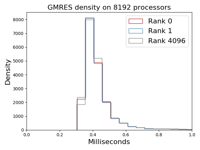
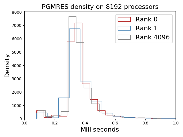
PETSc KSP tutorial ex23111/src/ksp/ksp/examples/tutorials/ex23.c in PETSc 3.10 is a one-dimensional finite-difference discretization of the Laplacian, resulting in a simple tridiagonal system. A simple matrix will subtract the effects of irregular communication in sparse matrix-vector products by removing the need for all but nearest neighbor communication. We show the results from a simulation with a more complicated sparsity pattern in the next section. We run ex23 with GMRES and PGMRES using 8192 MPI processes with unknowns and a Jacobi preconditioner. Throughout these simulations we force 5000 Krylov iterations. We choose to run our experiments with few degrees of freedom per processor since these schemes are often used in this regime and with a large number of iterations to amass statistics.
The stochastic model expressions (3) and (6) place assumptions on the iterates . We check them here to examine the actual performance of the algorithms and to justify use of the models. In Figure 1 we graph the distribution of the iterates for select processors identified by their MPI ranks. The distributions look similar between ranks, implying that the iterations might be identical with respect to process. We make use of the two sample Kolmogorov-Smirnov test to check whether two samples (e.g. iterations from rank 0 and rank 1) are drawn from the same underlying distribution. The Kolmogorov-Smirnov test calculates the distance between the empirical distributions of two samples with empirical distribution functions of size and of size with
| (7) |
We reject the hypothesis that the samples come from the same distribution with significance level if
| (8) |
where is a tabulated value. For GMRES, and for PGMRES. We use significance level and SciPy’s stat.ks_2samp function to calculate the test statistic . We find that we do not reject that GMRES ranks 0 and 1 come from the same distribution with significance level since , the threshold. For PGMRES ranks 0 and 1, , so we reject the null hypothesis. On rank 1, we reject none of the pairs of GMRES ranks and reject of PGMRES pairs.
Because it is inefficient to orthogonalize new Krylov vectors against a large basis, GMRES methods are typically implemented to restart after iterations. When a Krylov subspace method restarts, the basis for the Krylov subspace is discarded and the current solution is used as the initial guess for the next cycle. PETSc implements a pipelined GMRES algorithm given by [12] which adds two iterations in each cycle to "fill the pipeline." Since the PETSc default restart value is , 5334 iterations of PGMRES are actually employed instead of 5000. Some of these are very quick and easily identifiable as the bump of very short iterations in Figure 1 (bottom). Still, we compare 30 GMRES iterations to 32 of PGMRES since they compute the same number of intermediate solutions which are, moreover, the same in exact arithmetic.
Figure 2 shows the time for iterations (GMRES) and (PGMRES), halfway through the Krylov cycle described before, on process in order of MPI rank. We include a inset graph that shows the iterations on the first ten nodes, delineated by black lines. GMRES iterates are nearly constant on a node; each KNL node of 64 processes is clearly visible in Figure 2 (top, inset) so that the iterations are not truly independent in as we assumed above. The variance of iteration times on node 0 (with MPI ranks 0-63) is . This could be due to the synchronizations in each iteration of GMRES that force processes on a node to perform in lockstep. There is also some periodic behavior over all the nodes. Conversely, PGMRES iterations contain more variability on a node ( on the node with MPI ranks 0-63, three orders of magnitude greater than GMRES), but less between them.


Figure 3 is a 2-color colormap of the iterates for all iterations and all processors. Graphed are the iterations that perform the “average" amount of work during each GMRES cycle (GMRES iteration and PGMRES ) so that each iteration shown performs the same computation. Horizontal lines are highly visible, implying that processors perform similarly within a given iteration. The difference between different iterations is also clear; iterate timings fluctuate in time without an obvious pattern. In the absence of an algorithmic reason that some iterations should take longer than others, after taking restarts into account, these differences could be explained by long operating system interruptions, thermal throttling of the CPU, or other external causes. Furthermore, some groups of iterations (GMRES iterations or PGMRES ) overall take longer than other iterations.
3.2 Three-dimensional non-Newtonian fluid
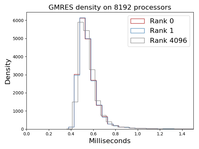
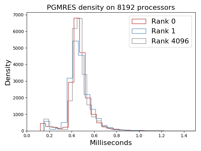
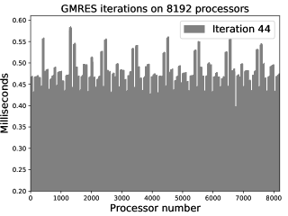
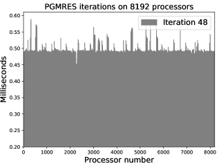
PETSc SNES tutorial ex48222src/snes/examples/tutorials/ex48.c in PETSc 3.10 solves the Blatter-Pattyn hydrostatic equations that model ice sheet flow for glaciers ([23]). For the ice, we use a power-law rheology with Glen exponent 3. This generates a much denser system of equations with about 10 times more nonzeros per row than ex23 and requires extensive communication across the machine, resulting in more network traffic and the possibility for more variable communication latency. Again we choose our problem size so that there are unknowns, use a Jacobi preconditioner, and force 5000 iterates of the Krylov algorithm. We stop after one nonlinear iteration.
We repeat the analysis from before and find qualitatively similar results, shown in Figure 4. Using the Kolmogorov-Smirnov test again we find that we do not reject the assumption that GMRES iterates from ranks 0 and 1 come from the same distribution since and we reject that PGMRES iterates come from the same distribution since . The iterates on a fixed process look like they could be from the same family of distributions with different parameters as those in the previous subsection.
GMRES iterates again appear highly dependent on the node with node 0 variance . The variance on PGMRES node 0 is , larger than before, and there is more variation between PGMRES nodes which looks periodic. This could be explained by the communication induced by the matrix sparsity pattern.
4 Non-stationary performance model
Based on the results from the last section, we move to a non-stationary performance model where the iterates can fluctuate in time. The expected total time for a Krylov method is still given by
but we relax the claim that the iterates are stationary in time. In iteration , the random variables are drawn from a distribution with cdf and pdf , which can now fluctuate across steps. Then the expected runtime of a Krylov method is given by
| (9) |
We call this the “non-stationary" performance model and distinguish between in (3) and here.
Similarly for a pipelined algorithm, we use (5) as before and drop the assumption that the iterates are stationary in time, so that
| (10) |
where is the mean of the underlying distribution in iteration .
The original Krylov model (3) benefits from slight alteration as well. Since the iterates on each node are nearly constant, shown in Figure (2) (left) and Figure 4 (bottom left), they are more suitably modeled by independent random variables than independent processors. We make use of this substitution in the next section but it does not seem to strongly affect (9).
5 Performance modeling
In this section, we will deploy our performance models and test them against collected data.
5.1 Computing expected runtimes
The expressions for and say that the iterates come from some underlying distribution with pdf , cdf , and mean . We will use “bulk statistics" with these performance models, taking all iterations for all processors in aggregate, for the underlying distribution and to characterize the iteration times and machine variation.
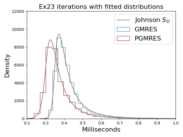
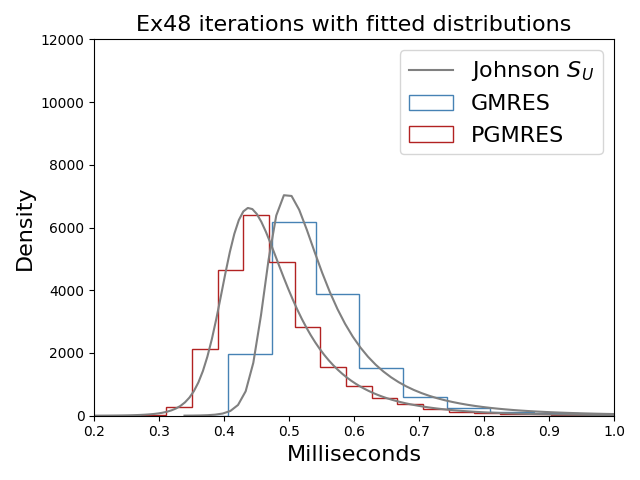


To find the functions and and mean , we use Scipy’s stats package to fit various analytical distributions to our collected data. For a given continuous distribution and data, the fit function returns the maximum likelihood estimation for the shape, location, and scale parameters by maximizing a log-likelihood function. We choose distributions which minimize the sum of squared error between the data and the fit distribution. For the pipelined algorithms, we disregard the two iterations in each cycle that “fill the pipeline" to avoid distribution fitting complications.
Using these well-fitting distributions, we can calculate and and compare the expected results to the KSPSolve time (the time spent inside the Krylov solver) provided by PETSc’s -log_view option. For integration in (3) we use Python’s scipy.integrate.quad function and integrate over the bounds of the data.
To employ the updated models and , we again perform distribution fitting using scipy, this time for each iteration to find , , and mean . GMRES and PGMRES iteration data is shown in Figure 6. It is quite clear that these are far from normal and do not resemble well-known distributions. Because of this, and in the interest of simplicity, we treat runtimes for each iteration as coming from a uniform distribution with possibly different parameters. Again, integration is performed in each iteration again using scipy.integrate.quad and the calculated expected total times are compared to the KSPSolve time.
Analytical expressions have been used to bound the maximum of a set of random variables using the sample mean and standard deviation ([8]). Cramer ([24, 25]) bound the maximum of identical and independent random variables with
| (11) |
and (Bertsimas [26]) bound the maximum of identical, but not independent random variables by
| (12) |
We will use these to compare with our Krylov performance models.
5.2 Results
Distribution fitting alone gives some insight into algorithm execution. In Figure 5, we show bulk data from our experimental results with the Johnson distribution, a transformation of the normal distribution with pdf
| (13) |
with shape paramters and and where is the normal pdf. Note that there were some other well-fitting distributions, including Non-central Student’s T. The bulk data show that in a given method, the iterates are mostly clustered and fairly quick with a fewer, longer, giving the distribution a small tail. In general, PGMRES runtimes were faster than GMRES, consistent with faster overall execution in these examples. Ex48 runtimes are shifted to the right of ex23 and more spread out, implying longer iterations with more variation.
| ex23 | KSPSolve | Cramer bound | Bertsimas bound | |||
|---|---|---|---|---|---|---|
| GMRES | 2.217 | 4.831 | 4.365 | 2.432 | 6.35 | 8.102 |
| PGMRES | 2.006 | 1.865 | 1.868 | 1.857 | ||
| ex48 | ||||||
| GMRES | 2.943 | 5.716 | 10.88 | 3.189 | 20.59 | 27.99 |
| PGMRES | 2.656 | 2.413 | 2.413 | 2.455 |
| Uniform | Uniform | |||||||
|---|---|---|---|---|---|---|---|---|
| ex23 | loc | scale | loc | scale | ||||
| GMRES | -5.86e-01 | 3.35 | 3.97e-04 | 1.07e-21 | -7.40e-01 | 3.21 | 8.06e-04 | 1.86e-23 |
| PGMRES | 2.84 | 6.74 | 3.10e-04 | 2.26e-19 | -6.18e-02 | 2.42 | 2.21e-03 | 6.47e-19 |
| ex48 | ||||||||
| GMRES | 6.74e-01 | 2.09 | 2.22e-02 | 2.24e-24 | 6.69e-01 | 2.10 | 1.71e-03 | 9.23e-26 |
| PGMRES | -6.02e-01 | 3.34 | 4.07e-04 | 3.05e-23 | 1.24 | 1.84 | 1.36e-02 | 1.66e-18 |
Results for the data presented in our experimental results are shown in Table 1 for PETSc ex23 and ex48. It is clear that applying the non-stationary performance model to standard Krylov subspace methods gives a large improvement over the stationary model . The stationary model overestimates actual runtimes and the analytical bounds are very loose and not particularly helpful. Both models are good estimates for pipelined algorithms, suggesting that modeling a method without explicit synchronization is more flexible.
In this work we don’t compare our results to more algorithm-specific models or those that collect detailed hardware measurements, instead emphasizing a paradigm where the use of simple, general models is sufficient to approximate the execution time for Krylov solvers without collecting low-level information.
6 Predicting runtimes
In the previous section, we showed that our performance models and can reasonably predict execution time when we have the time for iteration on process for all and .
While bulk statistics appear to be enough to succinctly describe the performance of a pipelined algorithm, they are not a sufficient way to describe a traditional Krylov method. Instead, we will use non-stationary distributions to model each iteration. GMRES and PGMRES distribution data is shown with uniform distributions in Figure 6. Here we see how much the iterations shift in time. They are mostly non-overlapping. We also want to know how the uniform parameters change over time. That is, for each iteration , the random variables are modeled as following a uniform distribution with pdf and cdf given by
| (14) |
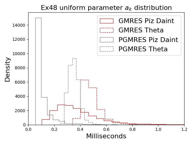
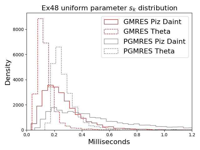
The uniform distribution can be described with two parameters: the minimum and the span . We model a Krylov method with uniform distributions where in each iteration the uniform parameters and are random variables themselves drawn from some distribution. Figure 7 show histograms of the uniform parameters from PETSc ex48 using GMRES and PGMRES with fitted Johnson distribution. This distribution has the pdf (13) and is described by two shape parameters and and location and scale parameters loc and scale in Scipy .
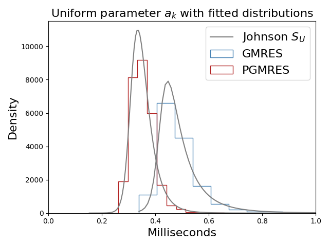
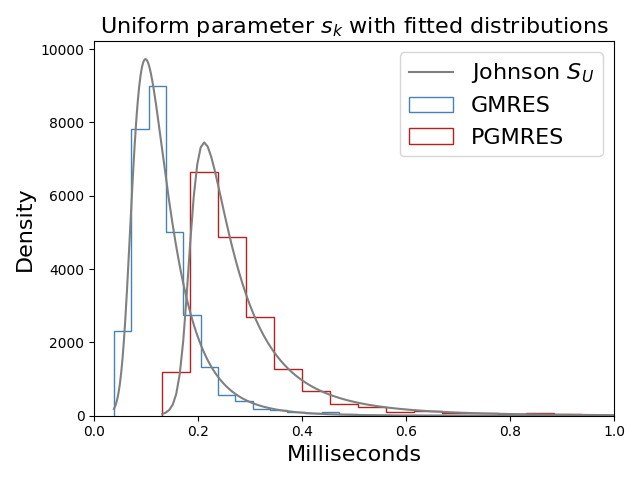
Table 2 shows Johnson parameters for the uniform distribution parameters from Figure 7 and PETSc ex23. In general, they show that, in a given iteration, the fastest processor is generally faster in a PGMRES run, but the runtimes are more spread out. All Johnson distributions are shaped such that they lean left with a tail, some longer than others.
We can mimic a Krylov computation by “simulating” the iterations with a Monte Carlo-type approach. We assume that each iteration time is uniformly distributed with parameters and in iteration
We further assume that the parameters and are themselves random variables drawn from a Johnson distribution with parameters , , loc, and scale.
We draw random variables and using Scipy’s rvs function and compute the expected time for iteration , , given by
| (15) |
Repeating for iterations, we get . We simulate a pipelined Krylov computation in the same way, pulling random variables and and computing
| (16) |
where is the mean of . Table 3 shows the results of this simulation using the Johnson parameters from Table 2. The results are good when we have the computed Johnson parameters. The challenge in general will be to reason about these parameters so that we can make a priori performance estimates for standard Krylov methods and pipelined algorithms.
| ex23 | GMRES | PGMRES | ex48 | GMRES | PGMRES |
|---|---|---|---|---|---|
| KSPSolve | 2.217 | 2.006 | KSPSolve | 2.943 | 2.656 |
| Simulated | 2.416 | 1.908 | Simulated | 3.14 | 2.482 |
7 Extension to other algorithms and computing platforms
In the last section, we saw that we can reasonably estimate the execution time of a Krylov method given that we know the Johnson parameters that model and . Many factors, such as algorithm and matrix pattern, can influence performance. In this section, we expand our experiments to study other factors including problem size and computing platform and test our non-stationary model in more scenarios.
7.1 Scaling experiments
Our experiments so far have been performed on 8192 processors with unknowns. To see how changing processor count and problem size affect the Krylov method performance and underlying uniform parameters, we run strong- and static-scaling experiments. Figures 8 and 9 show the Johnson distributions for the uniform parameters and for strong- and static-scaling experiments on Theta.
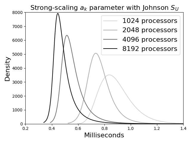
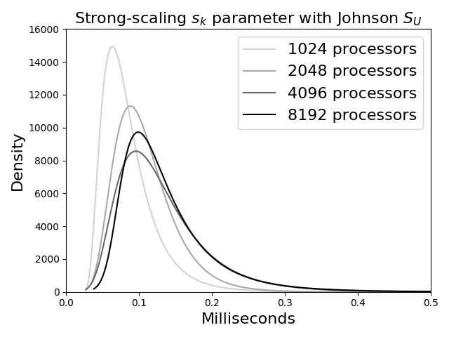
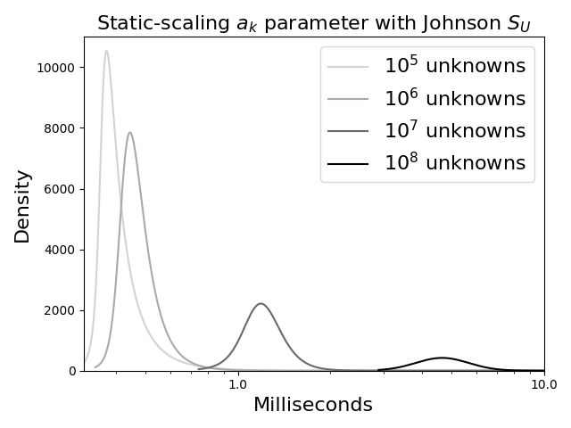
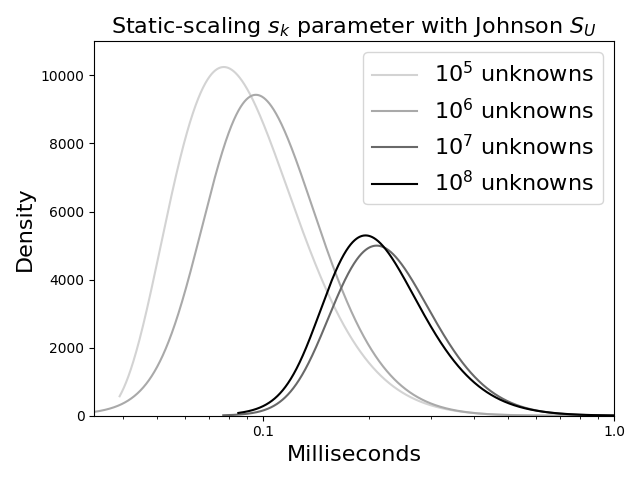
With strong-scaling experiments, we see how varying the processor count affects Krylov method performance for a fixed problem. We repeat runs of ex48 with unknowns on processors. We see that, for a fixed number of unknowns, as we decrease the number of processors the Johnson distribution shifts to the right and spreads out for the uniform parameter. In this case, each processor does more work and is more likely to experience a detour. Similarly, we perform static-scaling experiments. In static-scaling, the problem size (or number of unknowns) is varied on a fixed number of processors. This allows us to see the effect of computation without changing the communication pattern. We keep the number of processors fixed at and vary the number of unknowns, which exaggerates what we see for strong-scaling as shown in Figure 9.
7.2 BiCGSTAB
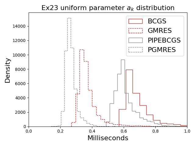
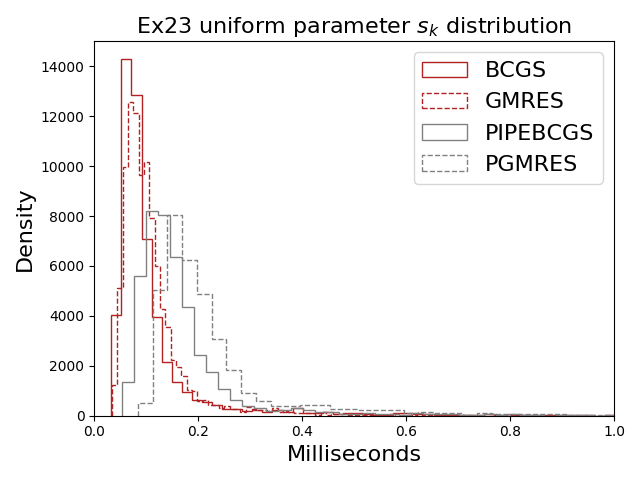
We solve PETSc ex23, the one-dimensional Laplacian problem, using the Stabilized Biconjugate Gradient method (BiCGSTAB) ([27]) and a pipelined version (PIPEBiCGSTAB) ([28]) with 5000 linear iterations and unknowns on Theta. We choose these methods because their communication and performance characteristics differ somewhat from GMRES, as the methods are based on a short-term recurrence relation and do not require orthogonalizing against a growing set of basis vectors; BiCGSTAB and variants also require two matrix-vector multiplications per iterations, instead of one.
Many aspects of the BiCGSTAB and PIPEBiCGSTAB computations are consistent with GMRES and PGMRES, such as non-stationary iterates and nearly constant BiCGSTAB runtimes on a given node of Theta. Figure 10 shows uniform parameter and histograms with GMRES and PGMRES for comparison. It appears that BiCGSTAB and PIPEBiCGSTAB distributions can be modeled by the Johnson distribution family. This suggests that our performance model is applicable to Krylov methods outside of GMRES methods. GMRES and PGMRES outperform BiCGSTAB and PIPEBiCGSTAB and have quicker minimum iteration times ( Johnson distributions shifted to the left for uniform parameter ), but runtimes are tightly grouped. Performance results for BiCGSTAB and PIPEBiCGSTAB using our non-stationary stochastic models are in shown Table 4.
7.3 Piz Daint
We repeat experiments on the Cray XC40 Piz Daint supercomputer333hybrid partition, November 2018, PETSc 3.10, Cray-MPICH 7.7.2 at the Swiss National Computing Center. Piz Daint and Theta both employ a Aries Dragonfly interconnect but Piz Daint contains Intel Xeon E5 Haswell processors ([29]) on compute nodes (which provide more performance per CPU core compared to KNL). Therefore, the differences we see are likely due to different processors or the shared use of a communication network. Figure 11 shows runs of ex48 with GMRES and PGMRES on 8192 processors and unknowns. In a given iteration, the quickest processor can be much faster on Piz Daint than Theta, but both uniform parameters contain much more variation. Non-stationary performance model results from Piz Daint are in shown Table 4.
| Theta | Piz Daint | Mira | |||||
|---|---|---|---|---|---|---|---|
| ex23 | BiCGSTAB | PIPEBiCGSTAB | ex48 | GMRES | PGMRES | GMRES | PGMRES |
| KSPSolve | 3.957 | 3.53 | KSPSolve | 3.029 | 2.642 | 3.026 | 2.804 |
| 4.227 | 3.512 | 3.541 | 2.473 | 3.189 | 2.455 | ||

7.4 Mira
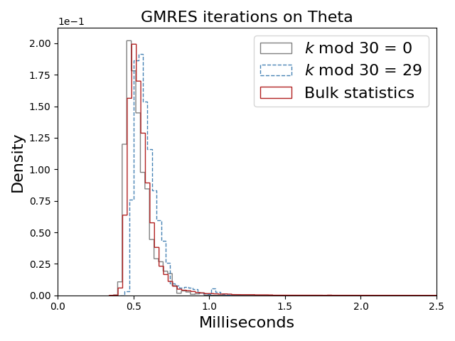
We repeat ex48 experiments on Mira, an IBM Blue Gene/Q444November 2018, PETSc 3.10, MPICH2 1.5 ([30]) at Argonne’s ALCF. We expect a marked performance difference on Mira since nodes on Mira are connected by a 5D torus network with special hardware support for collective communication. Conversely, nodes on Theta are connected by a Cray Aries Network where neighboring workloads share network routes, increasing performance variability ([31]). Each Blue Gene/Q node also contains a redundant processor to service operating system interrupts, similar to Cray’s core specialization feature where one core per node is dedicated to handling OS operations, which reduces core variability ([4]).
Figure 12 shows histograms of iterations from difference places in the GMRES restart cycle as well as a bulk histogram for all iterations from all processors, which can be thought of as the average performance. Each curve has been normalized to represent a distribution. GMRES iterations on Theta at different places in the cycle appear similar to the average. They are noisy enough that our simulation provided reasonable results even though we drew uniform parameters and from the same Johnson distributions regardless of in the GMRES cycle. With Mira’s quiet network, the GMRES iterates are much more distinct suggesting that a refined model that accounts for the amount of work done per iteration would be needed for a priori estimates. Futhermore, we see a jump in the time between iterations and , which is mostly likely due to L1 data cache effects as the required storage for basis vectors increases throughout a GMRES cycle. Similar results were found for PGMRES and performance results are in Table 4.
8 Conclusion and future work
In this work we gather fine-grained iteration data from runs of various Krylov subspace methods across multiple HPC platforms and for different computations. We examine the iterates over time and find that they are non-stationary. That is, the distribution of runtimes shifts with time even after accounting for the growing Krylov subspace. We see significant inter-node variability as well as some intra-node variability, possibly from reduction operations, synchronizations, or operating system interrupts, hindering the performance of traditional Krylov methods. Inhomogeneity from communication patterns is another source of variation between processor performance.
Using these insights, we develop a non-stationary, stochastic performance model that accurately reflects the performance of standard Krylov methods and pipelined algorithms across different algorithms and a variety of HPC architectures. Furthermore, this model suggests a way to make predictive performance estimates.
Future work should conduct experiments on a more comprehensive set of problems, gathering a wider range of runtimes for testing. We also plan to measure different components of Krylov iterations such as communication phases with orthogonalizations and make use of hardware counters. Also in the future, nondeterministic performance models can be derived for other parallel algorithms where unpredictable system interference could impact performance. We also plan on testing our model with heavier preconditioners, deeper pipelines, and more complex architectures. Since we made no assumptions about the hardware in our performance models, we could deploy the same experiments on, for example, a heterogenous machine with GPUs and analyze the data in a similar way.
Accurate performance models can assist in algorithmic choices and parameter tuning such as pipeline depth. Insights from performance models can also be used to guide the development of new algorithms, particularly those we expect to be running in less predictable computing environments, such as heavily loaded machines or loosely coupled networks used in cloud computing or those with shared resources.
Acknowledgements
Thanks to everyone who offered insight and advice, including Todd Munson, Barry Smith, Ivana Marincic, Vivak Patel, Karl Rupp, and Oana Marin.
Funding
The authors were supported by the U.S. Department of Energy, Office of Science, Advanced Scientific Computing Research un- der Contract DE-AC02-06CH11357. This research used resources of the Argonne Leadership Computing Facility, which is a DOE Office of Science User Facility supported under Contract DE-AC02- 06CH11357. The authors were partially supported by the Exascale Computing Project (17-SC-20-SC), a collaborative effort of the U.S. Department of Energy Office of Science and the National Nuclear Security Administration. P. S. acknowledges financial support from the Swiss University Conference and the Swiss Council of Federal Institutes of Technology through the Platform for Advanced Scientific Computing (PASC) program.
References
- [1] Torsten Hoefler, Timo Schneider, and Andrew Lumsdaine. Characterizing the influence of system noise on large-scale applications by simulation. pages 1–11. Proceedings of the International Conference for High Performance Computing, Networking, Storage and Analysis, IEEE/ACM, 2010.
- [2] Kurt B. Ferreira, Patrick Bridges, and Ron Brightwell. Characterizing application sensitivity to OS interference using kernel-level noise injection. pages 19:1–19:12, Piscataway, NJ, 2008. Proceedings of the Conference on Supercomputing, IEEE/ACM.
- [3] Scott Parker, Vitali Morozov, Sudheer Chunduri, Kevin Harms, Chris Knight, and Kalyan Kumaran. Early evaluation of the Cray XC40 Xeon Phi system Theta at Argonne. Cray User Group Proceedings, 2017.
- [4] Sudheer Chunduri, Kevin Harms, Scott Parker, Vitali Morozov, Samuel Oshin, Naveen Cherukuri, and Kalyan Kumaran. Run-to-run variability on Xeon Phi based Cray XC systems. page 52. Proceedings of the International Conference for High Performance Computing, Networking, Storage and Analysis, ACM, 2017.
- [5] Pete Beckman, Kamil Iskra, Kazutomo Yoshii, and Susan Coghlan. The influence of operating systems on the performance of collective operations at extreme scale. pages 1–12. The International Conference on Cluster Computing, IEEE, 2006.
- [6] T. Hoefler, A. Lumsdaine, and W. Rehm. Implementation and performance analysis of non-blocking collective operations for MPI. Proceedings of the International Conference on High Performance Computing, Networking, Storage and Analysis, IEEE/ACM, Nov. 2007.
- [7] Saurabh Agarwal, Rahul Garg, and Nisheeth K Vishnoi. The impact of noise on the scaling of collectives: A theoretical approach. pages 280–289. International Conference on High-Performance Computing, Springer, 2005.
- [8] Seetharami Seelam, Liana Fong, Asser Tantawi, John Lewars, John Divirgilio, and Kevin Gildea. Extreme scale computing: Modeling the impact of system noise in multicore clustered systems. pages 1–12. International Symposium on Parallel & Distributed Processing, IEEE, 2010.
- [9] Yousef Saad. Iterative Methods for Sparse Linear Systems. PWS Publishing Company, Boston, 1996.
- [10] H. van der Vorst. Iterative Krylov methods for large linear systems. Cambridge University Press, 2003.
- [11] A. T. Chronopoulos and C. W. Gear. -Step iterative methods for symmetric linear systems. J Comput Appl Math., 25:153–168, 1989.
- [12] Pieter Ghysels, Thomas J Ashby, Karl Meerbergen, and Wim Vanroose. Hiding global communication latency in the GMRES algorithm on massively parallel machines. SIAM J Sci Comput, 35(1):C48–C71, 2013.
- [13] P. Ghysels and W. Vanroose. Hiding global synchronization latency in the preconditioned conjugate gradient algorithm. Parallel Comput, 40(7):224–238, 2014.
- [14] R. Strzodka and D. Göddeke. Pipelined mixed precision algorithms on FPGAs for fast and accurate PDE solvers from low precision components. pages 259–270. Proceedings of the Symposium on Field-Programmable Custom Computing Machines, IEEE, 2006.
- [15] E. De Sturler and H. A. van der Vorst. Reducing the effect of global communication in GMRES(m) and CG on parallel distributed memory computers. Appl Numer Math, 18:441–459, 1995.
- [16] Thierry Jacques, Laurent Nicolas, and Christian Vollaire. Electromagnetic scattering with the boundary integral method on MIMD systems. Parallel Numerical Computation with Applications, pages 215–230, 1999.
- [17] Hannah Morgan, Matthew G. Knepley, Patrick Sanan, and L. Ridgway Scott. A stochastic performance model for pipelined Krylov methods. Concurr Comput, 28(18):4532–4542, 2016.
- [18] W. Gropp and E. L. Lusk. Reproducible measurements of MPI performance characteristics. Proceedings of the 6th European PVM/MPI Users’ Group Meeting on Recent Advances in Parallel Virtual Machine and Message Passing Interface, pages 11–18, 1999.
- [19] Avinash Sodani. Knights landing (KNL): 2nd generation Intel® Xeon Phi processor. pages 1–24. Hot Chips 27 Symposium, IEEE, 2015.
- [20] Bob Alverson, Edwin Froese, Larry Kaplan, and Duncan Roweth. Cray xc series network. Cray Inc., White Paper WP-Aries01-1112, 2012.
- [21] Satish Balay, Shrirang Abhyankar, Mark F. Adams, Jed Brown, Peter Brune, Kris Buschelman, Lisandro Dalcin, Alp Dener, Victor Eijkhout, William D. Gropp, Dinesh Kaushik, Matthew G. Knepley, Dave A. May, Lois Curfman McInnes, Richard Tran Mills, Todd Munson, Karl Rupp, Patrick Sanan, Barry F. Smith, Stefano Zampini, Hong Zhang, and Hong Zhang. PETSc users manual. Technical Report ANL-95/11 - Revision 3.10, Argonne National Laboratory, 2018.
- [22] Satish Balay, Shrirang Abhyankar, Mark F. Adams, Jed Brown, Peter Brune, Kris Buschelman, Lisandro Dalcin, Alp Dener, Victor Eijkhout, William D. Gropp, Dinesh Kaushik, Matthew G. Knepley, Dave A. May, Lois Curfman McInnes, Richard Tran Mills, Todd Munson, Karl Rupp, Patrick Sanan, Barry F. Smith, Stefano Zampini, Hong Zhang, and Hong Zhang. PETSc Web page, 2018.
- [23] Frank Pattyn, Laura Perichon, Andy Aschwanden, Beate Breuer, Brigitte De Smedt, Olivier Gagliardini, G Hilmar Gudmundsson, Richard Hindmarsh, Alun Hubbard, Jesse V Johnson, et al. Benchmark experiments for higher-order and full Stokes ice sheet models (ISMIP-HOM). The Cryosphere Discussions, 2(1):111–151, 2008.
- [24] Harald Cramér. Mathematical methods of statistics, volume 9. Princeton University Press, 2016.
- [25] Herbert Aron David and Haikady Navada Nagaraja. Order statistics. Encyclopedia of Statistical Sciences, 9, 2004.
- [26] Dimitris Bertsimas, Karthik Natarajan, and Chung-Piaw Teo. Tight bounds on expected order statistics. Probab Eng Inf Sci, 20(4):667–686, 2006.
- [27] Henk A van der Vorst. Bi-CGSTAB: A fast and smoothly converging variant of Bi-CG for the solution of nonsymmetric linear systems. SIAM J Sci Stat Comput, 13(2):631–644, 1992.
- [28] Siegfried Cools and Wim Vanroose. The communication-hiding pipelined BiCGStab method for the parallel solution of large unsymmetric linear systems. Parallel Comput, 65:1–20, 2017.
- [29] Per Hammarlund, Alberto J Martinez, Atiq A Bajwa, David L Hill, Erik Hallnor, Hong Jiang, Martin Dixon, Michael Derr, Mikal Hunsaker, Rajesh Kumar, et al. Haswell: The fourth-generation Intel core processor. IEEE Micro, 34(2):6–20, 2014.
- [30] Kalyan Kumaran. Introduction to Mira. Code for Q Workshop, 2016.
- [31] Taylor Groves, Yizi Gu, and Nicholas J Wright. Understanding performance variability on the Aries dragonfly network. International Conference on Cluster Computing, IEEE, 2017.
The submitted manuscript has been created by UChicago Argonne, LLC, Operator of Argonne National Laboratory (“Argonne”). Argonne, a U.S. Department of Energy Office of Science laboratory, is operated under Contract No. DE-AC02-06CH11357. The U.S. Government retains for itself, and others acting on its behalf, a paid-up nonexclusive, irrevocable worldwide license in said article to reproduce, prepare derivative works, distribute copies to the public, and perform publicly and display publicly, by or on behalf of the Government. The Department of Energy will provide public access to these results of federally sponsored research in accordance with the DOE Public Access Plan. http://energy.gov/downloads/doe-public-accessplan