Inflationary magnetogenesis: solving the strong coupling and its non-Gaussian signatures

Debottam Nandi
Abstract

The simplest model of primordial magnetogenesis can provide scale-invariant magnetic fields that can explain the present abundances of it in the cosmic scales. Two kinds of solutions of the coupling function can lead to such phenomena and both of them suffer from the problems of either strong-coupling or large backreaction. In this work, we consider the coupling function as a linear combination of both kinds with a model parameter. We find that the parameter needs to be as small as 1020similar-toabsentsuperscript1020\sim 10^{-20} in order to evade the backreaction problem. On the other hand, requiring that the modes above Mpc scales do not suffer strong coupling, we also obtain a weak constraint of the model parameter to be greater than 1060superscript106010^{-60}. For the allowed range of the model parameter, we, then, analytically evaluate the cross-correlation functions between the magnetic fields and the curvature perturbation. We find that such a combination preserves the consistency relation. Also, the result leads to enhanced non-Gaussianity in equilateral as well as flattened limits with unique signatures that characterize the novelty of this model.

1 Introduction

Astrophysical observations suggest the abundances of large scale coherent magnetic fields in all cosmic scales. These fields are not only present in bound cosmological structures e.g. stars, galaxies, and the cluster of galaxies but they also seem to be present in the intergalactic medium and large scale structures. In galaxies and clusters of galaxies, the strengths of the magnetic fields have been measured to be a few micro Gauss, they are estimated to be of the order of 1017superscript101710^{-17} Gauss in Mpc length scales in intergalactic medium [1, 2, 3, 4, 5, 6, 7, 8, 9] and large scale structures [10, 11, 12, 13, 14, 15, 16].

The origin of such magnetic fields is still unknown. Various explanations that have been put forward can broadly be classified into two categories: Astrophysical and Primordial [17, 18, 19, 20]. The primary issue with the astrophysical sources is that, they cannot explain the coherent length of the field. It is therefore believed that the magnetic field is generated in the early universe and are then amplified by the galactic dynamo mechanism at late times to give rise to such strength of the fields in those scales.

Inflationary paradigm [21, 22, 23, 24, 25, 26, 27, 28, 29, 30, 31, 32, 33] is currently is the most successful early Universe paradigm that can explain the Cosmic Microwave Background Radiation (CMBR) and the formation of large scale structures. However, during this time, the standard electromagnetic (EM) field decays very fast due to its conformal invariance structure in the four dimensions and thus it can still not generate sufficient seed magnetic fields. Therefore, it has been realized that to generate such strength, the necessary condition is to break the conformal symmetry of the EM field. Several authors have suggested many ways to break the conformal invariance of the EM field by introducing (i) a coupling of the EM field with the Ricci/Riemann tensors, (ii) a non-minimal coupling of the EM field with scalar/axion/fermionic field, and (iii) compactification from higher dimensional space-time [34, 35, 36, 37, 38, 39, 40, 41, 42, 43, 44, 45, 46, 19, 47, 48, 49, 50, 51, 52, 53, 54, 55, 56, 57, 58, 59, 60, 61, 62]. Recently, a new model has also been introduced where the conformal symmetry is broken due to the higher derivative action of the U(1)𝑈1U(1) field without any coupling function that can generate sufficient magnetic field [63].

In this work, we are interested in models where the standard EM action is coupled with the scalar field responsible for the slow-roll inflation. The time-dependent coupling function leads to the amplification of EM field fluctuations and thus can generate an ample amount of magnetic field. The coupling function is chosen in such a way that, at the end of inflation, it becomes unity and later remains the same so that the standard EM theory is restored. There exist two solutions of the coupling function that lead to the scale-invariant magnetic field which is preferred. However, even with the success, these kinds of models suffer two crucial problems: the strong coupling problem and the backreaction problem [44, 64, 65]. The backreaction problem arises due to the fact that the energy density of the EM field grows faster than the background energy density, thus can break the inflationary dynamics, which is not preferred. The second is the strong coupling problem in which the time evolution of the coupling function during inflation leads to the EM field being in the strong coupling regime at the beginning of inflation. This implies that the perturbative calculation of the EM field fluctuations can not be trusted.

In this work, we try to construct the coupling function in such a manner that the scale-invariant spectrum of the magnetic field remains the same, and at the same time, the above problems can also be evaded. Since the solutions are dual, the obvious choice is to choose the coupling function as a linear combination of both solutions. This kind of choice provides two parameters of which, one can be fixed by using the fact that, coupling function becomes unity at the end of inflation. This leads to one free model parameter. By choosing such a combination, one can immediately see that the inverse of the coupling function, i.e., the effective coupling constant, while going backward in time from the end of inflation, grows to a maximum, and at then decays very fast, unlike the conventional case, and thus it may address the issue of the strong coupling. Also, by demanding that there is no backreaction at the largest observable scales, we may immediately obtain constraints on this parameter.

In order to search for its implications, it would be interesting to study the cross-correlations between the magnetic fields and the curvature perturbation. This has been extensively studied in the literature [66, 67, 68, 69, 70, 71, 72]. It is found that the magnitude of non-Gaussianities generated through such correlations has been estimated to be quite large for inflation. Also, it is found that the consistency relation: whether the non-Gaussian parameter in the squeezed limit can be written in terms of the two-point function, is satisfied [68, 69]. Motivated by these results, we also study the same and found that our new choice of the coupling function preserves the consistency relation, irrespective of the choice of the model parameter. Also, the non-Gaussianity parameters in the other limits are obtained, which are different than the conventional scenario studied before. The results indicate an interesting outlook of such choice of the viable coupling function.

The article is organized as follows. In the following section, we discuss the basic model of the primordial magnetogenesis. We obtain the preferred scale-invariant solution of the magnetic field that can explain 1012similar-toabsentsuperscript1012\sim 10^{-12} G strength of the field in Mpc scales at present time. We also discuss the two main problems associated with this kind of solution. In Sec. 3, we introduce the new coupling function and obtain the energy density of the EM field. Requiring no backreaction in the furthest observable scales, we obtain the constraint on the model parameter. We also show that the observable modes, i.e., the modes associated with the Mpc length scales exits the Hubble horizon and become classical before the system enters into the strong coupling regime, thus evading the problem for the modes we are interested in. In Sec. 4, we then briefly discuss the cross-correlations of the magnetic fields and the curvature perturbation and evaluate the non-Gaussianities associated with the new coupling function in Sec. 5. We show that, while the consistency relation is preserved, it is highly enhanced in other limits with unique signatures. The results also differ from previous works and we conclude our work with a brief discussion in Sec. 6.

A few words on our conventions and notations are in order at this stage of our discussion. In this work, we work with the natural units such that =c=1Planck-constant-over-2-pi𝑐1\hbar=c=1, and we define the Planck mass to be MPl=(8πG)1/2subscript𝑀Plsuperscript8𝜋𝐺12M_{{}_{\rm Pl}}=(8\,\pi\,G)^{-1/2}. We adopt the metric signature of (,+,+,+)(-,+,+,+). Also, we should mention that, while the Greek indices are contracted with the metric tensor gμνsubscript𝑔𝜇𝜈g_{\mu\nu}, the Latin indices contracted with the Kronecker delta δijsubscript𝛿𝑖𝑗\delta_{ij}. Moreover, we shall denote the partial and the covariant derivatives as \partial and \nabla. The overdots and overprimes, as usual, denote derivatives with respect to the cosmic time t𝑡t and the conformal time η𝜂\eta associated with the Friedmann-Lemaître-Robertson-Walker (FLRW) line-element, respectively.

2 The simple model of primordial magnetogenesis

In this section, we briefly discuss the mechanism to generate magnetic fields in the early Universe. Let us first consider the background to be the spatially flat, Friedmann-Lemaître-Robertson-Walker (FLRW) metric that is described by the line-element

ds2=a2(η)(dη2+δijdxidxj),dsuperscript𝑠2superscript𝑎2𝜂dsuperscript𝜂2subscript𝛿𝑖𝑗dsuperscript𝑥𝑖dsuperscript𝑥𝑗{\rm d}s^{2}=a^{2}(\eta)\,\left(-{\rm d}\eta^{2}+\delta_{ij}\,{\rm d}x^{i}\,{\rm d}x^{j}\right), (2.1)

where a(η)𝑎𝜂a(\eta) is the scale factor and η𝜂\eta denotes the conformal time coordinate, and δijsubscript𝛿𝑖𝑗\delta_{ij} is the Kronecker delta function. The standard electromagnetic theory is given by the action:

SEM=14d4xgFμνFμν,FμνμAννAμ,formulae-sequencesubscript𝑆EM14superscriptd4𝑥𝑔subscript𝐹𝜇𝜈superscript𝐹𝜇𝜈subscript𝐹𝜇𝜈subscript𝜇subscript𝐴𝜈subscript𝜈subscript𝐴𝜇S_{\rm EM}=-\frac{1}{4}\int{\rm d}^{4}x\,\sqrt{-g}\,F_{\mu\nu}F^{\mu\nu},\quad F_{\mu\nu}\equiv\partial_{\mu}\,A_{\nu}-\partial_{\nu}\,A_{\mu}, (2.2)

where Aμsubscript𝐴𝜇A_{\mu} is the vector potential and the above action is gauge-invariant. The electric and the magnetic fields are defined as

Ei=1aAi,Bi=1aϵijkjAkformulae-sequencesubscript𝐸𝑖1𝑎superscriptsubscript𝐴𝑖subscript𝐵𝑖1𝑎subscriptitalic-ϵ𝑖𝑗𝑘subscript𝑗subscript𝐴𝑘E_{i}=-\frac{1}{a}A_{i}^{\prime},\qquad B_{i}=\frac{1}{a}\epsilon_{ijk}\partial_{j}A_{k} (2.3)

The action is conformally invariant in four dimensions. As a result, one can show that the EM field fluctuations decay as a2superscript𝑎2a^{-2} with the expansion of the universe, and therefore cannot explain the present abundances of the magnetic field. Hence, one needs to break the conformal invariance for the amplification of the vacuum fluctuations. There exist infinite possibilities, yet the simplest and the most elegant one is to couple the action (2.2) with a field responsible for the early Universe dynamics, that can also preserve the gauge invariance:

S=14d4xgf2(ϕ)FμνFμν,𝑆14superscriptd4𝑥𝑔superscript𝑓2italic-ϕsubscript𝐹𝜇𝜈superscript𝐹𝜇𝜈S=-\frac{1}{4}\int{\rm d}^{4}x\,\sqrt{-g}\,f^{2}\left(\phi\right)F_{\mu\nu}F^{\mu\nu}, (2.4)

where ϕitalic-ϕ\phi is a homogeneous scalar field which is assumed to be the inflaton field. f(ϕ)𝑓italic-ϕf(\phi) is the coupling function responsible to break the conformal symmetry. Since gauge invariance is preserved, one can choose an arbitrary gauge. In this work, we use the Coulomb gauge where A0=0subscript𝐴00A_{0}=0 and iAi=0subscript𝑖superscript𝐴𝑖0\partial_{i}A^{i}=0 and the action (2.4) becomes

S=12d3𝐱dηf2(ϕ)(Ai212(iAjjAi)2).S=\frac{1}{2}\int{\rm d}^{3}{\rm\bf x}\,{\rm d}\eta\,f^{2}\left(\phi\right)\left(A_{i}^{\prime}{}^{2}-\frac{1}{2}\left(\partial_{i}A_{j}-\partial_{j}A_{i}\right)^{2}\right). (2.5)

The above action leads to the equation of motion of the vector field Aisubscript𝐴𝑖A_{i} as

Ai′′+2ffAijjAi=0.superscriptsubscript𝐴𝑖′′2superscript𝑓𝑓superscriptsubscript𝐴𝑖subscript𝑗superscript𝑗subscript𝐴𝑖0A_{i}^{\prime\prime}+2\,\frac{f^{\prime}}{f}A_{i}^{\prime}-\partial_{j}\partial^{j}A_{i}=0. (2.6)

In order to quantize the EM field, the vector potential can be Fourier decomposed as

A^i(η,𝐱)=σ=1,2d3𝐤(2π)3/2ϵiσ𝐤(b^𝐤σA𝐤(η)ei𝐤.𝐱+b^𝐤σA𝐤(η)ei𝐤.𝐱),subscript^𝐴𝑖𝜂𝐱subscript𝜎12superscriptd3𝐤superscript2𝜋32superscriptsubscriptitalic-ϵ𝑖𝜎𝐤subscriptsuperscript^𝑏𝜎𝐤subscript𝐴𝐤𝜂superscript𝑒formulae-sequence𝑖𝐤𝐱subscriptsuperscript^𝑏𝜎𝐤subscriptsuperscript𝐴𝐤𝜂superscript𝑒formulae-sequence𝑖𝐤𝐱\hat{A}_{i}\left(\eta,{\rm\bf x}\right)=\sum_{\sigma=1,2}\int\frac{{\rm d}^{3}{\rm\bf k}}{\left(2\pi\right)^{3/2}}\,\epsilon_{i\,\sigma}^{{\rm\bf k}}\,\left(\hat{b}^{\sigma}_{{\rm\bf k}}\,A_{{\rm\bf k}}\left(\eta\right)\,e^{i\,{\rm\bf k}.{\rm\bf x}}+\hat{b}^{\sigma\dagger}_{{\rm\bf k}}\,A^{\ast}_{{\rm\bf k}}\left(\eta\right)\,e^{-i\,{\rm\bf k}.{\rm\bf x}}\right), (2.7)

where ϵiσ𝐤superscriptsubscriptitalic-ϵ𝑖𝜎𝐤\epsilon_{i\,\sigma}^{{\rm\bf k}} is the polarization vector and σ𝜎\sigma corresponds to the spin associated with it. b^𝐤σsubscriptsuperscript^𝑏𝜎𝐤\hat{b}^{\sigma}_{{\rm\bf k}} and b^𝐤σsubscriptsuperscript^𝑏𝜎𝐤\hat{b}^{\sigma\dagger}_{{\rm\bf k}} are the annihilation and creation operator. By definition δijϵiϵj=1subscript𝛿𝑖𝑗superscriptitalic-ϵ𝑖superscriptitalic-ϵ𝑗1\delta_{ij}{\epsilon}^{i}{\epsilon}^{j}=1 and the following identities are verified:

ϵσiki=0,σ=1,2ϵσi(𝐤)ϵj,σ(𝐤)=δjiδjlkikl/k2,formulae-sequencesuperscriptsubscriptitalic-ϵ𝜎𝑖subscript𝑘𝑖0subscript𝜎12superscriptsubscriptitalic-ϵ𝜎𝑖𝐤subscriptitalic-ϵ𝑗𝜎𝐤superscriptsubscript𝛿𝑗𝑖subscript𝛿𝑗𝑙superscript𝑘𝑖superscript𝑘𝑙superscript𝑘2{\epsilon}_{\sigma}^{i}k_{i}=0,\quad\sum_{\sigma=1,2}{\epsilon}_{\sigma}^{i}\left(\mathbf{k}\right){\epsilon}_{j,\sigma}\left(\mathbf{k}\right)=\delta_{j}^{i}-\delta_{jl}k^{i}k^{l}/{k^{2}},

with the usual commutation relation

[b^𝐤𝟏σ,b^𝐤𝟐σ]=δ(3)(𝐤𝟏𝐤𝟐)δσσ.superscriptsubscript^𝑏subscript𝐤1𝜎superscriptsubscript^𝑏subscript𝐤2superscript𝜎superscript𝛿3subscript𝐤1subscript𝐤2subscript𝛿𝜎superscript𝜎\left[\hat{b}_{\mathbf{k_{1}}}^{\sigma},\hat{b}_{\mathbf{k_{2}}}^{\sigma^{\prime}\dagger}\right]=\delta^{\left(3\right)}\left(\mathbf{k_{1}}-\mathbf{k_{2}}\right)\delta_{\sigma\sigma^{\prime}}. (2.8)

Let us now define the canonically normalized vector field 𝒜kf(η)Ak(η)subscript𝒜𝑘𝑓𝜂subscript𝐴𝑘𝜂{\cal A}_{k}\equiv f(\eta)\,A_{k}(\eta) (dropping the vector sign as the field depends only on the amplitude of 𝐤𝐤{\rm\bf k}). Rewriting the action (2.6) in terms of the canonical field gives us

𝒜k′′+(k2f′′f)𝒜k=0.superscriptsubscript𝒜𝑘′′superscript𝑘2superscript𝑓′′𝑓subscript𝒜𝑘0{\cal A}_{k}^{\prime\prime}+\left(k^{2}-\frac{f^{\prime\prime}}{f}\right){\cal A}_{k}=0. (2.9)

2.1 Energy spectrum

In this section, we focus on the energy spectrum, which later will help up to evaluate the amount of the magnetic field generated during the early Universe. It will also be crucial to understand the backreaction problem of such kinds of models. Varying the action (2.4) with respect to the metric provides us the energy-momentum tensor of the EM field:

Tμν=f2(ϕ)(FμβFνβ14gμνFαβFαβ).subscript𝑇𝜇𝜈superscript𝑓2italic-ϕsuperscriptsubscript𝐹𝜇𝛽subscript𝐹𝜈𝛽14subscript𝑔𝜇𝜈subscript𝐹𝛼𝛽superscript𝐹𝛼𝛽T_{\mu\nu}=f^{2}(\phi)\,\left(F_{\mu}^{\ \beta}F_{\nu\beta}-\frac{1}{4}g_{\mu\nu}F_{\alpha\beta}F^{\alpha\beta}\right). (2.10)

The above energy-momentum tensor leads to the total energy density of the EM field as

ρEM=ρE+ρB,subscript𝜌EMsubscript𝜌Esubscript𝜌B\rho_{\rm EM}=\rho_{\rm E}+\rho_{\rm B}, (2.11)

where ρEsubscript𝜌𝐸\rho_{E} and ρBsubscript𝜌𝐵\rho_{B} are the energy densities of the Electric and magnetic fields, respectively:

ρEsubscript𝜌E\displaystyle\rho_{\rm E} \displaystyle\equiv f2(ϕ)2gijEiEj=f2(ϕ)2a4(η)Ai,2\displaystyle\frac{f^{2}(\phi)}{2}g^{ij}E_{i}E_{j}=\frac{f^{2}(\phi)}{2\,a^{4}(\eta)}A_{i}^{\prime}{}^{2}, (2.12)
ρBsubscript𝜌B\displaystyle\rho_{\rm B} \displaystyle\equiv f2(ϕ)2gijBiBj=f2(ϕ)4a4(η)(iAjjAi)2.superscript𝑓2italic-ϕ2superscript𝑔𝑖𝑗subscript𝐵𝑖subscript𝐵𝑗superscript𝑓2italic-ϕ4superscript𝑎4𝜂superscriptsubscript𝑖subscript𝐴𝑗subscript𝑗subscript𝐴𝑖2\displaystyle\frac{f^{2}(\phi)}{2}g^{ij}B_{i}B_{j}=\frac{f^{2}(\phi)}{4\,a^{4}(\eta)}\left(\partial_{i}A_{j}-\partial_{j}A_{i}\right)^{2}. (2.13)

Using (2.7) and the above expressions, one can immediately obtain the electric and magnetic field spectra as

𝒫BdρBdlogksubscript𝒫B𝑑subscript𝜌𝐵𝑑𝑘\displaystyle\mathcal{P}_{\rm B}\equiv\frac{d\rho_{B}}{d\log k} =\displaystyle= 12π2k5a4|𝒜(k,η)|2,12superscript𝜋2superscript𝑘5superscript𝑎4superscript𝒜𝑘𝜂2\displaystyle\frac{1}{2\pi^{2}}\frac{k^{5}}{a^{4}}\left|{\cal A}\left(k,\eta\right)\right|^{2}, (2.14)
𝒫EdρEdlogksubscript𝒫E𝑑subscript𝜌𝐸𝑑𝑘\displaystyle\mathcal{P}_{\rm E}\equiv\frac{d\rho_{E}}{d\log k} =\displaystyle= f22π2k3a4|(𝒜(k,η)f)|2.superscript𝑓22superscript𝜋2superscript𝑘3superscript𝑎4superscriptsuperscript𝒜𝑘𝜂𝑓2\displaystyle\frac{f^{2}}{2\pi^{2}}\frac{k^{3}}{a^{4}}\left|\left(\frac{{\cal A}\left(k,\eta\right)}{f}\right)^{\prime}\right|^{2}. (2.15)

Since, at the end of inflation, the coupling becomes unity, the magnetic field at the end of inflation is simply:

Bend(k,a)=𝒫B(k,a)|end,subscript𝐵end𝑘𝑎evaluated-atsubscript𝒫B𝑘𝑎endB_{\rm end}(k,a)=\sqrt{\left.\mathcal{P}_{\rm B}(k,a)\right|_{\rm end}}, (2.16)

where, |end|_{\rm end} implies the value at the end of inflation.

2.2 Inflationary solution

During slow-roll inflation, the scale factor solution can approximately be written as a de-Sitter solution: a(η)1Hη𝑎𝜂1𝐻𝜂a(\eta)\approx-\frac{1}{H\eta}, where H𝐻H is the Hubble parameter which is nearly constant. There are infinite possibilities of choosing the coupling function, however, the simplest of them is to choose the power-law solution of the scale factor, i.e.,

faα(η)α.proportional-to𝑓superscript𝑎𝛼proportional-tosuperscript𝜂𝛼f\propto a^{\alpha}\propto(-\eta)^{-\alpha}.

Assuming the slow-roll inflatinary Universe is governed by the canonical scalar field minimally coupled to gravity with potential V(ϕ)𝑉italic-ϕV(\phi), the coupling function in terms of the scalar field can be obtained as

f(ϕ)eαVdϕVϕ,proportional-to𝑓italic-ϕsuperscript𝑒𝛼𝑉ditalic-ϕsubscript𝑉italic-ϕf(\phi)\propto e^{-\alpha\int\frac{V{\rm d}\phi}{V_{\phi}}},

where VϕV/ϕ.subscript𝑉italic-ϕ𝑉italic-ϕV_{\phi}\equiv\partial V/\partial\phi. After the end of inflation, the Universe lies at the minima of the potential. Therefore, to restore the standard EM theory, the function needs to be unity, which can easily be achieve with appropriate normalization. For example, consider the potential V(ϕ)ϕ2proportional-to𝑉italic-ϕsuperscriptitalic-ϕ2V(\phi)\propto\phi^{2}, i.e., the chaotic potential, and the coupling function for this model becomes f(ϕ)=eαϕ2/4𝑓italic-ϕsuperscript𝑒𝛼superscriptitalic-ϕ24f(\phi)=e^{-\alpha\phi^{2}/4}. This corresponds to the approximate time-dependent solution of the coupling function as

f(η)={(η/ηend)α,ηηend0,η>ηend,f(\eta)=\left\{\begin{aligned} &(\eta/\eta_{\rm end})^{-\alpha},\quad\eta\leq\eta_{\rm end}\\ &0,\qquad\qquad\,\,\,\eta>\eta_{\rm end},\end{aligned}\right. (2.17)

where ηendsubscript𝜂end\eta_{\rm end} is the time when inflation ends. With such choice, Eq. (2.9) becomes

𝒜k′′+(k2α(α+1)η2)𝒜k=0,superscriptsubscript𝒜𝑘′′superscript𝑘2𝛼𝛼1superscript𝜂2subscript𝒜𝑘0{\cal A}_{k}^{\prime\prime}+\left(k^{2}-\frac{\alpha\left(\alpha+1\right)}{\eta^{2}}\right){\cal A}_{k}=0, (2.18)

whose solution can be written in terms of the Bessel functions as

𝒜k=kη[C1(k)Jα+1/2(kη)+C2(k)Jα1/2(kη)].subscript𝒜𝑘𝑘𝜂delimited-[]subscript𝐶1𝑘subscript𝐽𝛼12𝑘𝜂subscript𝐶2𝑘subscript𝐽𝛼12𝑘𝜂{\cal A}_{k}=\sqrt{-k\eta}\,\left[C_{1}(k)J_{\alpha+1/2}(-k\eta)+C_{2}(k)J_{-\alpha-1/2}(-k\eta)\right]. (2.19)

By imposing the Bunch-Davies initial conditions, the two integration constants C1subscript𝐶1C_{1} and C2subscript𝐶2C_{2} can easily be fixed as

C1(k)=π4kei(α1)π/2cos(απ),C2(k)=π4keiαπ/2cos(απ).formulae-sequencesubscript𝐶1𝑘𝜋4𝑘superscript𝑒𝑖𝛼1𝜋2𝛼𝜋subscript𝐶2𝑘𝜋4𝑘superscript𝑒𝑖𝛼𝜋2𝛼𝜋C_{1}\left(k\right)=\sqrt{\frac{\pi}{4k}}\frac{e^{-i(\alpha-1)\pi/2}}{\cos\left(\alpha\pi\right)},\qquad C_{2}\left(k\right)=\sqrt{\frac{\pi}{4k}}\frac{e^{i\alpha\pi/2}}{\cos\left(\alpha\pi\right)}. (2.20)

When the modes leave the Hubble horizon, i.e., when kη1much-less-than𝑘𝜂1k\eta\ll 1, one can use the asymptotic solution of the Bessel’s function and using that, the above solution can be written as

𝒜k|kη0=C1(k)2α+12Γ(α+32)(kη)1+α+C2(k)2α12Γ(12α)(kη)α.evaluated-atsubscript𝒜𝑘𝑘𝜂0subscript𝐶1𝑘superscript2𝛼12Γ𝛼32superscript𝑘𝜂1𝛼subscript𝐶2𝑘superscript2𝛼12Γ12𝛼superscript𝑘𝜂𝛼\left.{\cal A}_{k}\right|_{-k\eta\rightarrow 0}=\frac{C_{1}(k)}{2^{\alpha+\frac{1}{2}}\Gamma(\alpha+\frac{3}{2})}(-k\eta)^{1+\alpha}+\frac{C_{2}(k)}{2^{-\alpha-\frac{1}{2}}\Gamma(\frac{1}{2}-\alpha)}(-k\eta)^{-\alpha}. (2.21)

This implies that, as kη0𝑘𝜂0k\eta\rightarrow 0, for α>1/2𝛼12\alpha>-1/2, the first part of the right-hand side of the solution dominates, whereas the second part dominates for α<1/2𝛼12\alpha<-1/2.

2.3 Scale-invariant Magnetic spectrum and the present abundances

Since we obtain the solutions of the primordial magnetic field, with the help of (2.14), one can find out the magnetic field energy density at the end of inflation. At the super-Hubble scale, the spectrum (2.14) becomes

𝒫B=(n)2π2H4(kη)4+2nsubscript𝒫B𝑛2superscript𝜋2superscript𝐻4superscript𝑘𝜂42𝑛\mathcal{P}_{\rm B}=\frac{\mathcal{F}(n)}{2\pi^{2}}H^{4}(-k\eta)^{4+2n} (2.22)

where n=α,α>1/2formulae-sequence𝑛𝛼𝛼12n=-\alpha,\quad\alpha>-1/2 and n=1+α,α<1/2formulae-sequence𝑛1𝛼𝛼12n=1+\alpha,\quad\alpha<-1/2, and (n)=π/(22n+1Γ2(n+1/2)cos2(nπ))𝑛𝜋superscript22𝑛1superscriptΓ2𝑛12superscript2𝑛𝜋\mathcal{F}(n)=\pi/(2^{2n+1}\Gamma^{2}(n+1/2)\cos^{2}(n\pi)) [20]. We have also used a(η)1/(Hη)𝑎𝜂1𝐻𝜂a(\eta)\approx-1/(H\eta) as the near de-Sitter solution for the slow-roll inflationary scenario. It is then obvious that the scale-invariant magnetic field can be obtained for α=2𝛼2\alpha=2 and 33-3 and in these cases, the spectrum δB2similar-toabsentsubscriptsuperscript𝛿2B\sim\delta^{2}_{\rm B} becomes 𝒪(1)H4𝒪1superscript𝐻4\mathcal{O}(1)H^{4}. This implies that the magnetic field generated at the end of inflation is

δBH2.similar-tosubscript𝛿Bsuperscript𝐻2\delta_{\rm B}\sim H^{2}.

From the CMB observations [73], one can find that the constraint on the Hubble scale at the of inflation is H106MPlsimilar-to𝐻superscript106subscript𝑀PlH\sim 10^{-6}M_{{}_{\rm Pl}} which is translated to the strength of the magnetic field to be 1012superscript101210^{-12} in Planck scale or 1045superscript104510^{45} G at the end of inflation.

After the end of inflation, since the coupling function becomes unity and the standard EM theory is restored, Eq. (2.9) loses the term f′′/fsuperscript𝑓′′𝑓f^{\prime\prime}/f. This implies that, after the end of inflation δBsubscript𝛿B\delta_{\rm B} decays as a2superscript𝑎2a^{-2} and the electric field vanishes quickly [20]. Assuming instantaneous reheating and using the entropy conservation, one can obtain how much universe expands after the end of inflation to the present epoch and it is approximately

(a0aend)1029,similar-tosubscript𝑎0subscript𝑎endsuperscript1029\left(\frac{a_{0}}{a_{\rm end}}\right)\sim 10^{29},

where a0subscript𝑎0a_{0} is the scale factor at present time. Since the magnetic field decays as a2superscript𝑎2a^{-2}, the field value today cannot exceed 1013superscript101310^{-13} G.

2.4 Backreaction and strong coupling problem

Let us now focus on the backreaction problem. In order to ensure that there is no backreaction due to the EM field, the energy density (see Eq. (2.11)) must remain smaller than the background energy density ρinf3H2MPl2subscript𝜌inf3superscript𝐻2superscriptsubscript𝑀Pl2\rho_{\rm inf}\equiv 3H^{2}M_{{}_{\rm Pl}}^{2}. The main contribution to the energy density comes from the super-Hubble scales because the contribution from the subhorizon scales is renormalized in the leading order. Then, similar to the magnetic field spectrum, one can simply obtain the electric field spectrum for the super-Hubble modes as

𝒫E=𝒢(m)2π2H4(kη)4+2m,subscript𝒫E𝒢𝑚2superscript𝜋2superscript𝐻4superscript𝑘𝜂42𝑚\mathcal{P}_{\rm E}=\frac{\mathcal{G}(m)}{2\pi^{2}}H^{4}(-k\eta)^{4+2m}, (2.23)

where, m=1α,α>1/2formulae-sequence𝑚1𝛼𝛼12m=1-\alpha,\quad\alpha>1/2 and m=α,α<1/2formulae-sequence𝑚𝛼𝛼12m=\alpha,\quad\alpha<1/2, and 𝒢(m)=π/(22m+3Γ2(m+3/2)cos2(πm)).𝒢𝑚𝜋superscript22𝑚3superscriptΓ2𝑚32superscript2𝜋𝑚\mathcal{G}(m)=\pi/(2^{2m+3}\Gamma^{2}(m+3/2)\cos^{2}(\pi m)). The energy density of the electric field can be obtained as

ρEsubscript𝜌E\displaystyle\rho_{\rm E} =\displaystyle= aiHaendH𝒫E(k)dkksuperscriptsubscriptsubscript𝑎𝑖𝐻subscript𝑎end𝐻subscript𝒫E𝑘d𝑘𝑘\displaystyle\int_{a_{i}H}^{a_{\rm end}H}\mathcal{P}_{\rm E}(k)\frac{{\rm d}k}{k} (2.24)
=\displaystyle= {𝒢(m)2π2(4+2m)H4(1(aiaend)4+2m),m2,𝒢(m)2π2H4log(aiaend),m=2,\displaystyle\left\{\begin{aligned} &\frac{\mathcal{G}(m)}{2\pi^{2}(4+2m)}H^{4}\left(1-\left(\frac{a_{i}}{a_{\rm end}}\right)^{4+2m}\right),\quad m\neq-2,\\ &\frac{\mathcal{G}(m)}{2\pi^{2}}H^{4}\log\left(\frac{a_{i}}{a_{\rm end}}\right),\quad m=-2,\end{aligned}\right.

where aisubscript𝑎𝑖a_{i} is the scale factor at the beginning of inflation.

Now, consider the case of scale-invariant magnetic field spectrum. This can be obtained for α=3𝛼3\alpha=-3 and 222. For α=3𝛼3\alpha=-3, the density corresponding to the electric field becomes

𝒪(1)H4(1(aendai)2).𝒪1superscript𝐻41superscriptsubscript𝑎endsubscript𝑎𝑖2\mathcal{O}(1)H^{4}\left(1-\left(\frac{a_{\rm end}}{a_{i}}\right)^{2}\right).

Assuming inflation lasts at least for 60 e-folds time, |ρE|/ρinf1052H2/MPl210401subscript𝜌𝐸subscript𝜌infsuperscript1052superscript𝐻2superscriptsubscript𝑀Pl2superscript1040much-greater-than1|\rho_{E}|/\rho_{\rm inf}\approx 10^{52}H^{2}/M_{{}_{\rm Pl}}^{2}\approx 10^{40}\gg 1. It implies that the electric field density dominates over the inflaton field energy density ρinfsubscript𝜌inf\rho_{\rm inf} and the backreaction spoils the homogeneous background. Therefore, the solution corresponding to α=3𝛼3\alpha=-3 is not allowed. However, one can evaluate the same with α=2𝛼2\alpha=2 and show that, in that case, the electric field energy density remains 𝒪(1)H4𝒪1superscript𝐻4{\cal O}(1)H^{4} which is much smaller than that of the background field. Therefore, the allowed scale-invariant solution for magnetogenesis is α=2𝛼2\alpha=2.

However, unlike the curvature perturbations, the magnetic field energy density does not need to be scale-invariant and the sole purpose of magnetogenesis is to generate sufficient magnetic fields. Therefore, one can ask, for what value of α𝛼\alpha, one can get the maximum amplitude of the magnetic field without the backreaction problem. It can easily be shown that the value is α2.2similar-to-or-equals𝛼2.2\alpha\simeq 2.2 for which the magnetic field at the present epoch at Mpc scale can be as high as 108superscript10810^{-8} G [44].

However, these allowed range of the coupling function f(ϕ)𝑓italic-ϕf(\phi) possesses another subtle yet crucial problem: strong coupling. Consider the vector field is coupled with a charged fermion in the standard form:

=14FμνFμν+iψ¯γμ(μ+igAμ)ψ14subscript𝐹𝜇𝜈superscript𝐹𝜇𝜈𝑖¯𝜓superscript𝛾𝜇subscript𝜇𝑖𝑔subscript𝐴𝜇𝜓{\cal L}=-\frac{1}{4}F_{\mu\nu}F^{\mu\nu}+i\bar{\psi}\gamma^{\mu}(\partial_{\mu}+igA_{\mu})\psi

where g𝑔g is the coupling constant, then after re-scaling the vector potential by the coupling constant AμgAμ,subscript𝐴𝜇𝑔subscript𝐴𝜇A_{\mu}\rightarrow gA_{\mu}, we bring this Lagrangian to the form:

=14g2FμνFμν+iψ¯γμ(μ+iAμ)ψ,14superscript𝑔2subscript𝐹𝜇𝜈superscript𝐹𝜇𝜈𝑖¯𝜓superscript𝛾𝜇subscript𝜇𝑖subscript𝐴𝜇𝜓{\cal L}=-\frac{1}{4g^{2}}F_{\mu\nu}F^{\mu\nu}+i\bar{\psi}\gamma^{\mu}(\partial_{\mu}+iA_{\mu})\psi,

which indicates that the coupling function f𝑓f acts like the inverse of the coupling constant. Therefore, small values of f𝑓f correspond to large coupling constant g𝑔g, which implies that the theory lies in the uncontrollable strong coupling region and the quantum theory cannot be trusted: known as the strong coupling problem. Therefore, only larger values of f𝑓f, i.e., f1𝑓1f\geq 1 is allowed in order to avoid the strong coupling problem [44].

Therefore, for α2,𝛼2\alpha\geq 2, the coupling function at the beginning of inflation takes the value fi10521057,similar-to-or-equalssubscript𝑓𝑖superscript1052superscript1057f_{i}\simeq 10^{-52}-10^{-57}, which indicates that these ‘allowed’ values suffers from strong coupling problem. In fact, it has been shown that one can generate maximum amplitude of the magnetic field for the value of α2.2similar-to-or-equals𝛼2.2\alpha\simeq-2.2 without both strong coupling and backreaction problems, and in that case, the field generated today cannot exceed 1030superscript103010^{-30} G in Mpc scales [44].

3 The proposed model: choosing a new coupling function

In the above section, we discussed how we can generate magnetic fields with the coupling function that breaks the conformal symmetry of the standard EM theory. As mentioned above, up to 108superscript10810^{-8} G magnetic field amplitude can be generated that can successfully answer the existence of magnetic fields in large scales. However, again, as discussed, it severely suffers from the strong coupling problem and the theory cannot be trusted.

Consider the scale-invariant case α=2𝛼2\alpha=2, i.e., f(η)2proportional-to𝑓superscript𝜂2f\propto(-\eta)^{-2}. While this choice can generate the required primordial field, the value of it gets extremely small toward the beginning of inflation. On the other hand, for α=3𝛼3\alpha=3, while there is no strong coupling, it spoils the background energy density as the EM field causes backreaction.

However, it should be noted that the solution with strong coupling problem does not possess backreaction and vice-versa, and motivated by this, in this article, we choose the coupling function as the linear combination of the above two scale-invariant cases, i.e.,

f(η)=d1(ηηend)3+d2(ηηend)2,𝑓𝜂subscript𝑑1superscript𝜂subscript𝜂end3subscript𝑑2superscript𝜂subscript𝜂end2f(\eta)=d_{1}\left(\frac{\eta}{\eta_{\rm end}}\right)^{3}+d_{2}\left(\frac{\eta}{\eta_{\rm end}}\right)^{-2}, (3.1)

where d1,d2subscript𝑑1subscript𝑑2d_{1},d_{2} are constants. Requiring f1𝑓1f\rightarrow 1 at the end of inflation helps to re-write the above as

f(η)=d(ηηend)3+(1d)(ηηend)2.𝑓𝜂𝑑superscript𝜂subscript𝜂end31𝑑superscript𝜂subscript𝜂end2f(\eta)=d\left(\frac{\eta}{\eta_{\rm end}}\right)^{3}+(1-d)\left(\frac{\eta}{\eta_{\rm end}}\right)^{-2}. (3.2)

We have re-written d1subscript𝑑1d_{1} as d𝑑d, which is again a constant. The novelty of such choice is mainly because the two solutions are dual, i.e., they both lead to the similar solution of the canonical field 𝒜ksubscript𝒜𝑘{\cal A}_{k}, and therefore, any linear combination of them can also lead to a similar solution, which helps in evaluating everything analytically. Then, one can also ask for its implications in the context of primordial magnetogenesis. In the next section, we will show that in order to solve the backreaction, d𝑑d must be smaller than 1020superscript102010^{-20}, which, in turn, can evade the problem of strong coupling for modes corresponding to Mpc scales.

3.1 Solving backreaction problem

For such choice of the coupling function, Eq. (3.2) leads to f′′/f=6/η2superscript𝑓′′𝑓6superscript𝜂2f^{\prime\prime}/f=6/\eta^{2}, which corresponds solution of the canonical vector field 𝒜ksubscript𝒜𝑘{\cal A}_{k}, i.e., Eq. (2.19) for α=2𝛼2\alpha=2. Note that the solution is identical to the solution α=3𝛼3\alpha=-3 as f′′/fsuperscript𝑓′′𝑓f^{\prime\prime}/f is identical to that of α=2𝛼2\alpha=2, i.e., the two solutions are dual. In this case, the present day magnetic field strength can be generated up to 1013superscript101310^{-13} G, as discussed before. Now, let us focus on the electric field spectrum. In the super Hubble scale, using the expression (2.15), it becomes

𝒫E|kη0=H44π21x2(15dx4+(1d)xxend)dx5+(1d),evaluated-atsubscript𝒫E𝑘𝜂0superscript𝐻44superscript𝜋21superscript𝑥215𝑑superscript𝑥41𝑑𝑥subscript𝑥end𝑑superscript𝑥51𝑑\left.\mathcal{P}_{\rm E}\right|_{-k\eta\rightarrow 0}=\frac{H^{4}}{4\pi^{2}}\frac{1}{x^{2}}\frac{\left(-15\,d\,x^{4}+(1-d)\,x\,x_{\rm end}\right)}{d\,x^{5}+(1-d)}, (3.3)

where xkη,xendkηendformulae-sequence𝑥𝑘𝜂subscript𝑥end𝑘subscript𝜂endx\equiv-k\eta,~{}x_{\rm end}\equiv-k\eta_{\rm end}. We can now directly evaluate the energy density of the electric field as previously done and it becomes

ρE225d2H48π2(aendai)2.similar-to-or-equalssubscript𝜌E225superscript𝑑2superscript𝐻48superscript𝜋2superscriptsubscript𝑎endsubscript𝑎𝑖2\rho_{\rm E}\simeq\frac{225\,d^{2}\,H^{4}}{8\pi^{2}}\left(\frac{a_{\rm end}}{a_{i}}\right)^{2}. (3.4)

The total energy density of the EM field is dominated by the electric field density as the magnetic field energy density becomes logarithmic for the solution and thus can be ignored. Requiring the total EM energy density must be smaller than the background energy density 3H2MPl23superscript𝐻2superscriptsubscript𝑀Pl23H^{2}M_{{}_{\rm Pl}}^{2}, one can find the constraint on the parameter d𝑑d as:

d<22π53MPlH(aiaend)𝑑22𝜋53subscript𝑀Pl𝐻subscript𝑎𝑖subscript𝑎endd<\frac{2\sqrt{2}\,\pi}{5\sqrt{3}}\frac{M_{{}_{\rm Pl}}}{H}\left(\frac{a_{i}}{a_{\rm end}}\right) (3.5)

Assuming inflation lasts for at least 606060 e-folds, d𝑑d must be smaller than 1020.superscript102010^{-20}.

This is one of the main results of this work: we have considered the linear combination of the dual scale-invariant solution and find the constraint on such combination. In the next section, we will show the implications of such choice on the strong coupling problem.

3.2 Solving strong coupling problem

In order to generate 1013superscript101310^{-13} G magnetic field today in Mpc scales, the coupling function becomes smaller and smaller at earlier times, and at the beginning of the inflation, it reaches the value 1052superscript105210^{-52}, implying that the effective coupling constant is huge. In this section, we show that the above choice of the coupling function (3.2) can avoid such a high value of the coupling constant and remains very briefly in the strong coupling region. This region also lies close to the end of the inflation, where all observable modes are already far outside the Hubble radius, thus avoid the strong coupling problem.

In the previous section, we show that the magnitude of d𝑑d needs to be extremely small, i.e., d1much-less-than𝑑1d\ll 1 in order to avoid the backreaction. Because of such choice, as one can see from (3.2), as |η|𝜂|\eta| increases, initially f𝑓f decays as η2superscript𝜂2\eta^{-2} and enters into the strong coupling region. Shortly after that, it reaches a minimum and then it grows as η3superscript𝜂3\eta^{3} and quickly recovers from the strong coupling problem. One can easily estimate the region for which the proposed coupling function remains in the strong coupling region and when it gets out of that region. The minimum can easily be found by equating the time derivative of the coupling function to zero and assuming d1much-less-than𝑑1d\ll 1, it becomes

(ηminηend)d1/5,fminf(ηmin)d2/5.formulae-sequencesimilar-tosubscript𝜂minsubscript𝜂endsuperscript𝑑15similar-tosubscript𝑓min𝑓subscript𝜂minsuperscript𝑑25\left(\frac{\eta_{\rm min}}{\eta_{\rm end}}\right)\sim d^{-1/5},\qquad f_{\rm min}\sim f(\eta_{\rm min})\approx d^{2/5}. (3.6)

ηminsubscript𝜂min\eta_{\rm min} is time when the coupling function reaches the minimum. This implies that, the coupling function behaves as η2superscript𝜂2\eta^{-2} in the region |ηend||η|d1/5|ηend|subscript𝜂end𝜂superscript𝑑15subscript𝜂end|\eta_{\rm end}|\leq|\eta|\leq d^{-1/5}|\eta_{\rm end}| and the minimum value of the coupling function is d2/5superscript𝑑25d^{2/5}. To get the perspective, consider d1020𝑑superscript1020d\approx 10^{-20} with the assumption that the CMB pivot, i.e., 0.050.050.05 Mpc scale exits the Hubble radius 50 e-fold before the end of inflation, we get |ηend|1020similar-tosubscript𝜂endsuperscript1020|\eta_{\rm end}|\sim 10^{-20} Mpc, |ηmin|1016similar-tosubscript𝜂minsuperscript1016|\eta_{\rm min}|\sim 10^{-16} Mpc and fmin1108similar-tosubscriptsuperscript𝑓1minsuperscript108f^{-1}_{\rm min}\sim 10^{8}. However, after |η|>|ηmin|,𝜂subscript𝜂min|\eta|>|\eta_{\rm min}|, the coupling function starts growing as η3superscript𝜂3\eta^{3} and quickly reaches unity at

(ηηend)d1/3.similar-tosubscript𝜂subscript𝜂endsuperscript𝑑13\left(\frac{\eta_{\ast}}{\eta_{\rm end}}\right)\sim d^{-1/3}.

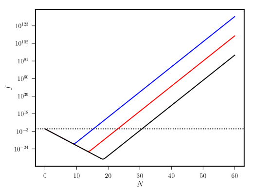
ηsubscript𝜂\eta_{\ast} is the time when the coupling function reaches unity, again. This implies that the model remains in the domain of strong coupling for |ηend||η|<d1/3|ηend|subscript𝜂end𝜂superscript𝑑13subscript𝜂end|\eta_{\rm end}|\leq|\eta|<d^{-1/3}|\eta_{\rm end}| with the peak of the coupling constant f1d2/5similar-tosuperscript𝑓1superscript𝑑25f^{-1}\sim d^{-2/5}. For similar choice of d𝑑d to be 1020superscript102010^{-20}, we get the domain of strong coupling as 1020Mpc|η|1013superscript1020Mpc𝜂superscript101310^{-20}\,{\rm Mpc}\leq|\eta|\leq 10^{-13} Mpc. Note that the region gets broader with the choice of smaller values of d𝑑d with higher coupling constant fmin1.subscriptsuperscript𝑓1minf^{-1}_{\rm min}. Therefore, it is always preferred to choose the d𝑑d as large as possible. This becomes apparent from Fig. 1.

Compared to the conventional scenario with fη2,proportional-to𝑓superscript𝜂2f\propto\eta^{-2}, the above example thus reduces the problem of strong coupling drastically, as the domain of the strong coupling and the amplitude of the coupling constant fmin1subscriptsuperscript𝑓1minf^{-1}_{\rm min} gets smaller than before. The above example also shows that, compared to the Mpc scales, ηsubscript𝜂\eta_{\ast} lies very close to the end of inflation. At this time, the modes corresponding to Mpc scales become super horizon and classical, similar to the primordial perturbations. Requiring the modes corresponding to the Mpc length scales leave the Hubble radius before the model enters into the region of strong coupling weakly provides the lower bound of d𝑑d as 1060.similar-toabsentsuperscript1060\sim 10^{-60}. Since the strong coupling problem relates to whether the quantum origin of the EM field can be trusted, one can argue that, for 1060<d<1020,superscript1060𝑑superscript102010^{-60}<d<10^{-20}, the problem does not arise as the observable modes become classical, thus such choice of coupling function solves the strong coupling problem for modes of Mpc scale.
Refer to caption
Figure 1: The proposed coupling function is plotted against the inflationary e-folding number N𝑁N. 0 denotes the end of inflation, whereas positive N𝑁N values denote the earlier past, and blue, red and black curve correspond to d=1020,1030𝑑superscript1020superscript1030d=10^{-20},~{}10^{-30} and 1040superscript104010^{-40}, respectively. From this figure, it is evident that, while in the range ηendηηminsubscript𝜂end𝜂subscript𝜂min\eta_{\rm end}\leq\eta\leq\eta_{\rm min}, the coupling function f𝑓f acts as η2superscript𝜂2\eta^{-2}, it behaves as η3superscript𝜂3\eta^{3} for ηηmin.𝜂subscript𝜂min\eta\geq\eta_{\rm min}. Also, among these three examples, d=1040𝑑superscript1040d=10^{-40} makes the system stay in the strong coupling region (when f<1𝑓1f<1) for the longest period N<30,𝑁30N<30, while the modes corresponding to Mpc scales leave the Hubble horizon N50.similar-to𝑁50N\sim 50.

This is the main result of this work: we introduce a new coupling function, which corresponds to the linear combination of the dual scale-invariant magnetic field solution and find that it can evade the strong coupling problem for modes of Mpc scales, which we are interested in, and simultaneously can produce 1013superscript101310^{-13} G magnetic field in Mpc scales today without any backreaction. In the next section, we will study the effect of such model in higher-order cross-correlation functions.

4 Cross-correlations between magnetic fields and curvature perturbation

In the previous section, we showed that the proposed coupling function can evade the problem of strong coupling for Mpc scales, and at the same time, can provide sufficient seed magnetic field. However, it is evident that, from the study of power spectrum, we are unable to detect new observational information, and therefore, the obvious thing to do is to study the higher-order cross-correlation functions between the magnetic fields and the curvature perturbation. This has been extensively studied in the literature [66, 67, 68, 69, 70, 71, 72]. In this section, we extend the calculation for our model.

Let us start with the quadratic action for the curvature perturbation \mathcal{R} that provides the evolution of the mode functions. The action is

𝒮=d3𝐱dηa2(η)ϵ(2ii),\mathcal{S}_{\mathcal{R}}=\int{\rm d}^{3}{\rm\bf x}\,{\rm d}\eta\,a^{2}(\eta)\,\epsilon\,\left(\mathcal{R}^{\prime}{}^{2}-\partial_{i}\mathcal{R}\partial^{i}\mathcal{R}\right), (4.1)

where, ϵH˙H2italic-ϵ˙𝐻superscript𝐻2\epsilon\equiv-\frac{\dot{H}}{H^{2}} is the slow-roll parameter. We can write the curvature perturbation \mathcal{R} in terms of the mode functions as

(η,𝐱)=d3𝐱(2π)3/2(a^𝐤𝐤(η)ei𝐤.𝐱+a^𝐤𝐤(η)ei𝐤.𝐱)𝜂𝐱superscriptd3𝐱superscript2𝜋32subscript^𝑎𝐤subscript𝐤𝜂superscript𝑒formulae-sequence𝑖𝐤𝐱subscriptsuperscript^𝑎𝐤subscriptsuperscript𝐤𝜂superscript𝑒formulae-sequence𝑖𝐤𝐱\mathcal{R}(\eta,{\rm\bf x})=\int\frac{{\rm d}^{3}{\rm\bf x}}{(2\pi)^{3/2}}\left(\hat{a}_{{\rm\bf k}}\mathcal{R}_{\rm\bf k}(\eta)e^{i{\rm\bf k}.{\rm\bf x}}+\hat{a}^{\dagger}_{{\rm\bf k}}\mathcal{R}^{\ast}_{\rm\bf k}(\eta)e^{-i{\rm\bf k}.{\rm\bf x}}\right) (4.2)

and during slow-roll inflation, the solution of the mode function in leading order slow-roll can be written as

k(η)=12ϵH2k3(1+ikη)eikη.subscript𝑘𝜂12italic-ϵ𝐻2superscript𝑘31𝑖𝑘𝜂superscript𝑒𝑖𝑘𝜂\mathcal{R}_{k}(\eta)=\frac{1}{\sqrt{2\,\epsilon}}\frac{H}{\sqrt{2\,k^{3}}}\left(1+ik\eta\right)e^{-ik\eta}. (4.3)

Now, in order to evaluate the cross-correlations between magnetic fields and curvature perturbation, we first need the interaction Hamiltonian involving the vector fields Aisubscript𝐴𝑖A_{i} and curvature perturbation \mathcal{R}. This can easily be obtained from the third order perturbed Lagrangian as the density of the interaction Hamiltonian int=3subscriptintsubscript3\mathcal{H}_{\rm int}=-\mathcal{L}_{3} (see Refs. [74, 75, 76]):

Hint=12d3𝐱f2(η)[(aH)(Ai+2FijFij)+2iaHAjFij].H_{\rm int}=\frac{1}{2}\int{\rm d}^{3}{\rm\bf x}\,f^{2}(\eta)\left[\left(\mathcal{R}-\frac{\mathcal{R}^{\prime}}{aH}\right)\left(A_{i}^{\prime}{}^{2}+F_{ij}F^{ij}\right)+\frac{2\partial_{i}\mathcal{R}}{aH}A_{j}^{\prime}F^{ij}\right]. (4.4)

The cross-correlation between the magnetic fields and the curvature perturbation in real space is defined as

(η,𝐱)Bi(η,𝐱)Bi(η,𝐱)=d3𝐤1d3𝐤2d3𝐤3(2π)9/2ei(𝐤1+𝐤2+𝐤3).𝐱𝐤1(η)Bi𝐤2(η)B𝐤3i(η),delimited-⟨⟩𝜂𝐱subscript𝐵𝑖𝜂𝐱superscript𝐵𝑖𝜂𝐱superscriptd3subscript𝐤1superscriptd3subscript𝐤2superscriptd3subscript𝐤3superscript2𝜋92superscript𝑒formulae-sequence𝑖subscript𝐤1subscript𝐤2subscript𝐤3𝐱delimited-⟨⟩subscriptsubscript𝐤1𝜂subscript𝐵𝑖subscript𝐤2𝜂subscriptsuperscript𝐵𝑖subscript𝐤3𝜂\displaystyle\left<\mathcal{R}(\eta,{\rm\bf x})B_{i}(\eta,{\rm\bf x})B^{i}(\eta,{\rm\bf x})\right>=\int\frac{{\rm d}^{3}{\rm\bf k}_{1}\,{\rm d}^{3}{\rm\bf k}_{2}\,{\rm d}^{3}{\rm\bf k}_{3}}{\left(2\pi\right)^{9/2}}e^{i({\rm\bf k}_{1}+{\rm\bf k}_{2}+{\rm\bf k}_{3}).{\rm\bf x}}\left<\mathcal{R}_{{\rm\bf k}_{1}}(\eta)B_{i\,{\rm\bf k}_{2}}(\eta)B^{i}_{{\rm\bf k}_{3}}(\eta)\right>, (4.5)

where Bisubscript𝐵𝑖B_{i} is related to the vector field Aisubscript𝐴𝑖A_{i} as in (2.3). 𝐤subscript𝐤\mathcal{R}_{\rm\bf k} and Bi𝐤subscript𝐵𝑖𝐤B_{i\,{\rm\bf k}} are the Fourier modes associated with the curvature perturbation (see Eq. (4.3)) and i-th𝑡th component of the magnetic field, respectively.

In order to compute the higher-order correlation function during inflation, we adopt a very useful and powerful tool of the in-in formalism [77]. In this formalism, the expectation value of an operator 𝒪𝒪\mathcal{O} at time η𝜂\eta is given by

Ω|𝒪(η)|Ω=0|T¯(eiηHint(η)dη)𝒪(η)T(eiηHint(η′′)dη′′)|0,quantum-operator-productΩ𝒪𝜂Ωquantum-operator-product0¯𝑇superscript𝑒𝑖superscriptsubscript𝜂subscript𝐻intsuperscript𝜂differential-dsuperscript𝜂𝒪𝜂𝑇superscript𝑒𝑖superscriptsubscript𝜂subscript𝐻intsuperscript𝜂′′differential-dsuperscript𝜂′′0\left<\Omega\left|\mathcal{O}(\eta)\right|\Omega\right>=\left<0\left|\bar{T}\left(e^{i\int_{-\infty}^{\eta}H_{\rm int}(\eta^{\prime}){\rm d}\eta^{\prime}}\right)\mathcal{O}(\eta)T\left(e^{-i\int_{-\infty}^{\eta}H_{\rm int}(\eta^{\prime\prime}){\rm d}\eta^{\prime\prime}}\right)\right|0\right>, (4.6)

where, |ΩketΩ\left.|\Omega\right> and |0ket0\left.|0\right> are the vacuum of the interaction and free theories, respectively, T𝑇T and T¯¯𝑇\bar{T} are the time and anti time ordering operators, respectively, and Hintsubscript𝐻intH_{\rm int} is the interaction Hamiltonian. Using leading order contribution of the interaction Hamiltonian, the cross-correlation function at the end of inflation, i.e., ηendsubscript𝜂end\eta_{\rm end} can simply be written as [67, 69]

𝐤1(ηend)Bi𝐤2(ηend)B𝐤3i(ηend)=iηiηenddη[𝐤1(ηend)Bi𝐤2(ηend)B𝐤3i(ηend),Hint(η)].delimited-⟨⟩subscriptsubscript𝐤1subscript𝜂endsubscript𝐵𝑖subscript𝐤2subscript𝜂endsubscriptsuperscript𝐵𝑖subscript𝐤3subscript𝜂end𝑖superscriptsubscriptsubscript𝜂isubscript𝜂enddifferential-d𝜂delimited-⟨⟩subscriptsubscript𝐤1subscript𝜂endsubscript𝐵𝑖subscript𝐤2subscript𝜂endsubscriptsuperscript𝐵𝑖subscript𝐤3subscript𝜂endsubscript𝐻int𝜂\displaystyle\left<\mathcal{R}_{{\rm\bf k}_{1}}(\eta_{\rm end})B_{i\,{\rm\bf k}_{2}}(\eta_{\rm end})B^{i}_{{\rm\bf k}_{3}}(\eta_{\rm end})\right>=-i\int_{\eta_{\rm i}}^{\eta_{\rm end}}{\rm d}\eta\left<\left[\mathcal{R}_{{\rm\bf k}_{1}}(\eta_{\rm end})B_{i\,{\rm\bf k}_{2}}(\eta_{\rm end})B^{i}_{{\rm\bf k}_{3}}(\eta_{\rm end}),H_{\rm int}(\eta)\right]\right>.

Now, for simplicity, we define a new quantity GBB(𝐤1,𝐤2,𝐤3)subscript𝐺𝐵𝐵subscript𝐤1subscript𝐤2subscript𝐤3G_{\mathcal{R}BB}({\rm\bf k}_{1},{\rm\bf k}_{2},{\rm\bf k}_{3}) as

𝐤1(ηend)Bi𝐤2(ηend)B𝐤3i(ηend)(2π)3/2GBB(𝐤1,𝐤2,𝐤3)δ3(𝐤1+𝐤2+𝐤3).delimited-⟨⟩subscriptsubscript𝐤1subscript𝜂endsubscript𝐵𝑖subscript𝐤2subscript𝜂endsubscriptsuperscript𝐵𝑖subscript𝐤3subscript𝜂endsuperscript2𝜋32subscript𝐺𝐵𝐵subscript𝐤1subscript𝐤2subscript𝐤3superscript𝛿3subscript𝐤1subscript𝐤2subscript𝐤3\left<\mathcal{R}_{{\rm\bf k}_{1}}(\eta_{\rm end})B_{i\,{\rm\bf k}_{2}}(\eta_{\rm end})B^{i}_{{\rm\bf k}_{3}}(\eta_{\rm end})\right>\equiv\left(2\pi\right)^{-3/2}G_{\mathcal{R}BB}({\rm\bf k}_{1},{\rm\bf k}_{2},{\rm\bf k}_{3})\delta^{3}({\rm\bf k}_{1}+{\rm\bf k}_{2}+{\rm\bf k}_{3}). (4.8)

Then, by using the expression (4) along with the interaction Hamiltonian (4.4), the definition of the mode functions (4.3) and (2.7), and the Wick’s theorem, GBB(𝐤1,𝐤2,𝐤3)subscript𝐺𝐵𝐵subscript𝐤1subscript𝐤2subscript𝐤3G_{\mathcal{R}BB}({\rm\bf k}_{1},{\rm\bf k}_{2},{\rm\bf k}_{3}) can be expressed as

GBB(𝐤1,𝐤2,𝐤3)=i=16𝒢i(𝐤1,𝐤2,𝐤3),subscript𝐺𝐵𝐵subscript𝐤1subscript𝐤2subscript𝐤3superscriptsubscript𝑖16subscript𝒢𝑖subscript𝐤1subscript𝐤2subscript𝐤3G_{\mathcal{R}BB}({\rm\bf k}_{1},{\rm\bf k}_{2},{\rm\bf k}_{3})=\sum_{i=1}^{6}\mathcal{G}_{i}({\rm\bf k}_{1},{\rm\bf k}_{2},{\rm\bf k}_{3}), (4.9)

where six 𝒢𝒢\mathcal{G}’s are defined as

𝒢1(𝐤1,𝐤2,𝐤3)subscript𝒢1subscript𝐤1subscript𝐤2subscript𝐤3\displaystyle\mathcal{G}_{1}({\rm\bf k}_{1},{\rm\bf k}_{2},{\rm\bf k}_{3}) =\displaystyle= i(k12k22k32)k1(ηend)Ak2(ηend)Ak3(ηend)×\displaystyle i\left(k_{1}^{2}-k_{2}^{2}-k_{3}^{2}\right)\mathcal{R}_{k_{1}}(\eta_{\rm end})A_{k_{2}}(\eta_{\rm end})A_{k_{3}}(\eta_{\rm end})\times (4.10)
ηiηenddηf2(η)k1(η)Ak2(η)Ak3(η)+c.c.formulae-sequencesubscriptsuperscriptsubscript𝜂endsubscript𝜂𝑖differential-d𝜂superscript𝑓2𝜂subscriptsuperscriptsubscript𝑘1𝜂subscriptsuperscript𝐴subscript𝑘2𝜂subscriptsuperscript𝐴subscript𝑘3𝜂𝑐𝑐\displaystyle\int^{\eta_{\rm end}}_{\eta_{i}}{\rm d}\eta\,f^{2}(\eta)\mathcal{R}^{\ast}_{k_{1}}(\eta)A^{\ast\prime}_{k_{2}}(\eta)A^{\ast\prime}_{k_{3}}(\eta)+c.c.
𝒢2(𝐤1,𝐤2,𝐤3)subscript𝒢2subscript𝐤1subscript𝐤2subscript𝐤3\displaystyle\mathcal{G}_{2}({\rm\bf k}_{1},{\rm\bf k}_{2},{\rm\bf k}_{3}) =\displaystyle= i(k12k22k32)k1(ηend)Ak2(ηend)Ak3(ηend)×\displaystyle-i\left(k_{1}^{2}-k_{2}^{2}-k_{3}^{2}\right)\mathcal{R}_{k_{1}}(\eta_{\rm end})A_{k_{2}}(\eta_{\rm end})A_{k_{3}}(\eta_{\rm end})\times (4.11)
ηiηenddηf2(η)aHk1(η)Ak2(η)Ak3(η)+c.c.formulae-sequencesubscriptsuperscriptsubscript𝜂endsubscript𝜂𝑖differential-d𝜂superscript𝑓2𝜂𝑎𝐻subscriptsuperscriptsubscript𝑘1𝜂subscriptsuperscript𝐴subscript𝑘2𝜂subscriptsuperscript𝐴subscript𝑘3𝜂𝑐𝑐\displaystyle\int^{\eta_{\rm end}}_{\eta_{i}}{\rm d}\eta\,\frac{f^{2}(\eta)}{aH}\mathcal{R}^{\ast\prime}_{k_{1}}(\eta)A^{\ast\prime}_{k_{2}}(\eta)A^{\ast\prime}_{k_{3}}(\eta)+c.c.
𝒢3(𝐤1,𝐤2,𝐤3)subscript𝒢3subscript𝐤1subscript𝐤2subscript𝐤3\displaystyle\mathcal{G}_{3}({\rm\bf k}_{1},{\rm\bf k}_{2},{\rm\bf k}_{3}) =\displaystyle= i(k22k32+14(k12k22k32)2)k1(ηend)Ak2(ηend)Ak3(ηend)×\displaystyle-i\left(k_{2}^{2}k_{3}^{2}+\frac{1}{4}\left(k_{1}^{2}-k_{2}^{2}-k_{3}^{2}\right)^{2}\right)\mathcal{R}_{k_{1}}(\eta_{\rm end})A_{k_{2}}(\eta_{\rm end})A_{k_{3}}(\eta_{\rm end})\times (4.12)
ηiηenddηf2(η)k1(η)Ak2(η)Ak3(η)+c.c.formulae-sequencesubscriptsuperscriptsubscript𝜂endsubscript𝜂𝑖differential-d𝜂superscript𝑓2𝜂subscriptsuperscriptsubscript𝑘1𝜂subscriptsuperscript𝐴subscript𝑘2𝜂subscriptsuperscript𝐴subscript𝑘3𝜂𝑐𝑐\displaystyle\int^{\eta_{\rm end}}_{\eta_{i}}{\rm d}\eta\,f^{2}(\eta)\mathcal{R}^{\ast}_{k_{1}}(\eta)A^{\ast}_{k_{2}}(\eta)A^{\ast}_{k_{3}}(\eta)+c.c.
𝒢4(𝐤1,𝐤2,𝐤3)subscript𝒢4subscript𝐤1subscript𝐤2subscript𝐤3\displaystyle\mathcal{G}_{4}({\rm\bf k}_{1},{\rm\bf k}_{2},{\rm\bf k}_{3}) =\displaystyle= i(k22k3214(k12k22k32)2)k1(ηend)Ak2(ηend)Ak3(ηend)×\displaystyle i\left(k_{2}^{2}k_{3}^{2}-\frac{1}{4}\left(k_{1}^{2}-k_{2}^{2}-k_{3}^{2}\right)^{2}\right)\mathcal{R}_{k_{1}}(\eta_{\rm end})A_{k_{2}}(\eta_{\rm end})A_{k_{3}}(\eta_{\rm end})\times (4.13)
ηiηenddηf2(η)aHk1(η)Ak2(η)Ak3(η)+c.c.formulae-sequencesubscriptsuperscriptsubscript𝜂endsubscript𝜂𝑖differential-d𝜂superscript𝑓2𝜂𝑎𝐻subscriptsuperscriptsubscript𝑘1𝜂subscriptsuperscript𝐴subscript𝑘2𝜂subscriptsuperscript𝐴subscript𝑘3𝜂𝑐𝑐\displaystyle\int^{\eta_{\rm end}}_{\eta_{i}}{\rm d}\eta\,\frac{f^{2}(\eta)}{aH}\mathcal{R}^{\ast\prime}_{k_{1}}(\eta)A^{\ast}_{k_{2}}(\eta)A^{\ast}_{k_{3}}(\eta)+c.c.
𝒢5(𝐤1,𝐤2,𝐤3)subscript𝒢5subscript𝐤1subscript𝐤2subscript𝐤3\displaystyle\mathcal{G}_{5}({\rm\bf k}_{1},{\rm\bf k}_{2},{\rm\bf k}_{3}) =\displaystyle= i(k22k32+14(k12k22k32)(k12+3k32k22))k1(ηend)Ak2(ηend)Ak3(ηend)×\displaystyle i\left(k_{2}^{2}k_{3}^{2}+\frac{1}{4}\left(k_{1}^{2}-k_{2}^{2}-k_{3}^{2}\right)\left(k_{1}^{2}+3k_{3}^{2}-k_{2}^{2}\right)\right)\mathcal{R}_{k_{1}}(\eta_{\rm end})A_{k_{2}}(\eta_{\rm end})A_{k_{3}}(\eta_{\rm end})\times (4.14)
ηiηenddηf2(η)aHk1(η)Ak2(η)Ak3(η)+c.c.formulae-sequencesubscriptsuperscriptsubscript𝜂endsubscript𝜂𝑖differential-d𝜂superscript𝑓2𝜂𝑎𝐻subscriptsuperscriptsubscript𝑘1𝜂subscriptsuperscript𝐴subscript𝑘2𝜂subscriptsuperscript𝐴subscript𝑘3𝜂𝑐𝑐\displaystyle\int^{\eta_{\rm end}}_{\eta_{i}}{\rm d}\eta\,\frac{f^{2}(\eta)}{aH}\mathcal{R}^{\ast}_{k_{1}}(\eta)A^{\ast\prime}_{k_{2}}(\eta)A^{\ast}_{k_{3}}(\eta)+c.c.
𝒢6(𝐤1,𝐤2,𝐤3)subscript𝒢6subscript𝐤1subscript𝐤2subscript𝐤3\displaystyle\mathcal{G}_{6}({\rm\bf k}_{1},{\rm\bf k}_{2},{\rm\bf k}_{3}) =\displaystyle= i(k22k32+14(k12k22k32)(k12+3k32k22))k1(ηend)Ak2(ηend)Ak3(ηend)×\displaystyle i\left(k_{2}^{2}k_{3}^{2}+\frac{1}{4}\left(k_{1}^{2}-k_{2}^{2}-k_{3}^{2}\right)\left(k_{1}^{2}+3k_{3}^{2}-k_{2}^{2}\right)\right)\mathcal{R}_{k_{1}}(\eta_{\rm end})A_{k_{2}}(\eta_{\rm end})A_{k_{3}}(\eta_{\rm end})\times (4.15)
ηiηenddηf2(η)aHk1(η)Ak2(η)Ak3(η)+c.c.formulae-sequencesubscriptsuperscriptsubscript𝜂endsubscript𝜂𝑖differential-d𝜂superscript𝑓2𝜂𝑎𝐻subscriptsuperscriptsubscript𝑘1𝜂subscriptsuperscript𝐴subscript𝑘2𝜂subscriptsuperscript𝐴subscript𝑘3𝜂𝑐𝑐\displaystyle\int^{\eta_{\rm end}}_{\eta_{i}}{\rm d}\eta\,\frac{f^{2}(\eta)}{aH}\mathcal{R}^{\ast}_{k_{1}}(\eta)A^{\ast}_{k_{2}}(\eta)A^{\ast\prime}_{k_{3}}(\eta)+c.c.

The abbreviated form of c.cformulae-sequence𝑐𝑐c.c is complex conjugate. Now, given the coupling function f(η)𝑓𝜂f(\eta), which fixes the solution of the vector field A𝐤(η)subscript𝐴𝐤𝜂A_{\rm\bf k}(\eta), and the solution of the curvature perturbation 𝐤subscript𝐤\mathcal{R}_{\rm\bf k}, one can easily compute the cross-correlations using the above expressions.

In our case, with the coupling function (3.2), and the solution of the vector field A𝐤subscript𝐴𝐤A_{{\rm\bf k}}, i.e.,

Ak(η)eikη2k(d(ηηend)51)(3+3ikηk2η2)k2η2similar-to-or-equalssubscript𝐴𝑘𝜂superscript𝑒𝑖𝑘𝜂2𝑘𝑑superscript𝜂subscript𝜂end5133𝑖𝑘𝜂superscript𝑘2superscript𝜂2superscript𝑘2superscript𝜂2A_{k}(\eta)\simeq\frac{e^{-ik\eta}}{\sqrt{2\,k}}\left(d\left(\frac{\eta}{\eta_{\rm end}}\right)^{5}-1\right)\frac{\left(3+3ik\eta-k^{2}\eta^{2}\right)}{k^{2}\eta^{2}}

as well as the solution of the curvature perturbations 𝐤subscript𝐤\mathcal{R}_{\rm\bf k} (4.3), we have evaluated all 𝒢𝒢\mathcal{G}’s, and the explicit expressions are given in Appendix A. Please note that, in doing such evaluations, we assume that d1much-less-than𝑑1d\ll 1, which is evident from Sec. 3.1.

At this point, please notice the logarithmic dependence of 𝒢3subscript𝒢3\mathcal{G}_{3} and 𝒢4subscript𝒢4\mathcal{G}_{4}. Also, in all expressions of 𝒢𝒢\mathcal{G}’s, ηendsubscript𝜂end\eta_{\rm end} appears in the denominator. In 𝒢3subscript𝒢3\mathcal{G}_{3} and 𝒢4subscript𝒢4\mathcal{G}_{4}, while it is ηend4superscriptsubscript𝜂end4\eta_{\rm end}^{4}, in other four 𝒢𝒢\mathcal{G}’s, it appears as ηend6superscriptsubscript𝜂end6\eta_{\rm end}^{6}. Later, while evaluating the non-Gaussianity parameter in the next section, we will show that, while ηend4superscriptsubscript𝜂end4\eta_{\rm end}^{4} dependence cancels out, ηend6superscriptsubscript𝜂end6\eta_{\rm end}^{6} as well as the logarithmic dependencies, in general, do not. And therefore, for ηend0subscript𝜂end0\eta_{\rm end}\rightarrow 0 limit, except for the case of squeezed limit, it contributes enormously in evaluating the non-Gaussianity parameter.

5 Non-Gaussianity parameter

In the last section, we have defined the cross-correlation function between the magnetic fields and the curvature perturbation. However, it is not dimensionless, and therefore, to characterize the correlation function more prominently, we introduce the non-Gaussianity parameter bNLsubscript𝑏NLb_{\rm NL}. The parameter is dimensionless and captures the shape and amplitude of the three-point cross-correlation function discussed in the previous section.

The non-Gaussianity parameter bNLsubscript𝑏NLb_{\rm NL} in the local form is defined as

B^i𝐤(η)=B^i𝐤(G)(η)+bNLd3𝐤(2π)3/2^𝐤𝐤(G)(η)B^i𝐤(G)(η),subscript^𝐵𝑖𝐤𝜂superscriptsubscript^𝐵𝑖𝐤G𝜂subscript𝑏NLsuperscriptd3superscript𝐤superscript2𝜋32subscriptsuperscript^G𝐤superscript𝐤𝜂superscriptsubscript^𝐵𝑖superscript𝐤G𝜂\displaystyle\hat{B}_{i\,\bf k}(\eta)=\hat{B}_{i\,\bf{k}}^{({\rm G})}(\eta)+b_{\rm NL}\,\int\frac{{\rm d}^{3}{\bf k^{\prime}}}{(2\,\pi)^{3/2}}\,\hat{\mathcal{R}}^{(\rm G)}_{\bf{k}-\bf{k^{\prime}}}(\eta)\,\hat{B}_{i\,{\bf k^{\prime}}}^{({\rm G})}(\eta), (5.1)

where B^i𝐤(η)subscript^𝐵𝑖𝐤𝜂\hat{B}_{i\,\bf k}(\eta) is the Fourier model of the magnetic field and (G)𝐺(G) denotes the Gaussian part of the Fourier mode. Using the above expression, one can now evaluate the cross-correlation function (4.8) that interests us and then compare with the same that leads to

bNL(𝐤1,𝐤2,𝐤3)=f2(ηend)8π4a4(ηend)k13k23k33GBB(𝐤1,𝐤2,𝐤3)𝒫(𝐤1)(k32𝒫B(𝐤2)+k22𝒫B(𝐤3)),subscript𝑏NLsubscript𝐤1subscript𝐤2subscript𝐤3superscript𝑓2subscript𝜂end8superscript𝜋4superscript𝑎4subscript𝜂endsuperscriptsubscript𝑘13superscriptsubscript𝑘23superscriptsubscript𝑘33subscript𝐺𝐵𝐵subscript𝐤1subscript𝐤2subscript𝐤3subscript𝒫subscript𝐤1superscriptsubscript𝑘32subscript𝒫Bsubscript𝐤2superscriptsubscript𝑘22subscript𝒫Bsubscript𝐤3b_{\rm NL}({\rm\bf k}_{1},{\rm\bf k}_{2},{\rm\bf k}_{3})=-\frac{f^{2}(\eta_{\rm end})}{8\pi^{4}a^{4}(\eta_{\rm end})}\frac{k_{1}^{3}k_{2}^{3}k_{3}^{3}\,G_{\mathcal{R}BB}({\rm\bf k}_{1},{\rm\bf k}_{2},{\rm\bf k}_{3})}{\mathcal{P}_{\mathcal{R}}({\rm\bf k}_{1})\left(k_{3}^{2}\mathcal{P}_{\rm B}({\rm\bf k}_{2})+k_{2}^{2}\mathcal{P}_{\rm B}({\rm\bf k}_{3})\right)}, (5.2)

where, 𝒫Bsubscript𝒫B\mathcal{P}_{\rm B} is defined in (2.14)italic-(2.14italic-)\eqref{eq:MagSpec} and 𝒫(𝐤)subscript𝒫𝐤\mathcal{P}_{\mathcal{R}({\rm\bf k})} is the power spectrum of the curvature perturbation, defined as

𝒫(𝐤)k32π2|𝐤|2.subscript𝒫𝐤superscript𝑘32superscript𝜋2superscriptsubscript𝐤2\mathcal{P}_{\mathcal{R}}({\rm\bf k})\equiv\frac{k^{3}}{2\pi^{2}}\left|\mathcal{R}_{{\rm\bf k}}\right|^{2}.

At the end of inflation, both the spectra, in our case, take the form

𝒫(𝐤)H28π2ϵ𝒫B(𝐤)9H24π2.formulae-sequencesubscript𝒫𝐤superscript𝐻28superscript𝜋2italic-ϵsubscript𝒫B𝐤9superscript𝐻24superscript𝜋2\mathcal{P}_{\mathcal{R}}({\rm\bf k})\approx\frac{H^{2}}{8\pi^{2}\,\epsilon}\qquad\mathcal{P}_{\rm B}({\rm\bf k})\approx\frac{9H^{2}}{4\pi^{2}}. (5.3)

With the help of the above spectra, along with the six 𝒢𝒢\mathcal{G}’s given in Appendix A, one can easily evaluate bNLsubscript𝑏NLb_{\rm NL}. Since, the expression is enormous, as obvious from the Appendix A, one can simply obtain the same in the three interesting limits: squeezed, equilateral and flattened and study it extensively.

5.1 Squeezed limit

In the squeezed limit, one of the wavenumber is significantly smaller than the other two. Since the wavevctors form a triangle configuration as 𝐤1+𝐤2+𝐤3=0subscript𝐤1subscript𝐤2subscript𝐤30{\rm\bf k}_{1}+{\rm\bf k}_{2}+{\rm\bf k}_{3}=0, 𝐤10subscript𝐤10{\rm\bf k}_{1}\rightarrow 0 implies that 𝐤2=𝐤3subscript𝐤2subscript𝐤3{\rm\bf k}_{2}=-{\rm\bf k}_{3}. In this limit, the non-Gaussianity parameter becomes:

lim𝐤10bNLsq(𝐤1,𝐤,𝐤)subscriptsubscript𝐤10subscriptsuperscript𝑏sqNLsubscript𝐤1𝐤𝐤\displaystyle\lim\limits_{{\rm\bf k}_{1}\rightarrow 0}b^{\rm sq}_{\rm NL}({\rm\bf k}_{1},{\rm\bf k},-{\rm\bf k}) =\displaystyle= limkηend03(6+k2ηend2)9+3k2ηend2+k4ηend4=2.subscript𝑘subscript𝜂end036superscript𝑘2superscriptsubscript𝜂end293superscript𝑘2superscriptsubscript𝜂end2superscript𝑘4superscriptsubscript𝜂end42\displaystyle\lim\limits_{-k\eta_{\rm end}\rightarrow 0}\,\frac{3(6+k^{2}\eta_{\rm end}^{2})}{9+3k^{2}\eta_{\rm end}^{2}+k^{4}\eta_{\rm end}^{4}}=2. (5.4)

Two things to note: bNLsubscript𝑏NLb_{\rm NL} is independent of d𝑑d and k𝑘k. The result is not surprising as it is expected because of the consistency condition which is satisfied during inflation [68, 69]. It tells us that, in the squeezed limit, the non-Gaussianity parameter can be written as the spectral index of the magnetic field energy density as

bNLsq(𝐤1,𝐤,𝐤)=4nB2,subscriptsuperscript𝑏sqNLsubscript𝐤1𝐤𝐤4subscript𝑛B2b^{\rm sq}_{\rm NL}({\rm\bf k}_{1},{\rm\bf k},-{\rm\bf k})=\frac{4-n_{\rm B}}{2},

where,

nBdln𝒫Bdlnk.subscript𝑛Bdsubscript𝒫Bd𝑘n_{\rm B}\equiv\frac{{\rm d}\ln\mathcal{P}_{\rm B}}{{\rm d}\ln k}.

Since, the choice of the coupling function (3.2) leads to scale-invariant magnetic field spectrum, the corresponding spectral index nBsubscript𝑛Bn_{\rm B} is zero, which makes bNLsubscript𝑏NLb_{\rm NL} to be equal to two.

The relation has previously been obtained with the help of power-law kind of coupling function, i.e., f(η)αproportional-to𝑓superscript𝜂𝛼f\propto(-\eta)^{\alpha} [64, 65]. However, although the magnetic spectrum is scale-invariant, our proposed coupling function is not power-law, and even after that, with this new choice (3.2), we obtain the result: consistency relation is satisfied. The result is interesting and unique as in the next section, it will be apparent that in the other limits, the non-Gaussianity parameter depends both on k𝑘k and d𝑑d. This is another interesting result of this work.

5.2 Equilateral limit

Unlike the squeezed limit, in the equilateral limit, the non-Gaussianity parameter behaves differently and possesses unique signatures. In this limit, as it forms equilateral triangle, it implies k1=k2=k3subscript𝑘1subscript𝑘2subscript𝑘3k_{1}=k_{2}=k_{3}. In this configuration, the non-Gaussianity parameter acts as

bNLeq(k,k,k)=4.112.37dk2ηend22.62log|kηend|.subscriptsuperscript𝑏eqNL𝑘𝑘𝑘4.112.37𝑑superscript𝑘2superscriptsubscript𝜂end22.62𝑘subscript𝜂end\displaystyle b^{\rm eq}_{\rm NL}(k,k,k)=4.11-\frac{2.37\,d}{k^{2}\eta_{\rm end}^{2}}-2.62\log|k\eta_{\rm end}|. (5.5)

Such form of non-Gaussianity parameter is unique: it contains two kinds of ηendsubscript𝜂end\eta_{\rm end} dependence. One kind appears with the parameter d𝑑d in the denominator, while the other enters into the logarithmic. The logarithmic dependence is natural and explored before for f(η)2proportional-to𝑓superscript𝜂2f\propto(-\eta)^{-2}, while the former one is unexplored to date.

The above expression also provides us an interesting scenario: for a given wavenumber, bNLsubscript𝑏NLb_{\rm NL} vanishes at dk2ηend2log|kηend|similar-to-or-equalssubscript𝑑superscript𝑘2superscriptsubscript𝜂end2𝑘subscript𝜂endd_{\ast}\simeq-k^{2}\eta_{\rm end}^{2}\log|k\eta_{\rm end}|. When d>d𝑑subscript𝑑d>d_{\ast}, the non-Gaussian parameter becomes negative and entirely behaves as

bNLeq2.37dk2ηend2.similar-to-or-equalssubscriptsuperscript𝑏eqNL2.37𝑑superscript𝑘2superscriptsubscript𝜂end2b^{\rm eq}_{\rm NL}\simeq-\frac{2.37\,d}{k^{2}\eta_{\rm end}^{2}}.

For d>d,𝑑subscript𝑑d>d_{\ast}, it becomes positive and independent of d𝑑d, and quickly reaches to the saturated value

bNLeq2.62log|kηend|.similar-to-or-equalssubscriptsuperscript𝑏eqNL2.62𝑘subscript𝜂endb^{\rm eq}_{\rm NL}\simeq-2.62\,\log|k\eta_{\rm end}|.

This is plotted in Fig. 2.

Refer to caption
Refer to caption
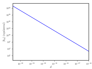
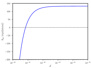
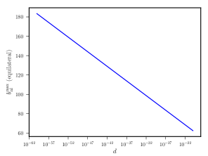
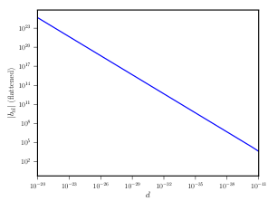
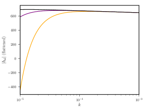
Figure 2: bNLeqsubscriptsuperscript𝑏eqNLb^{\rm eq}_{\rm NL} is plotted against d𝑑d for the pivot scale k=0.05𝑘0.05k=0.05 Mpc. For d>1041,𝑑superscript1041d>10^{-41}, it behaves as dproportional-toabsent𝑑\propto d, whereas, for d<1041𝑑superscript1041d<10^{-41}, it quickly saturates at 132.132132.

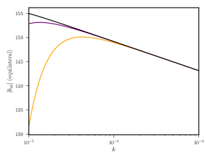
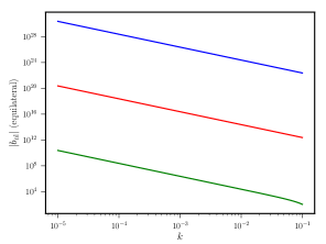
In Fig. 3, for different values of d𝑑d, we plot the bNLsubscript𝑏NLb_{\rm NL} in the equilateral limit. As obvious from (5.5), for a given value of k𝑘k such that d>k2ηend2log|kηend|,𝑑superscript𝑘2superscriptsubscript𝜂end2𝑘subscript𝜂endd>-k^{2}\eta_{\rm end}^{2}\log|k\eta_{\rm end}|, then the non-Gaussianity parameter behaves as k2,proportional-toabsentsuperscript𝑘2\propto k^{-2}, whereas, for d>k2ηend2log|kηend|,𝑑superscript𝑘2superscriptsubscript𝜂end2𝑘subscript𝜂endd>-k^{2}\eta_{\rm end}^{2}\log|k\eta_{\rm end}|, it becomes positive and possesses a maximum at

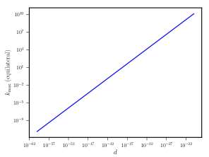
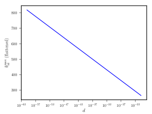
kmax=1.34dηend,bNLmax=2.79+0.608d2.62log[1.34d].formulae-sequencesubscript𝑘max1.34𝑑subscript𝜂endsubscriptsuperscript𝑏maxNL2.790.608𝑑2.621.34𝑑k_{\rm max}=-\frac{1.34\sqrt{d}}{\eta_{\rm end}},\quad b^{\rm max}_{\rm NL}=2.79+0.608\,d-2.62\,\log[1.34\,\sqrt{d}].

After that, it becomes independent of d𝑑d and behaves logarithmic. In Fig. 4, kmaxsubscript𝑘maxk_{\rm max} and bNLmaxsubscriptsuperscript𝑏maxNLb^{\rm max}_{\rm NL} is plotted against d𝑑d. It becomes apparent that, in equilateral limit, bNLmax𝒪(2).similar-tosubscriptsuperscript𝑏maxNL𝒪2b^{\rm max}_{\rm NL}\sim\mathcal{O}(2).
Refer to caption
Refer to caption
Figure 3: We plot bNLeqsubscriptsuperscript𝑏eq𝑁𝐿b^{\rm eq}_{NL} against k𝑘k for different values of d𝑑d (blue for 1020,superscript102010^{-20}, red for d=1030,𝑑superscript1030d=10^{-30}, green for d=1040𝑑superscript1040d=10^{-40}, orange for d=1049𝑑superscript1049d=10^{-49}, purple for d=1050𝑑superscript1050d=10^{-50} and black for 1051superscript105110^{-51}).
Refer to caption
Refer to caption
Figure 4: In the left, we plot kmaxdproportional-tosubscript𝑘max𝑑k_{\rm max}\propto\sqrt{d} against d𝑑d in the equilateral limit. In the right, we plot bNLmaxsubscriptsuperscript𝑏maxNLb^{\rm max}_{\rm NL} against d𝑑d. As one can see, the maximum value of the non-Gaussianity parameter decreases with d𝑑d.

From these figures, it is now obvious that the in the equilateral limit, the non-Gaussianity parameter corresponding to the pivot scale can be as large as 1023superscript102310^{23} to zero, depending on the value of the model parameter d𝑑d, which is huge and never explored.

5.3 Flattened limit

The flattened limit implies that k1=2k2=2k3subscript𝑘12subscript𝑘22subscript𝑘3k_{1}=2k_{2}=2k_{3}, and in this limit, similar to equilateral limit, bNLsubscript𝑏NLb_{\rm NL} behaves as

bNLfl=12.7115.6dk2ηend212log|kηend|subscriptsuperscript𝑏flNL12.7115.6𝑑superscript𝑘2superscriptsubscript𝜂end212𝑘subscript𝜂endb^{\rm fl}_{\rm NL}=12.7-\frac{115.6\,d}{k^{2}\eta_{\rm end}^{2}}-12\log|k\eta_{\rm end}| (5.6)

Again, similar to equilateral limit, for d=d0.1k2ηend2log|kηend|𝑑subscript𝑑similar-to-or-equals0.1superscript𝑘2superscriptsubscript𝜂end2𝑘subscript𝜂endd=d_{\ast}\simeq-0.1\,k^{2}\eta_{\rm end}^{2}\,\log|k\eta_{\rm end}|, the non-Gaussianity parameter vanishes. For d𝑑d greater than that value, it behaves as

115.6dk2ηend2,115.6𝑑superscript𝑘2superscriptsubscript𝜂end2-\frac{115.6\,d}{k^{2}\eta_{\rm end}^{2}},

while for d<d𝑑subscript𝑑d<d_{\ast}, it behaves as

12log|kηend|.12𝑘subscript𝜂end-12\log|k\eta_{\rm end}|.

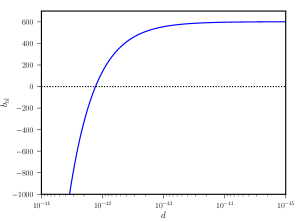
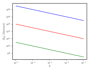
Such dependencies of bNLflsubscriptsuperscript𝑏flNLb^{\rm fl}_{\rm NL} have been plotted in Fig. 5 and Fig. 6. Also, kmaxsubscript𝑘maxk_{\rm max} and bNLmaxsubscriptsuperscript𝑏maxNLb^{\rm max}_{\rm NL} for this case yield as

kmax4.39dηend,bLmax6.7540.67d12log[4.38d].formulae-sequencesimilar-to-or-equalssubscript𝑘max4.39𝑑subscript𝜂endsimilar-to-or-equalssubscriptsuperscript𝑏maxL6.7540.67𝑑124.38𝑑k_{\rm max}\simeq-4.39\frac{\sqrt{d}}{\eta_{\rm end}},\quad b^{\rm max}_{\rm L}\simeq 6.75-40.67\,d-12\log[4.38\sqrt{d}].
Refer to caption
Refer to caption
Figure 5: bNLflsubscriptsuperscript𝑏flNLb^{\rm fl}_{\rm NL} is plotted against d𝑑d for the pivot scale k=0.05𝑘0.05k=0.05 Mpc. For d>1041,𝑑superscript1041d>10^{-41}, it behaves as dproportional-toabsent𝑑\propto d, whereas, for d<1041𝑑superscript1041d<10^{-41}, it quickly saturates at 600.similar-toabsent600\sim 600.
Refer to caption
Refer to caption
Figure 6: We plot bNLflsubscriptsuperscript𝑏fl𝑁𝐿b^{\rm fl}_{NL} against k𝑘k for different values of d𝑑d (blue for 1020,superscript102010^{-20}, red for d=1030,𝑑superscript1030d=10^{-30}, green for d=1040𝑑superscript1040d=10^{-40}, orange for d=1049𝑑superscript1049d=10^{-49}, purple for d=1050𝑑superscript1050d=10^{-50} and black for 1051superscript105110^{-51}).
Refer to caption
Refer to caption
Figure 7: In the left, we plot kmaxdproportional-tosubscript𝑘max𝑑k_{\rm max}\propto\sqrt{d} against d𝑑d in the equilateral limit. In the right, we plot bNLmaxsubscriptsuperscript𝑏maxNLb^{\rm max}_{\rm NL} against d𝑑d. As one can see, the maximum value of the non-Gaussianity parameter decreases with d𝑑d.

These have been plotted in Fig. 7. From these figure, it becomes apparent that the non-Gaussianity parameter in flattened limit always generate higher value than that in the equilateral limit. For d>d𝑑subscript𝑑d>d_{\ast}, the ratio between them, i.e., bNLfl/bNLeq50similar-tosubscriptsuperscript𝑏flNLsubscriptsuperscript𝑏eqNL50b^{\rm fl}_{\rm NL}/b^{\rm eq}_{\rm NL}\sim 50, whereas, for d<d,𝑑subscript𝑑d<d_{\ast}, it is 4.6similar-toabsent4.6\sim 4.6.

Similar to the equilateral limit, it is now obvious that the in the flattened limit, the non-Gaussianity parameter corresponding to the pivot scale can be as large as 1024superscript102410^{24} to zero, depending on the value of the model parameter d𝑑d. This is another interesting result of our work.

6 Conclusions

Inflationary magnetogenesis has long been studied in the literature that can explain the current magnetic field abundances in the cosmic scales. In doing so, many mechanisms have been proposed and among them, 1/4f2(ϕ)FμνFμν14superscript𝑓2italic-ϕsubscript𝐹𝜇𝜈superscript𝐹𝜇𝜈-1/4f^{2}(\phi)F_{\mu\nu}F^{\mu\nu} model grabs the most attention. At present time, it can safely generate 1013superscript101310^{-13} G at Mpc length scale. For two kinds of coupling function solutions, this can be achieved. However, both of them suffer severe issues: while one leads to high electric field energy density that can spoil the background and the model cannot self-sustain, another leads to what is referred to as the strong coupling problem. In this case, the coupling function, at the beginning of inflation possesses a very tiny value 1much-less-thanabsent1\ll 1, which implies that the effective coupling constant is extremely high, i.e., 1much-greater-thanabsent1\gg 1 which, in turn, makes the quantization process of the vector field theory untrustworthy. Due to these issues, one can show that such model can generate not more than 1030superscript103010^{-30} G magnetic field self-consistently in the Mpc length scales [44].

We noticed that, although each of the scale-invariant solutions suffers from backreaction or the strong coupling, each of them also solves the other problem, i.e., the solution with strong coupling does not possess backreaction and vice-versa. Motivated by this, we proposed a new coupling function which is a linear combination of both the coupling functions. In doing so, we introduce a model parameter that characterizes the linear combination and showed that, in order to evade the backreaction problem, one finds the value to be extremely small i.e., d1020.less-than-or-similar-to𝑑superscript1020d\lesssim 10^{-20}. We also found that, for such model with a non-zero value of d𝑑d, it contains two distinct regions:

  • 1.

    for |η|d1/3|ηend|,greater-than-or-equivalent-to𝜂superscript𝑑13subscript𝜂end|\eta|\gtrsim d^{-1/3}|\eta_{\rm end}|, there is no strong coupling,

  • 2.

    for |ηend||η|d1/3|ηend|,less-than-or-similar-tosubscript𝜂end𝜂less-than-or-similar-tosuperscript𝑑13subscript𝜂end|\eta_{\rm end}|\lesssim|\eta|\lesssim d^{-1/3}\,|\eta_{\rm end}|, the model enters into the strong coupling region.

Assuming the pivot scale k=0.05𝑘0.05k=0.05 Mpc-1 exiting the Hubble horizon 50 e-folds before the end of inflation, we find that, for 1020d1060less-than-or-similar-tosuperscript1020𝑑less-than-or-similar-tosuperscript106010^{-20}\lesssim d\lesssim 10^{-60}, the modes corresponding to the Mpc length scales become super-Horizon and classical, similar to inflationary perturbations before the system enters into the strong coupling region. Therefore, one can argue that, while very short wavelength modes suffer the problem of strong coupling, the high wavelength modes that we are interested in do not suffer the same, thus solving the problem of strong coupling for primordial magnetogenesis. In this way, we showed that, today, up to 1013superscript101310^{-13} G strength of the magnetic field can be generated self-consistently in the Mpc scales, which earlier was only 1030similar-toabsentsuperscript1030\sim 10^{-30} G [78, 64, 65].

We, further extended our work to find the non-Gaussian signature of this model. We found that the model satisfies the consistency relation, i.e., in the squeezed limit, the non-Gaussianity parameter can be written in terms of the magnetic field spectra index as bNL=(4n)/2.subscript𝑏NL4𝑛2b_{\rm NL}=(4-n)/2. We also found the unique signatures of bNLsubscript𝑏NLb_{\rm NL} in the equilateral and flattened limit as:

bNL(k)C1dk2ηend2C2log|kηend|.similar-tosubscript𝑏NL𝑘subscript𝐶1𝑑superscript𝑘2superscriptsubscript𝜂end2subscript𝐶2𝑘subscript𝜂endb_{\rm NL}(k)\sim-C_{1}\frac{d}{k^{2}\eta_{\rm end}^{2}}-C_{2}\log|k\eta_{\rm end}|.

For a certain range of k𝑘k, while it is negative and k2proportional-toabsentsuperscript𝑘2\propto k^{-2}, for the rest, it becomes positive and log|kηend|proportional-toabsent𝑘subscript𝜂end\propto\log|k\eta_{\rm end}| with the flattened limit producing greater amplitude than the same in equilateral limit. This implies that the non-Gaussianity parameter can be as high as 1020superscript102010^{20} and as small as 𝒪(1)𝒪1\mathcal{O}(1) depending on the model parameter d𝑑d. These unique signatures can easily be verified from the future experiments which can detect these kinds of non-linearity.

The scope of such model is huge. One immediate extension is to study the effect of similar coupling functions in the context of helical magnetic field generation, which has been studied with the help of the auxiliary scalar field in Ref. [72]. Inflationary Universe, too, suffers from many issues, for which, there is a growing interest in finding alternatives to inflation and among them, the classical bouncing scenario is the most popular one. It would also thus be interesting to investigate the effect of such coupling function in the bouncing scenario. Recently, in Ref. [71], it has been extensively studied with the help of simple auxiliary scalar field coupling of fa(η)α.proportional-to𝑓𝑎superscript𝜂𝛼f\propto a(\eta)^{\alpha}. The auxiliary field has been used due to the fact that the curvature perturbations in the bouncing model do not satisfy the observational constraint. However, in Refs. [79, 80], with the help of non-minimal coupling, the first viable bouncing model has been constructed (also see Refs. [81, 82, 83] in these regard). These works are now in progress.

Acknowledgements

The author wishes to thank L. Sriramkumar and Kinjalk Lochan for useful discussion. The author also thanks Sagarika Tripathy for the help in evaluating the non-Gaussian parameter.

Appendix A Evaluating the 𝒢𝒢\mathcal{G}’s

𝒢1(𝐤1,𝐤2,𝐤3)subscript𝒢1subscript𝐤1subscript𝐤2subscript𝐤3\displaystyle\mathcal{G}_{1}({\rm\bf k}_{1},{\rm\bf k}_{2},{\rm\bf k}_{3}) =\displaystyle= H28ϵk13k25k35kT6ηend6(k12k22k32)(k22k32kT4ηend2(9(k13+2k12(k2+k3)+\displaystyle-\frac{H^{2}}{8\,\epsilon\,k_{1}^{3}\,k_{2}^{5}\,k_{3}^{5}\,k_{T}^{6}\,\eta_{\rm end}^{6}}(k_{1}^{2}-k_{2}^{2}-k_{3}^{2})(k_{2}^{2}k_{3}^{2}k_{T}^{4}\eta_{\rm end}^{2}(-9(k_{1}^{3}+2k_{1}^{2}(k_{2}+k_{3})+ (A.1)
2k1(k22+k2k3+k32)+(k2+k3)(k22+k2k3+k32))3(2k1k22k32+\displaystyle 2k_{1}(k_{2}^{2}+k_{2}k_{3}+k_{3}^{2})+(k_{2}+k_{3})(k_{2}^{2}+k_{2}k_{3}+k_{3}^{2}))-3(2k_{1}k_{2}^{2}k_{3}^{2}+
k22k32(k2+k3)+2k13(k22+k32)+2k12(k2+k3)(k22+k2k3+k32))ηend2+\displaystyle k_{2}^{2}k_{3}^{2}(k_{2}+k_{3})+2k_{1}^{3}(k_{2}^{2}+k_{3}^{2})+2k_{1}^{2}(k_{2}+k_{3})(k_{2}^{2}+k_{2}k_{3}+k_{3}^{2}))\eta_{\rm end}^{2}+
k22k32(4k13+2k1k2k3k12(k2+k3)+k2k3(k2+k3))ηend4+limit-fromsuperscriptsubscript𝑘22superscriptsubscript𝑘324superscriptsubscript𝑘132subscript𝑘1subscript𝑘2subscript𝑘3superscriptsubscript𝑘12subscript𝑘2subscript𝑘3subscript𝑘2subscript𝑘3subscript𝑘2subscript𝑘3superscriptsubscript𝜂end4\displaystyle k_{2}^{2}k_{3}^{2}(-4k_{1}^{3}+2k_{1}k_{2}k_{3}-k_{1}^{2}(k_{2}+k_{3})+k_{2}k_{3}(k_{2}+k_{3}))\eta_{\rm end}^{4}+
k12k23k33(k1+k2+k3)ηend6)+5dk12(3(k2+k3)(k24k23k3+k22k32k2k33+\displaystyle k_{1}^{2}k_{2}^{3}k_{3}^{3}(k_{1}+k_{2}+k_{3})\eta_{\rm end}^{6})+5dk_{1}^{2}(-3(k_{2}+k_{3})(k_{2}^{4}-k_{2}^{3}k_{3}+k_{2}^{2}k_{3}^{2}-k_{2}k_{3}^{3}+
k34)(3k24+18k23k3+38k22k32+18k2k33+3k34)ηend2k22k32(k2+k3)3(3k24+\displaystyle k_{3}^{4})(3k_{2}^{4}+18k_{2}^{3}k_{3}+38k_{2}^{2}k_{3}^{2}+18k_{2}k_{3}^{3}+3k_{3}^{4})\eta_{\rm end}^{2}-k_{2}^{2}k_{3}^{2}(k_{2}+k_{3})^{3}(3k_{2}^{4}+
9k23k38k22k32+9k2k33+3k34)ηend4k24k34(k2+k3)5ηend6+3k1(k2+k3)2\displaystyle 9k_{2}^{3}k_{3}-8k_{2}^{2}k_{3}^{2}+9k_{2}k_{3}^{3}+3k_{3}^{4})\eta_{\rm end}^{4}-k_{2}^{4}k_{3}^{4}(k_{2}+k_{3})^{5}\eta_{\rm end}^{6}+3k_{1}(k_{2}+k_{3})^{2}
(9(k2+k3)46(k26+k25k34k24k322k23k334k22k34+k2k35+k36)ηend2\displaystyle(9(k_{2}+k_{3})^{4}-6(k_{2}^{6}+k_{2}^{5}k_{3}-4k_{2}^{4}k_{3}^{2}-2k_{2}^{3}k_{3}^{3}-4k_{2}^{2}k_{3}^{4}+k_{2}k_{3}^{5}+k_{3}^{6})\eta_{\rm end}^{2}-
k22k32(k2+k3)2(k224k2k3+k32)ηend4)+k15(27(k22+k32)+18(k24+k22k32+\displaystyle k_{2}^{2}k_{3}^{2}(k_{2}+k_{3})^{2}(k_{2}^{2}-4k_{2}k_{3}+k_{3}^{2})\eta_{\rm end}^{4})+k_{1}^{5}(27(k_{2}^{2}+k_{3}^{2})+18(k_{2}^{4}+k_{2}^{2}k_{3}^{2}+
k34)ηend2+9k22k32(k22+k32)ηend4+4k24k34ηend6)+3k14(k2+k3)(54(k22+k32)+\displaystyle k_{3}^{4})\eta_{\rm end}^{2}+9k_{2}^{2}k_{3}^{2}(k_{2}^{2}+k_{3}^{2})\eta_{\rm end}^{4}+4k_{2}^{4}k_{3}^{4}\eta_{\rm end}^{6})+3k_{1}^{4}(k_{2}+k_{3})(54(k_{2}^{2}+k_{3}^{2})+
3(7k24+5k23k3+7k22k32+5k2k33+7k34)ηend2+k22k32(11k22+7k2k3+\displaystyle 3(7k_{2}^{4}+5k_{2}^{3}k_{3}+7k_{2}^{2}k_{3}^{2}+5k_{2}k_{3}^{3}+7k_{3}^{4})\eta_{\rm end}^{2}+k_{2}^{2}k_{3}^{2}(11k_{2}^{2}+7k_{2}k_{3}+
11k32)ηend4+5k24k34ηend6)+2k12(k2+k3)(81(k2+k3)4+9(k26+8k25k3\displaystyle 11k_{3}^{2})\eta_{\rm end}^{4}+5k_{2}^{4}k_{3}^{4}\eta_{\rm end}^{6})+2k_{1}^{2}(k_{2}+k_{3})(81(k_{2}+k_{3})^{4}+9(k_{2}^{6}+8k_{2}^{5}k_{3}
+17k24k32+19k23k33+17k22k34+8k2k35+k36)ηend2+3k22k32(3k24+15k23k3\displaystyle+17k_{2}^{4}k_{3}^{2}+19k_{2}^{3}k_{3}^{3}+17k_{2}^{2}k_{3}^{4}+8k_{2}k_{3}^{5}+k_{3}^{6})\eta_{\rm end}^{2}+3k_{2}^{2}k_{3}^{2}(3k_{2}^{4}+15k_{2}^{3}k_{3}
+14k22k32+15k2k33+3k34)ηend4+5k24k34(k2+k3)2ηend6)+2k13(45(3k24+\displaystyle+14k_{2}^{2}k_{3}^{2}+15k_{2}k_{3}^{3}+3k_{3}^{4})\eta_{\rm end}^{4}+5k_{2}^{4}k_{3}^{4}(k_{2}+k_{3})^{2}\eta_{\rm end}^{6})+2k_{1}^{3}(45(3k_{2}^{4}+
9k23k3+8k22k32+9k2k33+3k34)+3(k22+k32)(12k24+45k23k3+56k22k32+\displaystyle 9k_{2}^{3}k_{3}+8k_{2}^{2}k_{3}^{2}+9k_{2}k_{3}^{3}+3k_{3}^{4})+3(k_{2}^{2}+k_{3}^{2})(12k_{2}^{4}+45k_{2}^{3}k_{3}+56k_{2}^{2}k_{3}^{2}+
45k2k33+12k34)ηend2+k22k32(21k24+72k23k3+82k22k32+72k2k33+\displaystyle 45k_{2}k_{3}^{3}+12k_{3}^{4})\eta_{\rm end}^{2}+k_{2}^{2}k_{3}^{2}(21k_{2}^{4}+72k_{2}^{3}k_{3}+82k_{2}^{2}k_{3}^{2}+72k_{2}k_{3}^{3}+
21k34)ηend4+10k24k34(k2+k3)2ηend6))),\displaystyle 21k_{3}^{4})\eta_{\rm end}^{4}+10k_{2}^{4}k_{3}^{4}(k_{2}+k_{3})^{2}\eta_{\rm end}^{6}))),
𝒢2(𝐤1,𝐤2,𝐤3)subscript𝒢2subscript𝐤1subscript𝐤2subscript𝐤3\displaystyle\mathcal{G}_{2}({\rm\bf k}_{1},{\rm\bf k}_{2},{\rm\bf k}_{3}) =\displaystyle= H28ϵk1k25k35kT7ηend6(k12k22k32)(k22k32kT4ηend2(9(k12+3k1(k2+k3)+\displaystyle-\frac{H^{2}}{8\,\epsilon\,k_{1}\,k_{2}^{5}\,k_{3}^{5}\,k_{T}^{7}\,\eta_{\rm end}^{6}}(k_{1}^{2}-k_{2}^{2}-k_{3}^{2})(k_{2}^{2}k_{3}^{2}k_{T}^{4}\eta_{\rm end}^{2}(-9(k_{1}^{2}+3k_{1}(k_{2}+k_{3})+ (A.2)
2(k22+3k2k3+k32))+3(3k1k2k3(k2+k3)+k12(k22+k32)(k22+k32)(k22+\displaystyle 2(k_{2}^{2}+3k_{2}k_{3}+k_{3}^{2}))+3(3k_{1}k_{2}k_{3}(k_{2}+k_{3})+k_{1}^{2}(k_{2}^{2}+k_{3}^{2})-(k_{2}^{2}+k_{3}^{2})(k_{2}^{2}+
3k2k3+k32))ηend2+(3k1k23(k1+k2)2+9k1k23(k1+k2)k3+k22(k1+k2)\displaystyle 3k_{2}k_{3}+k_{3}^{2}))\eta_{\rm end}^{2}+(3k_{1}k_{2}^{3}(k_{1}+k_{2})^{2}+9k_{1}k_{2}^{3}(k_{1}+k_{2})k_{3}+k_{2}^{2}(k_{1}+k_{2})
(8k1+k2)k32+3k1(k12+3k1k2+3k22)k33+(6k12+9k1k2+k22)k34+3k1k35)\displaystyle(8k_{1}+k_{2})k_{3}^{2}+3k_{1}(k_{1}^{2}+3k_{1}k_{2}+3k_{2}^{2})k_{3}^{3}+(6k_{1}^{2}+9k_{1}k_{2}+k_{2}^{2})k_{3}^{4}+3k_{1}k_{3}^{5})
ηend4+k22k32(k1+k2+k3)(2k1k2(k1+k2)+(k1+k2)(2k1+k2)k3+(2k1+\displaystyle\eta_{\rm end}^{4}+k_{2}^{2}k_{3}^{2}(k_{1}+k_{2}+k_{3})(2k_{1}k_{2}(k_{1}+k_{2})+(k_{1}+k_{2})(2k_{1}+k_{2})k_{3}+(2k_{1}+
k2)k32)ηend6)5d(18k13(3k22(k1+k2)2(k1+5k2)+21k22(k1+k2)(k1+5k2)k3+\displaystyle k_{2})k_{3}^{2})\eta_{\rm end}^{6})-5d(18k_{1}^{3}(3k_{2}^{2}(k_{1}+k_{2})^{2}(k_{1}+5k_{2})+21k_{2}^{2}(k_{1}+k_{2})(k_{1}+5k_{2})k_{3}+
(k1+4k2)(3k12+9k1k2+70k22)k32+7(3k12+18k1k2+40k22)k33+3(11k1+\displaystyle(k_{1}+4k_{2})(3k_{1}^{2}+9k_{1}k_{2}+70k_{2}^{2})k_{3}^{2}+7(3k_{1}^{2}+18k_{1}k_{2}+40k_{2}^{2})k_{3}^{3}+3(11k_{1}+
35k2)k34+15k35)+3(21k12(k2+k3)2(k22+k32)(k24+2k23k3+4k22k32+2k2k33+\displaystyle 35k_{2})k_{3}^{4}+15k_{3}^{5})+3(21k_{1}^{2}(k_{2}+k_{3})^{2}(k_{2}^{2}+k_{3}^{2})(k_{2}^{4}+2k_{2}^{3}k_{3}+4k_{2}^{2}k_{3}^{2}+2k_{2}k_{3}^{3}+
k34)+2(k2+k3)2(k24k23k3+k22k32k2k33+k34)(3k24+18k23k3+38k22k32+\displaystyle k_{3}^{4})+2(k_{2}+k_{3})^{2}(k_{2}^{4}-k_{2}^{3}k_{3}+k_{2}^{2}k_{3}^{2}-k_{2}k_{3}^{3}+k_{3}^{4})(3k_{2}^{4}+18k_{2}^{3}k_{3}+38k_{2}^{2}k_{3}^{2}+
18k2k33+3k34)+3k16(7k24+6k22k32+7k34)+3k15(k2+k3)(25k24+24k23k3+\displaystyle 18k_{2}k_{3}^{3}+3k_{3}^{4})+3k_{1}^{6}(7k_{2}^{4}+6k_{2}^{2}k_{3}^{2}+7k_{3}^{4})+3k_{1}^{5}(k_{2}+k_{3})(25k_{2}^{4}+24k_{2}^{3}k_{3}+
18k22k32+24k2k33+25k34)+2k13(k2+k3)(k22+k32)(27k24+120k23k3+\displaystyle 18k_{2}^{2}k_{3}^{2}+24k_{2}k_{3}^{3}+25k_{3}^{4})+2k_{1}^{3}(k_{2}+k_{3})(k_{2}^{2}+k_{3}^{2})(27k_{2}^{4}+120k_{2}^{3}k_{3}+
209k22k32+120k2k33+27k34)+2k14(k22+k32)(48k24+189k23k3+242k22k32+\displaystyle 209k_{2}^{2}k_{3}^{2}+120k_{2}k_{3}^{3}+27k_{3}^{4})+2k_{1}^{4}(k_{2}^{2}+k_{3}^{2})(48k_{2}^{4}+189k_{2}^{3}k_{3}+242k_{2}^{2}k_{3}^{2}+
189k2k33+48k34)+k1(k2+k3)(15k28+48k27k3+34k26k32+92k25k33+22k24k34+\displaystyle 189k_{2}k_{3}^{3}+48k_{3}^{4})+k_{1}(k_{2}+k_{3})(15k_{2}^{8}+48k_{2}^{7}k_{3}+34k_{2}^{6}k_{3}^{2}+92k_{2}^{5}k_{3}^{3}+22k_{2}^{4}k_{3}^{4}+
92k23k35+34k22k36+48k2k37+15k38))ηend2+kT2(9k1k25(k1+k2)4+45k1k25\displaystyle 92k_{2}^{3}k_{3}^{5}+34k_{2}^{2}k_{3}^{6}+48k_{2}k_{3}^{7}+15k_{3}^{8}))\eta_{\rm end}^{2}+k_{T}^{2}(9k_{1}k_{2}^{5}(k_{1}+k_{2})^{4}+45k_{1}k_{2}^{5}
(k1+k2)3k3+3k24(k1+k2)2(13k12+24k1k2+2k22)k32+15k24(k1+k2)superscriptsubscript𝑘1subscript𝑘23subscript𝑘33superscriptsubscript𝑘24superscriptsubscript𝑘1subscript𝑘2213superscriptsubscript𝑘1224subscript𝑘1subscript𝑘22superscriptsubscript𝑘22superscriptsubscript𝑘3215superscriptsubscript𝑘24subscript𝑘1subscript𝑘2\displaystyle(k_{1}+k_{2})^{3}k_{3}+3k_{2}^{4}(k_{1}+k_{2})^{2}(13k_{1}^{2}+24k_{1}k_{2}+2k_{2}^{2})k_{3}^{2}+15k_{2}^{4}(k_{1}+k_{2})
(13k12+2k22)k33+k22(39k14+195k13k2+50k12k22+64k1k23+26k24)k34+13superscriptsubscript𝑘122superscriptsubscript𝑘22superscriptsubscript𝑘33limit-fromsuperscriptsubscript𝑘2239superscriptsubscript𝑘14195superscriptsubscript𝑘13subscript𝑘250superscriptsubscript𝑘12superscriptsubscript𝑘2264subscript𝑘1superscriptsubscript𝑘2326superscriptsubscript𝑘24superscriptsubscript𝑘34\displaystyle(13k_{1}^{2}+2k_{2}^{2})k_{3}^{3}+k_{2}^{2}(39k_{1}^{4}+195k_{1}^{3}k_{2}+50k_{1}^{2}k_{2}^{2}+64k_{1}k_{2}^{3}+26k_{2}^{4})k_{3}^{4}+
(9k15+45k14k2+150k13k22+195k12k23+64k1k24+4k25)k35+(36k14+135k13k2+\displaystyle(9k_{1}^{5}+45k_{1}^{4}k_{2}+150k_{1}^{3}k_{2}^{2}+195k_{1}^{2}k_{2}^{3}+64k_{1}k_{2}^{4}+4k_{2}^{5})k_{3}^{5}+(36k_{1}^{4}+135k_{1}^{3}k_{2}+
189k12k22+30k1k23+26k24)k36+3(18k13+45k12k2+28k1k22+10k23)k37+\displaystyle 189k_{1}^{2}k_{2}^{2}+30k_{1}k_{2}^{3}+26k_{2}^{4})k_{3}^{6}+3(18k_{1}^{3}+45k_{1}^{2}k_{2}+28k_{1}k_{2}^{2}+10k_{2}^{3})k_{3}^{7}+
3(12k12+15k1k2+2k22)k38+9k1k39)ηend4+k22k32kT4(2k22k32(k2+k3)2+3k13\displaystyle 3(12k_{1}^{2}+15k_{1}k_{2}+2k_{2}^{2})k_{3}^{8}+9k_{1}k_{3}^{9})\eta_{\rm end}^{4}+k_{2}^{2}k_{3}^{2}k_{T}^{4}(2k_{2}^{2}k_{3}^{2}(k_{2}+k_{3})^{2}+3k_{1}^{3}
(k23+k33)+k12(6k24+9k23k3+22k22k32+9k2k33+6k34)+3k1(k25+3k24k3+\displaystyle(k_{2}^{3}+k_{3}^{3})+k_{1}^{2}(6k_{2}^{4}+9k_{2}^{3}k_{3}+22k_{2}^{2}k_{3}^{2}+9k_{2}k_{3}^{3}+6k_{3}^{4})+3k_{1}(k_{2}^{5}+3k_{2}^{4}k_{3}+
3k2k34+k35))ηend6+k1k24k34(k2+k3)kT6ηend8)),\displaystyle 3k_{2}k_{3}^{4}+k_{3}^{5}))\eta_{\rm end}^{6}+k_{1}k_{2}^{4}k_{3}^{4}(k_{2}+k_{3})k_{T}^{6}\eta_{\rm end}^{8})),
𝒢3(𝐤1,𝐤2,𝐤3)subscript𝒢3subscript𝐤1subscript𝐤2subscript𝐤3\displaystyle\mathcal{G}_{3}({\rm\bf k}_{1},{\rm\bf k}_{2},{\rm\bf k}_{3}) =\displaystyle= 9H232ϵk13k25kT2k35ηend4(k14+k24+6k22k32+k342k12(k22+k32))((k1+k2)2\displaystyle\frac{9\,H^{2}}{32\,\epsilon\,k_{1}^{3}\,k_{2}^{5}\,k_{T}^{2}k_{3}^{5}\,\eta_{\rm end}^{4}}(k_{1}^{4}+k_{2}^{4}+6k_{2}^{2}k_{3}^{2}+k_{3}^{4}-2k_{1}^{2}(k_{2}^{2}+k_{3}^{2}))((k_{1}+k_{2})^{2} (A.3)
(3(γE1)k133k12k2k23)+(k1+k2)((6γE9)k136k12k22k23)k3+3subscript𝛾E1superscriptsubscript𝑘133superscriptsubscript𝑘12subscript𝑘2superscriptsubscript𝑘23limit-fromsubscript𝑘1subscript𝑘26subscript𝛾E9superscriptsubscript𝑘136superscriptsubscript𝑘12subscript𝑘22superscriptsubscript𝑘23subscript𝑘3\displaystyle(3(\gamma_{\rm E}-1)k_{1}^{3}-3k_{1}^{2}k_{2}-k_{2}^{3})+(k_{1}+k_{2})((6\gamma_{\rm E}-9)k_{1}^{3}-6k_{1}^{2}k_{2}-2k_{2}^{3})k_{3}+
(3(γE3)k136k12k22k1k222k23)k322(2k12+k1k2+k22)k333subscript𝛾E3superscriptsubscript𝑘136superscriptsubscript𝑘12subscript𝑘22subscript𝑘1superscriptsubscript𝑘222superscriptsubscript𝑘23superscriptsubscript𝑘32limit-from22superscriptsubscript𝑘12subscript𝑘1subscript𝑘2superscriptsubscript𝑘22superscriptsubscript𝑘33\displaystyle(3(\gamma_{\rm E}-3)k_{1}^{3}-6k_{1}^{2}k_{2}-2k_{1}k_{2}^{2}-2k_{2}^{3})k_{3}^{2}-2(2k_{1}^{2}+k_{1}k_{2}+k_{2}^{2})k_{3}^{3}-
2(k1+k2)k34k35+3k13kT2log[kTηend]),\displaystyle 2(k_{1}+k_{2})k_{3}^{4}-k_{3}^{5}+3k_{1}^{3}k_{T}^{2}\,\log[-k_{T}\eta_{\rm end}]),
𝒢4(𝐤1,𝐤2,𝐤3)subscript𝒢4subscript𝐤1subscript𝐤2subscript𝐤3\displaystyle\mathcal{G}_{4}({\rm\bf k}_{1},{\rm\bf k}_{2},{\rm\bf k}_{3}) =\displaystyle= 9H232ϵk1k25kT2k35ηend4(k1k2k3)(k1+k2k3)(k1k2+k3)9superscript𝐻232italic-ϵ𝑘1superscriptsubscript𝑘25superscriptsubscript𝑘𝑇2superscriptsubscript𝑘35superscriptsubscript𝜂end4subscript𝑘1subscript𝑘2subscript𝑘3subscript𝑘1subscript𝑘2subscript𝑘3subscript𝑘1subscript𝑘2subscript𝑘3\displaystyle\frac{-9\,H^{2}}{32\,\epsilon\,k1k_{2}^{5}k_{T}^{2}k_{3}^{5}\,\eta_{\rm end}^{4}}(k_{1}-k_{2}-k_{3})(k_{1}+k_{2}-k_{3})(k_{1}-k_{2}+k_{3}) (A.4)
(3(k1+k2)2(3(γE1)k12+3(γE2)k1k22k22)+9(k1+k2)\displaystyle(3(k_{1}+k_{2})^{2}(3(\gamma_{\rm E}-1)k_{1}^{2}+3(\gamma_{\rm E}-2)k_{1}k_{2}-2k_{2}^{2})+9(k_{1}+k_{2})
((3γE4)k12+(3γE7)k1k22k22)k3+(3(9γE17)k12+\displaystyle((3\gamma_{\rm E}-4)k_{1}^{2}+(3\gamma_{\rm E}-7)k_{1}k_{2}-2k_{2}^{2})k_{3}+(3(9\gamma_{\rm E}-17)k_{1}^{2}+
27(γE3)k1k222k22)k32+3((3γE10)k16k2)k336k34+\displaystyle 27(\gamma_{\rm E}-3)k_{1}k_{2}-22k_{2}^{2})k_{3}^{2}+3((3\gamma_{\rm E}-10)k_{1}-6k_{2})k_{3}^{3}-6k_{3}^{4}+
9k1kT3log[kTηend]),\displaystyle 9k_{1}k_{T}^{3}\,\log[-k_{T}\eta_{\rm end}]),
𝒢5(𝐤1,𝐤2,𝐤3)subscript𝒢5subscript𝐤1subscript𝐤2subscript𝐤3\displaystyle\mathcal{G}_{5}({\rm\bf k}_{1},{\rm\bf k}_{2},{\rm\bf k}_{3}) =\displaystyle= H232ϵk13k25k35kT7ηend6((k12k22)2+2(k12+k22)k323k34)(k22kT4ηend2\displaystyle-\frac{H^{2}}{32\,\epsilon\,k_{1}^{3}\,k_{2}^{5}\,k_{3}^{5}\,k_{T}^{7}\,\eta_{\rm end}^{6}}((k_{1}^{2}-k_{2}^{2})^{2}+2(k_{1}^{2}+k_{2}^{2})k_{3}^{2}-3k_{3}^{4})(k_{2}^{2}k_{T}^{4}\eta_{\rm end}^{2}
(9(3(k1+k2)2(k12+k1k2+k22)+9(k1+k2)(k12+k1k2+k22)k3+\displaystyle(9(3(k_{1}+k_{2})^{2}(k_{1}^{2}+k_{1}k_{2}+k_{2}^{2})+9(k_{1}+k_{2})(k_{1}^{2}+k_{1}k_{2}+k_{2}^{2})k_{3}+
2(5k12+6k1k2+5k22)k32+6(k1+k2)k33+2k34)+3(6k12k22(k1+k2)2+\displaystyle 2(5k_{1}^{2}+6k_{1}k_{2}+5k_{2}^{2})k_{3}^{2}+6(k_{1}+k_{2})k_{3}^{3}+2k_{3}^{4})+3(6k_{1}^{2}k_{2}^{2}(k_{1}+k_{2})^{2}+
18k12k22(k1+k2)k3+(3k14+9k13k2+26k12k22+6k1k23+2k24)k32+18superscriptsubscript𝑘12superscriptsubscript𝑘22subscript𝑘1subscript𝑘2subscript𝑘3limit-from3superscriptsubscript𝑘149superscriptsubscript𝑘13subscript𝑘226superscriptsubscript𝑘12superscriptsubscript𝑘226subscript𝑘1superscriptsubscript𝑘232superscriptsubscript𝑘24superscriptsubscript𝑘32\displaystyle 18k_{1}^{2}k_{2}^{2}(k_{1}+k_{2})k_{3}+(3k_{1}^{4}+9k_{1}^{3}k_{2}+26k_{1}^{2}k_{2}^{2}+6k_{1}k_{2}^{3}+2k_{2}^{4})k_{3}^{2}+
3(3k13+6k12k2+4k1k22+2k23)k33+2(4k12+3k1k2+3k22)k34+3(k1+k2)k35+33superscriptsubscript𝑘136superscriptsubscript𝑘12subscript𝑘24subscript𝑘1superscriptsubscript𝑘222superscriptsubscript𝑘23superscriptsubscript𝑘3324superscriptsubscript𝑘123subscript𝑘1subscript𝑘23superscriptsubscript𝑘22superscriptsubscript𝑘34limit-from3subscript𝑘1subscript𝑘2superscriptsubscript𝑘35\displaystyle 3(3k_{1}^{3}+6k_{1}^{2}k_{2}+4k_{1}k_{2}^{2}+2k_{2}^{3})k_{3}^{3}+2(4k_{1}^{2}+3k_{1}k_{2}+3k_{2}^{2})k_{3}^{4}+3(k_{1}+k_{2})k_{3}^{5}+
k36)ηend2+k32(3k12k22(k1+k2)(2k1+k2)+9k12k22(2k1+k2)k3+(3k14+\displaystyle k_{3}^{6})\eta_{\rm end}^{2}+k_{3}^{2}(3k_{1}^{2}k_{2}^{2}(k_{1}+k_{2})(2k_{1}+k_{2})+9k_{1}^{2}k_{2}^{2}(2k_{1}+k_{2})k_{3}+(3k_{1}^{4}+
9k13k2+16k12k22+3k1k23+k24)k32+3(k1+k2)(2k12+k1k2+k22)k33+\displaystyle 9k_{1}^{3}k_{2}+16k_{1}^{2}k_{2}^{2}+3k_{1}k_{2}^{3}+k_{2}^{4})k_{3}^{2}+3(k_{1}+k_{2})(2k_{1}^{2}+k_{1}k_{2}+k_{2}^{2})k_{3}^{3}+
(3k12+2k22)k34)ηend4+2k12k22k34(k1+k3)(k1+k2+k3)ηend6)\displaystyle(3k_{1}^{2}+2k_{2}^{2})k_{3}^{4})\eta_{\rm end}^{4}+2k_{1}^{2}k_{2}^{2}k_{3}^{4}(k_{1}+k_{3})(k_{1}+k_{2}+k_{3})\eta_{\rm end}^{6})-
5d(9k13(9k15+63k14(k2+k3)+210k12(k2+k3)(k22+3k2k3+k32)+\displaystyle 5d(9k_{1}^{3}(9k_{1}^{5}+63k_{1}^{4}(k_{2}+k_{3})+210k_{1}^{2}(k_{2}+k_{3})(k_{2}^{2}+3k_{2}k_{3}+k_{3}^{2})+
6k13(29k22+63k2k3+29k32)+35k1(3k24+18k23k3+38k22k32+18k2k33+3k34)+6superscriptsubscript𝑘1329superscriptsubscript𝑘2263subscript𝑘2subscript𝑘329superscriptsubscript𝑘32limit-from35subscript𝑘13superscriptsubscript𝑘2418superscriptsubscript𝑘23subscript𝑘338superscriptsubscript𝑘22superscriptsubscript𝑘3218subscript𝑘2superscriptsubscript𝑘333superscriptsubscript𝑘34\displaystyle 6k_{1}^{3}(29k_{2}^{2}+63k_{2}k_{3}+29k_{3}^{2})+35k_{1}(3k_{2}^{4}+18k_{2}^{3}k_{3}+38k_{2}^{2}k_{3}^{2}+18k_{2}k_{3}^{3}+3k_{3}^{4})+
5(k2+k3)(3k24+18k23k3+38k22k32+18k2k33+3k34))+3(3k22(k1+k2)4\displaystyle 5(k_{2}+k_{3})(3k_{2}^{4}+18k_{2}^{3}k_{3}+38k_{2}^{2}k_{3}^{2}+18k_{2}k_{3}^{3}+3k_{3}^{4}))+3(3k_{2}^{2}(k_{1}+k_{2})^{4}
(3k14+9k13k24k12k22+3k1k23+k24)+21k22(k1+k2)3(3k14+9k13k2\displaystyle(3k_{1}^{4}+9k_{1}^{3}k_{2}-4k_{1}^{2}k_{2}^{2}+3k_{1}k_{2}^{3}+k_{2}^{4})+21k_{2}^{2}(k_{1}+k_{2})^{3}(3k_{1}^{4}+9k_{1}^{3}k_{2}-
4k12k22+3k1k23+k24)k3+(k1+k2)2(9k16+45k15k2+243k14k22+477k13k23\displaystyle 4k_{1}^{2}k_{2}^{2}+3k_{1}k_{2}^{3}+k_{2}^{4})k_{3}+(k_{1}+k_{2})^{2}(9k_{1}^{6}+45k_{1}^{5}k_{2}+243k_{1}^{4}k_{2}^{2}+477k_{1}^{3}k_{2}^{3}-
196k12k24+154k1k25+56k26)k32+7(k1+k2)(9k16+45k15k2+99k14k22+\displaystyle 196k_{1}^{2}k_{2}^{4}+154k_{1}k_{2}^{5}+56k_{2}^{6})k_{3}^{2}+7(k_{1}+k_{2})(9k_{1}^{6}+45k_{1}^{5}k_{2}+99k_{1}^{4}k_{2}^{2}+
45k13k234k12k24+10k1k25+8k26)k33+(150k16+672k15k2+1001k14k22+\displaystyle 45k_{1}^{3}k_{2}^{3}-4k_{1}^{2}k_{2}^{4}+10k_{1}k_{2}^{5}+8k_{2}^{6})k_{3}^{3}+(150k_{1}^{6}+672k_{1}^{5}k_{2}+1001k_{1}^{4}k_{2}^{2}+
287k13k23+21k1k25+21k26)k34+(159k15+441k14k2+239k13k22+42k12k23+\displaystyle 287k_{1}^{3}k_{2}^{3}+21k_{1}k_{2}^{5}+21k_{2}^{6})k_{3}^{4}+(159k_{1}^{5}+441k_{1}^{4}k_{2}+239k_{1}^{3}k_{2}^{2}+42k_{1}^{2}k_{2}^{3}+
21k1k24+6k25)k35+21(k1+k2)(4k13+3k12k2+5k1k22+k23)k36+(45k13+\displaystyle 21k_{1}k_{2}^{4}+6k_{2}^{5})k_{3}^{5}+21(k_{1}+k_{2})(4k_{1}^{3}+3k_{1}^{2}k_{2}+5k_{1}k_{2}^{2}+k_{2}^{3})k_{3}^{6}+(45k_{1}^{3}+
168k12k2+266k1k22+56k23)k37+14(3k12+9k1k2+4k22)k38+21(k1+k2)k39+\displaystyle 168k_{1}^{2}k_{2}+266k_{1}k_{2}^{2}+56k_{2}^{3})k_{3}^{7}+14(3k_{1}^{2}+9k_{1}k_{2}+4k_{2}^{2})k_{3}^{8}+21(k_{1}+k_{2})k_{3}^{9}+
3k310)ηend2+(k1+k2+k3)2(9k12k24(k1+k2)4+45k12k24(k1+k2)3k3+\displaystyle 3k_{3}^{10})\eta_{\rm end}^{2}+(k_{1}+k_{2}+k_{3})^{2}(9k_{1}^{2}k_{2}^{4}(k_{1}+k_{2})^{4}+45k_{1}^{2}k_{2}^{4}(k_{1}+k_{2})^{3}k_{3}+
3k22(k1+k2)2(3k14+9k13k2+17k12k22+3k1k23+k24)k32+15k22(k1+k2)3superscriptsubscript𝑘22superscriptsubscript𝑘1subscript𝑘223superscriptsubscript𝑘149superscriptsubscript𝑘13subscript𝑘217superscriptsubscript𝑘12superscriptsubscript𝑘223subscript𝑘1superscriptsubscript𝑘23superscriptsubscript𝑘24superscriptsubscript𝑘3215superscriptsubscript𝑘22subscript𝑘1subscript𝑘2\displaystyle 3k_{2}^{2}(k_{1}+k_{2})^{2}(3k_{1}^{4}+9k_{1}^{3}k_{2}+17k_{1}^{2}k_{2}^{2}+3k_{1}k_{2}^{3}+k_{2}^{4})k_{3}^{2}+15k_{2}^{2}(k_{1}+k_{2})
(3k14+9k13k27k12k22+3k1k23+k24)k33+(9k16+45k15k2+114k14k22+30k13k23+\displaystyle(3k_{1}^{4}+9k_{1}^{3}k_{2}-7k_{1}^{2}k_{2}^{2}+3k_{1}k_{2}^{3}+k_{2}^{4})k_{3}^{3}+(9k_{1}^{6}+45k_{1}^{5}k_{2}+114k_{1}^{4}k_{2}^{2}+30k_{1}^{3}k_{2}^{3}+ (A.5)
88k12k24+5k1k25+13k26)k34+(36k15+135k14k2+138k13k2260k12k23+5k1k24+\displaystyle 88k_{1}^{2}k_{2}^{4}+5k_{1}k_{2}^{5}+13k_{2}^{6})k_{3}^{4}+(36k_{1}^{5}+135k_{1}^{4}k_{2}+138k_{1}^{3}k_{2}^{2}-60k_{1}^{2}k_{2}^{3}+5k_{1}k_{2}^{4}+
2k25)k35+(54k14+135k13k2+72k12k22+60k1k23+13k24)k36+3(12k13+15k12k2+\displaystyle 2k_{2}^{5})k_{3}^{5}+(54k_{1}^{4}+135k_{1}^{3}k_{2}+72k_{1}^{2}k_{2}^{2}+60k_{1}k_{2}^{3}+13k_{2}^{4})k_{3}^{6}+3(12k_{1}^{3}+15k_{1}^{2}k_{2}+
5k1k22+5k23)k37+3(3k12+k22)k38)ηend4+k22k32(k1+k2+k3)4(3k1k22k32(k2+k3)+\displaystyle 5k_{1}k_{2}^{2}+5k_{2}^{3})k_{3}^{7}+3(3k_{1}^{2}+k_{2}^{2})k_{3}^{8})\eta_{\rm end}^{4}+k_{2}^{2}k_{3}^{2}(k_{1}+k_{2}+k_{3})^{4}(3k_{1}k_{2}^{2}k_{3}^{2}(k_{2}+k_{3})+
k22k32(k2+k3)2+3k14(k22+k32)+3k13(k2+k3)(2k22+k2k3+2k32)+k12(3k24+\displaystyle k_{2}^{2}k_{3}^{2}(k_{2}+k_{3})^{2}+3k_{1}^{4}(k_{2}^{2}+k_{3}^{2})+3k_{1}^{3}(k_{2}+k_{3})(2k_{2}^{2}+k_{2}k_{3}+2k_{3}^{2})+k_{1}^{2}(3k_{2}^{4}+
9k23k316k22k32+9k2k33+3k34))ηend6+k12k24k34(k1+k2+k3)6ηend8)),\displaystyle 9k_{2}^{3}k_{3}-16k_{2}^{2}k_{3}^{2}+9k_{2}k_{3}^{3}+3k_{3}^{4}))\eta_{\rm end}^{6}+k_{1}^{2}k_{2}^{4}k_{3}^{4}(k_{1}+k_{2}+k_{3})^{6}\eta_{\rm end}^{8})),
𝒢6(𝐤1,𝐤2,𝐤3)subscript𝒢6subscript𝐤1subscript𝐤2subscript𝐤3\displaystyle\mathcal{G}_{6}({\rm\bf k}_{1},{\rm\bf k}_{2},{\rm\bf k}_{3}) =\displaystyle= H232ϵk13k25k35kT7ηend6((k12k22)2+2(k12+k22)k323k34)(k32(k1+k2+k3)4ηend2\displaystyle-\frac{H^{2}}{32\,\epsilon\,k_{1}^{3}\,k_{2}^{5}\,k_{3}^{5}\,k_{T}^{7}\,\eta_{\rm end}^{6}}((k_{1}^{2}-k_{2}^{2})^{2}+2(k_{1}^{2}+k_{2}^{2})k_{3}^{2}-3k_{3}^{4})(k_{3}^{2}(k_{1}+k_{2}+k_{3})^{4}\eta_{\rm end}^{2} (A.6)
(9(3k14+9k13(k2+k3)+2k12(5k22+9k2k3+6k32)+3k1(2k23+4k22k3+6k2k32+\displaystyle(9(3k_{1}^{4}+9k_{1}^{3}(k_{2}+k_{3})+2k_{1}^{2}(5k_{2}^{2}+9k_{2}k_{3}+6k_{3}^{2})+3k_{1}(2k_{2}^{3}+4k_{2}^{2}k_{3}+6k_{2}k_{3}^{2}+
3k33)+(k2+k3)(2k23+4k22k3+6k2k32+3k33))+3(k22(k1+k2)(3k13+6k12k2+\displaystyle 3k_{3}^{3})+(k_{2}+k_{3})(2k_{2}^{3}+4k_{2}^{2}k_{3}+6k_{2}k_{3}^{2}+3k_{3}^{3}))+3(k_{2}^{2}(k_{1}+k_{2})(3k_{1}^{3}+6k_{1}^{2}k_{2}+
2k1k22+k23)+3k22(3k13+6k12k2+2k1k22+k23)k3+2(3k14+9k13k2+13k12k22+\displaystyle 2k_{1}k_{2}^{2}+k_{2}^{3})+3k_{2}^{2}(3k_{1}^{3}+6k_{1}^{2}k_{2}+2k_{1}k_{2}^{2}+k_{2}^{3})k_{3}+2(3k_{1}^{4}+9k_{1}^{3}k_{2}+13k_{1}^{2}k_{2}^{2}+
6k1k23+3k24)k32+6(2k13+3k12k2+k1k22+k23)k33+2(3k12+k22)k34)ηend2+\displaystyle 6k_{1}k_{2}^{3}+3k_{2}^{4})k_{3}^{2}+6(2k_{1}^{3}+3k_{1}^{2}k_{2}+k_{1}k_{2}^{2}+k_{2}^{3})k_{3}^{3}+2(3k_{1}^{2}+k_{2}^{2})k_{3}^{4})\eta_{\rm end}^{2}+
k22(3k12k22(k1+k2)2+9k12k22(k1+k2)k3+2(k1+k2)(3k13+6k12k2+2k1k22+\displaystyle k_{2}^{2}(3k_{1}^{2}k_{2}^{2}(k_{1}+k_{2})^{2}+9k_{1}^{2}k_{2}^{2}(k_{1}+k_{2})k_{3}+2(k_{1}+k_{2})(3k_{1}^{3}+6k_{1}^{2}k_{2}+2k_{1}k_{2}^{2}+
k23)k32+3(k1+k2)(3k12+k22)k33+(3k12+k22)k34)ηend4+2k12k24(k1+k2)k32\displaystyle k_{2}^{3})k_{3}^{2}+3(k_{1}+k_{2})(3k_{1}^{2}+k_{2}^{2})k_{3}^{3}+(3k_{1}^{2}+k_{2}^{2})k_{3}^{4})\eta_{\rm end}^{4}+2k_{1}^{2}k_{2}^{4}(k_{1}+k_{2})k_{3}^{2}
(k1+k2+k3)ηend6)5d(9k13(9k15+63k14(k2+k3)+210k12(k2+k3)(k22+\displaystyle(k_{1}+k_{2}+k_{3})\eta_{\rm end}^{6})-5d(9k_{1}^{3}(9k_{1}^{5}+63k_{1}^{4}(k_{2}+k_{3})+210k_{1}^{2}(k_{2}+k_{3})(k_{2}^{2}+
3k2k3+k32)+6k13(29k22+63k2k3+29k32)+35k1(3k24+18k23k3+38k22k32+\displaystyle 3k_{2}k_{3}+k_{3}^{2})+6k_{1}^{3}(29k_{2}^{2}+63k_{2}k_{3}+29k_{3}^{2})+35k_{1}(3k_{2}^{4}+18k_{2}^{3}k_{3}+38k_{2}^{2}k_{3}^{2}+
18k2k33+3k34)+5(k2+k3)(3k24+18k23k3+38k22k32+18k2k33+3k34))+\displaystyle 18k_{2}k_{3}^{3}+3k_{3}^{4})+5(k_{2}+k_{3})(3k_{2}^{4}+18k_{2}^{3}k_{3}+38k_{2}^{2}k_{3}^{2}+18k_{2}k_{3}^{3}+3k_{3}^{4}))+
3(3k22(k1+k2)4(3k14+9k13k24k12k22+3k1k23+k24)+21k22(k1+k2)3\displaystyle 3(3k_{2}^{2}(k_{1}+k_{2})^{4}(3k_{1}^{4}+9k_{1}^{3}k_{2}-4k_{1}^{2}k_{2}^{2}+3k_{1}k_{2}^{3}+k_{2}^{4})+21k_{2}^{2}(k_{1}+k_{2})^{3}
(3k14+9k13k24k12k22+3k1k23+k24)k3+(k1+k2)2(9k16+45k15k2+243k14k22+\displaystyle(3k_{1}^{4}+9k_{1}^{3}k_{2}-4k_{1}^{2}k_{2}^{2}+3k_{1}k_{2}^{3}+k_{2}^{4})k_{3}+(k_{1}+k_{2})^{2}(9k_{1}^{6}+45k_{1}^{5}k_{2}+243k_{1}^{4}k_{2}^{2}+
477k13k23196k12k24+154k1k25+56k26)k32+7(k1+k2)(9k16+45k15k2+\displaystyle 477k_{1}^{3}k_{2}^{3}-196k_{1}^{2}k_{2}^{4}+154k_{1}k_{2}^{5}+56k_{2}^{6})k_{3}^{2}+7(k_{1}+k_{2})(9k_{1}^{6}+45k_{1}^{5}k_{2}+
99k14k22+45k13k234k12k24+10k1k25+8k26)k33+(150k16+672k15k2+\displaystyle 99k_{1}^{4}k_{2}^{2}+45k_{1}^{3}k_{2}^{3}-4k_{1}^{2}k_{2}^{4}+10k_{1}k_{2}^{5}+8k_{2}^{6})k_{3}^{3}+(150k_{1}^{6}+672k_{1}^{5}k_{2}+
1001k14k22+287k13k23+21k1k25+21k26)k34+(159k15+441k14k2+239k13k22+\displaystyle 1001k_{1}^{4}k_{2}^{2}+287k_{1}^{3}k_{2}^{3}+21k_{1}k_{2}^{5}+21k_{2}^{6})k_{3}^{4}+(159k_{1}^{5}+441k_{1}^{4}k_{2}+239k_{1}^{3}k_{2}^{2}+
42k12k23+21k1k24+6k25)k35+21(k1+k2)(4k13+3k12k2+5k1k22+k23)k36+\displaystyle 42k_{1}^{2}k_{2}^{3}+21k_{1}k_{2}^{4}+6k_{2}^{5})k_{3}^{5}+21(k_{1}+k_{2})(4k_{1}^{3}+3k_{1}^{2}k_{2}+5k_{1}k_{2}^{2}+k_{2}^{3})k_{3}^{6}+
(45k13+168k12k2+266k1k22+56k23)k37+14(3k12+9k1k2+4k22)k38+45superscriptsubscript𝑘13168superscriptsubscript𝑘12subscript𝑘2266subscript𝑘1superscriptsubscript𝑘2256superscriptsubscript𝑘23superscriptsubscript𝑘37limit-from143superscriptsubscript𝑘129subscript𝑘1subscript𝑘24superscriptsubscript𝑘22superscriptsubscript𝑘38\displaystyle(45k_{1}^{3}+168k_{1}^{2}k_{2}+266k_{1}k_{2}^{2}+56k_{2}^{3})k_{3}^{7}+14(3k_{1}^{2}+9k_{1}k_{2}+4k_{2}^{2})k_{3}^{8}+
21(k1+k2)k39+3k310)ηend2+(k1+k2+k3)2(9k12k24(k1+k2)4+\displaystyle 21(k_{1}+k_{2})k_{3}^{9}+3k_{3}^{10})\eta_{\rm end}^{2}+(k_{1}+k_{2}+k_{3})^{2}(9k_{1}^{2}k_{2}^{4}(k_{1}+k_{2})^{4}+
45k12k24(k1+k2)3k3+3k22(k1+k2)2(3k14+9k13k2+17k12k22+3k1k23+\displaystyle 45k_{1}^{2}k_{2}^{4}(k_{1}+k_{2})^{3}k_{3}+3k_{2}^{2}(k_{1}+k_{2})^{2}(3k_{1}^{4}+9k_{1}^{3}k_{2}+17k_{1}^{2}k_{2}^{2}+3k_{1}k_{2}^{3}+
k24)k32+15k22(k1+k2)(3k14+9k13k27k12k22+3k1k23+k24)k33+(9k16+\displaystyle k_{2}^{4})k_{3}^{2}+15k_{2}^{2}(k_{1}+k_{2})(3k_{1}^{4}+9k_{1}^{3}k_{2}-7k_{1}^{2}k_{2}^{2}+3k_{1}k_{2}^{3}+k_{2}^{4})k_{3}^{3}+(9k_{1}^{6}+
45k15k2+114k14k22+30k13k23+88k12k24+5k1k25+13k26)k34+(36k15+135k14k2+\displaystyle 45k_{1}^{5}k_{2}+114k_{1}^{4}k_{2}^{2}+30k_{1}^{3}k_{2}^{3}+88k_{1}^{2}k_{2}^{4}+5k_{1}k_{2}^{5}+13k_{2}^{6})k_{3}^{4}+(36k_{1}^{5}+135k_{1}^{4}k_{2}+
138k13k2260k12k23+5k1k24+2k25)k35+(54k14+135k13k2+72k12k22+60k1k23+\displaystyle 138k_{1}^{3}k_{2}^{2}-60k_{1}^{2}k_{2}^{3}+5k_{1}k_{2}^{4}+2k_{2}^{5})k_{3}^{5}+(54k_{1}^{4}+135k_{1}^{3}k_{2}+72k_{1}^{2}k_{2}^{2}+60k_{1}k_{2}^{3}+
13k24)k36+3(12k13+15k12k2+5k1k22+5k23)k37+3(3k12+k22)k38)ηend4+\displaystyle 13k_{2}^{4})k_{3}^{6}+3(12k_{1}^{3}+15k_{1}^{2}k_{2}+5k_{1}k_{2}^{2}+5k_{2}^{3})k_{3}^{7}+3(3k_{1}^{2}+k_{2}^{2})k_{3}^{8})\eta_{\rm end}^{4}+
k22k32(k1+k2+k3)4(3k1k22k32(k2+k3)+k22k32(k2+k3)2+3k14(k22+k32)+\displaystyle k_{2}^{2}k_{3}^{2}(k_{1}+k_{2}+k_{3})^{4}(3k_{1}k_{2}^{2}k_{3}^{2}(k_{2}+k_{3})+k_{2}^{2}k_{3}^{2}(k_{2}+k_{3})^{2}+3k_{1}^{4}(k_{2}^{2}+k_{3}^{2})+
3k13(k2+k3)(2k22+k2k3+2k32)+k12(3k24+9k23k316k22k32+9k2k33+\displaystyle 3k_{1}^{3}(k_{2}+k_{3})(2k_{2}^{2}+k_{2}k_{3}+2k_{3}^{2})+k_{1}^{2}(3k_{2}^{4}+9k_{2}^{3}k_{3}-16k_{2}^{2}k_{3}^{2}+9k_{2}k_{3}^{3}+
3k34))ηend6+k12k24k34(k1+k2+k3)6ηend8)).\displaystyle 3k_{3}^{4}))\eta_{\rm end}^{6}+k_{1}^{2}k_{2}^{4}k_{3}^{4}(k_{1}+k_{2}+k_{3})^{6}\eta_{\rm end}^{8})).

γEsubscript𝛾E\gamma_{\rm E} is the Euler-Mascheroni constant and kTk1+k2+k3.subscript𝑘𝑇subscript𝑘1subscript𝑘2subscript𝑘3k_{T}\equiv k_{1}+k_{2}+k_{3}.

References

  • [1] A. Neronov and I. Vovk, Evidence for strong extragalactic magnetic fields from fermi observations of tev blazars, Science 328 (Apr, 2010) 73–75.
  • [2] F. Tavecchio, G. Ghisellini, L. Foschini, G. Bonnoli, G. Ghirlanda, and P. Coppi, The intergalactic magnetic field constrained by fermi/large area telescope observations of the tev blazar 1es 0229+200, Monthly Notices of the Royal Astronomical Society: Letters 406 (2010), no. 1 L70–L74.
  • [3] C. D. Dermer, M. Cavadini, S. Razzaque, J. D. Finke, J. Chiang, and B. Lott, Time delay of cascade radiation for tev blazars and the measurement of the intergalactic magnetic field, The Astrophysical Journal 733 (May, 2011) L21.
  • [4] I. Vovk, A. M. Taylor, D. Semikoz, and A. Neronov, Fermi /lat observations of 1es 0229+200: Implications for extragalactic magnetic fields and background light, The Astrophysical Journal 747 (Feb, 2012) L14.
  • [5] F. Tavecchio, G. Ghisellini, G. Bonnoli, and L. Foschini, Extreme tev blazars and the intergalactic magnetic field, Monthly Notices of the Royal Astronomical Society 414 (Apr, 2011) 3566–3576.
  • [6] K. Dolag, M. Kachelriess, S. Ostapchenko, and R. Tomàs, Lower limit on the strength and filling factor of extragalactic magnetic fields, The Astrophysical Journal 727 (Dec, 2010) L4.
  • [7] K. Takahashi, M. Mori, K. Ichiki, and S. Inoue, Lower bounds on intergalactic magnetic fields from simultaneously observed gev-tev light curves of the blazar mrk 501, The Astrophysical Journal 744 (Dec, 2011) L7.
  • [8] H. Huan, T. Weisgarber, T. Arlen, and S. P. Wakely, A new model for gamma-ray cascades in extragalactic magnetic fields, The Astrophysical Journal 735 (Jun, 2011) L28.
  • [9] J. D. Finke, L. C. Reyes, M. Georganopoulos, K. Reynolds, M. Ajello, S. J. Fegan, and K. McCann, Constraints on the intergalactic magnetic field with gamma-ray observations of blazars, The Astrophysical Journal 814 (Nov, 2015) 20.
  • [10] D. Grasso and H. R. Rubinstein, Magnetic fields in the early universe, Physics Reports 348 (Jul, 2001) 163–266.
  • [11] L. M. Widrow, Origin of galactic and extragalactic magnetic fields, Reviews of Modern Physics 74 (Jul, 2002) 775–823.
  • [12] A. Kandus, K. E. Kunze, and C. G. Tsagas, Primordial magnetogenesis, Physics Reports 505 (Aug, 2011) 1–58.
  • [13] L. M. Widrow, D. Ryu, D. R. G. Schleicher, K. Subramanian, C. G. Tsagas, and R. A. Treumann, The first magnetic fields, Space Science Reviews 166 (Oct, 2011) 37–70.
  • [14] R. Durrer and A. Neronov, Cosmological magnetic fields: their generation, evolution and observation, The Astronomy and Astrophysics Review 21 (Jun, 2013).
  • [15] Planck Collaboration, P. Ade et. al., Planck 2015 results. XIX. Constraints on primordial magnetic fields, Astron. Astrophys. 594 (2016) A19, [arXiv:1502.0159].
  • [16] POLARBEAR Collaboration, P. A. Ade et. al., POLARBEAR Constraints on Cosmic Birefringence and Primordial Magnetic Fields, Phys. Rev. D 92 (2015) 123509, [arXiv:1509.0246].
  • [17] D. Grasso and H. R. Rubinstein, Magnetic fields in the early universe, Phys. Rept. 348 (2001) 163–266, [astro-ph/0009061].
  • [18] L. M. Widrow, Origin of galactic and extragalactic magnetic fields, Rev. Mod. Phys. 74 (2002) 775–823, [astro-ph/0207240].
  • [19] K. Subramanian, Magnetic fields in the early universe, Astron. Nachr. 331 (2010) 110–120, [arXiv:0911.4771].
  • [20] K. Subramanian, The origin, evolution and signatures of primordial magnetic fields, Rept. Prog. Phys. 79 (2016), no. 7 076901, [arXiv:1504.0231].
  • [21] A. Starobinsky, A new type of isotropic cosmological models without singularity, Physics Letters B 91 (1980), no. 1 99 – 102.
  • [22] K. Sato, First-order phase transition of a vacuum and the expansion of the Universe, Monthly Notices of the Royal Astronomical Society 195 (07, 1981) 467–479, [http://oup.prod.sis.lan/mnras/article-pdf/195/3/467/4065201/mnras195-0467.pdf].
  • [23] A. H. Guth, Inflationary universe: A possible solution to the horizon and flatness problems, Phys. Rev. D 23 (Jan, 1981) 347–356.
  • [24] A. Linde, A new inflationary universe scenario: A possible solution of the horizon, flatness, homogeneity, isotropy and primordial monopole problems, Physics Letters B 108 (1982), no. 6 389 – 393.
  • [25] A. Albrecht and P. J. Steinhardt, Cosmology for grand unified theories with radiatively induced symmetry breaking, Phys. Rev. Lett. 48 (Apr, 1982) 1220–1223.
  • [26] A. D. Linde, Chaotic Inflation, Phys. Lett. 129B (1983) 177–181.
  • [27] V. F. Mukhanov and G. V. Chibisov, Quantum Fluctuations and a Nonsingular Universe, JETP Lett. 33 (1981) 532–535. [Pisma Zh. Eksp. Teor. Fiz.33,549(1981)].
  • [28] S. Hawking, The development of irregularities in a single bubble inflationary universe, Physics Letters B 115 (1982), no. 4 295 – 297.
  • [29] A. Starobinsky, Dynamics of phase transition in the new inflationary universe scenario and generation of perturbations, Physics Letters B 117 (1982), no. 3 175 – 178.
  • [30] A. H. Guth and S.-Y. Pi, Fluctuations in the new inflationary universe, Phys. Rev. Lett. 49 (Oct, 1982) 1110–1113.
  • [31] A. Vilenkin, Quantum fluctuations in the new inflationary universe, Nuclear Physics B 226 (1983), no. 2 527 – 546.
  • [32] J. M. Bardeen, P. J. Steinhardt, and M. S. Turner, Spontaneous creation of almost scale-free density perturbations in an inflationary universe, Phys. Rev. D 28 (Aug, 1983) 679–693.
  • [33] A. A. Starobinsky, Spectrum of relict gravitational radiation and the early state of the universe, JETP Lett. 30 (1979) 682–685.
  • [34] B. Ratra, Cosmological ’seed’ magnetic field from inflation, Astrophys. J. Lett. 391 (1992) L1–L4.
  • [35] E. W. Kolb and M. Turner, The early universe. Reading, Mass. : Addison-Wesley, May, 1990.
  • [36] A. Dolgov, Breaking of conformal invariance and electromagnetic field generation in the universe, Phys. Rev. D48 (1993) 2499–2501, [hep-ph/9301280].
  • [37] M. Gasperini, M. Giovannini, and G. Veneziano, Primordial magnetic fields from string cosmology, Phys. Rev. Lett. 75 (1995) 3796–3799, [hep-th/9504083].
  • [38] S. Davidson, Ingredients and equations for making a magnetic field in the early universe, Phys. Lett. B380 (1996) 253–256, [astro-ph/9605086].
  • [39] E. A. Calzetta, A. Kandus, and F. D. Mazzitelli, Primordial magnetic fields induced by cosmological particle creation, Phys. Rev. D57 (1998) 7139–7144, [astro-ph/9707220].
  • [40] T. Prokopec, Cosmological magnetic fields from photon coupling to fermions and bosons in inflation, astro-ph/0106247.
  • [41] M. Giovannini and M. E. Shaposhnikov, Primordial magnetic fields from inflation?, Phys. Rev. D62 (2000) 103512, [hep-ph/0004269].
  • [42] K. Bamba and J. Yokoyama, Large scale magnetic fields from inflation in dilaton electromagnetism, Phys. Rev. D 69 (2004) 043507, [astro-ph/0310824].
  • [43] K. Bamba and M. Sasaki, Large-scale magnetic fields in the inflationary universe, JCAP 02 (2007) 030, [astro-ph/0611701].
  • [44] V. Demozzi, V. Mukhanov, and H. Rubinstein, Magnetic fields from inflation?, JCAP 0908 (2009) 025, [arXiv:0907.1030].
  • [45] L. Campanelli, Helical Magnetic Fields from Inflation, Int. J. Mod. Phys. D 18 (2009) 1395–1411, [arXiv:0805.0575].
  • [46] S. Kanno, J. Soda, and M.-a. Watanabe, Cosmological Magnetic Fields from Inflation and Backreaction, JCAP 12 (2009) 009, [arXiv:0908.3509].
  • [47] F. R. Urban, On inflating magnetic fields, and the backreactions thereof, JCAP 12 (2011) 012, [arXiv:1111.1006].
  • [48] R. Durrer, L. Hollenstein, and R. K. Jain, Can slow roll inflation induce relevant helical magnetic fields?, JCAP 1103 (2011) 037, [arXiv:1005.5322].
  • [49] C. T. Byrnes, L. Hollenstein, R. K. Jain, and F. R. Urban, Resonant magnetic fields from inflation, JCAP 1203 (2012) 009, [arXiv:1111.2030].
  • [50] R. K. Jain, R. Durrer, and L. Hollenstein, Generation of helical magnetic fields from inflation, J. Phys. Conf. Ser. 484 (2014) 012062, [arXiv:1204.2409].
  • [51] T. Kahniashvili, A. Brandenburg, L. Campanelli, B. Ratra, and A. G. Tevzadze, Evolution of inflation-generated magnetic field through phase transitions, Phys. Rev. D 86 (2012) 103005, [arXiv:1206.2428].
  • [52] K.-W. Ng, S.-L. Cheng, and W. Lee, Inflationary dilaton-axion magnetogenesis, Chin. J. Phys. 53 (2015) 110105, [arXiv:1409.2656].
  • [53] K. Bamba, Generation of large-scale magnetic fields, non-Gaussianity, and primordial gravitational waves in inflationary cosmology, Phys. Rev. D 91 (2015) 043509, [arXiv:1411.4335].
  • [54] G. Tasinato, A scenario for inflationary magnetogenesis without strong coupling problem, JCAP 03 (2015) 040, [arXiv:1411.2803].
  • [55] T. Fujita, R. Namba, Y. Tada, N. Takeda, and H. Tashiro, Consistent generation of magnetic fields in axion inflation models, JCAP 05 (2015) 054, [arXiv:1503.0580].
  • [56] L. Campanelli, Lorentz-violating inflationary magnetogenesis, Eur. Phys. J. C 75 (2015), no. 6 278, [arXiv:1503.0741].
  • [57] T. Fujita and R. Namba, Pre-reheating Magnetogenesis in the Kinetic Coupling Model, Phys. Rev. D 94 (2016), no. 4 043523, [arXiv:1602.0567].
  • [58] K. Kamada, F. Uchida, and J. Yokoyama, Baryon isocurvature constraints on the primordial hypermagnetic fields, JCAP 04 (2021) 034, [arXiv:2012.1443].
  • [59] K. Bamba, E. Elizalde, S. D. Odintsov, and T. Paul, Inflationary magnetogenesis with reheating phase from higher curvature coupling, JCAP 04 (2021) 009, [arXiv:2012.1274].
  • [60] D. Maity, S. Pal, and T. Paul, Effective Theory of Inflationary Magnetogenesis and Constraints on Reheating, arXiv:2103.0241.
  • [61] R. Sharma, S. Jagannathan, T. R. Seshadri, and K. Subramanian, Challenges in Inflationary Magnetogenesis: Constraints from Strong Coupling, Backreaction and the Schwinger Effect, Phys. Rev. D 96 (2017), no. 8 083511, [arXiv:1708.0811].
  • [62] R. Sharma, K. Subramanian, and T. R. Seshadri, Generation of helical magnetic field in a viable scenario of inflationary magnetogenesis, Phys. Rev. D 97 (2018), no. 8 083503, [arXiv:1802.0484].
  • [63] D. Nandi and S. Shankaranarayanan, Vector Galileon and inflationary magnetogenesis, JCAP 1801 (2018), no. 01 039, [arXiv:1704.0689].
  • [64] R. J. Z. Ferreira, R. K. Jain, and M. S. Sloth, Inflationary magnetogenesis without the strong coupling problem, JCAP 1310 (2013) 004, [arXiv:1305.7151].
  • [65] R. J. Z. Ferreira, R. K. Jain, and M. S. Sloth, Inflationary Magnetogenesis without the Strong Coupling Problem II: Constraints from CMB anisotropies and B-modes, JCAP 06 (2014) 053, [arXiv:1403.5516].
  • [66] R. R. Caldwell, L. Motta, and M. Kamionkowski, Correlation of inflation-produced magnetic fields with scalar fluctuations, Phys. Rev. D 84 (2011) 123525, [arXiv:1109.4415].
  • [67] L. Motta and R. R. Caldwell, Non-Gaussian features of primordial magnetic fields in power-law inflation, Phys. Rev. D 85 (2012) 103532, [arXiv:1203.1033].
  • [68] R. K. Jain and M. S. Sloth, Consistency relation for cosmic magnetic fields, Phys. Rev. D 86 (2012) 123528, [arXiv:1207.4187].
  • [69] R. K. Jain and M. S. Sloth, On the non-Gaussian correlation of the primordial curvature perturbation with vector fields, JCAP 02 (2013) 003, [arXiv:1210.3461].
  • [70] K. E. Kunze, CMB and matter power spectra from cross correlations of primordial curvature and magnetic fields, Phys. Rev. D 87 (2013), no. 10 103005, [arXiv:1301.6105].
  • [71] D. Chowdhury, L. Sriramkumar, and M. Kamionkowski, Cross-correlations between scalar perturbations and magnetic fields in bouncing universes, JCAP 01 (2019) 048, [arXiv:1807.0553].
  • [72] D. Chowdhury, L. Sriramkumar, and M. Kamionkowski, Enhancing the cross-correlations between magnetic fields and scalar perturbations through parity violation, JCAP 10 (2018) 031, [arXiv:1807.0747].
  • [73] Planck Collaboration, Y. Akrami et. al., Planck 2018 results. X. Constraints on inflation, arXiv:1807.0621.
  • [74] D. Nandi and S. Shankaranarayanan, Complete Hamiltonian analysis of cosmological perturbations at all orders, JCAP 1606 (2016), no. 06 038, [arXiv:1512.0253].
  • [75] D. Nandi and S. Shankaranarayanan, Complete Hamiltonian analysis of cosmological perturbations at all orders II: Non-canonical scalar field, JCAP 1610 (2016) 008, [arXiv:1606.0574].
  • [76] D. Nandi, Hamiltonian formalism of cosmological perturbations and higher derivative theories, arXiv:1707.0297.
  • [77] J. M. Maldacena, Non-Gaussian features of primordial fluctuations in single field inflationary models, JHEP 0305 (2003) 013, [astro-ph/0210603].
  • [78] F. Vernizzi, On the conservation of second-order cosmological perturbations in a scalar field dominated Universe, Phys. Rev. D71 (2005) 061301, [astro-ph/0411463].
  • [79] D. Nandi, Bounce from Inflation, Phys. Lett. B 809 (2020) 135695, [arXiv:2003.0206].
  • [80] D. Nandi, Stability of a viable non-minimal bounce, Universe 7 (2021), no. 3 62, [arXiv:2009.0313].
  • [81] D. Nandi, Stable contraction in Brans-Dicke cosmology, JCAP 1905 (2018) 040, [arXiv:1811.0962].
  • [82] D. Nandi and L. Sriramkumar, Can a nonminimal coupling restore the consistency condition in bouncing universes?, Phys. Rev. D101 (2020), no. 4 043506, [arXiv:1904.1325].
  • [83] D. Nandi, Note on stability in conformally connected frames, Phys. Rev. D99 (2019), no. 10 103532, [arXiv:1904.0015].