A Structural Causal Model for
MR Images of Multiple Sclerosis

Abstract

Precision medicine involves answering counterfactual questions such as “Would this patient respond better to treatment A or treatment B?” These types of questions are causal in nature and require the tools of causal inference to be answered, e.g., with a structural causal model (SCM). In this work, we develop an SCM that models the interaction between demographic information, disease covariates, and magnetic resonance (MR) images of the brain for people with multiple sclerosis. Inference in the SCM generates counterfactual images that show what an MR image of the brain would look like if demographic or disease covariates are changed. These images can be used for modeling disease progression or used for image processing tasks where controlling for confounders is necessary.

1 Introduction

Scientific inquiry and precision medicine involve answering causal questions, e.g., “does this medicine treat this disease?” or “does this immune response cause this symptom?” Causal questions are asked to determine the effect of interventions on variables of interest. The main tool scientists use to investigate phenomena, however, is statistical inference which lacks effective methods to establish causal relationships outside of randomized control trials (RCTs).

The field of causal inference broadens the number of tools scientists have to establish causal effect. If the scientist has a plausible model of the relationships between covariates, and the proper measurements are made such that confounders are controlled for, then causal questions—like the ones at the beginning of this paper—can be answered with observational data instead of an RCT [27, 28, 24]. A convenient way for scientists to express their prior knowledge about relationships between covariates is with a directed acyclic graph (DAG) where the edges point from cause to effect. The edge reflects the assumption that the effect is a function of the cause and potentially some noise that accounts for uncertainty. When a DAG has such causal interpretations it is called a structural causal model (SCM), and it represents a generative model of the data on which we can emulate interventions and generate counterfactuals.

In medical image analysis, many research questions are naturally about counterfactuals [5]. For example, image harmonization can be viewed as asking the counterfactual question: “What would this image look like if it had been acquired with scanner X at site A?” Super-resolution can be viewed as asking the question: “What would this image look like if it had been acquired with 1 cm³ resolution?”

Inference in SCMs, however, is difficult for high-dimensional problems like medical images. Even approximate methods like variational inference [17, 3] don’t scale to high-dimensional problems well. A more tractable approach is to amortize the inference across datasets (and local variables) with a neural network [12, 33]. Pawlowski et al. [26] used such methods to implement a SCM for healthy MR images of the brain, and we extended their model to account for the clinical and radiological phenotype of multiple sclerosis (MS).

MS is an autoimmune disease with a typical onset in early adulthood that affects more than two million people worldwide [30]. In $T_{2}$-w structural MR images of the brain, MS presents as hyper-intense lesions where neurons have demylinated. The most readily apparent lesions are in the white matter, although demylinated lesions can be located in any neural tissue.

In this paper, we propose an SCM that encodes a causal functional relationship between demographic and disease covariates with MR images of the brain for people with MS. Such a model allows us to answer counterfactual questions like: “What would this subject’s brain image look like if the subject did not have lesions given that they have a 60 mL lesion load?” and “What would this subject’s brain image look like if the subject had six years of symptoms given that they have three years of symptoms?”

Answers to such counterfactual questions improve our understanding of the relationship between the clinical phenotype and the presentation of disease in MR images. Studying this relationship is of particular interest in MS because of the “clinico-radiological paradox,” which has to do with the moderate correlation between lesion burden and cognitive performance in people with MS [23].

Our contributions are: 1) an extension of the SCM proposed by Pawlowski et al. [26] to include covariates related to MS and 2) a novel method to generate realistic high-resolution counterfactual images with the variational autoencoders (VAE) embedded in the SCM.

2 Related work

The work presented in this paper is most directly related to disease modeling and prediction, which is important both to understand disease and to improve clinical outcome. Recently, machine learning (ML) has been used to create data-driven disease models, e.g., by training a neural network to predict how an MR image of the brain of a patient with Alzheimer’s will look after a certain amount of time [29]. The predicted images generated from these methods may appear convincing, but methods that don’t make assumptions about causal structure are fundamentally limited. A deep neural network used to predict disease progression may use spurious correlations in the data to make predictions that accurately fit the data but do not reflect the true causal effect [36]. Traditionally, an RCT is performed to establish causal effect because observational data contains potential confounders. An SCM, by contrast, makes explicit causal assumptions and can consequently control for confounders when the appropriate measurements are made, providing a more sound foundation on which to develop models of disease.

This work also has application to lesion filling for structural MR images of people with MS. Lesion filling attempts to make lesions appear like healthy tissue—usually healthy white matter—for the purpose of image processing tasks like whole brain segmentation [44]. These lesion-filled images are sometimes referred to as pseudo-healthy images [4, 43]. Lesion filling is useful because image processing methods are usually developed on images of people without lesions. The method we propose here can be used for lesion filling (by intervening to set the lesion volume to 0); however, our method is more general as we can generate an image corresponding to any covariate change in the SCM. Our method, for example, can add lesions to otherwise healthy images (by intervening to set the lesion volume to some positive value). Our method, as stated previously, also provides a systematic way to control for confounders. One approach to lesion filling/pseudo-healthy image synthesis is to use a CycleGAN [47, 43] where one domain is healthy and the other is MS. Such a system, however, can pick up other features of the image that aren’t relevant to lesion filling. For example, the healthy images in the training set could happen to have relatively large ventricles; this could result in the MS-to-healthy mapping making the ventricles larger—a generally undesired side effect. This tendency for undesired changes was noted by Cohen et al. [7].

Finally, our work is related to unsupervised learning of disentangled representations [6, 13]. A disentangled representation is one where at least a subset of the latent variables individually control a factor of variation. For example, a disentangled representation for images of hand-written digits might include the thickness of the digit as one factor of variation, the slant of the digit as another, etc. Generally, these disentangled factors of variation are implicitly constructed to be marginally independent—an often unrealistic assumption. An example of factors of variations that are dependent are brain volume and ventricle volume; a change in brain volume should be accompanied by an appropriate scaling of ventricle volume. The SCM proposed here provides a systematic way to intervene on factors of variation—one that appropriately affects downstream dependent factors. The SCM subsumes normal disentangled representations because, with the appropriate intervention, you can replicate the interventions on factors such that they do not affect other factors. Additionally, disentangled representation learning requires an inductive bias [21], and our SCM provides an easily interpretable inductive bias on the factors of variation.

3 Methods

In this section, we discuss the required background on SCMs, the novel VAE component of the SCM that allows our method to scale to high-resolution images, and how inference in the SCM is implemented within the probabilistic programming language (PPL) Pyro [2]. The code for the model can be found at the link in the footnote.

3.1 Background on structural causal models

An SCM is a tuple [27]

$$\mathbf{M}=\langle\mathbf{U},\mathbf{V},\mathbf{F},P(\mathbf{u})\rangle,$$

where $\mathbf{U}$ are unobserved background variables, $\mathbf{V}$ are explicitly modeled variables (called endogenous variables), $\mathbf{F}$ are the functional relationships between $v_{i}\in\mathbf{V}$ (i.e., $v_{i}=f_{i}(\mathrm{pa}_{i},u_{i})$ where $\mathrm{pa}_{i}\subset\mathbf{V}$ are the parents of $v_{i}$), and $P(\mathbf{u})$ is the probability distribution over $\mathbf{U}$.

We assume that each element of $\mathbf{U}$ is marginally independent of all others. This assumption is referred to as causal sufficiency and states that there is no unobserved confounder [39]. We also assume independence between cause and mechanism; that is, if $\mathrm{pa}_{i}\to v_{i}$, then the distribution $p(\mathrm{pa}_{i})$ and the function $f_{i}$ are independent [9]. The upshot is that $f_{i}$ doesn’t change if $p(\mathrm{pa}_{i})$ does (e.g., when we do an intervention). Finally, we assume $f_{j}$ is invariant to a change in $f_{k}$ for $k\neq j$.

Counterfactual inference is accomplished with three steps:

• Predict all $u_{i}\in\mathbf{U}$ given the functional relationships $f_{i}\in\mathbf{F}$ and observed $v_{i}\in\mathbf{V}$.

• Modify the graph $\mathbf{M}\to\mathbf{M}_{A}$ according to the desired intervention (i.e., remove edges going into intervened upon variables), where the intervention is denoted with $\textrm{do}(A)$.

• Use $\mathbf{M}_{A}$ and the predicted $u_{i}$ to recompute $\tilde{v}_{i}$ under the functional relationships $f_{i}$, where $\tilde{v}_{i}$ are the counterfactuals.

As discussed previously, high-dimensional data like medical images are challenging inference problems for SCMs; generally, $f_{i}\in\mathbf{F}$ are required to be invertible functions given $\mathrm{pa}_{i}$ so that the $u_{i}\in\mathbf{U}$ can be computed. Invertibility, however, comes at a high-computational cost which is prohibitive with high-resolution images. As a result, we decompose the $\mathbf{u}_{\mathbf{x}}\in\mathbf{U}$ associated with the image $\mathbf{x}$ into a low- and high-level term where the low-level term $\bm{\varepsilon}_{\mathbf{x}}$ is invertible but the high-level term $\mathbf{z}_{\mathbf{x}}$ is not. Specifically, the high-level noise term is computed via explicit, amortized inference with a VAE as discussed in Pawlowski et al. [26]. See their paper for details about how the VAE is used to enable inference in an SCM with images.

3.2 High-resolution image generation in variational autoencoders

Figure 1: VAE with hierarchical latent space: Deep neural network representing the recognition model (encoder) and generative model of the observed image (decoder). The variables $K,L,M,N\in\mathbb{N}$ are experiment-specific parameters.

As discussed in the previous section, we use a VAE to encode the the high-level component of the background variable term associated with the image. In Pawlowski et al. [26], the authors use a simple VAE architecture as a proof-of-concept; they used only middle slices of the MR image volumes and downsampled them to be low-resolution images ($64\times 64$ pixels). In our work, we do two experiments where we use images from a larger range of slices and images of size $128\times 128$ and $224\times 224$ pixels (which are $4\times$ and $12.25\times$ larger, respectively).

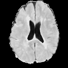
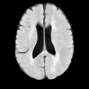
High-resolution image generation with VAEs is a topic of increasing interest [42] due to VAEs, in general, being easier to train than GANs. In our work, we introduce a novel means of generating high-resolution images with a VAE by adding a hierarchical binary latent space $\mathbf{z}_{0}$ and $\mathbf{z}_{1}$—in addition to the normal latent space $\mathbf{z}_{2}$—that preserves structural information of the input image without making the VAE an identity transformation. This latent space was inspired by the $\beta$ latent space of Dewey et al. [10]. We, however, use a hierarchy of latent spaces and use a KL term on the binary latent space that isn’t present in their work. A graphical representation of the VAE architecture is shown in Fig. 1. A non-counterfactual, unconditional sample from the SCM with our VAE is shown in Fig. 2.

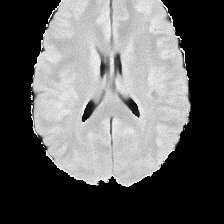
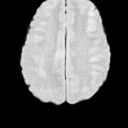
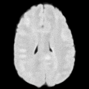
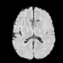
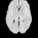
The binary latent space consists of a straight-through relaxed Bernoulli distribution using the Gumbel reparameterization [16] on two levels of the feature space. (The locations of which can be seen in Fig. 1 in the light blue lines.) The larger image-dimension binary latent space $\mathbf{z}_{0}$ is $N\times 64\times 64$ dimensions and the smaller image-dimension binary latent space $\mathbf{z}_{1}$ is $M\times 16\times 16$ dimension, where $M,N\in\mathbb{N}$ are experiment-specific parameters. The prior parameter for the Bernoulli distribution for both levels is set to 0.5; the recognition model (encoder) balances minimizing the KL divergence of the latent space (i.e., pushing the predicted probability to 0.5) and reconstructing the image—similar to the standard VAE framework with only a normal prior. A sample of $\mathbf{z}_{0}$ is shown in Fig. 3. As can be seen, the binary latent space captures a rough outline of the structure of the FLAIR image. It does so without passing so much information to the generative model (decoder) that it is unable to learn features of the data.

As can be seen in Fig. 3, the binary latent spaces are very noisy; this encourages the network to use the entire hierarchy of latent spaces. An analogy for why this is the case can be found in Cover and Thomas (Ch. 9) [8]. They discuss communication over multiple parallel noisy channels. The optimal configuration for maximal information transmission over parallel noisy channels is to use the channels according to the noise level of each channel (e.g., the variance of the noise). We hypothesize that the VAE learns a similar configuration based on the reliability of information transmission through the binary latent space.

We used a conditional VAE, conditioned on $\mathbf{c}=(n,b,v,l)^{\top}$, where $n$ is the slice number, $b$ is the brain volume, $v$ is ventricle volume, and $l$ is lesion volume. We concatenate $\mathbf{c}$ in the normal latent space $\mathbf{z}_{2}$, to make $\mathbf{z}_{c}=[\mathbf{z}_{2},\mathbf{c}]$, which is then input to the lowest level of the generative model. Additionally, to condition on $\mathbf{c}$ when also using binary latent spaces, we used squeeze-and-excite (channel-wise) attention [14] on the convolutional layers indicated with orange arrows in the generative model shown in Fig. 1, where the input to the squeeze-and-excite layers is $\mathbf{c}$.

Figure 2: Samples from the generative model: The above six images were generated by (unconditionally) ancestrally sampling the generative model trained on $128\times 128$ images. The varying location is due to training with random crops.

Figure 3: Binary latent space: Visualization of one channel of the binary latent space early in training (later in training it is harder to discern structure).

The generative model outputs image-sized location and scale parameters of a Laplace distribution. For simplicity, we assume pixels are independent so the location and scale images are the same size as the image. The Laplace distribution was used instead of a Gaussian because the $L_{1}$ loss has been noted to be preferable over MSE for image-related regression tasks [18] and we noticed a qualitative improvement in the predicted counterfactual images.

Training this VAE involves several tricks to stabilize training. We trained the model for 2000 epochs. We used a one-cycle learning rate schedule [37] with the Adam optimizer [19] starting at $2\times 10^{-5}$, increasing to $5\times 10^{-4}$ for the first 10% of training epochs, and decaying to $5\times 10^{-8}$. We also used a schedule for a scaling parameter $\lambda_{i}$ on the KL divergence terms as discussed in Sønderby et al. [38]; specifically, we started the KL divergence scaling parameter for the normal distribution $\lambda_{2}$ at 0 and linearly increased it to a maximum of 1 in 600 epochs. For the binary latent space KL terms $\lambda_{1}$ and $\lambda_{0}$, we started the scaling parameter at a small value and linearly increased them to different levels for the smaller and larger latent spaces; these settings are experiment-specific. We used weight normalization [34] on all convolutional layers. We also clipped the norm of the gradients at a norm of 100. Finally, we used one inverse autoregressive affine normalizing flow on the posterior, as discussed by Kingma et al. [20].

3.3 Learning and inference in the SCM and VAE with a PPL

We used the Pyro probabilistic programming language (PPL) to implement the SCM. A PPL is a programming language with terms corresponding to sampling and conditioning. Pyro is a higher-order PPL built upon PyTorch [25]. See van de Meent et al. [22] for an overview of PPLs.

The functions $f_{i}\in mathbf{F}$, which take causal parents $\mathrm{pa}_{i}$ as input and outputs some variable $v_{i}\in\mathbf{V}$, are represented by normalizing flows (NFs) and neural networks. All $f_{i}$ in our SCM are linear rational spline NFs [11], except the functions for the image $f_{\mathbf{x}}$, biological sex $f_{s}$, and slice number $f_{n}$. The image function $f_{\mathbf{x}}$ is the generative model part of the VAE described in the previous section. Biological sex and slice number are directly sampled from their base distributions (Bernoulli and uniform, respectively). The base distributions for the NFs are normal distributions with the log of the empirical mean and variance of the training data as the location and scale parameters, respectively. The base distribution for biological sex is a Bernoulli distribution with parameter equal to the mean of data (0 for male, 1 for female). The base distribution for slice number is uniform from the minimum to the maximum slice number in the training set. During training, the hypernetworks associated with the NFs and VAE are jointly updated with backpropagation using the (negative) evidence lower bound as a loss function. During inference, the learned $\mathbf{F}$ are fixed. A counterfactual image is generated using the single-world intervention graph formalism [32].

4 Experiments

4.1 Data

We used a private dataset containing 77 subjects of both healthy control (HC) subjects and subjects with MS. We randomly split the data into training, validation, and testing. The training set consisted of 68 subjects where 38 were HC and 30 had MS (29 with had relapsing-remitting MS and 1 had secondary-progressive MS). The total number of unique scans in the training set was 171; 124 scans of MS and 47 HC. The validation set had 7 subjects with 4 HC and 3 MS; 16 total unique scans consisting of 5 HC and 11 MS. The test set had 2 subjects with 1 HC and 1 MS; 4 total unique scans consisting of 2 HC and 2 MS.

Each subject had both a $T_{1}$-w and a FLAIR image. The $T_{1}$-w and FLAIR images were bias field-corrected with N4 [41]. The $T_{1}$-w image was rigidly registered to the MNI ICBM152 brain atlas with ANTs [1]. The FLAIR image was super-resolved with SMORE [46] and then registered to the $T_{1}$-w image. The white matter mean was then normalized to 1.0, where the white matter was found using fuzzy c-means on the $T_{1}$-w image [31]. The brain volume was measured by scaling the number of voxels inside the brain mask, found with ROBEX [15], according to the digital resolution (0.8 mm³). The ventricle volume was similarly computed by segmenting the ventricles with the convolutional neural network of Shao et al. [35]. The lesion volume was measured by training the Tiramisu network described by Zhang et al. [45] on a private dataset. The ventricle segmentation occasionally segmented lesions as well as ventricles for subjects with MS; the lesion mask was used to remove voxels associated with lesions from the ventricle mask. Axial slices of each image were converted to PNGs by extracting three adjacent slices, clipping the intensity at the 99.5^th percentile, scaling the image to range between $[0,255]$, and converting the type of the slice array to an 8-bit unsigned integer. In all experiments, uniform random noise is added to discrete random variables per Theis et al. [40].

4.2 SCM for MS

$$\vbox{\hbox{ \leavevmode\hbox to139.48pt{\vbox to93.92pt{\pgfpicture\makeatletter\hbox{\hskip 12.14906pt\lower-80.44731pt\hbox to0.0pt{\pgfsys@beginscope\pgfsys@invoke{ }\definecolor{pgfstrokecolor}{rgb}{0,0,0}\pgfsys@color@rgb@stroke{0}{0}{0}\pgfsys@invoke{ }\pgfsys@color@rgb@fill{0}{0}{0}\pgfsys@invoke{ }\pgfsys@setlinewidth{0.4pt}\pgfsys@invoke{ }\nullfont\hbox to0.0pt{\pgfsys@beginscope\pgfsys@invoke{ }{{}} {{}}{{}} {{{}{}{{}}{}}}{{{}}}{{{{}}{{}}}}{{}}{{}}{{{ }}}\hbox{\hbox{\hbox{{\pgfsys@beginscope\pgfsys@invoke{ }{{}{{{}}}{{}}{}{}{}{}{}{}{}{}{}{\pgfsys@moveto{2.2629pt}{0.0pt}\pgfsys@curveto{2.2629pt}{1.24977pt}{1.24977pt}{2.2629pt}{0.0pt}{2.2629pt}\pgfsys@curveto{-1.24977pt}{2.2629pt}{-2.2629pt}{1.24977pt}{-2.2629pt}{0.0pt}\pgfsys@curveto{-2.2629pt}{-1.24977pt}{-1.24977pt}{-2.2629pt}{0.0pt}{-2.2629pt}\pgfsys@curveto{1.24977pt}{-2.2629pt}{2.2629pt}{-1.24977pt}{2.2629pt}{0.0pt}\pgfsys@closepath\pgfsys@moveto{0.0pt}{0.0pt}\pgfsys@fill\pgfsys@invoke{ } }{{{{}}\pgfsys@beginscope\pgfsys@invoke{ }\pgfsys@transformcm{0.8}{0.0}{0.0}{0.8}{0.0pt}{0.0pt}\pgfsys@invoke{ }\hbox{{\definecolor{pgfstrokecolor}{rgb}{0,0,0}\pgfsys@color@rgb@stroke{0}{0}{0}\pgfsys@invoke{ }\pgfsys@color@rgb@fill{0}{0}{0}\pgfsys@invoke{ }\hbox{} }}\pgfsys@invoke{\lxSVG@closescope }\pgfsys@endscope}}} \pgfsys@invoke{\lxSVG@closescope }\pgfsys@endscope}}}\hbox{{\pgfsys@beginscope\pgfsys@invoke{ }{{}{}{{ {}{}}}{ {}{}} {{}{{}}}{{}{}}{}{{}{}}{}{}{}{}{} { }{{{{}}\pgfsys@beginscope\pgfsys@invoke{ }\pgfsys@transformcm{0.8}{0.0}{0.0}{0.8}{-2.11435pt}{5.2493pt}\pgfsys@invoke{ }\hbox{{\definecolor{pgfstrokecolor}{rgb}{0,0,0}\pgfsys@color@rgb@stroke{0}{0}{0}\pgfsys@invoke{ }\pgfsys@color@rgb@fill{0}{0}{0}\pgfsys@invoke{ }\hbox{{$a$}} }}\pgfsys@invoke{\lxSVG@closescope }\pgfsys@endscope}}} \pgfsys@invoke{\lxSVG@closescope }\pgfsys@endscope}}} {{}}{{}} {{{}{}{{}}{}}}{{{}}}{{{{}}{{}}}}{{}}{{}}{{{ }}}\hbox{\hbox{\hbox{{\pgfsys@beginscope\pgfsys@invoke{ }{{}{{{}}}{{}}{}{}{}{}{}{}{}{}{}{\pgfsys@moveto{36.40633pt}{-17.07172pt}\pgfsys@curveto{36.40633pt}{-15.82195pt}{35.3932pt}{-14.80882pt}{34.14343pt}{-14.80882pt}\pgfsys@curveto{32.89366pt}{-14.80882pt}{31.88054pt}{-15.82195pt}{31.88054pt}{-17.07172pt}\pgfsys@curveto{31.88054pt}{-18.32149pt}{32.89366pt}{-19.33461pt}{34.14343pt}{-19.33461pt}\pgfsys@curveto{35.3932pt}{-19.33461pt}{36.40633pt}{-18.32149pt}{36.40633pt}{-17.07172pt}\pgfsys@closepath\pgfsys@moveto{34.14343pt}{-17.07172pt}\pgfsys@fill\pgfsys@invoke{ } }{{{{}}\pgfsys@beginscope\pgfsys@invoke{ }\pgfsys@transformcm{0.8}{0.0}{0.0}{0.8}{34.14343pt}{-17.07172pt}\pgfsys@invoke{ }\hbox{{\definecolor{pgfstrokecolor}{rgb}{0,0,0}\pgfsys@color@rgb@stroke{0}{0}{0}\pgfsys@invoke{ }\pgfsys@color@rgb@fill{0}{0}{0}\pgfsys@invoke{ }\hbox{} }}\pgfsys@invoke{\lxSVG@closescope }\pgfsys@endscope}}} \pgfsys@invoke{\lxSVG@closescope }\pgfsys@endscope}}}\hbox{{\pgfsys@beginscope\pgfsys@invoke{ }{{}{}{{ {}{}}}{ {}{}} {{}{{}}}{{}{}}{}{{}{}}{}{}{}{}{} { }{{{{}}\pgfsys@beginscope\pgfsys@invoke{ }\pgfsys@transformcm{0.8}{0.0}{0.0}{0.8}{32.26855pt}{-11.82246pt}\pgfsys@invoke{ }\hbox{{\definecolor{pgfstrokecolor}{rgb}{0,0,0}\pgfsys@color@rgb@stroke{0}{0}{0}\pgfsys@invoke{ }\pgfsys@color@rgb@fill{0}{0}{0}\pgfsys@invoke{ }\hbox{{$s$}} }}\pgfsys@invoke{\lxSVG@closescope }\pgfsys@endscope}}} \pgfsys@invoke{\lxSVG@closescope }\pgfsys@endscope}}} {{}}{{}} {{{}{}{{}}{}}}{{{}}}{{{{}}{{}}}}{{}}{{}}{{{ }}}\hbox{\hbox{\hbox{{\pgfsys@beginscope\pgfsys@invoke{ }{{}{{{}}}{{}}{}{}{}{}{}{}{}{}{}{\pgfsys@moveto{70.54977pt}{-25.03865pt}\pgfsys@curveto{70.54977pt}{-23.78888pt}{69.53665pt}{-22.77576pt}{68.28688pt}{-22.77576pt}\pgfsys@curveto{67.03711pt}{-22.77576pt}{66.02399pt}{-23.78888pt}{66.02399pt}{-25.03865pt}\pgfsys@curveto{66.02399pt}{-26.28842pt}{67.03711pt}{-27.30154pt}{68.28688pt}{-27.30154pt}\pgfsys@curveto{69.53665pt}{-27.30154pt}{70.54977pt}{-26.28842pt}{70.54977pt}{-25.03865pt}\pgfsys@closepath\pgfsys@moveto{68.28688pt}{-25.03865pt}\pgfsys@fill\pgfsys@invoke{ } }{{{{}}\pgfsys@beginscope\pgfsys@invoke{ }\pgfsys@transformcm{0.8}{0.0}{0.0}{0.8}{68.28688pt}{-25.03865pt}\pgfsys@invoke{ }\hbox{{\definecolor{pgfstrokecolor}{rgb}{0,0,0}\pgfsys@color@rgb@stroke{0}{0}{0}\pgfsys@invoke{ }\pgfsys@color@rgb@fill{0}{0}{0}\pgfsys@invoke{ }\hbox{} }}\pgfsys@invoke{\lxSVG@closescope }\pgfsys@endscope}}} \pgfsys@invoke{\lxSVG@closescope }\pgfsys@endscope}}}\hbox{{\pgfsys@beginscope\pgfsys@invoke{ }{{}{}{{ {}{}}}{ {}{}} {{}{{}}}{{}{}}{}{{}{}}{}{}{}{}{} { }{{{{}}\pgfsys@beginscope\pgfsys@invoke{ }\pgfsys@transformcm{0.8}{0.0}{0.0}{0.8}{74.33644pt}{-26.76096pt}\pgfsys@invoke{ }\hbox{{\definecolor{pgfstrokecolor}{rgb}{0,0,0}\pgfsys@color@rgb@stroke{0}{0}{0}\pgfsys@invoke{ }\pgfsys@color@rgb@fill{0}{0}{0}\pgfsys@invoke{ }\hbox{{$e$}} }}\pgfsys@invoke{\lxSVG@closescope }\pgfsys@endscope}}} \pgfsys@invoke{\lxSVG@closescope }\pgfsys@endscope}}} {{}}{{}} {{{}{}{{}}{}}}{{{}}}{{{{}}{{}}}}{{}}{{}}{{{ }}}\hbox{\hbox{\hbox{{\pgfsys@beginscope\pgfsys@invoke{ }{{}{{{}}}{{}}{}{}{}{}{}{}{}{}{}{\pgfsys@moveto{93.31206pt}{-68.28688pt}\pgfsys@curveto{93.31206pt}{-67.03711pt}{92.29893pt}{-66.02399pt}{91.04916pt}{-66.02399pt}\pgfsys@curveto{89.7994pt}{-66.02399pt}{88.78627pt}{-67.03711pt}{88.78627pt}{-68.28688pt}\pgfsys@curveto{88.78627pt}{-69.53665pt}{89.7994pt}{-70.54977pt}{91.04916pt}{-70.54977pt}\pgfsys@curveto{92.29893pt}{-70.54977pt}{93.31206pt}{-69.53665pt}{93.31206pt}{-68.28688pt}\pgfsys@closepath\pgfsys@moveto{91.04916pt}{-68.28688pt}\pgfsys@fill\pgfsys@invoke{ } }{{{{}}\pgfsys@beginscope\pgfsys@invoke{ }\pgfsys@transformcm{0.8}{0.0}{0.0}{0.8}{91.04916pt}{-68.28688pt}\pgfsys@invoke{ }\hbox{{\definecolor{pgfstrokecolor}{rgb}{0,0,0}\pgfsys@color@rgb@stroke{0}{0}{0}\pgfsys@invoke{ }\pgfsys@color@rgb@fill{0}{0}{0}\pgfsys@invoke{ }\hbox{} }}\pgfsys@invoke{\lxSVG@closescope }\pgfsys@endscope}}} \pgfsys@invoke{\lxSVG@closescope }\pgfsys@endscope}}}\hbox{{\pgfsys@beginscope\pgfsys@invoke{ }{{}{}{{ {}{}}}{ {}{}} {{}{{}}}{{}{}}{}{{}{}}{}{}{}{}{} { }{{{{}}\pgfsys@beginscope\pgfsys@invoke{ }\pgfsys@transformcm{0.8}{0.0}{0.0}{0.8}{88.93839pt}{-77.7809pt}\pgfsys@invoke{ }\hbox{{\definecolor{pgfstrokecolor}{rgb}{0,0,0}\pgfsys@color@rgb@stroke{0}{0}{0}\pgfsys@invoke{ }\pgfsys@color@rgb@fill{0}{0}{0}\pgfsys@invoke{ }\hbox{{$\mathbf{x}$}} }}\pgfsys@invoke{\lxSVG@closescope }\pgfsys@endscope}}} \pgfsys@invoke{\lxSVG@closescope }\pgfsys@endscope}}} {{}}{{}} {{{}{}{{}}{}}}{{{}}}{{{{}}{{}}}}{{}}{{}}{{{ }}}\hbox{\hbox{\hbox{{\pgfsys@beginscope\pgfsys@invoke{ }{{}{{{}}}{{}}{}{}{}{}{}{}{}{}{}{\pgfsys@moveto{116.07436pt}{-68.28688pt}\pgfsys@curveto{116.07436pt}{-67.03711pt}{115.06123pt}{-66.02399pt}{113.81146pt}{-66.02399pt}\pgfsys@curveto{112.56169pt}{-66.02399pt}{111.54857pt}{-67.03711pt}{111.54857pt}{-68.28688pt}\pgfsys@curveto{111.54857pt}{-69.53665pt}{112.56169pt}{-70.54977pt}{113.81146pt}{-70.54977pt}\pgfsys@curveto{115.06123pt}{-70.54977pt}{116.07436pt}{-69.53665pt}{116.07436pt}{-68.28688pt}\pgfsys@closepath\pgfsys@moveto{113.81146pt}{-68.28688pt}\pgfsys@fill\pgfsys@invoke{ } }{{{{}}\pgfsys@beginscope\pgfsys@invoke{ }\pgfsys@transformcm{0.8}{0.0}{0.0}{0.8}{113.81146pt}{-68.28688pt}\pgfsys@invoke{ }\hbox{{\definecolor{pgfstrokecolor}{rgb}{0,0,0}\pgfsys@color@rgb@stroke{0}{0}{0}\pgfsys@invoke{ }\pgfsys@color@rgb@fill{0}{0}{0}\pgfsys@invoke{ }\hbox{} }}\pgfsys@invoke{\lxSVG@closescope }\pgfsys@endscope}}} \pgfsys@invoke{\lxSVG@closescope }\pgfsys@endscope}}}\hbox{{\pgfsys@beginscope\pgfsys@invoke{ }{{}{}{{ {}{}}}{ {}{}} {{}{{}}}{{}{}}{}{{}{}}{}{}{}{}{} { }{{{{}}\pgfsys@beginscope\pgfsys@invoke{ }\pgfsys@transformcm{0.8}{0.0}{0.0}{0.8}{119.86119pt}{-70.00934pt}\pgfsys@invoke{ }\hbox{{\definecolor{pgfstrokecolor}{rgb}{0,0,0}\pgfsys@color@rgb@stroke{0}{0}{0}\pgfsys@invoke{ }\pgfsys@color@rgb@fill{0}{0}{0}\pgfsys@invoke{ }\hbox{{$n$}} }}\pgfsys@invoke{\lxSVG@closescope }\pgfsys@endscope}}} \pgfsys@invoke{\lxSVG@closescope }\pgfsys@endscope}}} {{}}{{}} {{{}{}{{}}{}}}{{{}}}{{{{}}{{}}}}{{}}{{}}{{{ }}}\hbox{\hbox{\hbox{{\pgfsys@beginscope\pgfsys@invoke{ }{{}{{{}}}{{}}{}{}{}{}{}{}{}{}{}{\pgfsys@moveto{93.31206pt}{-45.52458pt}\pgfsys@curveto{93.31206pt}{-44.27481pt}{92.29893pt}{-43.26169pt}{91.04916pt}{-43.26169pt}\pgfsys@curveto{89.7994pt}{-43.26169pt}{88.78627pt}{-44.27481pt}{88.78627pt}{-45.52458pt}\pgfsys@curveto{88.78627pt}{-46.77435pt}{89.7994pt}{-47.78748pt}{91.04916pt}{-47.78748pt}\pgfsys@curveto{92.29893pt}{-47.78748pt}{93.31206pt}{-46.77435pt}{93.31206pt}{-45.52458pt}\pgfsys@closepath\pgfsys@moveto{91.04916pt}{-45.52458pt}\pgfsys@fill\pgfsys@invoke{ } }{{{{}}\pgfsys@beginscope\pgfsys@invoke{ }\pgfsys@transformcm{0.8}{0.0}{0.0}{0.8}{91.04916pt}{-45.52458pt}\pgfsys@invoke{ }\hbox{{\definecolor{pgfstrokecolor}{rgb}{0,0,0}\pgfsys@color@rgb@stroke{0}{0}{0}\pgfsys@invoke{ }\pgfsys@color@rgb@fill{0}{0}{0}\pgfsys@invoke{ }\hbox{} }}\pgfsys@invoke{\lxSVG@closescope }\pgfsys@endscope}}} \pgfsys@invoke{\lxSVG@closescope }\pgfsys@endscope}}}\hbox{{\pgfsys@beginscope\pgfsys@invoke{ }{{}{}{{ {}{}}}{ {}{}} {{}{{}}}{{}{}}{}{{}{}}{}{}{}{}{} { }{{{{}}\pgfsys@beginscope\pgfsys@invoke{ }\pgfsys@transformcm{0.8}{0.0}{0.0}{0.8}{97.09882pt}{-48.3025pt}\pgfsys@invoke{ }\hbox{{\definecolor{pgfstrokecolor}{rgb}{0,0,0}\pgfsys@color@rgb@stroke{0}{0}{0}\pgfsys@invoke{ }\pgfsys@color@rgb@fill{0}{0}{0}\pgfsys@invoke{ }\hbox{{$l$}} }}\pgfsys@invoke{\lxSVG@closescope }\pgfsys@endscope}}} \pgfsys@invoke{\lxSVG@closescope }\pgfsys@endscope}}} {{}}{{}} {{{}{}{{}}{}}}{{{}}}{{{{}}{{}}}}{{}}{{}}{{{ }}}\hbox{\hbox{\hbox{{\pgfsys@beginscope\pgfsys@invoke{ }{{}{{{}}}{{}}{}{}{}{}{}{}{}{}{}{\pgfsys@moveto{93.31206pt}{0.0pt}\pgfsys@curveto{93.31206pt}{1.24977pt}{92.29893pt}{2.2629pt}{91.04916pt}{2.2629pt}\pgfsys@curveto{89.7994pt}{2.2629pt}{88.78627pt}{1.24977pt}{88.78627pt}{0.0pt}\pgfsys@curveto{88.78627pt}{-1.24977pt}{89.7994pt}{-2.2629pt}{91.04916pt}{-2.2629pt}\pgfsys@curveto{92.29893pt}{-2.2629pt}{93.31206pt}{-1.24977pt}{93.31206pt}{0.0pt}\pgfsys@closepath\pgfsys@moveto{91.04916pt}{0.0pt}\pgfsys@fill\pgfsys@invoke{ } }{{{{}}\pgfsys@beginscope\pgfsys@invoke{ }\pgfsys@transformcm{0.8}{0.0}{0.0}{0.8}{91.04916pt}{0.0pt}\pgfsys@invoke{ }\hbox{{\definecolor{pgfstrokecolor}{rgb}{0,0,0}\pgfsys@color@rgb@stroke{0}{0}{0}\pgfsys@invoke{ }\pgfsys@color@rgb@fill{0}{0}{0}\pgfsys@invoke{ }\hbox{} }}\pgfsys@invoke{\lxSVG@closescope }\pgfsys@endscope}}} \pgfsys@invoke{\lxSVG@closescope }\pgfsys@endscope}}}\hbox{{\pgfsys@beginscope\pgfsys@invoke{ }{{}{}{{ {}{}}}{ {}{}} {{}{{}}}{{}{}}{}{{}{}}{}{}{}{}{} { }{{{{}}\pgfsys@beginscope\pgfsys@invoke{ }\pgfsys@transformcm{0.8}{0.0}{0.0}{0.8}{88.96756pt}{5.2493pt}\pgfsys@invoke{ }\hbox{{\definecolor{pgfstrokecolor}{rgb}{0,0,0}\pgfsys@color@rgb@stroke{0}{0}{0}\pgfsys@invoke{ }\pgfsys@color@rgb@fill{0}{0}{0}\pgfsys@invoke{ }\hbox{{$d$}} }}\pgfsys@invoke{\lxSVG@closescope }\pgfsys@endscope}}} \pgfsys@invoke{\lxSVG@closescope }\pgfsys@endscope}}} {{}}{{}} {{{}{}{{}}{}}}{{{}}}{{{{}}{{}}}}{{}}{{}}{{{ }}}\hbox{\hbox{\hbox{{\pgfsys@beginscope\pgfsys@invoke{ }{{}{{{}}}{{}}{}{}{}{}{}{}{}{}{}{\pgfsys@moveto{2.2629pt}{-68.28688pt}\pgfsys@curveto{2.2629pt}{-67.03711pt}{1.24977pt}{-66.02399pt}{0.0pt}{-66.02399pt}\pgfsys@curveto{-1.24977pt}{-66.02399pt}{-2.2629pt}{-67.03711pt}{-2.2629pt}{-68.28688pt}\pgfsys@curveto{-2.2629pt}{-69.53665pt}{-1.24977pt}{-70.54977pt}{0.0pt}{-70.54977pt}\pgfsys@curveto{1.24977pt}{-70.54977pt}{2.2629pt}{-69.53665pt}{2.2629pt}{-68.28688pt}\pgfsys@closepath\pgfsys@moveto{0.0pt}{-68.28688pt}\pgfsys@fill\pgfsys@invoke{ } }{{{{}}\pgfsys@beginscope\pgfsys@invoke{ }\pgfsys@transformcm{0.8}{0.0}{0.0}{0.8}{0.0pt}{-68.28688pt}\pgfsys@invoke{ }\hbox{{\definecolor{pgfstrokecolor}{rgb}{0,0,0}\pgfsys@color@rgb@stroke{0}{0}{0}\pgfsys@invoke{ }\pgfsys@color@rgb@fill{0}{0}{0}\pgfsys@invoke{ }\hbox{} }}\pgfsys@invoke{\lxSVG@closescope }\pgfsys@endscope}}} \pgfsys@invoke{\lxSVG@closescope }\pgfsys@endscope}}}\hbox{{\pgfsys@beginscope\pgfsys@invoke{ }{{}{}{{{}{}}}{{}{}} {{}{{}}}{{}{}}{}{{}{}}{}{}{}{}{} { }{{{{}}\pgfsys@beginscope\pgfsys@invoke{ }\pgfsys@transformcm{0.8}{0.0}{0.0}{0.8}{-9.48265pt}{-71.0649pt}\pgfsys@invoke{ }\hbox{{\definecolor{pgfstrokecolor}{rgb}{0,0,0}\pgfsys@color@rgb@stroke{0}{0}{0}\pgfsys@invoke{ }\pgfsys@color@rgb@fill{0}{0}{0}\pgfsys@invoke{ }\hbox{{$b$}} }}\pgfsys@invoke{\lxSVG@closescope }\pgfsys@endscope}}} \pgfsys@invoke{\lxSVG@closescope }\pgfsys@endscope}}} {{}}{{}} {{{}{}{{}}{}}}{{{}}}{{{{}}{{}}}}{{}}{{}}{{{ }}}\hbox{\hbox{\hbox{{\pgfsys@beginscope\pgfsys@invoke{ }{{}{{{}}}{{}}{}{}{}{}{}{}{}{}{}{\pgfsys@moveto{36.40633pt}{-39.834pt}\pgfsys@curveto{36.40633pt}{-38.58423pt}{35.3932pt}{-37.5711pt}{34.14343pt}{-37.5711pt}\pgfsys@curveto{32.89366pt}{-37.5711pt}{31.88054pt}{-38.58423pt}{31.88054pt}{-39.834pt}\pgfsys@curveto{31.88054pt}{-41.08377pt}{32.89366pt}{-42.0969pt}{34.14343pt}{-42.0969pt}\pgfsys@curveto{35.3932pt}{-42.0969pt}{36.40633pt}{-41.08377pt}{36.40633pt}{-39.834pt}\pgfsys@closepath\pgfsys@moveto{34.14343pt}{-39.834pt}\pgfsys@fill\pgfsys@invoke{ } }{{{{}}\pgfsys@beginscope\pgfsys@invoke{ }\pgfsys@transformcm{0.8}{0.0}{0.0}{0.8}{34.14343pt}{-39.834pt}\pgfsys@invoke{ }\hbox{{\definecolor{pgfstrokecolor}{rgb}{0,0,0}\pgfsys@color@rgb@stroke{0}{0}{0}\pgfsys@invoke{ }\pgfsys@color@rgb@fill{0}{0}{0}\pgfsys@invoke{ }\hbox{} }}\pgfsys@invoke{\lxSVG@closescope }\pgfsys@endscope}}} \pgfsys@invoke{\lxSVG@closescope }\pgfsys@endscope}}}\hbox{{\pgfsys@beginscope\pgfsys@invoke{ }{{}{}{{{}{}}}{{}{}} {{}{{}}}{{}{}}{}{{}{}}{}{}{}{}{} { }{{{{}}\pgfsys@beginscope\pgfsys@invoke{ }\pgfsys@transformcm{0.8}{0.0}{0.0}{0.8}{23.92943pt}{-41.55635pt}\pgfsys@invoke{ }\hbox{{\definecolor{pgfstrokecolor}{rgb}{0,0,0}\pgfsys@color@rgb@stroke{0}{0}{0}\pgfsys@invoke{ }\pgfsys@color@rgb@fill{0}{0}{0}\pgfsys@invoke{ }\hbox{{$v$}} }}\pgfsys@invoke{\lxSVG@closescope }\pgfsys@endscope}}} \pgfsys@invoke{\lxSVG@closescope }\pgfsys@endscope}}} {{}}{}{{}} {{{{{}}{}{}{}{}{{}}}}}{}{{{{{}}{}{}{}{}{{}}}}}{{}}{}{}{}\pgfsys@beginscope\pgfsys@invoke{ }\pgfsys@setlinewidth{0.8pt}\pgfsys@invoke{ }{}{{ {\pgfsys@beginscope\pgfsys@setlinewidth{0.64pt}\pgfsys@setdash{}{0.0pt}\pgfsys@roundcap\pgfsys@roundjoin{} {}{}{} {}{}{} \pgfsys@moveto{-1.55997pt}{2.07996pt}\pgfsys@curveto{-1.42996pt}{1.29997pt}{0.0pt}{0.12999pt}{0.38998pt}{0.0pt}\pgfsys@curveto{0.0pt}{-0.12999pt}{-1.42996pt}{-1.29997pt}{-1.55997pt}{-2.07996pt}\pgfsys@stroke\pgfsys@endscope}} }{}{}{{}}\pgfsys@moveto{70.08806pt}{-26.65956pt}\pgfsys@lineto{88.72086pt}{-43.42896pt}\pgfsys@stroke\pgfsys@invoke{ }{{}{{}}{}{}{{}}{{{}}{{{}}{\pgfsys@beginscope\pgfsys@invoke{ }\pgfsys@transformcm{0.7433}{-0.66896}{0.66896}{0.7433}{88.72084pt}{-43.42894pt}\pgfsys@invoke{ }\pgfsys@invoke{ \lxSVG@closescope }\pgfsys@invoke{\lxSVG@closescope }\pgfsys@endscope}}{{}}}} \pgfsys@invoke{\lxSVG@closescope }\pgfsys@endscope{{}}{}{{}} {{{{{}}{}{}{}{}{{}}}}}{}{{{{{}}{}{}{}{}{{}}}}}{{}}{}{}{}\pgfsys@beginscope\pgfsys@invoke{ }\pgfsys@setlinewidth{0.8pt}\pgfsys@invoke{ }{}{}{}{}{{}}\pgfsys@moveto{2.4229pt}{0.0pt}\pgfsys@lineto{87.91658pt}{0.0pt}\pgfsys@stroke\pgfsys@invoke{ }{{}{{}}{}{}{{}}{{{}}{{{}}{\pgfsys@beginscope\pgfsys@invoke{ }\pgfsys@transformcm{1.0}{0.0}{0.0}{1.0}{87.91658pt}{0.0pt}\pgfsys@invoke{ }\pgfsys@invoke{ \lxSVG@closescope }\pgfsys@invoke{\lxSVG@closescope }\pgfsys@endscope}}{{}}}} \pgfsys@invoke{\lxSVG@closescope }\pgfsys@endscope{{}}{}{{}} {{{{{}}{}{}{}{}{{}}}}}{}{{{{{}}{}{}{}{}{{}}}}}{{}}{}{}{}\pgfsys@beginscope\pgfsys@invoke{ }\pgfsys@setlinewidth{0.8pt}\pgfsys@invoke{ }{}{}{}{}{{}}\pgfsys@moveto{89.41972pt}{-1.7928pt}\pgfsys@lineto{70.39456pt}{-22.72057pt}\pgfsys@stroke\pgfsys@invoke{ }{{}{{}}{}{}{{}}{{{}}{{{}}{\pgfsys@beginscope\pgfsys@invoke{ }\pgfsys@transformcm{-0.67267}{-0.73994}{0.73994}{-0.67267}{70.39458pt}{-22.72057pt}\pgfsys@invoke{ }\pgfsys@invoke{ \lxSVG@closescope }\pgfsys@invoke{\lxSVG@closescope }\pgfsys@endscope}}{{}}}} \pgfsys@invoke{\lxSVG@closescope }\pgfsys@endscope{{}}{}{{}} {{{{{}}{}{}{}{}{{}}}}}{}{{{{{}}{}{}{}{}{{}}}}}{{}}{}{}{}\pgfsys@beginscope\pgfsys@invoke{ }\pgfsys@setlinewidth{0.8pt}\pgfsys@invoke{ }{}{}{}{}{{}}\pgfsys@moveto{89.0646pt}{-1.38942pt}\pgfsys@lineto{36.7101pt}{-38.03757pt}\pgfsys@stroke\pgfsys@invoke{ }{{}{{}}{}{}{{}}{{{}}{{{}}{\pgfsys@beginscope\pgfsys@invoke{ }\pgfsys@transformcm{-0.81923}{-0.57346}{0.57346}{-0.81923}{36.71011pt}{-38.03755pt}\pgfsys@invoke{ }\pgfsys@invoke{ \lxSVG@closescope }\pgfsys@invoke{\lxSVG@closescope }\pgfsys@endscope}}{{}}}} \pgfsys@invoke{\lxSVG@closescope }\pgfsys@endscope{{}}{}{{}} {{{{{}}{}{}{}{}{{}}}}}{}{{{{{}}{}{}{}{}{{}}}}}{{}}{}{}{}\pgfsys@beginscope\pgfsys@invoke{ }\pgfsys@setlinewidth{0.8pt}\pgfsys@invoke{ }{}{}{}{}{{}}\pgfsys@moveto{91.04953pt}{-2.4229pt}\pgfsys@lineto{91.04953pt}{-42.39183pt}\pgfsys@stroke\pgfsys@invoke{ }{{}{{}}{}{}{{}}{{{}}{{{}}{\pgfsys@beginscope\pgfsys@invoke{ }\pgfsys@transformcm{0.0}{-1.0}{1.0}{0.0}{91.04953pt}{-42.39183pt}\pgfsys@invoke{ }\pgfsys@invoke{ \lxSVG@closescope }\pgfsys@invoke{\lxSVG@closescope }\pgfsys@endscope}}{{}}}} \pgfsys@invoke{\lxSVG@closescope }\pgfsys@endscope{{}}{}{{}} {{{{{}}{}{}{}{}{{}}}}}{}{{{{{}}{}{}{}{}{{}}}}}{{}}{}{}{}\pgfsys@beginscope\pgfsys@invoke{ }\pgfsys@setlinewidth{0.8pt}\pgfsys@invoke{ }{}{}{}{}{{}}\pgfsys@moveto{91.04953pt}{-47.94765pt}\pgfsys@lineto{91.04953pt}{-65.15422pt}\pgfsys@stroke\pgfsys@invoke{ }{{}{{}}{}{}{{}}{{{}}{{{}}{\pgfsys@beginscope\pgfsys@invoke{ }\pgfsys@transformcm{0.0}{-1.0}{1.0}{0.0}{91.04953pt}{-65.15422pt}\pgfsys@invoke{ }\pgfsys@invoke{ \lxSVG@closescope }\pgfsys@invoke{\lxSVG@closescope }\pgfsys@endscope}}{{}}}} \pgfsys@invoke{\lxSVG@closescope }\pgfsys@endscope{{}}{}{{}} {{{{{}}{}{}{}{}{{}}}}}{}{{{{{}}{}{}{}{}{{}}}}}{{}}{}{}{}\pgfsys@beginscope\pgfsys@invoke{ }\pgfsys@setlinewidth{0.8pt}\pgfsys@invoke{ }{}{}{}{}{{}}\pgfsys@moveto{36.46425pt}{-16.37555pt}\pgfsys@lineto{88.04874pt}{-0.9002pt}\pgfsys@stroke\pgfsys@invoke{ }{{}{{}}{}{}{{}}{{{}}{{{}}{\pgfsys@beginscope\pgfsys@invoke{ }\pgfsys@transformcm{0.95782}{0.28735}{-0.28735}{0.95782}{88.04872pt}{-0.90022pt}\pgfsys@invoke{ }\pgfsys@invoke{ \lxSVG@closescope }\pgfsys@invoke{\lxSVG@closescope }\pgfsys@endscope}}{{}}}} \pgfsys@invoke{\lxSVG@closescope }\pgfsys@endscope{{}}{}{{}} {{{{{}}{}{}{}{}{{}}}}}{}{{{{{}}{}{}{}{}{{}}}}}{{}}{}{}{}\pgfsys@beginscope\pgfsys@invoke{ }\pgfsys@setlinewidth{0.8pt}\pgfsys@invoke{ }{}{}{}{}{{}}\pgfsys@moveto{1.8613pt}{-66.73604pt}\pgfsys@lineto{31.73682pt}{-41.83977pt}\pgfsys@stroke\pgfsys@invoke{ }{{}{{}}{}{}{{}}{{{}}{{{}}{\pgfsys@beginscope\pgfsys@invoke{ }\pgfsys@transformcm{0.76822}{0.64018}{-0.64018}{0.76822}{31.7368pt}{-41.83978pt}\pgfsys@invoke{ }\pgfsys@invoke{ \lxSVG@closescope }\pgfsys@invoke{\lxSVG@closescope }\pgfsys@endscope}}{{}}}} \pgfsys@invoke{\lxSVG@closescope }\pgfsys@endscope{{}}{}{{}} {{{{{}}{}{}{}{}{{}}}}}{}{{{{{}}{}{}{}{}{{}}}}}{{}}{}{}{}\pgfsys@beginscope\pgfsys@invoke{ }\pgfsys@setlinewidth{0.8pt}\pgfsys@invoke{ }{}{}{}{}{{}}\pgfsys@moveto{1.57678pt}{-1.8396pt}\pgfsys@lineto{32.10472pt}{-37.45546pt}\pgfsys@stroke\pgfsys@invoke{ }{{}{{}}{}{}{{}}{{{}}{{{}}{\pgfsys@beginscope\pgfsys@invoke{ }\pgfsys@transformcm{0.65079}{-0.75926}{0.75926}{0.65079}{32.1047pt}{-37.45546pt}\pgfsys@invoke{ }\pgfsys@invoke{ \lxSVG@closescope }\pgfsys@invoke{\lxSVG@closescope }\pgfsys@endscope}}{{}}}} \pgfsys@invoke{\lxSVG@closescope }\pgfsys@endscope{{}}{}{{}} {{{{{}}{}{}{}{}{{}}}}}{}{{{{{}}{}{}{}{}{{}}}}}{{}}{}{}{}\pgfsys@beginscope\pgfsys@invoke{ }\pgfsys@setlinewidth{0.8pt}\pgfsys@invoke{ }{}{}{}{}{{}}\pgfsys@moveto{0.0pt}{-2.4229pt}\pgfsys@lineto{0.0pt}{-65.15422pt}\pgfsys@stroke\pgfsys@invoke{ }{{}{{}}{}{}{{}}{{{}}{{{}}{\pgfsys@beginscope\pgfsys@invoke{ }\pgfsys@transformcm{0.0}{-1.0}{1.0}{0.0}{0.0pt}{-65.15422pt}\pgfsys@invoke{ }\pgfsys@invoke{ \lxSVG@closescope }\pgfsys@invoke{\lxSVG@closescope }\pgfsys@endscope}}{{}}}} \pgfsys@invoke{\lxSVG@closescope }\pgfsys@endscope{{}}{}{{}} {{{{{}}{}{}{}{}{{}}}}}{}{{{{{}}{}{}{}{}{{}}}}}{{}}{}{}{}\pgfsys@beginscope\pgfsys@invoke{ }\pgfsys@setlinewidth{0.8pt}\pgfsys@invoke{ }{}{}{}{}{{}}\pgfsys@moveto{36.31064pt}{-40.91771pt}\pgfsys@lineto{88.24738pt}{-66.88611pt}\pgfsys@stroke\pgfsys@invoke{ }{{}{{}}{}{}{{}}{{{}}{{{}}{\pgfsys@beginscope\pgfsys@invoke{ }\pgfsys@transformcm{0.89442}{-0.4472}{0.4472}{0.89442}{88.24738pt}{-66.8861pt}\pgfsys@invoke{ }\pgfsys@invoke{ \lxSVG@closescope }\pgfsys@invoke{\lxSVG@closescope }\pgfsys@endscope}}{{}}}} \pgfsys@invoke{\lxSVG@closescope }\pgfsys@endscope{{}}{}{{}} {{{{{}}{}{}{}{}{{}}}}}{}{{{{{}}{}{}{}{}{{}}}}}{{}}{}{}{}\pgfsys@beginscope\pgfsys@invoke{ }\pgfsys@setlinewidth{0.8pt}\pgfsys@invoke{ }{}{}{}{}{{}}\pgfsys@moveto{2.4229pt}{-68.28712pt}\pgfsys@lineto{87.91658pt}{-68.28712pt}\pgfsys@stroke\pgfsys@invoke{ }{{}{{}}{}{}{{}}{{{}}{{{}}{\pgfsys@beginscope\pgfsys@invoke{ }\pgfsys@transformcm{1.0}{0.0}{0.0}{1.0}{87.91658pt}{-68.28712pt}\pgfsys@invoke{ }\pgfsys@invoke{ \lxSVG@closescope }\pgfsys@invoke{\lxSVG@closescope }\pgfsys@endscope}}{{}}}} \pgfsys@invoke{\lxSVG@closescope }\pgfsys@endscope{{}}{}{{}} {{{{{}}{}{}{}{}{{}}}}}{}{{{{{}}{}{}{}{}{{}}}}}{{}}{}{}{}\pgfsys@beginscope\pgfsys@invoke{ }\pgfsys@setlinewidth{0.8pt}\pgfsys@invoke{ }{}{}{}{}{{}}\pgfsys@moveto{111.38898pt}{-68.28716pt}\pgfsys@lineto{94.18242pt}{-68.28716pt}\pgfsys@stroke\pgfsys@invoke{ }{{}{{}}{}{}{{}}{{{}}{{{}}{\pgfsys@beginscope\pgfsys@invoke{ }\pgfsys@transformcm{-1.0}{0.0}{0.0}{-1.0}{94.18242pt}{-68.28716pt}\pgfsys@invoke{ }\pgfsys@invoke{ \lxSVG@closescope }\pgfsys@invoke{\lxSVG@closescope }\pgfsys@endscope}}{{}}}} \pgfsys@invoke{\lxSVG@closescope }\pgfsys@endscope{{}}{}{{}} {{{{{}}{}{}{}{}{{}}}}}{}{{{{{}}{}{}{}{}{{}}}}}{{}}{}{}{}\pgfsys@beginscope\pgfsys@invoke{ }\pgfsys@setlinewidth{0.8pt}\pgfsys@invoke{ }{}{}{}{}{{}}\pgfsys@moveto{32.79956pt}{-19.08774pt}\pgfsys@lineto{1.7378pt}{-65.6804pt}\pgfsys@stroke\pgfsys@invoke{ }{{}{{}}{}{}{{}}{{{}}{{{}}{\pgfsys@beginscope\pgfsys@invoke{ }\pgfsys@transformcm{-0.5547}{-0.83205}{0.83205}{-0.5547}{1.73781pt}{-65.68039pt}\pgfsys@invoke{ }\pgfsys@invoke{ \lxSVG@closescope }\pgfsys@invoke{\lxSVG@closescope }\pgfsys@endscope}}{{}}}} \pgfsys@invoke{\lxSVG@closescope }\pgfsys@endscope{{}}{}{{}} {{{{{}}{}{}{}{}{{}}}}}{}{{{{{}}{}{}{}{}{{}}}}}{{}}{}{}{}\pgfsys@beginscope\pgfsys@invoke{ }\pgfsys@setlinewidth{0.8pt}\pgfsys@invoke{ }{}{}{}{}{{}}\pgfsys@moveto{36.50307pt}{-17.62233pt}\pgfsys@lineto{65.23618pt}{-24.32686pt}\pgfsys@stroke\pgfsys@invoke{ }{{}{{}}{}{}{{}}{{{}}{{{}}{\pgfsys@beginscope\pgfsys@invoke{ }\pgfsys@transformcm{0.97385}{-0.22723}{0.22723}{0.97385}{65.23618pt}{-24.32684pt}\pgfsys@invoke{ }\pgfsys@invoke{ \lxSVG@closescope }\pgfsys@invoke{\lxSVG@closescope }\pgfsys@endscope}}{{}}}} \pgfsys@invoke{\lxSVG@closescope }\pgfsys@endscope{{}}{}{{}} {{{{{}}{}{}{}{}{{}}}}}{}{{{{{}}{}{}{}{}{{}}}}}{{}}{}{}{}\pgfsys@beginscope\pgfsys@invoke{ }\pgfsys@setlinewidth{0.8pt}\pgfsys@invoke{ }{}{}{}{}{{}}\pgfsys@moveto{36.55443pt}{-40.07523pt}\pgfsys@lineto{87.93213pt}{-45.21304pt}\pgfsys@stroke\pgfsys@invoke{ }{{}{{}}{}{}{{}}{{{}}{{{}}{\pgfsys@beginscope\pgfsys@invoke{ }\pgfsys@transformcm{0.99504}{-0.0995}{0.0995}{0.99504}{87.93213pt}{-45.21303pt}\pgfsys@invoke{ }\pgfsys@invoke{ \lxSVG@closescope }\pgfsys@invoke{\lxSVG@closescope }\pgfsys@endscope}}{{}}}} \pgfsys@invoke{\lxSVG@closescope }\pgfsys@endscope{{}}{}{{}} {{{{{}}{}{}{}{}{{}}}}}{}{{{{{}}{}{}{}{}{{}}}}}{{}}{}{}{}\pgfsys@beginscope\pgfsys@invoke{ }\pgfsys@setlinewidth{0.8pt}\pgfsys@invoke{ }{}{}{}{}{{}}\pgfsys@moveto{2.35054pt}{-67.69954pt}\pgfsys@lineto{88.01015pt}{-46.28458pt}\pgfsys@stroke\pgfsys@invoke{ }{{}{{}}{}{}{{}}{{{}}{{{}}{\pgfsys@beginscope\pgfsys@invoke{ }\pgfsys@transformcm{0.97014}{0.24254}{-0.24254}{0.97014}{88.01013pt}{-46.28458pt}\pgfsys@invoke{ }\pgfsys@invoke{ \lxSVG@closescope }\pgfsys@invoke{\lxSVG@closescope }\pgfsys@endscope}}{{}}}} \pgfsys@invoke{\lxSVG@closescope }\pgfsys@endscope \pgfsys@invoke{\lxSVG@closescope }\pgfsys@endscope{}{}{}\hss}\pgfsys@discardpath\pgfsys@invoke{\lxSVG@closescope }\pgfsys@endscope\hss}}\lxSVG@closescope\endpgfpicture}} }}\begin{aligned} s&=f_{s}(u_{s})&\qquad b&=f_{b}(a,s,u_{b})\\ n&=f_{n}(u_{n})&v&=f_{v}(a,b,u_{v})\\ a&=f_{a}(u_{a})&l&=f_{l}(d,e,v,l,u_{l})\\ d&=f_{d}(a,s,u_{d})&\mathbf{x}&=f_{\mathbf{x}}(b,v,l,n,\mathbf{u}_{\mathbf{x}})\\ e&=f_{e}(s,d,u_{e})\\ \end{aligned} a s e \mathbf{x} n l d b v a s e \mathbf{x} n l d b v$$

Figure 4: Proposed structural causal model: (Only $\mathbf{V}$ are shown in the graph.) $a$ is age, $d$ is the duration of MS symptoms, $l$ is the lesion volume of the subject, $n$ is the slice number, $\mathbf{x}$ is the image, $b$ is the brain volume, $s$ is biological sex, $e$ is the expanded disability severity score (EDSS), and $v$ is the ventricle volume. The right-hand side shows the functional relationships $\mathbf{F}$ associated with $\mathbf{V}$ and $\mathbf{U}$ of the SCM.

The SCM we use for all experiments is shown as a DAG in Fig. 4. Note that we only show the endogenous variables $\mathbf{V}$ in Fig. 4. The SCM can alternatively be represented as a system of equations relating $\mathbf{V}$ and $\mathbf{U}$ via the equations $\mathbf{F}$ as shown on the right-hand side of Fig. 4. The $u_{i}$ are the background variables associated with an endogenous variable $v_{i}$. Note that $\mathbf{u}_{\mathbf{x}}=(\mathbf{z}_{\mathbf{x}},\bm{\varepsilon}_{\mathbf{x}})$ where $\mathbf{z}_{\mathbf{x}}=(\mathbf{z}_{0},\mathbf{z}_{1},\mathbf{z}_{2})$ are the non-invertible latent space terms estimated with the recognition model of the VAE and $\bm{\varepsilon}_{\mathbf{x}}$ is the invertible term. The edges in this SCM were determined by starting from the SCM described in Pawlowski et al. [26], densely adding reasonable edges to the new variables ($d$, $e$, and $l$), and pruning the edges over many experiments based on the quality of the counterfactual images.

4.3 Small images, large range

Figure 5: Example counterfactual images: The first image is the original FLAIR image of a person with MS, the remaining images show an intervention on the patient info and the resulting counterfactual images. From left-to-right the interventions set the 1) lesion volume to 0 mL, 2) duration of symptoms to 0 years, 3) EDSS to 0, and 4) duration and EDSS to 0.

Figure 6: Example intervention on lesion volume: Another example intervention setting lesion volume to 0 mL on subject with a large lesion load (65 mL).

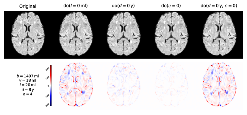
In this experiment, we randomly cropped the PNG images to $224\times 224$ pixels and downsampled the cropped patches to $128\times 128$ with linear interpolation. We used the middle 60 axial slices of the image volume as input for training, validation, and testing. The KL schedule for the binary latent space $\mathbf{z}_{0}$ and $\mathbf{z}_{1}$ both started at $\lambda_{0}=\lambda_{1}=1$ and ended at $\lambda_{0}=4.4$ and $\lambda_{1}=1.1$. We used a batch size of 342 for training. The latent space size parameters are $K=100$, $L=8192$, $M=4$, and $N=1$. A more detailed listing of all hyperparameters for this experiment can be found at the link in the footnote.

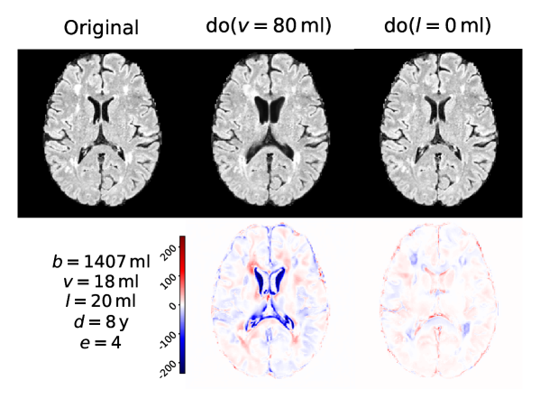
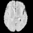
We show an example set of counterfactual images in Fig. 5. Another example counterfactual image is shown in Fig. 6 for a subject with a large lesion load. These counterfactuals are generated from subjects in the training set; the qualitative quality of counterfactuals on the validation and test set were worse. Recall, however, that these counterfactuals are not provided as examples for supervised learning of counterfactual prediction; predicting counterfactuals is an unsupervised problem. See the discussion section for additional details.

Figure 7: Lesion segmentation on original and counterfactual images: The left figure shows the histogram of segmented lesion volumes for original and counterfactual HC images, where lesion volume was set to 65 mL. The right figure shows a similar plot for original and counterfactual MS images, where lesion volume was set to 0 mL. The inset plots show the same data with the lesion volume for original on the left and counterfactual on the right.

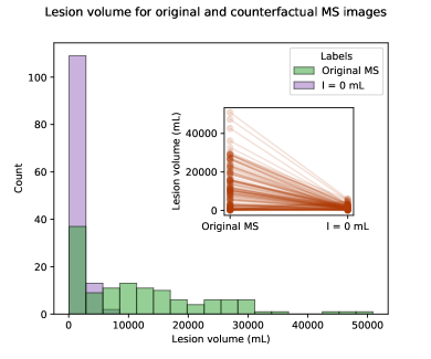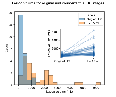
To quantify the effect of our counterfactuals on lesion volume, we used a lesion segmentation method on the original and counterfactual images. In the first experiment, we segmented HC images before and after an intervention setting lesion volume to 65 mL. The results for this experiment are summarized in the left-hand plot of Fig. 7. In the second experiment, we segmented MS images before and after an intervention setting lesion volume to 0 mL. The results are in the right-hand plot of the Fig. 7. Setting the lesion volume to 0 mL for people with MS consistently moves the lesion volume to near zero. But for HCs, setting lesion volume to 65 mL does not result in a consistent move to 65 mL. This is likely due to processing slices individually instead of as a volume. From the perspective of the SCM, only adding a few lesions in one slice is reasonable because the intervention lesion volume can be explained away by the presence of many lesions in other slices. This is a limitation of using two-dimensional images to generate counterfactuals with statistics computed from three-dimensional volumes.

4.4 Large images, small range

In this experiment, we cropped the images to $224\times 224$ and did not downsample the cropped patches. We used the middle 10 axial slices of the image volume as input for training, validation, and testing. The KL warm-up is similar to the previous experiment except for the KL schedule for $\mathbf{z}_{1}$ started at $\lambda_{1}=0.5$. We used a batch size of 128 for training. The latent space size parameters are $K=120$, $L=25088$, $M=8$, and $N=2$. An example intervention and samples from the generative model are shown in Fig. 8. A detailed listing of all hyperparameters for this experiment can be found at the link in the footnote

Samples

Figure 8: Large image counterfactuals and samples: The images on the left show an intervention setting 1) the ventricle volume to 80 mL, 2) the lesion volume to 0 mL. The two images on the right are samples from the generative model, similar to Fig. 2.

5 Discussion

In this work, we proposed an SCM to generate counterfactual images with application to MS. We showed that we can produce believable counterfactual images given a limited data set of healthy and MS subjects.

This work has many limitations. A noted problem with counterfactuals is that they are usually unverifiable. Counterfactuals imagine what some variable would look like in a parallel universe where all but the intervened on variables and their descendants were the same. Since we cannot validate our counterfactual images in a meaningful way, they should not be directly used for diagnosis or prognosis. The tools of causal inference, however, give researchers better ways to control for known confounders. As a result, the SCM framework can be potentially improve the performance of and trust in a machine learning system, e.g., in a harmonization or synthesis method.

Another limitation is that our model created poor counterfactual images for images outside the training set. However, causal inference is usually about retrospective analysis; generalization to new samples is not a requirement of a successful causal model. A statistical learning view of ML is that the aim of a predictor is to minimize the loss function under the true data distribution (i.e., the risk). Causal inference, however, is concerned with estimating the causal effect of a change in a covariate. Regardless, optimal hyperparameters and more data would likely help the SCM work better on unseen data.

Alternatives to the VAE should be further investigated because the causal effect of variables on one another is likely unidentifiable in the presence of the latent variables $\mathbf{z}$; this means that the functions $f_{i}$ do not necessarily reflect the true causal effect for a change in the parents.

The proposed SCM is a launching point for further refinement. The model is flawed and almost certainly requires additional variables to properly control for all confounders. For example, the type of treatment used should be included as variables and would make for more interesting counterfactuals (e.g., “what would this patient’s lesion load be if they had received interferon beta instead of glatiramer acetate?”). The fact that we don’t use this variable in our model can only hamper its performance. Better accounting for the relevant variables will improve performance and make more reliable counterfactual images.

In spite of the limitations, our SCM framework provides a principled way to generate a variety of images of interest for various applications (e.g., pseudo-healthy image synthesis) and analysis (e.g., counterfactual analysis of the effect of a medicine on lesion load). Such a framework can augment normal scientific analysis by providing a principled basis on which to test the effect of interventions outside of an RCT, and the generated counterfactual images have the potential to improve the performance of image processing pipelines and precision medicine in general.

References

- [1] Avants, B.B., Tustison, N., Song, G.: Advanced normalization tools (ANTS). Insight J 2(365), 1–35 (2009)
- [2] Bingham, E., Chen, J.P., Jankowiak, M., Obermeyer, F., Pradhan, N., Karaletsos, T., Singh, R., Szerlip, P., Horsfall, P., Goodman, N.D.: Pyro: Deep universal probabilistic programming. The Journal of Machine Learning Research 20(1), 973–978 (2019)
- [3] Blei, D.M., Kucukelbir, A., McAuliffe, J.D.: Variational inference: A review for statisticians. Journal of the American Statistical Association 112(518), 859–877 (2017)
- [4] Bowles, C., Qin, C., Guerrero, R., Gunn, R., Hammers, A., Dickie, D.A., Hernández, M.V., Wardlaw, J., Rueckert, D.: Brain lesion segmentation through image synthesis and outlier detection. NeuroImage: Clinical 16, 643–658 (2017)
- [5] Castro, D.C., Walker, I., Glocker, B.: Causality matters in medical imaging. Nature Communications 11(1), 1–10 (2020)
- [6] Chen, X., Duan, Y., Houthooft, R., Schulman, J., Sutskever, I., Abbeel, P.: InfoGAN: interpretable representation learning by information maximizing generative adversarial nets. In: Proceedings of the 30th International Conference on Neural Information Processing Systems. pp. 2180–2188 (2016)
- [7] Cohen, J.P., Luck, M., Honari, S.: Distribution matching losses can hallucinate features in medical image translation. In: International conference on medical image computing and computer-assisted intervention. pp. 529–536. Springer (2018)
- [8] Cover, T.M., Thomas, J.A.: Elements of Information Theory. John Wiley & Sons (2012)
- [9] Daniusis, P., Janzing, D., Mooij, J., Zscheischler, J., Steudel, B., Zhang, K., Schölkopf, B.: Inferring deterministic causal relations. arXiv preprint arXiv:1203.3475 (2012)
- [10] Dewey, B.E., Zuo, L., Carass, A., He, Y., Liu, Y., Mowry, E.M., Newsome, S., Oh, J., Calabresi, P.A., Prince, J.L.: A Disentangled Latent Space for Cross-Site MRI Harmonization. In: International Conference on Medical Image Computing and Computer-Assisted Intervention. pp. 720–729. Springer (2020)
- [11] Dolatabadi, H.M., Erfani, S., Leckie, C.: Invertible generative modeling using linear rational splines. In: International Conference on Artificial Intelligence and Statistics. pp. 4236–4246. PMLR (2020)
- [12] Gershman, S., Goodman, N.: Amortized inference in probabilistic reasoning. In: Proceedings of the annual meeting of the cognitive science society. vol. 36 (2014)
- [13] Higgins, I., Matthey, L., Pal, A., Burgess, C., Glorot, X., Botvinick, M., Mohamed, S., Lerchner, A.: -VAE: Learning basic visual concepts with a constrained variational framework. In: ICLR: International Conference on Learning Representations (2017)
- [14] Hu, J., Shen, L., Sun, G.: Squeeze-and-excitation networks. In: Proceedings of the IEEE Conference on Computer Vision and Pattern Recognition. pp. 7132–7141 (2018)
- [15] Iglesias, J.E., Liu, C.Y., Thompson, P.M., Tu, Z.: Robust brain extraction across datasets and comparison with publicly available methods. IEEE Transactions on Medical Imaging 30(9), 1617–1634 (2011)
- [16] Jang, E., Gu, S., Poole, B.: Categorical reparameterization with gumbel-softmax. In: International Conference on Learning Representations (2017)
- [17] Jordan, M.I., Ghahramani, Z., Jaakkola, T.S., Saul, L.K.: An introduction to variational methods for graphical models. Machine Learning 37(2), 183–233 (1999)
- [18] Kendall, A., Gal, Y.: What uncertainties do we need in bayesian deep learning for computer vision? In: Advances in neural information processing systems. pp. 5574–5584 (2017)
- [19] Kingma, D.P., Ba, J.L.: Adam: A method for stochastic gradient descent. In: ICLR: International Conference on Learning Representations. pp. 1–15 (2015)
- [20] Kingma, D.P., Salimans, T., Jozefowicz, R., Chen, X., Sutskever, I., Welling, M.: Improved Variational Inference with Inverse Autoregressive Flow. Advances in Neural Information Processing Systems 29, 4743–4751 (2016)
- [21] Locatello, F., Bauer, S., Lucic, M., Raetsch, G., Gelly, S., Schölkopf, B., Bachem, O.: A sober look at the unsupervised learning of disentangled representations and their evaluation. Journal of Machine Learning Research 21(209), 1–62 (2020)
- [22] van de Meent, J.W., Paige, B., Yang, H., Wood, F.: An introduction to probabilistic programming. arXiv preprint arXiv:1809.10756 (2018)
- [23] Mollison, D., Sellar, R., Bastin, M., Mollison, D., Chandran, S., Wardlaw, J., Connick, P.: The clinico-radiological paradox of cognitive function and MRI burden of white matter lesions in people with multiple sclerosis: A systematic review and meta-analysis. PloS ONE 12(5), e0177727 (2017)
- [24] Morgan, S.L., Winship, C.: Counterfactuals and causal inference. Cambridge University Press (2015)
- [25] Paszke, A., Gross, S., Massa, F., Lerer, A., Bradbury, J., Chanan, G., Killeen, T., Lin, Z., Gimelshein, N., Antiga, L., et al.: PyTorch: An Imperative Style, High-Performance Deep Learning Library. Advances in Neural Information Processing Systems 32, 8026–8037 (2019)
- [26] Pawlowski, N., Castro, D.C., Glocker, B.: Deep structural causal models for tractable counterfactual inference. In: Advances in Neural Information Processing Systems (2020)
- [27] Pearl, J.: Causality. Cambridge university press (2009)
- [28] Peters, J., Janzing, D., Schölkopf, B.: Elements of causal inference. The MIT Press (2017)
- [29] Ravi, D., Alexander, D.C., Oxtoby, N.P., Initiative, A.D.N., et al.: Degenerative adversarial NeuroImage nets: generating images that mimic disease progression. In: International Conference on Medical Image Computing and Computer-Assisted Intervention. pp. 164–172. Springer (2019)
- [30] Reich, D.S., Lucchinetti, C.F., Calabresi, P.A.: Multiple sclerosis. New England Journal of Medicine 378(2), 169–180 (2018)
- [31] Reinhold, J.C., Dewey, B.E., Carass, A., Prince, J.L.: Evaluating the impact of intensity normalization on MR image synthesis. In: Medical Imaging 2019: Image Processing. vol. 10949, p. 109493H. International Society for Optics and Photonics (2019)
- [32] Richardson, T.S., Robins, J.M.: Single world intervention graphs (SWIGs): A unification of the counterfactual and graphical approaches to causality. Center for the Statistics and the Social Sciences, University of Washington Series. Working Paper 128(30), 2013 (2013)
- [33] Ritchie, D., Horsfall, P., Goodman, N.D.: Deep amortized inference for probabilistic programs. arXiv preprint arXiv:1610.05735 (2016)
- [34] Salimans, T., Kingma, D.P.: Weight normalization: a simple reparameterization to accelerate training of deep neural networks. In: Proceedings of the 30th International Conference on Neural Information Processing Systems. pp. 901–909 (2016)
- [35] Shao, M., Han, S., Carass, A., Li, X., Blitz, A.M., Shin, J., Prince, J.L., Ellingsen, L.M.: Brain ventricle parcellation using a deep neural network: Application to patients with ventriculomegaly. NeuroImage: Clinical 23, 101871 (2019)
- [36] Shpitser, I., Pearl, J.: Complete identification methods for the causal hierarchy. Journal of Machine Learning Research 9, 1941–1979 (2008)
- [37] Smith, L.N.: Cyclical learning rates for training neural networks. In: 2017 IEEE Winter Conference on Applications of Computer Vision (WACV). pp. 464–472. IEEE (2017)
- [38] Sønderby, C.K., Raiko, T., Maaløe, L., Sønderby, S.K., Winther, O.: Ladder variational autoencoders. In: Proceedings of the 30th International Conference on Neural Information Processing Systems. pp. 3745–3753 (2016)
- [39] Spirtes, P.: Introduction to causal inference. Journal of Machine Learning Research 11(5) (2010)
- [40] Theis, L., van den Oord, A., Bethge, M.: A note on the evaluation of generative models. In: ICLR: International Conference on Learning Representations. pp. 1–10 (2016)
- [41] Tustison, N.J., Avants, B.B., Cook, P.A., Zheng, Y., Egan, A., Yushkevich, P.A., Gee, J.C.: N4ITK: Improved N3 bias correction. IEEE Transactions on Medical Imaging 29(6), 1310–1320 (2010)
- [42] Vahdat, A., Kautz, J.: NVAE: A deep hierarchical variational autoencoder. Advances in Neural Information Processing Systems 33 (2020)
- [43] Xia, T., Chartsias, A., Tsaftaris, S.A.: Pseudo-healthy synthesis with pathology disentanglement and adversarial learning. Medical Image Analysis 64, 101719 (2020)
- [44] Zhang, H., Bakshi, R., Bagnato, F., Oguz, I.: Robust Multiple Sclerosis Lesion Inpainting with Edge Prior. In: International Workshop on Machine Learning in Medical Imaging. pp. 120–129. Springer (2020)
- [45] Zhang, H., Valcarcel, A.M., Bakshi, R., Chu, R., Bagnato, F., Shinohara, R.T., Hett, K., Oguz, I.: Multiple sclerosis lesion segmentation with Tiramisu and 2.5D stacked slices. In: International Conference on Medical Image Computing and Computer-Assisted Intervention. pp. 338–346. Springer (2019)
- [46] Zhao, C., Dewey, B.E., Pham, D.L., Calabresi, P.A., Reich, D.S., Prince, J.L.: SMORE: A Self-supervised Anti-aliasing and Super-resolution Algorithm for MRI Using Deep Learning. IEEE Transactions on Medical Imaging (2020)
- [47] Zhu, J.Y., Park, T., Isola, P., Efros, A.A.: Unpaired image-to-image translation using cycle-consistent adversarial networks. In: Proceedings of the IEEE International Conference on Computer Vision. pp. 2223–2232 (2017)