From classical to quantum walks with stochastic resetting on networks
Abstract
Random walks are fundamental models of stochastic processes with applications in various fields including physics, biology, and computer science. We study classical and quantum random walks under the influence of stochastic resetting on arbitrary networks. Based on the mathematical formalism of quantum stochastic walks, we provide a framework of classical and quantum walks whose evolution is determined by graph Laplacians. We study the influence of quantum effects on the stationary and long-time average probability distribution by interpolating between the classical and quantum regime. We compare our analytical results on stationary and long-time average probability distributions with numerical simulations on different networks, revealing differences in the way resets affect the sampling properties of classical and quantum walks.
I Introduction
Karl Pearson coined the term “random walk” in a short commentary article in 1905 Pearson (1905). In the same year Albert Einstein described the random movements of particles suspended in a fluid in terms of Brownian motion Einstein (1905); Kac (1947), illustrating the potential of stochastic descriptions to improve our understanding of physical processes.
Early versions of random walks were also applied to problems in probability theory Epstein (2012) or in materials science Flory and Volkenstein (1969); Rubinstein et al. (2003); Gujrati and Leonov (2010). Nowadays, applications of random walks are quite versatile and are used to describe stock-price fluctuations Mandelbrot (1999); Malkiel (1999), foraging animals Mårell et al. (2002); Bartumeus et al. (2005), efficient search algorithms Gkantsidis et al. (2004) such as the famous PageRank Page et al. (1999) or even opinion formation DeGroot (1974); Böttcher et al. (2020); Böttcher and Gersbach (2020). We could continue this list but instead refer the interested reader to Refs. Ben-Avraham and Havlin (2000); Noh and Rieger (2004); Masuda et al. (2017) for further information.
Naturally, the success of classical random walks (CRWs)

has stimulated intensive research on the implementation and possible applications of quantum versions of random walks. Such quantum walks (QWs) have been realized in various experimental setup, cf. Ryan et al. (2005); Karski et al. (2009); Schmitz et al. (2009); Zähringer et al. (2010); Bouwmeester et al. (1999); Do et al. (2005); Schreiber et al. (2010); Perets et al. (2008). Although single particle QWs are usually closely related to classical wave phenomena Knight et al. (2003), quantum extensions Watrous (2001) led to important advances such as the development of hybrid classical-quantum versions of the PageRank Sánchez-Burillo et al. (2012); Lecca and Re (2019), new classes of quantum algorithms Shenvi et al. (2003); Childs and Goldstone (2004); Tulsi (2008); Magniez et al. (2011), and important insights into the feasibility of quantum computations in terms of QWs Childs (2009).111Note that different formulations of QWs have been proposed, including coined QWs Aharonov et al. (1993, 2001), or the formalism developed by Szegedy Szegedy (2004). Connections between coined and Szegedy QWs have been established through staggered QWs Portugal (2016); Portugal et al. (2016). For an overview of QWs and search algorithms, see Ref. Portugal (2013) and for yet other formulations of QWs see Refs. Leung et al. (2010); Kollár et al. (2012); Chandrashekar and Busch (2014); Elster et al. (2015); Portugal (2016); Ghosal and Deb (2018).
To use general walks in optimization problems it may be advantageous to employ algorithms with stochastic resetting Evans and Majumdar (2011); Evans et al. (2020), since optimization strategies without reset may end up in regions far away from the actual solutions Luby et al. (1993); Montero et al. (2017). Stochastic resetting is relevant not only in the context of search strategies, but also useful to sample certain rare events in simulations Villen-Altamirano et al. (1991). Furthermore, stochastic resetting has been theoretically analyzed in a tilted Bose–Hubbard system Mukherjee et al. (2018) for which results have been shown to smoothly interpolate between results obtained from the diagonal ensemble (vanishing reset rate) and the quantum Zeno effect (large reset rate). In a very recent work Riascos et al. (2020), classical random walks with stochastic resetting were studied on networks. For Caley trees, it was found that a classical random walker with an optimized stochastic resetting protocol performs similarly well as optimal search strategies in finding a target node at a certain distance. In other networks, the performance of such optimized random-walk searches depends on the centrality of the node that is chosen as reset state Riascos et al. (2020).
Motivated by the success of random-walk-based search strategies with stochastic resetting Ham et al. (2013); Valdeolivas et al. (2019), we study stochastic quantum walks with resetting on networks. To do so, we introduce a framework for classical, quantum, and hybrid random walks with stochastic resetting on networks. Our approach enables us to (i) interpolate between the classical and quantum regimes of such walks and (ii) analyze the influence of classical processes that perturb QWs. We explicitly show how a hybrid classical-quantum walk can be defined as an open quantum system and how the quantum jump operators and dissipation rates are connected to the CRW Hamiltonian. From this formulation, we derive the node occupation statistics in the stationary state of classical and quantum walks with stochastic resetting. We complement these efforts with a detailed numerical analysis for which we unravel the quantum master equation as stochastic Schrödinger equation and derive the adequate quantum jump probabilities. All codes that we used in this work are made publicly available git (2020).
The paper is organized as follows. In Sec. II, we briefly review some key concepts from the study of complex networks that will be used in our further analysis. In Sec. III, we provide precise definitions of the CRWs and the QWs we consider and understand these walks as cornerstones for a linear interpolation scheme that allows us to add “classicality” to QWs and vice versa “quantumness” to CRWs. Our general formulation of classical, quantum, and hybrid classical-quantum walks on networks utilizes the theoretical framework of quantum stochastic walks Whitfield et al. (2010), which we adapt to account for stochastic resetting. We compare our analytical results with corresponding simulations on different networks in Secs. IV and V. In Sec. VI, we discuss our results and conclude.
II Network science concepts
A graph (i.e., a network) is an ordered pair of two sets where is the set of nodes and is the set of edges, respectively Newman (2018). We denote the number of nodes by (i.e., ). Throughout this paper, we consider undirected networks, meaning that all edges are bidirectional, with unweighted edges. In order to describe dynamics on such graphs, we introduce a Hilbert space structure in the standard way by assigning to each node a basis vector . These basis vectors are chosen to be orthonormal, i.e. . The adjacency matrix of a graph describes the connections of the graph. For undirected networks with unweighted edges, each matrix element is
| (1) |
The adjacency matrix is thus a symmetric binary matrix and can be written in Dirac notation as
| (2) |
The degree of node is defined as the sum over the respective row of the adjacency matrix (i.e., ) and counts the number of connections leading to (respectively away from) node .
A characteristic quantity for graphs is the degree distribution that indicates the frequency of nodes with a certain degree. It is defined as , where is the number of nodes of degree in . The degree matrix of is
| (3) |
is a diagonal matrix whose elements correspond to the degree of the respective node. The evolution of CRWs and QWs on a graph can be described by the graph Laplacian Faccin et al. (2013)
| (4) |
These theoretical tools suffice for the study of the types of random walks that we envision. We shall now specify the set of graphs that we use in the present work. While our analytic results can be applied to general graphs, we will focus on the following three different networks for explicit numerical verification of our results.
-
•
Erdős-Rényi: Two nodes are connected with probability , which is independent of all other connections. Erdős-Rényi graphs have a binomial degree distribution Newman (2018).
-
•
Barabási-Albert: A new node will be attached to existing nodes and the attachment probability is proportional to the number of edges of the existing nodes. Here is the initial number of nodes. This preferential-attachment process leads to a scale-free network with an algebraic degree distribution Albert and Barabási (2002).
-
•
Peer-to-peer (p2p-Gnutella08): Nodes in this empirical network correspond to computers in a file-sharing network Leskovec and Krevl (2014).
In Fig. 1 we show the degree distributions and exemplary realizations of these networks. Our choice of the outlined networks is motivated by their different connectivity patterns, which enable us to study how such differences affect the properties of CRWs and QWs.

III Quantum Stochastic Walks on networks
In this section, we shall specify the types of walks on graphs that we study in the present work. Our choice is not unique and we refer the reader to Refs. Böttcher and Herrmann (2020); Portugal (2013) for an overview of different realizations of CRWs and QWs. The walks that we study in this work are schematically summarized in Fig. 2.
We start by introducing CRWs (Sec. III.1) in terms of their probability distribution and QWs (Sec. III.2) in terms of the corresponding wave function. CRWs and (continuous) QWs are fundamentally different, as the latter obey unitary dynamics as long as the walker is not measured, whereas the former do not. It has been argued that the characteristics of both types of dynamics can be incorporated in the dissipative dynamics of the density matrix of a quantum system, resulting in quantum stochastic walks Whitfield et al. (2010). General quantum stochastic processes can be described by a Lindblad master equation for the reduced density matrix of a quantum system222Here, and we apply this convention throughout the paper. Breuer and Petruccione (2002); Schaller (2014)
| (5) |
Here, is the quantum Hamiltonian of the system describing the coherent part of the dynamics which accounts for wave-like phenomena such as superposition and interference to take place. are certain quantum jump operators, each of which introduces an incoherent stochastic process to the dynamics of the quantum system. Thus, the above Lindblad dynamics is suitable to describe the interplay between classical hopping and quantum coherent evolution Whitfield et al. (2010).
The generic solution of Eq. (5) with the initial density matrix can be written in terms of the time-independent superoperator as
| (6) |
In the following sections, we employ a set of rules Whitfield et al. (2010) to include CRWs as stochastic background to QWs and we shall see that each classically allowed transition will result in a dissipative contribution to the superoperator.
We proceed as follows. In Secs. III.1 and III.2, we specify the types of CRWs and QWs on networks that we study in this paper. These can be seen as cornerstones of the outlined theory. In Sec. III.3, we introduce an interpolation scheme between these cornerstones and, in this way, define a quantum-to-classical random walk (QCW).333We use the term “quantum-to-classical” random walk to indicate that we consider a subset of QSWs that interpolates between CRWs and QWs. Finally, in Sec. III.4, we introduce stochastic resetting by means of a suitable quantum jump process.
III.1 Classical random walks on networks
We describe the evolution of a CRW on a network in terms of the probabilities of observing a walker on node at time . These probabilities form a normalized probability vector
| (7) |
In the time interval , conservation of probability implies that the local probabilities can only flow in and out of nodes. In particular, if is small enough, the net-influx to node originates from the immediate neighborhood of node . The evolution of the probability is thus described by the following rate equation
| (8) | ||||
The first term on the right-hand-side corresponds to the outward flow from node to its surroundings and the second term describes the inflow to node . We may rewrite Eq. (8) in matrix form
| (9) | ||||
with the graph Laplacian and the degree matrix (see Eqs. (3) and (4)). In the limit , this rate equation becomes a master equation in differential form
| (10) |
Here, we introduced the classical Hamiltonian as generator of time translation of the probability distribution. Equation (10) is formally solved with the time evolution operator which allows us to write the probability distribution at time , that originated from an initial distribution , as
| (11) |
For connected networks, where one can reach any node from any other node, and sufficiently long times, the CRW approaches a stationary probability distribution such that . This allows us to fully determine the stationary probability distribution as444It is straightforward to check that is indeed the steady state by applying the classical Hamiltonian to Eq. (12).
| (12) |
In the following sections, we will compare CRWs and QWs in terms of the probability that any of the nodes with degree is occupied. Note that satisfies
| (13) |
whereas we have in the node-centered formulation of the occupation probability.
III.2 Quantum walks on networks
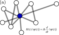
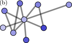
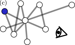
A quantum walker is described by its wave function rather than a probability distribution. The wave function propagates according to the Schrödinger equation
| (14) |
with some quantum Hamiltonian . This formulation of QWs is generally referred to as continuous time quantum walk Venegas-Andraca (2012). We note that a QW, as defined in Eq. (14), is not inherently stochastic since the Schrödinger equation itself is deterministic. Stochasticity in QWs rather stems from measurements that are applied to the quantum system and lead to a collapse of the wave-function Kollár et al. (2012) as illustrated in Fig. 3. In analogy to a CRW (see Eq. (11)), the quantum Hamiltonian generates a quantum-time-evolution operator
| (15) |
for a QW on . The choice of thus determines the behavior of the QW. We follow Ref. Faccin et al. (2013) and choose the symmetric and normalized graph Laplacian
| (16) |
as hermitian quantum Hamiltonian.555Note that the classical Hamiltonian is not necessarily Hermitian since in general (for a lattice we though have since ). QWs that are based on the Hamiltonian in Eq. (16) have the appealing property that the average probability to find the quantum walker on a certain node will be the same as in the classical case if the system is in the ground state (see Sec. III.1) Faccin et al. (2013); Biamonte et al. (2019).
In order to prepare the ground for more general quantum stochastic walks, we replace the wave function by the density matrix and the Schrödinger equation (see Eq. (14)) by the equivalent von-Neumann equation
| (17) |
This formulation is able to account for statistical mixtures of wave functions and can be easily extended to open quantum systems as needed for classical-quantum mixtures of random walks. For the QW that results from Eqs. (16) and (17), the long-time average probability of being on node is given by
| (18) |
Similar to the classical case, we denote by the probability that any node with degree is populated. As in Eq. (13), the probability satisfies
| (19) |
III.3 Quantum-to-classical stochastic walks
Having outlined frameworks for the treatment of CRWs and QWs on networks, we now proceed and introduce a generalized quantum stochastic walk that interpolates between these walks. We recall that any such walk is described by the Lindblad master equation (5) and introduce a dimensionless interpolation parameter in such a way that we recover the QW of Eq. (16) for . The choice
| (20) |
reduces the Lindblad master equation to the von-Neumann equation of the QW (see Eq. (17)), in the limit .
In order to also account for CRW dynamics, we need to choose specific dissipative processes by specifying the quantum jump operators . It has been shown that if the quantum jump operators satisfy the relation Whitfield et al. (2010)
| (21) | ||||
the classical processes induced by the classical Hamiltonian are encompassed in the dynamics of the generalized quantum system. In order to proceed, we choose the set of quantum jump operators666The explicit choice of the quantum jump operators is not unique.
| (22) |
induces jumps from node to node and satisfies
| (23) |
The parameters are the so-called damping constants. We use Eqs. (21) and (22) to determine the damping constants, viz.
| (24) |
It is important to distinguish between diagonal and off-diagonal contributions. Based on Eq. (10), it is clear that the off-diagonal elements of the classical Hamiltonian are negative, rendering the damping constants positive for . For , the entries of the classical Hamiltonian are equal to . Consequently, the parameter and thus
| (25) |
The full dynamics of a QCW is thus given by the Lindblad master equation
| (26) | ||||
Based on this expression, it is possible to explicitly show that this QCW recovers the CRW (see Eq. (10)) in the limit , see App. A for further details.
Despite the a priori phenomenological character of this approach to incorporate coherent and incoherent dynamical aspects, Eq. (26) can be considered as generic dynamics for a walker on a given graph structure. The parameter then indicates the competition between coherent and incoherent processes between neighboring nodes. This is most evident from an algorithmic point of view777See Sec. IV for a detailed description of the unfolding of the quantum master equation as a stochastic Schrödinger equation.: Imagine a discrete time step at the beginning of which a localized walker undergoes a unitary dynamics, meaning that the wave function spreads across the graph, see Fig. 3 (a) and (b). In the next time step, there is
-
•
a certain probability proportional to that an incoherent transition occurs from any node that the wave function occupies to a corresponding adjacent site.
-
•
a certain probability that the wave function spreads further in the neighborhood of already occupied sites.
In this manner, coherent and incoherent processes compete on the same graph in our hybrid quantum-to-classical walk formulation (26). Similar formulations have already proven to be of great use, e.g. in the design of quantum versions of the Page Rank Sánchez-Burillo et al. (2012), for graph isomorphism problems Bruderer and Plenio (2016), dissipative quantum computing algorithms Attal et al. (2012); Sinayskiy and Petruccione (2012), and decision-making Martínez-Martínez and Sánchez-Burillo (2016).
As the dissipator in Eq. (26) is well defined by the classical and quantum Hamiltonian and the parameter , we introduce the short-hand notation in terms of the superoperator
| (27) |
The QCW defined by Eq. (26) linearly interpolates between the CRWs and QWs that we defined in the preceding sections. This means that classical and quantum dynamics have been induced on the same network and that each link of this network is capable of hosting a classical and a quantum hopping process. One way to look at this is that finite thermal excitations in the system may introduce classical hopping on the quantum graph. This setup can be readily altered by, for instance, defining separate quantum and classical layers. We leave these directions for future works and focus instead on the dynamics induced by Eq. (26).
III.4 Reset quantum stochastic walks on networks
We describe stochastic resets by an additional dissipative contribution in the evolution of QCWs (see Eq. (26)) Rose et al. (2018). The modified Lindblad master equation including a reset process with a certain rate to the initial state reads (Rose et al., 2018, Eq. (59))
| (28) |
In the case of a pure reset state, the reset density matrix may be written as a projector . It turns out that the stationary state of the reset dynamics may be written explicitly in terms of left and right eigenmatrices and eigenvalues of the system without reset
| (29) |
The stationary state then reads Rose et al. (2018)
| (30) |
This holds for all and reset rates . In the case of a QW (), there is no stationary state without reset and Eq. (30) reduces to Rose et al. (2018)
| (31) |
where is the matrix of eigenvectors of the quantum Hamiltonian with and the elements of are
| (32) |
Equations (30) and (31) are remarkable since they express the stationary state of the reset dynamics in terms of the unperturbed system without reset (i.e., for ). This means that, e.g. for a QW where , the stationary state for is found analytically by diagonalizing the quantum Hamiltonian. Furthermore, for a general reset-QCW, the closed form allows us to determine the steady-state probability for the walker to be on node , viz.
| (33) | ||||
In the special case of a QW (), this formula reduces to Rose et al. (2018)
| (34) | ||||
where and are the eigenvalues and the eigenvectors of the quantum Hamiltonian . That is,
| (35) |
For a CRW (or QCW with ), it is also possible to directly determine the stationary probability distribution . In an infinitesimal time interval , the classical walk starts from its initial state with probability . The corresponding reset times are exponentially distributed with probability-density function . If the reset rate is finite (i.e., ), we find the corresponding stationary distribution (see App. B for further details)
| (36) | ||||
Note the similarity in the mathematical structure of Eqs. (34) and (36). One marked difference in is the appearance of product states that result from the mixing of wave-function components.
IV Numerical Recipes
In order to efficiently model classical and quantum random walks on large networks, we simulate the Lindblad master equation as piecewise deterministic process. The commonly used (but not unique) unfolding of the master equation (5) in terms of a stochastic Schrödinger equation reads Breuer and Petruccione (2002); Schaller (2014)
| (37) | ||||
Here is the wave function of a certain quantum trajectory and the Poisson increment describes a noisy contribution that is generated by the physical process belonging to the quantum jump operator . In each simulation step, the system either performs a time evolution according to the effective (non-hermitian) Hamiltonian
| (38) |
or otherwise an instantaneous quantum jump occurs. Quantum jumps satisfy
| (39) |
The probability that a jump process occurs in the time step is
| (40) |
The average over independently sampled quantum trajectories (or respectively the long-time limit of a single trajectory) allows us to determine the results of the Lindblad master equation.
IV.1 Stochastic Schrödinger equation for the reset dissipator

Here we discuss the numerical implementation of a quantum stochastic reset process for an otherwise unitary quantum walker. The inclusion of further dissipative processes is straightforward as the dissipative processes are additive in the Lindblad master equation (5). We shall exploit this fact in the next sections to write down the stochastic Schrödinger equation for a QCWs.
The quantum jump operators for the reset process presented in Sec. III.4 are Rose et al. (2018)
| (41) |
From Eq. (37) we obtain the corresponding stochastic Schrödinger equation
| (42) | ||||
with the quantum jump probability
| (43) |
We see that the quantum jump probability corresponds to the reset rate and does not depend on the current quantum state, as it should be for a stochastic reset process. Furthermore, the only difference to a brute-force reset is a global phase that keeps information about the pre-reset state. Since this phase is global, we neglect it in the remainder and write
| (44) |
This stochastic Schrödinger equation then yields the following simple stochastic rule for the time evolution of a unitary process with dissipative stochastic resets
| (45) | ||||
with a uniformly distributed random number and the Heaviside step function , which is 1 for and 0 otherwise. This description of quantum reset processes has been also used in previous studies Mukherjee et al. (2018); Rose et al. (2018).
In order to efficiently simulate the stochastic process induced by the reset (see Eq. (45)), we use a Crank-Nicholson scheme Askar and Cakmak (1978):
| (46) |
where the superscript indicates the time step. For reset-CRWs, we use Eq. (45) and replace by the probability vector and by the classical Hamiltonian . To numerically solve the evolution of CRWs, we use an Euler forward integration scheme.
IV.2 Classical-to-quantum walks
In Sec. III, we introduced the quantum jump operators
| (47) |
to include the CRW in a quantum process. The resulting master equation of the QCW is Eq. (26) and the corresponding unravelling (see Eq. (37)) can be written as
| (48) | ||||
with the Kronecker delta . The quantum jump probability belonging to this stochastic Schrödinger equation reads
| (49) |
where the first equality is the definition of the jump probability for the previously defined set of quantum jump operators and the second equality is a direct consequence of the specific shape of the classical Hamiltonian and the symmetry of the adjacency matrix. Note that the dissipative processes in Eq. (48) do not contain the interpolation parameter . Rather the jump probability in Eq. (49) is proportional to , rendering quantum jumps impossible in the unitary limit .
V Numerical Results on graphs
V.1 Classical and quantum walks with resetting
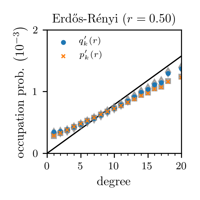
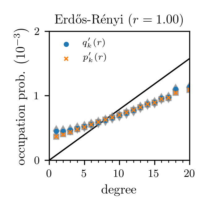
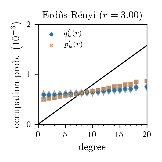
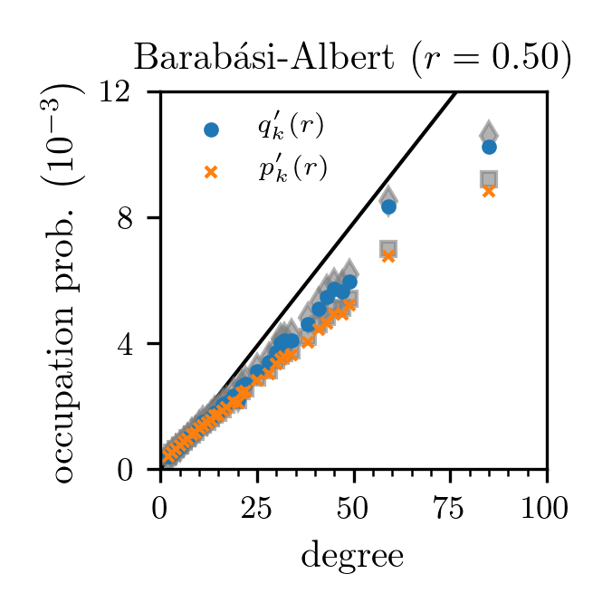
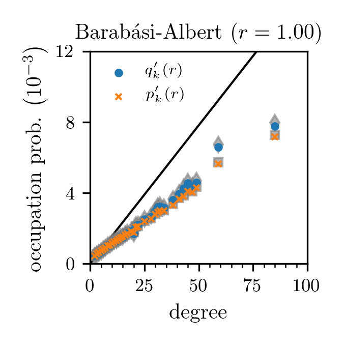
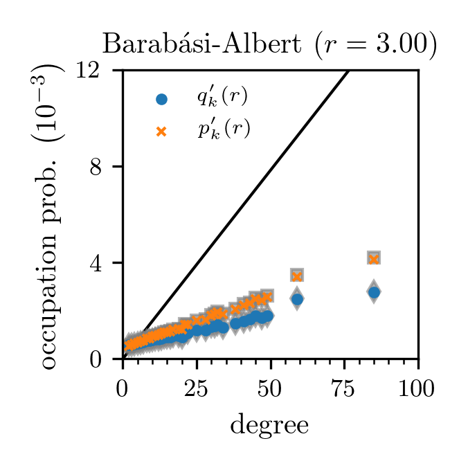
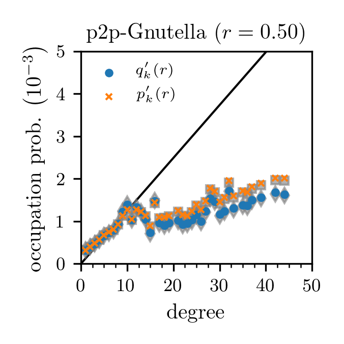
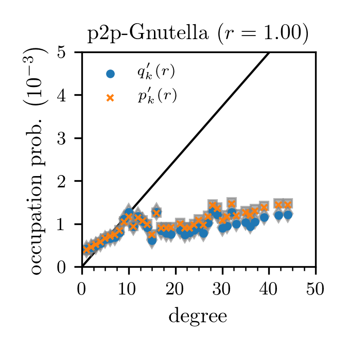
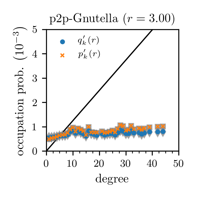
We now compare our analytical results of the stationary states of reset QCWs (see Eq. (33) and (34)) with the corresponding numerical solutions, given an underlying reset process with rate . In Fig. 4, we show the probabilities and that a node of degree is occupied by a classical and quantum random walker, respectively (see Eqs. (13) and (19)). We perform simulations on Erdős-Rényi, Barabási-Albert, and peer-to-peer networks (see Sec. II). The degree distribution of Erdős-Rényi networks is binomial whereas Barabási-Albert networks and the peer-to-peer networks exhibit broader degree distributions (see Fig. 1). As initial condition and reset state, we use a uniform distribution over all nodes. Thus, in the limit , the occupation probabilities satisfy for all degrees . In other words, for the chosen reset protocol, classical and quantum walks share the same node occupation probabilities as . Our results show that solutions of Eqs. (34) and (36) agree well with the numerically-obtained occupation probabilities on all networks for different reset rates .
We observe that the underlying network structure has a significant effect on how the occupation probabilities of the CRW and QW approach the limiting uniform distribution as becomes larger. In the Supplemental Material Wald and Böttcher (2020), we include an animation of the occupation-probability evolution for the three aforementioned networks. Quantum walks sample from the occupation probability distribution in a different way than CRWs. For an Erdős-Rényi network and a reset rate , low and high degree nodes are more likely to be sampled by a QW than by a CRW, which is different from what we observe for Barabási-Albert and peer-to-peer networks (see Fig. 4). For a given network, this difference in sampling can be controlled with the reset rate .
To determine the difference between and as a function of , we define the distance metric
| (50) |
where denotes the Euclidean norm. In Fig. 5, we show for the three networks of Sec. II. Numerical and analytical results are indicated by red and black solid lines, respectively. The distance between and is small, yet finite, for and vanishes as . Interestingly, we observe multiple inflection points in for the Erdős-Rényi and Barabási-Albert networks and a maximum distance at for the peer-to-peer and Erdős-Rényi networks. After the initial local minimum at , the distance between the classical and quantum occupation-probability distributions reaches a second pronounced local minimum at and for the Erdős-Rényi and Barabási-Albert networks, respectively. Each minimum corresponds to a cross-over of and . Based on the observed behavior of , , and , we conclude that classical and quantum occupation probabilities strongly depend on the underlying network structure and are not affected in the same way by changes of the reset rate . The initial increase of the distance with the reset rate seems to be universal throughout our results and may be explained with the initially strong impact of stochastic resetting on CRWs. While the long-time behavior of QWs is characterized by Eq. (18), CRWs have a unique stationary distribution that differs from our chosen reset state in heterogeneous networks. Therefore, the resetting mechanism introduces a strong competition between the reset state and the stationary state that strongly affects the node occupation properties of CRWs. Conversly, for large reset rates, the results in Fig. 4 and Wald and Böttcher (2020) show that QWs are closer to the uniform reset state for large reset rates. This can be qualitatively traced back to the strong mixing of the unitary dynamics: As the reset becomes the dominant contribution in the dynamics, mixing leads to a rather large overlap with the reset state and thus facilitates the relaxation into the reset state.
As described in Ref. Faccin et al. (2013), differences between the node occupation statistics of CRWs and QWs (without stochastic resetting, i.e., ) are largest on networks with a heterogeneous degree distribution (e.g., Barabási-Albert networks). As we show in Fig. 4, stochastic resetting can substantially increase these differences. For instance, in the considered Barabási-Albert network, the distance between CRWs and QWs is about 4–5 times larger for certain reset rates than .
V.2 Reset quantum-to-classical walks
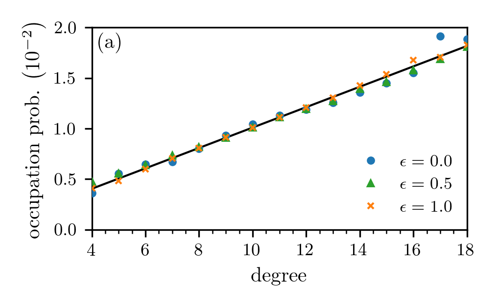
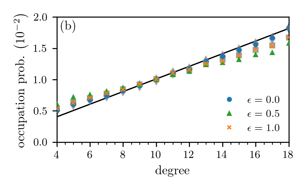
Figures 6 (a) and (b) show the occupation probability distribution of a QCW (see Eq. (48)) with and on an Erdős-Rényi network. Note that the limits and correspond to the purely quantum and classical case, respectively. For , we obtain a hybrid quantum-to-classical walk with yet different node-occupation statistics.
Our simulation results in Fig. 6 (a) confirm that the node occupation statistics of a QCW with and (orange crosses) agree with those of a CRW (black solid line). We also find that the analytical solutions (34) and (36) of the limiting cases (grey markers) agree with the corresponding simulations results for a reset rate of (see Fig. 6(b)). Interestingly, the hybrid quantum-classical walk with is affected more by the finite reset rate than its purely classical and quantum counterparts.
VI Discussion and Outlook
Random walks are important models of diffusive processes in many branches of science. In this work, we introduced a framework for the study of classical, quantum, and hybrid random walks with stochastic resetting on networks. We derived analytical solutions for the probability that a classical or quantum random walker occupies a certain node on a network. These analytical results, valid for general reset rates and network structures, are in perfect accordance with numerical solutions of the underlying master equations. Our results also revealed differences in the way classical and quantum walks with reset sample nodes with certain degrees. Both walks react differently to changes in the reset rate, which may be used as a control parameter to achieve desired node occupation (or sampling) statistics in quantum search and optimization algorithms Childs and Goldstone (2004); Douglas and Wang (2008); Chakraborty et al. (2016).
For the networks and uniform reset state that we studied in this paper, quantum walks are closer to the reset state than classical walks as the reset rate becomes large (see Fig. 4 and Wald and Böttcher (2020)). This behavior is linked to the unitary dynamics of QWs, which mixes quantum states (see Eq. (34)) and produces wave-function components that are close to the uniform reset state. Therefore, QWs reach such states “faster” (in the terms of a smaller reset rate) than classical walks. For large reset rates, the stationary distribution of CRWs is significantly altered from the one without resets. We thus find a competition between random-walk dynamics and reset dynamics, where both processes compete at different time scales.
In future work, our framework may be used to study how quantum walk search is affected by stochastic resetting as was done for classical walks in Ref. Riascos et al. (2020). Our framework is also directly applicable to compute classical, quantum, and hybrid random-walk-based centrality metrics on networks. In contrast to earlier studies Sánchez-Burillo et al. (2012); Rossi et al. (2014); Izaac et al. (2017), we also account for stochastic resetting, providing a possibility to reach desired node occupation statistics and design tailored centrality measures.
Other areas of application for resetting mechanisms include quantum feedback control Nelson et al. (2000); Eastman et al. (2017) and repeated measurements Evans et al. (2020). In these setups one repeatedly measures the quantum system and tailors the dynamics depending on the experimental outcome. Such formulations might be useful to impose constraints on the quantum system and in this manner induce non-trivial dynamical behavior on otherwise free quantum systems Maraga et al. (2015); Wald and Henkel (2016); Wald et al. (2018); Timpanaro et al. (2019); Wald et al. (2020); Halimeh and Maghrebi (2020).
While there has been rapid theoretical progress in the field of classical and quantum dynamics with stochastic resetting Evans et al. (2020), it will be important to also focus on experimental realizations of such processes in future studies and adapt theoretical models according to experimental protocols. As described in Ref. Evans et al. (2020), “in a theoretical model one often assumes instantaneous resetting which is impossible to achieve experimentally. Thus experimentalists need to devise different types of resetting protocols, which in turn pose interesting theoretical challenges.”
All codes are publicly available on GitHub git (2020).
Acknowledgments
We thank M Henkel, M Heyl, and F Semião for helpful comments. LB acknowledges financial support from the SNF Early Postdoc.Mobility fellowship on “Multispecies interacting stochastic systems in biology” and from the Army Research Office (W911NF-18-1-0345).
Appendix A Inclusion of CRW in QCW
In this appendix we show that the construction outlined in Sec. III.3 reduces to the CRW (see Eq. (10)) in the limit . This is done by evaluating the time evolution of the corresponding occupation probabilities . We utilize the Lindblad master equation (26) to derive the time evolution of the probabilities, viz.
| (51) | ||||
It is then clear that we can reduce the double sum to a single sum due to the Kronecker delta terms and we see that there are two distinct contributions, viz.
| (52) | ||||
The first term is already in the correct shape to reproduce the classical dynamics and solely the diagonal contributions are differ. We need to use the explicit form of the classical Hamiltonian, in particular that the diagonal elements are equal to in order to rewrite the second contribution. It is then straightforward to carry the calculation out as
| (53) | ||||
where we also used the symmetry of the adjacency matrix . This proves that the generated dynamics coincides with the stochastic dynamics defined in Eq. (10).
Appendix B Resolvent of infinitesimal generator
In this appendix, we illustrate the use of resolvents to formally solve differential equations. We consider the matrix differential equation
| (54) |
for the vector function and . We introduce the Laplace transform of as
| (55) |
Applying the Laplace transform to Eq. (54) yields
| (56) |
In this way we reduced the differential equation (54) to an algebraic equation
| (57) |
whose solution is readily found. The operator is called the resolvent of Pazy (2012). An integral representation of the resolvent is found by applying the Laplace transform directly to the solution of Eq. (54), we find
| (58) |
Combining Eqs. (56) and (58) yields
| (59) |
This identity is used in Eq. (36) in order to explicitly determine the stationary state of the CRW.
References
- Pearson (1905) K. Pearson, Nature 72, 342 (1905).
- Einstein (1905) A. Einstein, Annalen der Physik 322, 549 (1905).
- Kac (1947) M. Kac, The American Mathematical Monthly 54, 369 (1947).
- Epstein (2012) R. A. Epstein, The theory of gambling and statistical logic (Academic Press, 2012).
- Flory and Volkenstein (1969) P. J. Flory and M. Volkenstein, Biopolymers: Original Research on Biomolecules 8, 699 (1969).
- Rubinstein et al. (2003) M. Rubinstein, R. H. Colby, et al., Polymer physics, Vol. 23 (Oxford university press New York, 2003).
- Gujrati and Leonov (2010) P. D. Gujrati and A. I. Leonov, Modeling and simulation in polymers (John Wiley & Sons, 2010).
- Mandelbrot (1999) B. B. Mandelbrot, Scientific American 280, 70 (1999).
- Malkiel (1999) B. G. Malkiel, A random walk down Wall Street: including a life-cycle guide to personal investing (WW Norton & Company, 1999).
- Mårell et al. (2002) A. Mårell, J. P. Ball, and A. Hofgaard, Canadian Journal of Zoology 80, 854 (2002).
- Bartumeus et al. (2005) F. Bartumeus, M. G. E. da Luz, G. M. Viswanathan, and J. Catalan, Ecology 86, 3078 (2005).
- Gkantsidis et al. (2004) C. Gkantsidis, M. Mihail, and A. Saberi, in IEEE INFOCOM 2004, Vol. 1 (IEEE, 2004).
- Page et al. (1999) L. Page, S. Brin, R. Motwani, and T. Winograd, The pagerank citation ranking: Bringing order to the web., Tech. Rep. (Stanford InfoLab, 1999).
- DeGroot (1974) M. H. DeGroot, Journal of the American Statistical Association 69, 118 (1974).
- Böttcher et al. (2020) L. Böttcher, P. Montealegre, E. Goles, and H. Gersbach, Physica A: Statistical Mechanics and its Applications 545, 123713 (2020).
- Böttcher and Gersbach (2020) L. Böttcher and H. Gersbach, arXiv preprint arXiv:2001.05163 (2020).
- Ben-Avraham and Havlin (2000) D. Ben-Avraham and S. Havlin, Diffusion and reactions in fractals and disordered systems (Cambridge university press, 2000).
- Noh and Rieger (2004) J. D. Noh and H. Rieger, Physical Review Letters 92, 118701 (2004).
- Masuda et al. (2017) N. Masuda, M. A. Porter, and R. Lambiotte, Physics Reports 716, 1 (2017).
- Albert and Barabási (2002) R. Albert and A.-L. Barabási, Reviews of modern physics 74, 47 (2002).
- Leskovec and Krevl (2014) J. Leskovec and A. Krevl, “SNAP Datasets: Stanford large network dataset collection,” http://snap.stanford.edu/data (2014).
- Ryan et al. (2005) C. A. Ryan, M. Laforest, J. C. Boileau, and R. Laflamme, Phys. Rev. A 72, 062317 (2005).
- Karski et al. (2009) M. Karski, L. Förster, J.-M. Choi, A. Steffen, W. Alt, D. Meschede, and A. Widera, Science 325, 174 (2009).
- Schmitz et al. (2009) H. Schmitz, R. Matjeschk, C. Schneider, J. Glueckert, M. Enderlein, T. Huber, and T. Schaetz, Phys. Rev. Lett. 103, 090504 (2009).
- Zähringer et al. (2010) F. Zähringer, G. Kirchmair, R. Gerritsma, E. Solano, R. Blatt, and C. F. Roos, Phys. Rev. Lett. 104, 100503 (2010).
- Bouwmeester et al. (1999) D. Bouwmeester, I. Marzoli, G. P. Karman, W. Schleich, and J. P. Woerdman, Phys. Rev. A 61, 013410 (1999).
- Do et al. (2005) B. Do, M. L. Stohler, S. Balasubramanian, D. S. Elliott, C. Eash, E. Fischbach, M. A. Fischbach, A. Mills, and B. Zwickl, Journal of the Optical Society of America B 22, 499 (2005).
- Schreiber et al. (2010) A. Schreiber, K. N. Cassemiro, V. Potoček, A. Gábris, P. J. Mosley, E. Andersson, I. Jex, and C. Silberhorn, Phys. Rev. Lett. 104, 050502 (2010).
- Perets et al. (2008) H. B. Perets, Y. Lahini, F. Pozzi, M. Sorel, R. Morandotti, and Y. Silberberg, Phys. Rev. Lett. 100, 170506 (2008).
- Knight et al. (2003) P. L. Knight, E. Roldán, and J. E. Sipe, Phys. Rev. A 68, 020301 (2003).
- Watrous (2001) J. Watrous, Journal of computer and system sciences 62, 376 (2001).
- Sánchez-Burillo et al. (2012) E. Sánchez-Burillo, J. Duch, J. Gómez-Gardeñes, and D. Zueco, Scientific Reports 2 (2012), 10.1038/srep00605.
- Lecca and Re (2019) P. Lecca and A. Re, Theoretical Physics for Biological Systems (CRC Press, 2019).
- Shenvi et al. (2003) N. Shenvi, J. Kempe, and K. B. Whaley, Physical Review A 67, 052307 (2003).
- Childs and Goldstone (2004) A. M. Childs and J. Goldstone, Physical Review A 70, 022314 (2004).
- Tulsi (2008) A. Tulsi, Physical Review A 78, 012310 (2008).
- Magniez et al. (2011) F. Magniez, A. Nayak, J. Roland, and M. Santha, SIAM Journal on Computing 40, 142 (2011).
- Childs (2009) A. M. Childs, Physical Review Letters 102, 180501 (2009).
- Aharonov et al. (1993) Y. Aharonov, L. Davidovich, and N. Zagury, Physical Review A 48, 1687 (1993).
- Aharonov et al. (2001) D. Aharonov, A. Ambainis, J. Kempe, and U. Vazirani, in Proceedings of the thirty-third annual ACM symposium on Theory of computing (2001) pp. 50–59.
- Szegedy (2004) M. Szegedy, in 45th Annual IEEE symposium on foundations of computer science (IEEE, 2004) pp. 32–41.
- Portugal (2016) R. Portugal, Physical Review A 93, 062335 (2016).
- Portugal et al. (2016) R. Portugal, R. A. Santos, T. D. Fernandes, and D. N. Gonçalves, Quantum Information Processing 15, 85 (2016).
- Portugal (2013) R. Portugal, Quantum walks and search algorithms (Springer, 2013).
- Leung et al. (2010) G. Leung, P. Knott, J. Bailey, and V. Kendon, New Journal of Physics 12, 123018 (2010).
- Kollár et al. (2012) B. Kollár, T. Kiss, J. Novotnỳ, and I. Jex, Physical review letters 108, 230505 (2012).
- Chandrashekar and Busch (2014) C. Chandrashekar and T. Busch, Scientific reports 4, 6583 (2014).
- Elster et al. (2015) F. Elster, S. Barkhofen, T. Nitsche, J. Novotnỳ, A. Gábris, I. Jex, and C. Silberhorn, Scientific reports 5, 13495 (2015).
- Ghosal and Deb (2018) A. Ghosal and P. Deb, Physical Review A 98, 032104 (2018).
- Evans and Majumdar (2011) M. R. Evans and S. N. Majumdar, Phys. Rev. Lett. 106, 160601 (2011).
- Evans et al. (2020) M. R. Evans, S. N. Majumdar, and G. Schehr, Journal of Physics A: Mathematical and Theoretical 53, 193001 (2020).
- Luby et al. (1993) M. Luby, A. Sinclair, and D. Zuckerman, Information Processing Letters 47, 173 (1993).
- Montero et al. (2017) M. Montero, A. Masó-Puigdellosas, and J. Villarroel, The European Physical Journal B 90, 176 (2017).
- Villen-Altamirano et al. (1991) M. Villen-Altamirano, J. Villen-Altamirano, et al., Queueing, performance and Control in ATM , 71 (1991).
- Mukherjee et al. (2018) B. Mukherjee, K. Sengupta, and S. N. Majumdar, Physical Review B 98, 104309 (2018).
- Riascos et al. (2020) A. P. Riascos, D. Boyer, P. Herringer, and J. L. Mateos, Phys. Rev. E 101, 062147 (2020).
- Ham et al. (2013) B. Ham, D. Min, and K. Sohn, IEEE transactions on image processing 22, 2574 (2013).
- Valdeolivas et al. (2019) A. Valdeolivas, L. Tichit, C. Navarro, S. Perrin, G. Odelin, N. Levy, P. Cau, E. Remy, and A. Baudot, Bioinformatics 35, 497 (2019).
- git (2020) “Github repository,” https://github.com/lubo93/q2c-walks (2020).
- Whitfield et al. (2010) J. D. Whitfield, C. A. Rodríguez-Rosario, and A. Aspuru-Guzik, Physical Review A 81, 022323 (2010), arXiv:0905.2942 .
- Newman (2018) M. Newman, Networks (Oxford University Press, Oxford, 2018).
- Faccin et al. (2013) M. Faccin, T. Johnson, J. Biamonte, S. Kais, and P. Migdał, Phys. Rev. X 3, 041007 (2013).
- Böttcher and Herrmann (2020) L. Böttcher and H. J. Herrmann, Computational Statistical Physics (to appear) (Cambridge University Press, Cambridge, 2020).
- Breuer and Petruccione (2002) H. Breuer and F. Petruccione, Theory of open quantum systems (Oxford University Press, 2002).
- Schaller (2014) G. Schaller, Open Quantum Systems Far from Equilibrium, Lecture Notes in Physics, Vol. 881 (Springer International Publishing, Cham, 2014).
- Venegas-Andraca (2012) S. E. Venegas-Andraca, Quantum Information Processing 11, 1015 (2012).
- Biamonte et al. (2019) J. Biamonte, M. Faccin, and M. De Domenico, Communications Physics 2, 53 (2019), arXiv:1702.08459 .
- Bruderer and Plenio (2016) M. Bruderer and M. B. Plenio, Phys. Rev. A 94, 062317 (2016).
- Attal et al. (2012) S. Attal, F. Petruccione, and I. Sinayskiy, Physics Letters A 376, 1545 (2012).
- Sinayskiy and Petruccione (2012) I. Sinayskiy and F. Petruccione, Quantum Information Processing 11, 1301 (2012).
- Martínez-Martínez and Sánchez-Burillo (2016) I. Martínez-Martínez and E. Sánchez-Burillo, Scientific Reports 6 (2016), 10.1038/srep23812.
- Rose et al. (2018) D. C. Rose, H. Touchette, I. Lesanovsky, and J. P. Garrahan, Physical Review E 98, 022129 (2018).
- Askar and Cakmak (1978) A. Askar and A. S. Cakmak, The Journal of Chemical Physics 68, 2794 (1978).
- Wald and Böttcher (2020) S. Wald and L. Böttcher, “Evolution of occupation probabilities for different reset rates,” https://vimeo.com/429312302 (2020).
- Douglas and Wang (2008) B. L. Douglas and J. B. Wang, J. Phys. A 41, 075303 (2008).
- Chakraborty et al. (2016) S. Chakraborty, L. Novo, A. Ambainis, and Y. Omar, Physical review letters 116, 100501 (2016).
- Sánchez-Burillo et al. (2012) E. Sánchez-Burillo, J. Duch, J. Gómez-Gardenes, and D. Zueco, Scientific Reports 2, 605 (2012).
- Rossi et al. (2014) L. Rossi, A. Torsello, and E. R. Hancock, in Joint IAPR International Workshops on Statistical Techniques in Pattern Recognition (SPR) and Structural and Syntactic Pattern Recognition (SSPR) (Springer, 2014) pp. 103–112.
- Izaac et al. (2017) J. A. Izaac, X. Zhan, Z. Bian, K. Wang, J. Li, J. B. Wang, and P. Xue, Physical Review A 95, 032318 (2017).
- Nelson et al. (2000) R. J. Nelson, Y. Weinstein, D. Cory, and S. Lloyd, Phys. Rev. Lett. 85, 3045 (2000).
- Eastman et al. (2017) J. K. Eastman, J. J. Hope, and A. R. R. Carvalho, Scientific Reports 7 (2017), 10.1038/srep44684.
- Maraga et al. (2015) A. Maraga, A. Chiocchetta, A. Mitra, and A. Gambassi, Phys. Rev. E 92, 042151 (2015).
- Wald and Henkel (2016) S. Wald and M. Henkel, Journal of Physics A: Mathematical and Theoretical 49, 125001 (2016).
- Wald et al. (2018) S. Wald, G. T. Landi, and M. Henkel, Journal of Statistical Mechanics: Theory and Experiment 2018, 013103 (2018).
- Timpanaro et al. (2019) A. M. Timpanaro, S. Wald, F. Semião, and G. T. Landi, Phys. Rev. A 100, 012117 (2019).
- Wald et al. (2020) S. Wald, S. V. Moreira, and F. L. Semião, Phys. Rev. E 101, 052107 (2020).
- Halimeh and Maghrebi (2020) J. C. Halimeh and M. F. Maghrebi, “Quantum aging and dynamical universality in the long-range model,” (2020), arXiv:2008.08583 [cond-mat.stat-mech] .
- Pazy (2012) A. Pazy, Semigroups of linear operators and applications to partial differential equations, Vol. 44 (Springer Science & Business Media, 2012).