Assessing gravitational-wave binary black hole candidates with Bayesian odds

Abstract

Gravitational waves from the coalescence of binary black holes can be distinguished from noise transients in a detector network through Bayesian model selection by exploiting the coherence of the signal across the network. We present a Bayesian framework for calculating the posterior probability that a signal is of astrophysical origin, agnostic to the specific search strategy, pipeline or search domain with which a candidate is identified. We apply this framework under identical assumptions to all events reported in the LIGO-Virgo GWTC-1 catalog, GW190412 and numerous event candidates reported by independent search pipelines by other authors. With the exception of GW170818, we find that all GWTC-1 candidates, and GW190412, have odds overwhelmingly in favour of the astrophysical hypothesis, including GW170729, which was assigned significantly different astrophysical probabilities by the different search pipelines used in GWTC-1. GW170818 is de-facto a single detector trigger, and is therefore of no surprise that it is disfavoured as being produced by an astrophysical source in our framework. We find three additional event candidates, GW170121, GW170425 and GW170727, that have significant support for the astrophysical hypothesis, with a probability that the signal is of astrophysical origin of 0.53, 0.74 and 0.64 respectively. We carry out a hierarchical population study which includes these three events in addition to those reported in GWTC-1, finding that the main astrophysical results are unaffected.

I Introduction

Gravitational-wave (GW) astronomy is having a profound impact on our understanding of the fundamental nature of astrophysial binary black holes and the properties of the underlying population. During the first (O1) and second (O2) observing runs of Advanced LIGO Aasi et al. (2015) and Advanced Virgo Acernese et al. (2015), ten unambiguous binary black hole (BBH) mergers were reported as part of the first Gravitational-wave Transient catalog (GWTC-1). Since then, over 25 additional BBH candidates have been reported Nitz et al. (2019, 2020); Zackay et al. (2019a, b, c); Venumadhav et al. (2019a, b). This population is expected to grow considerably starting with the events observed during the third observing run (O3), with two confident detections having already been announced Abbott et al. (2020a, b).

One of the key goals of GW searches is to determine which of the detection candidates are produced by astrophysical compact binaries. This result is often condensed into a single quantity referred to as $p_{\rm astro}$, the probability that a transient signal is of astrophysical origin Farr et al. (2015); Kapadia et al. (2020); Gaebel et al. (2019). One of the key limiting factors in our ability to confidently identify such astrophysical binaries is the presence of instrumental noise transients (glitches) that contaminate the data. Noise transients can mimic astrophysical signals, impeding the statistical significance to which we can detect GW signals. Advanced LIGO and Advanced Virgo are instruments of exquisite sensitivity with many of the significant detections being observed with signal-to-noise ratios (SNR), $\rho$, so large that $p_{\rm astro}$ is effectively indistinguishable from unity. This is, for example, the case for GW150914 Abbott et al. (2016a, b), the very first BBH merger observed, as well as all but one (GW170729) of the events reported in GWTC-1.

Under the assumption that coalescing binary systems are distributed uniformly in comoving volume, the expected distribution of signal-to-noise ratio scales as $\sim\rho^{-4}$ Schutz (2011); Chen and Holz (2014), but the distribution of background and transient instrumental signals also rises steeply as one goes to progressively smaller values of $\rho$ to identify event candidates at “threshold” Nuttall et al. (2015); Abbott et al. (2016c, 2018a); Cabero et al. (2019); Davis et al. (2020). As modelled search pipelines, currently based on the same underlying technique of matched-filtering, battle to identify quiet signals overwhelmed by noise, different choices are made in different studies: for example cuts bases on data quality, signal consistency tests, power spectral density estimations, and physical search parameter domains (e.g. binary mass range covered by a search).

The astrophysical probability $p_{\rm astro}$ introduced in Farr et al. (2015); Kapadia et al. (2020); Gaebel et al. (2019), is a Bayesian odds comparing the astrophysical and terrestrial hypotheses. This method estimates the joint posterior on the Poisson expected counts for an arbitrary choice of foreground categories, such as astrophysical BBHs. A key limitation, however, is that the method appeals to bootstrap techniques in order to characterize the noise model for a specific search pipeline. As a consequence of the different choices made by different searches, a possible outcome, in particular for low signal-to-noise events, is that the same signal can be, and in fact has been, assigned a different value of $p_{\rm astro}$ depending on the pipeline and/or search employed. This is the case for GW170729, which was assigned a $p_{\rm astro}$ of $0.98$ by the GstLAL Messick et al. (2017); Sachdev et al. (2019) pipeline and $0.52$ by the PyCBC pipeline Usman et al. (2016); Nitz et al. (2017) in the analyses for GWTC-1 Abbott et al. (2019a). Possibly more disturbing is that the region of parameter space on which a search is performed – the “BBH template bank” versus the full bank covering the whole neutron star and black hole mass range – can lead to different values of $p_{\rm astro}$ for the same event, to the extent that some signals cross the (arbitrary) threshold of detection in one search and not the other. Although the reason for this behaviour is understood, it is important to understand whether $p_{\mathrm{astro}}$ is a sufficiently informative and robust characterisation of the probability that detection candidates identified by a search are of astrophysical origin, and whether or not they are included in further studies, either of the fundamental physics properties of black holes Abbott et al. (2016d, e, 2019b) or the underlying astrophysical properties of the population Abbott et al. (2016f, e, 2019c).

Here we reconsider the problem of assigning a measure of the likelihood of a signal being of astrophysical origin by considering a different statistical quantity: the posterior odds of a transient candidate being produced by an astrophysical source (specifically a BBH described by general relativity) versus random transient noise in the detectors’ data, which could arise from instrumental glitches and/or Gaussian noise fluctuations. From this quantity we can trivially evaluate the posterior probability of a signal being of astrophysical origin. Our fully Bayesian framework provides a single, unified measure of the astrophysical probability that is crucially agnostic to the specific search strategy, pipeline implementation or search domain, with which a candidate is identified. Our approach builds on several studies and preliminary investigations Veitch and Vecchio (2010); Smith and Thrane (2018); Isi et al. (2018); Ashton et al. (2019a, b) and critically takes advantage of observations carried out with a network of detectors: a signal produced by an astrophysical source must appear in the data of the detectors in the network with consistent astrophysical parameters, arrival times, signal strength, and so on.

Using identical assumptions, we analyze BBH events reported in GWTC-1 Abbott et al. (2019a) and those reported by other search pipelines, notably the PyCBC 2-OGC catalog Nitz et al. (2019) and the IAS search Venumadhav et al. (2019b). We also analyse GW190412, the first BBH detected during the LIGO-Virgo third observing run Abbott et al. (2020a). The main results are summarised in Table 1 and Figs. 1,  2 and 3. We find that all significant BBHs reported in GWTC-1, modulo the single detector event GW170818, and GW190412 have odds overwhelmingly in favor of the astrophysical hypothesis. For all the other event candidates, the $p_{\mathrm{astro}}$ reported by the searches is not a monotonic function of the odds. Three candidate events Venumadhav et al. (2019b), GW170121, GW170727 and GW170425 have odds that favour the astrophysical origin hypothesis and that are sufficient to be included in typical population studies. Interestingly GW170425, which was originally reported with $p_{\mathrm{astro}}=0.21$, has odds comparable to GW170727, which was reported with $p_{\mathrm{astro}}=0.99$. In order to gauge the astrophysical implications of these new events, we perform a hierarchical population analysis incorporating these new binaries, finding that the main astrophysical results reported in Abbott et al. (2019c) are unchanged. Whilst we focus on BBH coalescences in this paper, the framework can be trivially extended to an arbitrary choice of foreground categories.

This paper is organised as follows: In Sec. II we define the model hypotheses and define the two key quantities in our analysis, the posterior odds ratio $\mathcal{O}_{S/N}$ and the probability that the signal is of astrophysical origin $P(\mathcal{S}|\mathbf{d})$. We then discuss the choice of astrophysical signal and glitch priors followed by details regarding the calculation of the evidences and Bayes factors. Section III presents the core results of the paper and Sec. IV discusses the implications for population inference. We conclude in Sec. V.

II Astrophysical signal odds

The end-point of our analysis is to evaluate the posterior odds ratio, $\mathcal{O}_{S/N}$, that an event candidate is due to an astrophysical source – a BBH merger – versus a transient noise fluctuation, and as a consequence the posterior probability, $P(\mathcal{S}|\mathbf{d})$, that an astrophysical signal is present in the data.

Hence, given the data $\mathbf{d}$, we wish to compute

$$\mathcal{O}_{S/N} =\frac{P(\mathcal{S}|\mathbf{d})}{P(\mathcal{N}|\mathbf{d})}\,,$$ (1)

where $P(\mathcal{S}|\mathbf{d})$ and $P(\mathcal{N}|\mathbf{d})$ are the posterior probability of the signal hypothesis, $\mathcal{S}$, and noise hypothesis, $\mathcal{N}$, respectively. The data $\mathbf{d}=\{d_{k};k=1,\dots N_{d}\}$ comprise the collection of data sets, $d_{k}$, from $N_{d}$ detectors in the network.

As the signal and noise hypotheses are exhaustive, we can use Eq. (1) to determine the probability that the signal is of astrophysical origin

$$P(\mathcal{S}|\mathbf{d}) =\frac{\mathcal{O}_{S/N}}{1\;+\;\mathcal{O}_{S/N}}\,.$$ (2)

where Eq. (2) is the quantity returned by our analysis that plays a similar role to the $p_{\rm astro}$ computed from the distribution of background and foreground events produced by the search pipelines Farr et al. (2015); Abbott et al. (2016b); Kapadia et al. (2020); Zackay et al. (2019a). However, $\mathcal{O}_{S/N}$ and $P(\mathcal{S}|\mathbf{d})$ are completely independent of the search pipeline used to identify a candidate, and only depend on the model hypotheses and the associated prior probabilities. They are derived by naturally using a coherent analysis of the data – as opposed to searches, which rely on identifying triggers in coincidence – and can implement the best signal and noise model at one’s disposal.

We note that similar strategies for computing Eq. (2) have been pursued in Smith and Thrane (2018); Ashton et al. (2019b). However, the signal odds, as defined here, does not rely on the marginalization over a glitch hyper model using contextual data Smith and Thrane (2018); Ashton et al. (2019b) nor is it treated as a traditional detection statistic to obtain a frequentist estimate of the significance of an event given the measured background as in Isi et al. (2018).

II.1 Notation and assumptions

Here we summarise the assumptions for the computation of Eq. (1) and (2) and summarise our notation, which closely follows Veitch and Vecchio (2010); Isi et al. (2018); Ashton et al. (2019a, b), to which we refer the reader for further details.

First, we define the models that we consider:

• Signal model or hypothesis, $\mathcal{S}$: There is an astrophysical signal due to a BBH coalescence in the detector network. We also make the additional assumption that no transient of instrumental nature – a “glitch” – takes place at the same time of the GW signal. This is an excellent approximation in the case of BBHs, the focus of this study, at current instrument sensitivity, as GWs from BBH coalescences are in the instruments’ bandwidth for at best a few seconds. The signal model corresponds therefore to $\mathcal{S}=\mathcal{S}_{1}\land\dots\land\mathcal{S}_{N_{d}}$, where $\land$ is the logical “and”.

• Noise model or hypothesis, $\mathcal{N}$: there is no astrophysical signal in the data, just noise. To an excellent approximation, we can further assume that the noise between two detectors is uncorrelated, see Abbott et al. (2020c) and references therein. The noise in each of the instruments could be due to a glitch – hypothesis $\mathcal{G}_{k}$ – or simply Gaussian stationary noise, a model that we identify with $\cancel{\mathcal{G}}_{k}$. Therefore $\mathcal{G}_{k}$ and $\cancel{\mathcal{G}}_{k}$ are exhaustive and disjoint noise hypotheses. We also make an important additional assumption: the glitch model ($\mathcal{G}_{k}$) for each individual detector is the most conservative one in which glitches are modelled as having the same functional form as a GW from a BBH coalescence with uncorrelated parameters in each detector, $\mathcal{G}_{k}=\mathcal{S}_{k}$ Veitch and Vecchio (2010). Under this assumption, the noise model in each instrument is $\mathcal{N}_{k}=\cancel{\mathcal{S}}_{k}\land(\mathcal{G}_{k}\lor\cancel{\mathcal{G}}_{k})$, where $\lor$ is the logical or. The noise hypothesis can then be written as $\mathcal{N}=\mathcal{N}_{1}\land\dots\land\mathcal{N}_{N_{d}}$.

We can now express the odds ratio, Eq. (1), in terms of the prior probability of the signal $P(\mathcal{S})$ and noise $P(\mathcal{N})$ hypotheses, and of the marginal likelihoods or evidences, $P(\mathbf{d}|\mathcal{S})$ and $P(\mathbf{d}|\mathcal{N})$, of the same models Veitch and Vecchio (2010); Isi et al. (2018):

$$\mathcal{O}_{S/N} =\left[\frac{P(\mathcal{S})}{P(\mathcal{N})}\right]\,\frac{P(\mathbf{d}|\mathcal{S})}{P(\mathbf{d}|\mathcal{N})},$$

$$=\left[\frac{P(\mathcal{S})}{P(\mathcal{N})}\right]\,\frac{\mathcal{B}{s/n}}{\prod_{k}\left\{P(\mathcal{G}_{k}|\mathcal{N})\,\mathcal{B}_{s/n}^{(k)}+\left[1-P(\mathcal{G}_{k}|\mathcal{N})\right]\right\}}\,.$$ (3)

Here we have defined the single-detector Bayes factor as

$$\mathcal{B}_{s/n}^{(k)}\equiv\frac{P(d_{k}|\mathcal{S}_{k})}{P(d_{k}|\cancel{\mathcal{G}}_{k})}\,,$$ (4)

and the Bayes factor for a coherent GW signal across the network embedded in stationary Gaussian noise as

$$\mathcal{B}_{s/n}\equiv\frac{P(\mathbf{d}|\mathcal{S})}{P(\mathbf{d}|\cancel{\mathcal{G}})}\,,$$ (5)

where $P(\mathbf{d}|\cancel{\mathcal{G}})=\prod_{k}P(d_{k}|\cancel{\mathcal{G}}_{k})$.

There are a number of limiting cases of Eq. (3) that have been discussed in the literature and used in GW data analysis. First, if we assume the case of a perfect instrument, where the noise is Gaussian and stationary and no glitches occur, $\mathcal{N}=\cancel{\mathcal{G}}$, hence $P(\mathcal{G}_{k}|\mathcal{N})=0$. Consequentially, Eq (3) reduces to

$$\mathcal{O}_{S/N}=\left[\frac{P(\mathcal{S})}{P(\mathcal{N})}\right]\,\mathcal{B}{s/n},$$ (6)

which reduces to the signal vs. Gaussian noise Bayes factor in the limit $P(\mathcal{S})=P(\mathcal{N})$. If we now assume a fundamentally flawed detector, in which the glitch rate is sufficiently high that it can be well approximated by $P(\mathcal{G}_{k}|\mathcal{N})=1$, then Eq (3) becomes

$$\mathcal{O}_{S/N}=\left[\frac{P(\mathcal{S})}{P(\mathcal{N})}\right]\frac{\mathcal{B}{s/n}}{\prod_{k}\mathcal{B}_{s/n}^{(k)}}\,,$$ (7)

which reduces to the “coherent vs incoherent” Bayes factor Veitch and Vecchio (2010)

$$\mathcal{B}_{c/i}\equiv\frac{\mathcal{B}{s/n}}{\prod_{k}\mathcal{B}_{s/n}^{(k)}},$$ (8)

under the assumption that $P(\mathcal{S})=P(\mathcal{N})$. If we next assume that

$$P(\mathcal{G}_{k}|\mathcal{N})=0.5\quad\forall k,$$ (9)

then the odds ratio reduces to

$$\mathcal{O}_{S/N}=\left[\frac{P(\mathcal{S})}{P(\mathcal{N})}\right]\frac{2\mathcal{B}{s/n}}{\prod_{k}\left(\mathcal{B}_{s/n}^{(k)}+1\right)}$$ (10)

which is related to the “coherent vs incoherent or noise” Bayes’ factor

$$\mathcal{B}_{c/(i\lor n)}\equiv\frac{\mathcal{B}{s/n}}{\prod_{k}\left(\mathcal{B}_{s/n}^{(k)}+1\right)}\,.$$ (11)

Finally, if one sets $\alpha\equiv P(\mathcal{S})/P(\mathcal{N})\simeq P(\mathcal{S})=10^{-6}$ and $\beta=P(\mathcal{G}_{k}|\mathcal{N})=10^{-4}$ $(\forall k)$, the odds ratio reduces to the “Bayesian coherence ratio” introduced in Isi et al. (2018),

$$\mathcal{B}_{\rm cr}=\alpha\,\frac{\mathcal{B}{s/n}}{\prod_{k}\left\{\beta\,\mathcal{B}_{s/n}^{(k)}+\left[1-\beta\right]\right\}},$$ (12)

where the values of $\alpha$ and $\beta$ were chosen through an injection campaign aimed at separating the foreground and background populations.

II.2 Priors for signal and glitch models

An important aspect of our framework is the choice of model priors, which affect the results in a straightforward way, see Eq. (3). The signal odds scales linearly with the prior belief of an astrophysical signal being present in a given segment of data, ${P(\mathcal{S})}/{P(\mathcal{N})}$, while the glitch probability acts as a weighting factor for the presence of an uncorrelated transient in each of the detectors in the network.

As discussed in Sec II.3, for each of the event candidates we select an $8$s data segment containing the putative signal. We set a uniform prior on the coalescence time, $t_{c}$, to search for a BBH merger occuring in an interval $\Delta t_{c}=0.2$s around the GPS time of the reported event candidate. As BBH mergers are rare Abbott et al. (2019a), we can assume that $P(\mathcal{S})\ll 1$. Leveraging on prior knowledge of the BBH merger rate, we set $P(\mathcal{S})$ to be the probability of a coalescence occurring in an interval $\Delta t_{c}$ and be produced by a binary within the sensitive spacetime volume for all signals that yield a single interferometer SNR $\rho\geq 7$ for the typical detector sensitivities throughout the observing period. The SNR threshold used here is slightly lower than the more conventional $\rho>8$ Finn and Chernoff (1993) as we are particularly interested in signals at the detection threshold, whilst avoiding the steep rise in the background of glitches. Using these assumptions, we have

$$P(\mathcal{S})=6.43\times 10^{-7}\left(\frac{\mathcal{R}_{0}}{53.2\,\mathrm{Gpc}^{-3}\,\mathrm{y}^{-1}}\right)\left(\frac{\Delta t_{c}}{0.2\,\mathrm{s}}\right)\,,$$ (13)

where $\mathcal{R}_{0}$ is the local merger rate of BBHs; we provide in App. A further details about how this result is derived.

One may wonder whether using the value of $\mathcal{R}_{0}$ derived from the analysis of all the data in GWTC-1 is formally consistent with determining $P(\mathcal{S})$ when analysing all other event candidates identified during the same observing period. A more formally correct strategy, that we plan to implement in future analyses, would be to to divide the data into segments – say 1-week long – analyse the data, and based on the identified candidates and their astrophysical probability determine the BBH merger rate at that point, and hence update $P(\mathcal{S})$ for the next segment and so forth. In practice, however, the results presented here would be unaffected. The estimate of the BBH merger rate determined using the initial 16 days surrounding GW150914 – which would be a natural starting point for any iterative analysis – is consistent with $\mathcal{R}_{0}$ measured at the end of O2 within a factor $\approx 2$, though the uncertainty is significantly reduced. Our results, as described in Sec III, are robust against such variations in $P(\mathcal{S})$, see in particular Fig 1.

As the models $\mathcal{S}$ and $\mathcal{N}$ are exhaustive hypotheses, $P(\mathcal{S})+P(\mathcal{N})=1$, the prior ratio in Eq. (3) can be written as

$$\frac{P(\mathcal{S})}{P(\mathcal{N})}=\frac{P(\mathcal{S})}{1-P(\mathcal{S})}\simeq P(\mathcal{S}),$$ (14)

to a very good approximation. The effect of $P(\mathcal{S})$ on $\mathcal{O}_{S/N}$ is to act as an overall normalization, with the odds, and hence the posterior astrophysical signal probability, scaling linearly with the total astrophysical merger rate integrated over the entire binary population, as in Eq. (13).

In order to compute Eq. (3), we also need an estimate of the probability that a glitch takes place within the same prior coalescence interval, $P(\mathcal{G}_{k}|\mathcal{N})$. This is a quantity whose value changes during the course of a run and can differ between each of the detectors in the network. Here we determine the glitch prior by considering all glitches identified by the Omicron pipeline Chatterji et al. (2004); Robinet (2015); Robinet et al. (2020). For each detector, we take a 24 hour period centered around the time of the putative candidate and estimate the number of triggers, $N^{(\textsc{Om})}_{k}$ occurring within the frequency range covered by our analysis, $20-1024\,\mathrm{Hz}$, and which also yield a signal-to-noise ratio $\geq 7$, consistent with our choice for the signal prior. We set the prior glitch probability for each instrument to

$$P(\mathcal{G}_{k}|\mathcal{N})=N^{(\textsc{Om})}_{k}\frac{\Delta t_{c}}{T^{(\mathrm{live})}_{k}}\,,$$ (15)

where $T^{(\mathrm{live})}_{k}$ is the live-time for instrument $k$ during the 24-hour period. Note that transients producing a given signal-to-noise ratio when analysed with the Omicron pipeline would in general yield a lower signal-to-noise ratio when using a BBH waveform; our approach is therefore conservative with respect to the chance that the glitches mimic the GW signal from an astrophysical BBH. The values of $P(\mathcal{G}_{k}|\mathcal{N})$ adopted in our analysis are reported in Table 2 and are consistent with previous studies of the glitch rates, e.g. Nuttall et al. (2015); Abbott et al. (2016c, 2018a); Davis et al. (2020). Our choice of the signal $P(\mathcal{S})$ and glitch prior $P(\mathcal{G}_{k}|\mathcal{N})$ is also broadly consistent with values for related quantities considered in other studies Isi et al. (2018); Ashton and Thrane (2020).

II.3 Evidence and Bayes factor evaluation

The last quantities we need to evaluate Eqs. (2) and  (3) are the signal evidences, and therefore the Bayes factors. For this, we follow the approach, and use the same software, adopted for the analyses of the BBHs reported in GWTC-1 Abbott et al. (2019a).

For each event, we use data from the Gravitational Wave Open Science Center Abbott et al. (2019d); LIGO Scientific Collaboration, Virgo Collaboration (2019) and analyze $8$s of data around the time of the candidate and within a frequency range of $20-1024$Hz. For simplicity, we restrict our analysis to a 2 detector network, using only the data from Hanford and Livingston, the two most sensitive instruments. The power spectral densities (PSDs) are estimated using the BayesWave algorithm Littenberg and Cornish (2015); Cornish and Littenberg (2015) and we marginalize over calibration uncertainty Vitale et al. (2012); Cahillane et al. (2017); Sun et al. (2020) using the approximate uncertainty reported in GWTC-1 Abbott et al. (2019a). Whilst do not include marginalization over PSD uncertainty when performing parameter estimation Chatziioannou et al. (2019); Banagiri et al. (2020); Biscoveanu et al. (2020); Talbot and Thrane (2020), the BayesWave algorithm does marginalize over uncertainty when generating the PSD.

To compute the evidences, we perform a coherent Bayesian analysis using the nested sampling algorithm Skilling (2006); Veitch and Vecchio (2008, 2008, 2010) implemented in LALInference Veitch et al. (2015). We use the precessing waveform model IMRPhenomPv2 Hannam et al. (2014); Schmidt et al. (2015); Husa et al. (2016); Khan et al. (2016) for both the signal and incoherent glitch model.

In order to analyze each event on an equivalent footing, we adopt the same priors for the BBH parameters for all events. The choice of priors used in our analysis is templated on the default settings used in GWTC-1 Abbott et al. (2019a). We use a uniform prior in the component masses $m_{1,2}$ in the range $[5.0,160.0]\,M_{\odot}$ and an isotropic spin prior with dimensionless spin magnitudes $\chi_{1,2}$ taken to be within $[0,0.99]$. We further restrict the redshifted chirp mass $(1+z)\mathcal{M}=(m_{1}m_{2})^{3/5}/(m_{1}+m_{2})^{1/5}$ to lie within $[5.0,100.0]\,M_{\odot}$ and the mass-ratio $q=m_{2}/m_{1}$ to lie within $0.05\leq q\leq 1$. The distance prior is taken to be proportional to the luminosity distance squared, with an upper limit of $5\,\rm{Gpc}$.

Table 1: Table summarising the astrophysical probability $P(\mathcal{S}|\mathbf{d})$ and the Bayes factors computed according to different assumptions: $\mathcal{O}_{S/N}$ in Eq. (3), $\mathcal{B}_{\rm cr}$ in Eq. (12) using $\{\alpha=10^{-6},\beta_{k}=10^{-4}\}$, $\mathcal{B}_{s/n}$ defined in Eq. (6), $\mathcal{B}_{c/i}$ in Eq. (8) and $\mathcal{B}_{c/(i.\lor n.)}$ in Eq. (11). For $\mathcal{O}_{S/N}$ we use $P(\mathcal{S})=6.43\times 10^{-7}$ and $P(\mathcal{G}_{k}|\mathbf{d})$ as estimated from the omciron triggers in a $24$h window around each event and reported in Table 2. For GW190412 Abbott et al. (2020a) we adopt $P(\mathcal{G}_{k}|\mathcal{N})=10^{-4}$ as a fiducial value, though this event is unambiguous with $P(\mathcal{S}|\mathbf{d})\sim 1$ irrespective of the glitch prior, assuming reasonable values. The purple shaded rows denote the significant events reported in GWTC-1 Abbott et al. (2019a) and the blue shaded rows denote the new event candidates with $P(\mathcal{S}|\mathbf{d})>0.5$. The $p_{\rm astro}$ values are taken from the following search pipelines: PyCBC ^‡ Abbott et al. (2019a), GstLAL ^∥ Abbott et al. (2019a), ^† Nitz et al. (2019), ^§ Nitz et al. (2020) and ^∗ Venumadhav et al. (2019b); Zackay et al. (2019a).

Event	$\rho_{\rm MF}^{N}$	$p_{\rm{astro}}$	$P(\mathcal{S}|\mathbf{d})$	$\log_{10}\mathcal{O}_{s/n}$	$\log_{10}\mathcal{B}_{cr}$	$\log_{10}\mathcal{B}_{s/n}$	$\log_{10}\mathcal{B}_{c/i}$	$\log_{10}\mathcal{B}_{c/(i\vee n)}$
GW150914	25.01	$0.99^{\|},1.00^{\ddagger}$	1.00	7.86	8.87	121.10	6.87	6.87
GW151012	9.63	$0.97^{\|},0.96^{\ddagger}$	0.99	2.02	2.24	8.25	5.51	5.51
GW151226	12.71	$0.88^{\|},1.00^{\ddagger}$	1.00	6.02	7.19	18.45	8.96	8.96
GW170104	14.01	$1.00^{\|},1.00^{\ddagger}$	1.00	6.75	8.38	30.19	6.38	6.38
GW170608	15.62	$0.92^{\|},1.00^{\ddagger}$	1.00	8.32	9.79	34.70	7.79	7.79
GW170729	10.62	$0.98^{\|},0.52^{\ddagger}$	1.00	3.46	4.65	15.52	2.66	2.66
GW170809	12.82	$0.99^{\|},1.00^{\ddagger}$	1.00	3.77	4.45	23.44	3.09	3.09
GW170814	16.66	$1.00^{\|},1.00^{\ddagger}$	1.00	6.86	7.80	46.32	5.80	5.80
GW170818	11.34	$0.99^{\|}$	0.10	-0.94	-0.39	15.58	1.56	1.56
GW170823	12.04	$0.99^{\|},1.00^{\ddagger}$	1.00	5.30	5.89	21.72	4.21	4.21
GW151011	7.46	$0.08^{\dagger}$	0.01	-1.93	-1.71	4.30	1.56	1.56
GW151124	8.67	$0.16^{\S}$	0.00	-5.69	-4.66	5.10	-2.38	-2.38
GW151205	6.81	$0.53^{\dagger}$	0.03	-1.53	-1.33	4.67	2.06	2.05
GW151216	8.16	$0.18^{\dagger}$	0.00	-2.35	-2.16	3.84	2.96	2.91
GW151216A	8.48	$0.07^{\dagger}$	0.00	-6.02	-5.82	0.18	0.34	-0.05
GW151217	7.99	$0.26^{\dagger}$	0.00	-6.04	-5.85	0.15	0.22	-0.12
GW151222	10.22	$0.03^{\S}$	0.00	-4.68	-3.52	9.34	-1.65	-1.65
GW170104A	7.36	$0.12^{\dagger}$	0.00	-4.82	-4.63	1.37	0.97	0.83
GW170106	9.62	$0.01^{\S}$	0.00	-6.35	-4.96	8.19	-2.88	-2.88
GW170121	10.55	$1.00^{\dagger},1.00^{\ast}$	0.53	0.05	1.78	12.26	3.38	3.38
GW170123	6.20	$0.08^{\dagger}$	0.00	-3.86	-3.66	2.34	1.70	1.61
GW170201	8.25	$0.24^{\dagger}$	0.00	-2.55	-2.36	3.64	2.84	2.77
GW170202	8.50	$0.13^{\dagger},0.68^{\ast}$	0.12	-0.86	-0.67	5.33	3.54	3.54
GW170220	6.59	$0.10^{\dagger}$	0.00	-4.01	-3.82	2.18	1.06	1.03
GW170304	8.50	$0.70^{\dagger},0.99^{\ast}$	0.03	-1.52	-0.31	7.53	1.24	1.24
GW170402	9.00	$0.68^{\ast}$	0.00	-3.55	-2.52	6.16	-0.53	-0.53
GW170403	8.20	$0.03^{\dagger},0.56^{\ast}$	0.27	-0.42	-0.21	5.80	2.45	2.45
GW170425	7.99	$0.21^{\dagger},0.77^{\ast}$	0.74	0.46	0.72	6.74	2.44	2.43
GW170620	8.36	$0.02^{\dagger}$	0.00	-2.81	-2.62	3.38	2.94	2.80
GW170629	7.56	$0.02^{\dagger}$	0.00	-6.25	-6.06	-0.06	0.36	-0.20
GW170721	8.55	$0.06$	0.15	-0.75	-0.39	5.66	2.35	2.35
GW170724	10.76	$0.02^{\S}$	0.00	-6.77	-5.68	13.46	-3.48	-3.48
GW170727	9.90	$0.99^{\dagger},0.98^{\ast}$	0.66	0.28	0.87	9.15	2.71	2.71
GW170729A	11.55	$0.05^{\S}$	0.00	-4.95	-4.24	10.50	-2.93	-2.93
GW170801	8.14	$-$	0.00	-4.13	-3.70	2.69	-1.53	-1.53
GW170817A	10.65	$0.86^{\ast}$	0.02	-1.66	-1.26	16.62	0.63	0.63
GW190412	18.47	$-$	1.00	7.94	8.14	59.27	6.14	6.14

III Results

We analyze the event candidates reported in GWTC-1 Abbott et al. (2019a), the PyCBC 2-OGC catalog Nitz et al. (2019), the PyCBC single detector search Nitz et al. (2020), and the independent IAS search Zackay et al. (2019a, b, c); Venumadhav et al. (2019a, b). We also analyse GW190412 Abbott et al. (2020a), the first BBH reported from the third observing run. Here, we focus on BBH events, restricting our analysis to event candidates with a redshifted chirp mass $(1+z)\mathcal{M}>5M_{\odot}$. In addition, in order to gauge the robustness of our Bayesian framework, we analyse a set of known background glitches identified by the PyCBC Usman et al. (2016); Nitz et al. (2017) and GstLAL Messick et al. (2017); Sachdev et al. (2019) search pipeline.

In Table 1, we summarise the various Bayesian measures of significance for all event candidates considered in our analysis. We report the astrophysical signal odds $\mathcal{O}_{S/N}$, defined in Eq. (3), and the astrophysical signal probability $P(\mathcal{S}|\mathbf{d})$, Eq. (2). The prior for the signal hypothesis is given by Eq. (13) and the glitch prior per event for each detector is given in Table 2 of Appendix B. For ease of comparison with the literature, we also show the value of $p_{\mathrm{astro}}$ reported by the various search pipelines. In addition we report the Bayes factors under various limiting cases, defined in Eqns. (3), (6), (8) and (11). As a further (obvious) confirmation that $p_{\mathrm{astro}}$ is pipeline specific, it is also useful to stress that ranking candidates based on $P(\mathcal{S}|\mathbf{d})$ produces a list which differs from the equivalent lists based on $p_{\mathrm{astro}}$.

III.1 GWTC-1

For all binaries reported in GWTC-1, bar GW170818 which we discuss below, and GW190412, we find overwhelming evidence in favour of the astrophysical signal hypothesis, $P(\mathcal{S}|\mathbf{d})\sim 1$. For GW170729, which was assigned a $p_{\mathrm{astro}}$ of 0.52 and 0.98 by the two main search pipelines in Abbott et al. (2019a), we find an unambiguous astrophysical signal probability of $P(\mathcal{S}|\mathbf{d})=1$.

For GW170818 we find $P(\mathcal{S}|\mathbf{d})=0.1$. This signal was initially detected as a triple-coincidence event by GstLAL with a signal-to-noise ratio of $\approx 10$ in Livingston, and $\approx 4$ in both Hanford and Virgo Abbott et al. (2019a). We find consistent values of signal-to-noise ratio in our analysis, see Table 2, though we do not analyse data from Virgo. The event was initially only detected in the Livingston data by the PyCBC search, though a re-analysis using modified settings around the time of the event did find triggers with a similar signal-to-noise ratio to those reported by GstLAL Abbott et al. (2019a). This event has also been reported in the dedicated BBH search in Nitz et al. (2019) and as a significant single-detector trigger in Venumadhav et al. (2019b); Zackay et al. (2019a).

It is clear that GW170818 is a relatively weak signal and, due to the markedly different sensitivity of the instruments, is essentially a “single detector” event. It is therefore unsurprising that the astrophysical signal probability returned by our approach – which critically relies on the notion of coherent signals across a network of detectors – is small, and in tension with results reported by the search pipelines. This is expected to be the case whenever the signal in one of the two detectors is too weak to be distinguishable from Gaussian noise ($\rho\sim 5.5$). As further insight into the nature of this candidate, adopting the Bayesian coherence ratio Isi et al. (2018) as a measure of significance, we find $\log_{10}\mathcal{B}_{cr}=-0.39$, the only circumstance in which one obtains a negative value for the significant BBH events in GWTC-1.

Finally, we note that for single detector triggers, alternative strategies for determining the significance and astrophysical signal odds should be pursued Callister et al. (2017); Abbott et al. (2019a); Zackay et al. (2019a); Nitz et al. (2020). In particular see Nitz et al. (2020), which reports a large positive Bayes factor for a coherent signal versus a null hypothesis consisting of a signal in one detector and noise in all others.

Figure 1: $P(\mathcal{S}|\mathbf{d})$ as a function of $P(\mathcal{S})$. The probability of the glitch hypothesis $P(\mathcal{G}_{k}|\mathcal{N})$ for each detector is estimated using the trigger rate in $24$h of data around each event. The horizontal dashed line denotes the threshold for inclusion in the population analysis, $P(\mathcal{S}|\mathbf{d})>0.5$. The vertical dashed lines denote the median and $90\%$ CI for the signal hypothesis $P(\mathcal{S})$ as inferred from the uncertainty in the local astrophysical merger rate $\mathcal{R}_{0}$.

Figure 2: $P(\mathcal{S}|\mathbf{d})$ as a function of the glitch probability $P(\mathcal{G}_{k}|\mathcal{N})$. Here we scale the fiducial values $P(\mathcal{G}_{k}|\mathcal{N})$ by a factor $N\in\left[10^{-2},10^{2}\right]$, keeping the ratio of the glitch probability in each detector fixed, i.e. $P(\mathcal{G}_{H}|\mathcal{N})/P(\mathcal{G}_{L}|\mathcal{N})=\rm{const}$. For all GWTC-1 events (blue), bar the single detector event GW170818, we would need to increase the glitch probability by a factor $\sim\mathcal{O}(10^{2})$ in order for the astrophysical probability $P(\mathcal{S}|\mathbf{d})$ to drop below $0.5$. Of the interesting event candidates (green), GW170121 is particularly sensitive to the glitch probability, with even a small increase in $P(\mathcal{G}_{k}|\mathcal{N})$ pushing $P(\mathcal{S}|\mathbf{d})$ below $0.5$.

III.2 Binaries Reported by the IAS Search

We now focus on the 9 event candidates reported by the IAS search pipeline Venumadhav et al. (2019a); Zackay et al. (2019c); Venumadhav et al. (2019b); Zackay et al. (2019a). GW151216 was first reported as a new, significant trigger in Zackay et al. (2019a) with $p_{\rm astro}\sim 0.71$ and a high, positive effective spin $\chi_{\rm eff}\sim 0.8$. This event was subsequently reported in Nitz et al. (2019), though with a markedly lower $p_{\rm astro}\sim 0.18$. In our Bayesian framework, we find that the probability that the signal is of astrophysical origin is overwhelmingly disfavoured, $P(\mathcal{S}|\mathbf{d})\sim 4\times 10^{-4}$, in broad agreement with the results presented in Ashton and Thrane (2020).

Of the six binaries reported in Venumadhav et al. (2019b), we find that three of the event candidates, GW170121, GW170425 and GW170727, are of particular interest, with astrophysical probabilities $P(\mathcal{S}|\mathbf{d})$ of $0.53$, $0.74$ and $0.66$ respectively. These three events are also the only candidates with $\log_{10}\mathcal{B}_{cr}>0$.

GW170121 is the most significant candidate reported in Venumadhav et al. (2019b), with both the highest SNR and a $p_{\rm astro}>0.99$. This trigger was also subsequently found as a significant event candidate in Nitz et al. (2019), with $p_{\rm astro}\sim 1$. This event is notable due to its negative effective spin $\chi_{\rm eff}\approx-0.2$ Venumadhav et al. (2019b), see also Fig. 8 in Appendix C.

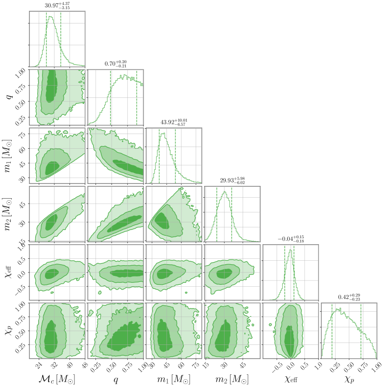
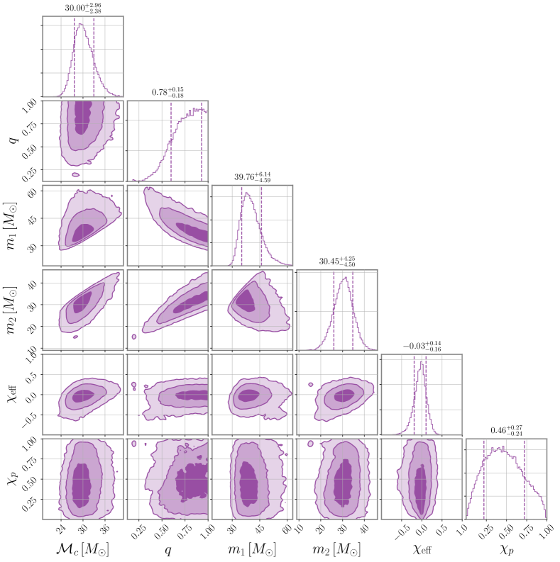
GW170425 and GW170727 are consistent with being generated by heavy BBHs with source frame chirp masses $\mathcal{M}\approx 30M_{\odot}$ and effective aligned spins $\chi_{\rm eff}\sim 0$, in broad agreement with the population of binaries observed in GWTC-1 Abbott et al. (2019c). We report the measured parameters of these three events in Appendix C and Figures 8, 9, 10, and 11.

Of the remaining candidates reported in Venumadhav et al. (2019b), we find that only GW170403 is of marginal interest, with an astrophysical probability $P(\mathcal{S}|\mathbf{d})=0.27$. The other two candidates, GW170202 and GW170304, have a $P(\mathcal{S}|\mathbf{d})$ comparable to GW170818.

The final two event candidates found in the IAS search, GWC170402 and GW170817A, were first reported in Zackay et al. (2019a), a search targeting compact binary mergers that produce a clear signal in one of the detectors and a marginal signal in the other detectors. As per the discussion for GW170818, we do not expect the astrophysical signal probability returned by our framework to be large, finding $P(\mathcal{S}|\mathbf{d})\sim 0$ and $0.02$ respectively. Unlike GW170818, the Bayesian coherence ratio also significantly disfavours these events, with $\log_{10}\mathcal{B}_{\rm cr}$ being more than an order of magnitude smaller.

III.3 Binaries Reported by the PyCBC Search

As per the event candidates reported by the IAS search, we find that only the three events reported in the PyCBC catalogue Nitz et al. (2019), GW170121, GW170425 and GW170727 are of interest. All other event candidates have negligible astrophysical probability. The PyCBC reported $p_{\rm astro}$ is $\sim 1$ for GW170121, $\sim 0.21$ for GW170425, and $\sim 0.99$ for GW170727.

The other significant event reported in Nitz et al. (2019) is GW170304, which was assigned $p_{\rm astro}=0.7$ but for which we find that the astrophysical signal hypothesis is disfavoured with $P(\mathcal{S}|\mathbf{d})=0.03$.

Figure 3: The minimum $P(\mathcal{S})$, which scales linearly with the total astrophysical merger rate integrated over the entire population, required to obtain a probability that the signal is of astrophysical origin $P(\mathcal{S}|\mathbf{d})>0.5$ as a function of the glitch probability $P(\mathcal{G}_{k}|\mathcal{N})$. Here we scale the fiducial values $P(\mathcal{G}_{k}|\mathcal{N})$ by a factor $N\in\left[10^{-2},10^{2}\right]$, keeping the ratio of the glitch probabilities between the detectors fixed, where the ratio is set by the values reported in Table 2. The left panel shows all confident events identified in GWTC-1 and GW190412. The middle panel shows all other triggers listed in Table. 1. The right panel shows a subset of interesting events, including the three most interesting triggers identified: GW170121, GW170425 and GW170727. The grey shaded regions denote the range of values $P(\mathcal{S})$ can take by varying the inferred local merger rate $\mathcal{R}_{0}$ over its 90% credible interval  Abbott et al. (2019c). The vertical dashed lines denote the fiducial values of $P(\mathcal{G}_{k}|\mathcal{N})$.

III.4 Sensitivity of Results to Priors

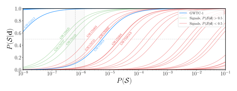
In Fig. 1 we show how sensitive $P(\mathcal{S}|\mathbf{d})$ is to the choice of the prior probability on the signal, $P(\mathcal{S})$. Even if we reduce the value of $P(\mathcal{S})$ by two orders of magnitude, we find that $P(\mathcal{S}|\mathbf{d})\approx 1$ for all GWTC-1 BBHs, with the exception of GW151012, which would be recorded with $P(\mathcal{S}|\mathbf{d})\approx 0.6$, and GW170818, whose value would be $\approx 0$ as per the discussion above.

The astrophysical signal probability of GW170121 and GW170425 is always above 0.5, even when taking the lowest value of $P(\mathcal{S})$ compatible with the 90% probability interval of the local BBH merger rate ${\cal R}_{0}$. For GW170727, the result drops just below our arbitrary threshold of $0.5$ to $P(\mathcal{S}|\mathbf{d})\approx 0.4$. A signal prior $P(\mathcal{S})$ that were at least an order of magnitude higher would yield $P(\mathcal{S}|\mathbf{d})>0.5$ for GW170403, GW170721 and GW170202.

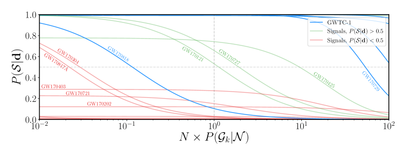
In Fig. 2 we explore how sensitive the results are to the prior probability of the glitch hypothesis at a fixed signal probability corresponding to the value in Eq. (2). Again, all the GWTC-1 BBHs, with the usual exception of GW170818, are fairly insensitive to variations in $P(\mathcal{G}_{k}|\mathcal{N})$ by at least a factor of 100.

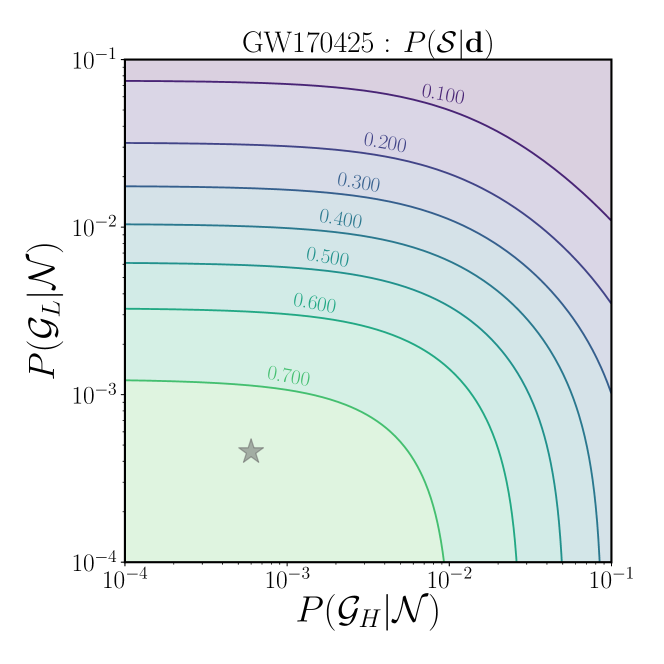
For GW170425, one would need to increase the glitch probability by a factor $\approx 10$ to reduce $P(\mathcal{S}|\mathbf{d})$ below 0.5.

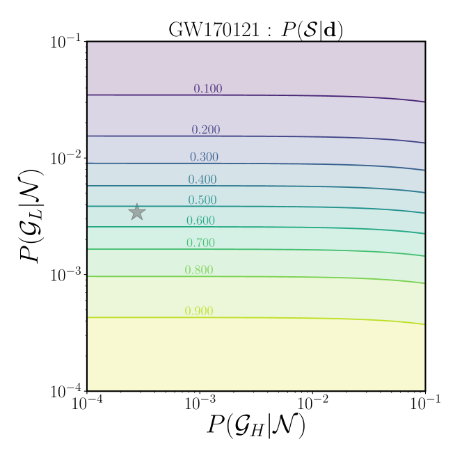
In particular GW170121, but also GW170727, are much more sensitive to variations in $P(\mathcal{G}_{k}|\mathcal{N})$. Increasing the glitch prior $P(\mathcal{G}_{k}|\mathcal{N})$ by a factor of $\approx 2-3$ would reduce $P(\mathcal{S}|\mathbf{d})$ to below 0.5.

Interestingly, $P(\mathcal{S}|\mathbf{d})$ for GW170403, GW170721 and GW170202 is insensitive to the glitch probability in the region considered here: the signals are weak, and as discussed above $P(\mathcal{S}|\mathbf{d})$ is driven by the prior signal probability.

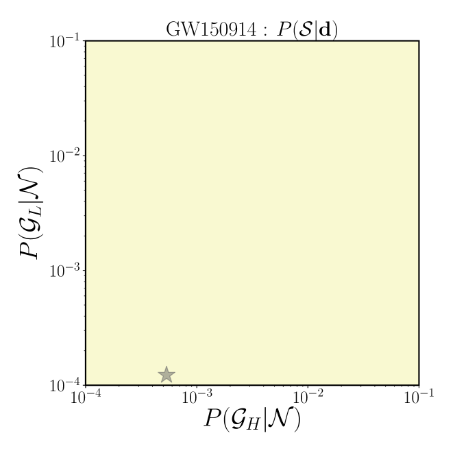
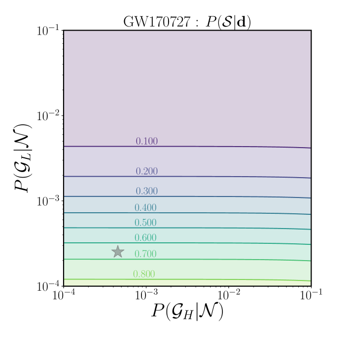
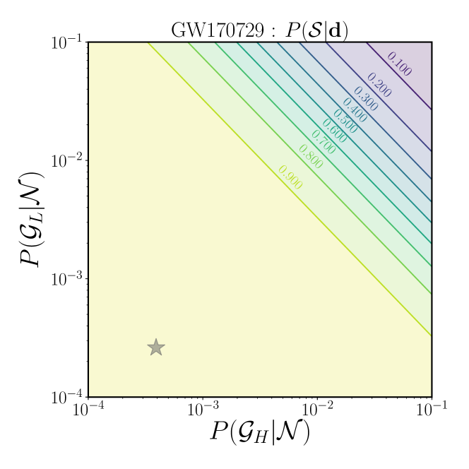
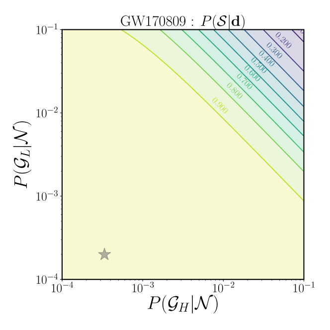
In Appendix B and Fig. 7, we provide additional diagnostics for a subset of events, including GW170425, GW170121 and GW170227, to show how $P(\mathcal{S}|\mathbf{d})$ varies in the $P(\mathcal{G}_{L}|\mathcal{N})-P(\mathcal{G}_{H}|\mathcal{N})$ plane.

A complementary way of exploring how the astrophysical signal odds and associated signal posterior probability depend on the signal and glitch prior probabilities is displayed in Fig. 3. We show the minimum $P(\mathcal{S})$ required to obtain an astrophysical probability of $P(\mathcal{S}|\mathbf{d})>0.5$ as a function of the glitch probability $P(\mathcal{G}_{k}|\mathcal{N})$, where the ratio of $P(\mathcal{G}_{k}|\mathcal{N})$ between the detectors is kept constant, and set by the values reported in Table 2. The left panel of Fig. 3 shows all confident GWTC-1 events plus GW190412. The middle panel shows all remaining triggers, with the three most compelling events GW170121, GW170425 and GW170727 highlighted in green. The right panel of Fig. 3 focuses on a subset of interesting events. We show GW150914 and GW190412 as clear, unambiguous detections where even increasing the glitch rate by a factor $\sim\mathcal{O}(10^{2})$ is insufficient to disfavour the astrophysical hypothesis. GW151012 was initially identified with a high false alarm rate (FAR) Abbott et al. (2016e) but improvements to the analysis pipelines used for the GWTC-1 re-analysis of this event substantially reduced the FAR, leading to a $p_{\rm astro}=0.96$ Abbott et al. (2019a). In our Bayesian framework, GW151012 is unambiguously identified as an astrophysical signal with $P(\mathcal{S}|\mathbf{d})\sim 0.99$, in agreement with Isi et al. (2018); Ashton and Thrane (2020) and showcasing the utility of our unified framework for calculating the astrophysical signal probability. Finally, we highlight the three most compelling events from our analysis presented: GW170121, GW170425 and GW170727.

The horizontal shaded area in Fig. 3 denotes the allowed range of the prior probability on the signal as inferred from Eq. (13) obtained by varying the local astrophysical merger rate $\mathcal{R}_{0}$ over its $90\%$ confidence interval. For all events with significant support for the astrophysical signal hypothesis, the minimum $P(\mathcal{S})$ required to meet the threshold of $0.5$ is far below the astrophysical rate estimated in App. A for typical glitch rates estimated from the distribution of Omicron triggers, with an upper limit on the glitch prior of $P(\mathcal{G}_{k}|\mathcal{N})\sim\rm{few}\times 10^{-3}$. As an interesting case study, for GW170729 we would need to increase the glitch rate by a factor of $\sim 10^{2}$ before $P(\mathcal{S}|\mathbf{d})$ starts to drop below $0.5$, emphasising the robustness of this result.

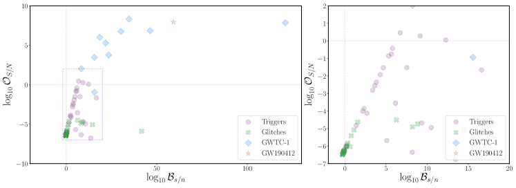
It would be reasonable to wonder if our approach is robust against noise transients of instrumental origin that pollute the data. In Fig. 4, we show the Bayes factor for the signal to noise hypothesis $\mathcal{B}_{s/n}$ against the astrophysical signal odds $\mathcal{O}_{S/N}$ for all triggers listed in Tab. 1. In addition, we plot the same quantities evaluated for a population of known glitches identified by the PyCBC search. Figure 4 serves to demonstrate the efficacy with which the inferred $P(\mathcal{S}|\mathbf{d})$ for glitches is suppressed and as a caution that the standard Bayes factor for signal vs noise $\mathcal{B}_{s/n}$ is a poor discriminator between astrophysical signals and instrumental noise transients.

Figure 4: Bayes factor for the signal to noise hypothesis $\mathcal{B}_{s/n}$ against the astrophyiscal signal odds $\mathcal{O}_{S/N}$ for all events in GWTC-1 (blue), GW190412 (orange), the candidate events listed in Tab. 1 (red) and a set of known glitches (green). Despite relatively high signal-to-noise Bayes factors, the astrophysical signal odds for the population of known glitches is efficiently suppressed within this framework. In the left panel we show all triggers and in the right panel we focus on the boxed region region demarcated by the purple dashed lines.

Figure 5: The 1D and 2D posterior distributions for the hyperparameters describing the BBH population model for the masses and rates. Here the blue posteriors denote the results of the analysis considering all GWTC-1 events in the population analysis. The red posteriors show the results when including the three events with $P(\mathcal{S}|\mathbf{d})>0.5$, GW170121, GW170425 and GW170727 in addition to all GWTC-1 events. The green posteriors refer to the inferred population based on all GWTC-1 events plus all triggers reported in Zackay et al. (2019a, b, c); Venumadhav et al. (2019a) irrespective of $P(\mathcal{S}|\mathbf{d})$. We also report the 1D median values and 90% probability interval inferred using all GWTC-1 binaries plus the three events with $P(\mathcal{S}|\mathbf{d})>0.5$.

IV Implications for Population Inference

In our Bayesian analysis, we have identified three additional event candidates with a $P(\mathcal{S}|\mathbf{d})>0.5$ (see Table 1), which would be sufficient for inclusion in typical population studies Abbott et al. (2019a, c). In this section, we assess the impact of including GW170121, GW170425 and GW170727 on the inferred BBH population properties Abbott et al. (2019c).

Following the methodology described in Abbott et al. (2019c), we perform hierarchical Bayesian inference, incorporating measurement uncertainty and selection effects into the analysis Abbott et al. (2016f); Wysocki et al. (2019); Mandel et al. (2019); Fishbach et al. (2018). The rate of events is modeled as a Poisson process whose mean is dependent on the parameter distribution of the population of binary black holes

$$\mathcal{L}(\{d_{n}\}|\Lambda) \propto e^{-\mu(\Lambda)}\displaystyle\prod^{N_{\rm obs}}_{n=1}\mathcal{L}(d_{n}|\theta,z)\frac{dN}{d\theta dz}(\Lambda)\,d\theta\,dz,$$ (16)

where $\theta$ are the intrinsic parameters of the binary, $z$ the redshift, $N$ the total number of mergers that occur within the detection horizon, and $\mu(\Lambda)$ the rate constant describing the mean number of events as a function of the population hyperparameters $\Lambda$. Here $N_{\rm obs}$ is the number of detections and the individual-event likelihood for the $n^{\rm th}$ detection is $\mathcal{L}(d_{n}|\theta,z)$. The expected number of events is dependent on the selection effects for the detectors. This can be characterised by the sensitive spacetime volume $VT(\theta)$ for a detector network in terms of the detection probability for a binary with parameters $\theta$ and the total observation time, as discussed in App. A.

Figure 6: The 1D and 2D posterior distributions for the hyperparameters describing the spin population model. As per Fig. 5, the blue posteriors denotes all GWTC-1 events. The red posteriors show all GWTC-1 events plus the three events with $P(\mathcal{S}|\mathbf{d})>0.5$, GW170121, GW170425 and GW170727. The green posteriors show all GWTC-1 events plus all triggers reported in Zackay et al. (2019a, b, c); Venumadhav et al. (2019a). We report the 1D median values and 90% probability interval inferred using all GWTC-1 binaries plus the three events with $P(\mathcal{S}|\mathbf{d})>0.5$.

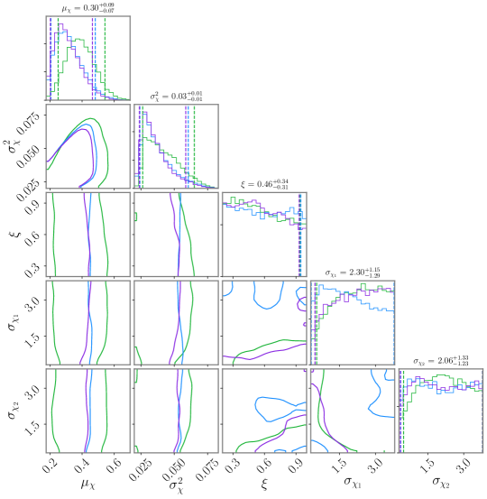
For the population inference, we use Model C of Abbott et al. (2019c) as a representative model. This model is based on a power law mass distribution with an additional Gaussian component at high masses Talbot and Thrane (2018). The low-mass cutoff $m_{\rm min}$ is tapered by a smoothing scale $\delta m$ to account for environmental effects, such as metallicity, that can blur the edge of the lower mass gap Talbot and Thrane (2018); Abbott et al. (2019c) and the maximum allowed BH mass is given by $m_{\rm max}$. At low masses, we recover a standard mass power-law governed by a power-law index $\alpha$ on the primary BH and a mass ratio power-law index $\beta_{q}$. The Gaussian component models the possible build up of high-mass BBHs from pulsational pair-instability supernovae Barkat et al. (1967); Woosley and Weaver (1986); Heger and Woosley (2002); Chatzopoulos and Wheeler (2012); Woosley (2017) and is parameterized by the mean $\mu_{m}$ and standard deviation $\sigma_{m}$ and well as the fraction of primary BHs in the Gaussian component $\lambda_{m}$. The distribution of spin magnitudes $\chi_{i}$ is taken to be drawn from a beta distribution Wysocki et al. (2019) and can be parameterized by either the moments of the distribution $\alpha_{\chi}$ and $\beta_{\chi}$ or, equivalently, by the mean $\mu_{\chi}$ and variance $\sigma^{2}_{\chi}$. The distribution of spin orientations is modelled as a mixture of two distributions corresponding to an isotropic and a preferentially aligned component Talbot and Thrane (2017). The fraction of binaries preferentially aligned with the orbital angular momentum is denoted $\xi$ and the degree of spin misalignment is denoted by $\sigma_{\chi_{i}}$. The redshift evolution of the model follows the prescription in Fishbach et al. (2018), where, for simplicity, we assume a merger rate density that is uniform in comoving volume and source-frame time.

The likelihood $\mathcal{L}(d_{n}|\theta,z)$ is recycled from the posterior samples calculated using LALInference Veitch et al. (2015). We assume uniform priors on the population parameters, as detailed in Table 2 of Abbott et al. (2019c). For the event rate, we take a log-uniform distribution bounded between $\left[10^{-1},10^{3}\right]$. The hierarchical population inference is carried out using the gwpopulation package Talbot et al. (2019) and Bilby Ashton et al. (2019a).

As a proxy for incorporating full information regarding the astrophysical signal probability, we use the posterior probability of the signal hypothesis $P(\mathcal{S}|\mathbf{d})$ as a criterion for including events in our population inference. Following Abbott et al. (2019a, c), the threshold is taken to be $P(\mathcal{S}|\mathbf{d})>0.5$. Based on the analysis discussed in Sec. III, the events GW170121, GW170425 and GW170727 satisfy this selection criterion for our default priors and we can incorporate them into the hierarchical inference.

Some approaches for incorporating $p_{\rm astro}$ in hierarchical population inference have recently been presented in Gaebel et al. (2019); Galaudage et al. (2019). The framework presented in Galaudage et al. (2019) also allows for $p_{\rm astro}$ to be revised by taking into account information regarding the distribution of black hole masses and spins from the observed population of binaries. Applying this method to all GWTC-1 candidates, as well as the 8 binaries reported in Zackay et al. (2019c); Venumadhav et al. (2019b, a), Galaudage et al. (2019) determine that all binaries have a $p_{\rm astro}\sim 1$. This places the results in some tension with the results presented here and in Ashton and Thrane (2020). Whilst a detailed re-analysis of the impact of $p_{\rm astro}$ on population inference is beyond the scope of this paper, it seems plausible that discarding information regarding the coherence of the signal is in part culpable for the discrepancies observed and could lead to a non-trivial bias in the inferred astrophysical merger rate.

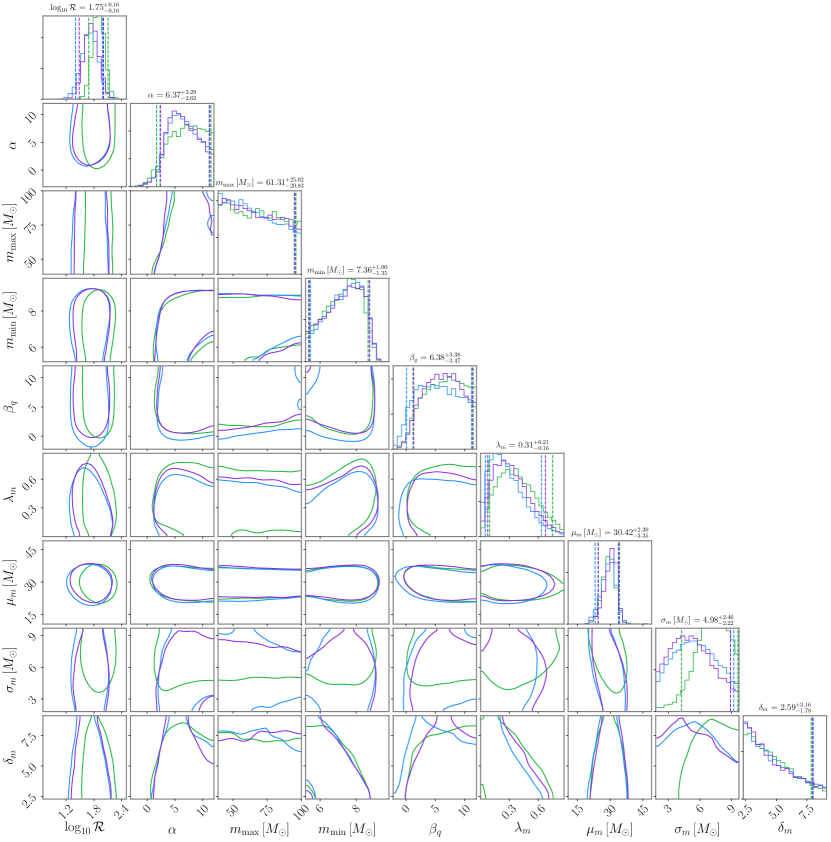
In Figures 5 and 6 we compare the posterior distributions for the mass and spin population hyperparameters, respectively, by including in the population study: (i) GWTC-1 binaries alone (blue curves), (ii) GWTC-1 binaries and the three new event candidates with significant astrophysical probability as determined by our analysis (purple curves), and (iii) GWTC-1 binaries and all binaries reported in the IAS search, excluding GW170402, irrespective of $P(\mathcal{S}|\mathbf{d})$ as in Galaudage et al. (2019). The population hyperparameters inferred from GWTC-1 plus the three new events are in broad agreement with the results inferred using the GWTC-1 binaries alone. We see a slight shift to higher values of the astrophysical merger rate $\mathcal{R}_{0}$ and some of the other hyperparameters, notably the degree of spin misalignment for the primary BH $\sigma_{\chi_{1}}$.

Incorporating the 8 IAS event candidates, we find that the population hyper-parameters are increasingly discrepant with respect the results from using GWTC-1 alone. In particular, we observe that the astrophysical merger rate $\mathcal{R}_{0}$, the width of the Gaussian mass peak $\sigma_{m}$ and the mean of the spin magnitude distribution $\mu_{\chi}$ shift quite significantly. We observe the same shift in $\sigma_{\chi_{1}}$ as when including the 3 events with significant astrophysical probability returned by our analysis.

Incorporating information regarding the coherence of the signal will likely be an important consideration when performing population inference on an ever growing catalog of observed compact binaries. This highlights the necessity of a robust, unified framework for calculating the astrophysical signal odds agnostic to any specific search pipeline of strategy, such as the framework presented here.

V Discussion

We have revisited the problem of determining whether an observed GW transient is due to an astrophysical source. We employ a Bayesian framework to derive the posterior odds ratio, $\mathcal{O}_{S/N}$, allowing us to determine the probability that the signal is of astrophysical origin, $P(\mathcal{S}|\mathbf{d})$, independent of any search pipeline. The astrophysical posterior odds is determined through a coherent analysis of the data, depending only on the underlying model hypotheses and the choice of prior probabilities. In order to set the astrophysical signal prior $P(\mathcal{S})$, we leveraged prior knowledge on the population of astrophysical BBHs. The glitch probability for a given detector $P(\mathcal{G}_{k}|\mathbf{d})$ was determined using the density of Omicron triggers in a 24h stretch of data around each event, allowing us to account for asymmetric noise profiles between the detectors and for changes in the behaviour of the detectors over time. This work builds on recent studies in the literature Veitch and Vecchio (2010); Isi et al. (2018); Ashton et al. (2019a, b).

We analyse all confident BBH events reported in GWTC-1 Abbott et al. (2019a) as well as event candidates recently reported by independent search pipelines Venumadhav et al. (2019b); Zackay et al. (2019c, a); Nitz et al. (2019, 2020). Using the astrophysical posterior odds $\mathcal{O}_{S/N}$, we find that all GWTC-1 binaries, except for the single detector event GW170818, have overwhelming odds in favour of the astrophysical signal hypothesis. Of all other event candidates analyzed, only GW170121, GW170425 and GW170727 have odds in favour of the astrophysical signal hypothesis, $P(\mathcal{S}|\mathbf{d})>0.5$, meeting the threshold for inclusion in typical population studies Abbott et al. (2019c). We characterized the robustness of these results to changes in the signal $P(\mathcal{S})$ and glitch $P(\mathcal{G}_{k}|\mathcal{N})$ priors. Due to the significant computational burden of our analysis, in this paper we have considered only BBH candidates; our method however is fully general and can be applied to all classes of binary systems.

The methodology presented in this paper can be further improved in a number of ways. Due to the limited coincident data available, and the non-trivial computational processing load we restricted our analysis to a 2-detector network. As the duty cycle of the instruments improves, the analysis should incorporate data from all available detectors in a given network at any given time. The fourth observing run (O4) is scheduled to last for one year, with the LIGO detectors nearing design sensitivity and Phase 1 of the Advanced VIRGO+ upgrade nearing completion Abbott et al. (2018b). In addition, KAGRA Aso et al. (2013); Akutsu et al. (2019) will be operational with a nominal BNS range of $25-130\rm{Mpc}$ Abbott et al. (2018b), providing the potential opportunity for analysing coherent data from 4 detectors. The discriminating power of our approach between astrophysical signals and instrumental transient will correspondingly increase as data from more instruments are included.

With detector sensitivities ever increasing, the approximation that signals and glitches do not overlap can break down, as was the case for GW170817 Abbott et al. (2017). Whilst glitch subtraction can be an effective tool to mitigate such scenarios Cornish and Littenberg (2015), the model will need to be generalised to include this possibility, and in the future even contemplate the possibility of overlapping astrophysical signals.

For computational efficiency, we used the precessing waveform model IMRPhenomPv2 Hannam et al. (2014); Schmidt et al. (2015); Husa et al. (2016); Khan et al. (2016). In future analyses, we plan to utilise improved and more accurate waveform models Pratten et al. (2020a) that incorporate both higher modes Nagar et al. (2020a, b); García-Quirós et al. (2020a) and precession Pratten et al. (2020b); Ossokine et al. (2020). As a first step, we have re-analysed GW170121, GW170425 and GW170727 with the precessing higher-mode waveform model PhenomXPHM Pratten et al. (2020b), while keeping all the other parameters of our analysis unchanged. We find that $P(\mathcal{S}|\mathbf{d})$ increases from $0.53$ to $0.56$ for GW170121, from $0.74$ to $0.84$ for GW170425, and from $0.66$ to $0.67$ for GW170727.

To process large catalogues of candidate events or inferring $P(\mathcal{S}|\mathbf{d})$ in low-latency – the latter can be done with rather minor changes to the present implemented software infrastructure and relatively small additional computational cost – it will be important to adopt methods that further reduce waveform generation costs Vinciguerra et al. (2017); García-Quirós et al. (2020b) and mitigate the computational cost of the Bayesian inference Canizares et al. (2015); Smith et al. (2016).

Due to the lack of a robust glitch model, we made the simplifying approximation that $\mathcal{G}_{k}\approx\mathcal{S}_{k}$. Whilst this is the most conservative choice that could be made Veitch and Vecchio (2010), our understanding of the instruments’ behaviour is continuously improving, as is our ability to classify and describe glitches. In the future, a reliable glitch model could be available and allow us to more adequately distinguish between astrophysical signals and glitches, thereby increasing the significance of the inferred $P(\mathcal{S}|\mathbf{d})$.

The astrophysical signal prior $P(\mathcal{S})$ used in this analysis was determined by calculating the expected number of observed BBHs within the relevant time span from a population of binaries taking into account selection effects, see Eq. (20). A more detailed characterization of the detector sensitivity $\langle VT\rangle_{\Lambda}$, e.g. through Monte-Carlo integration Tiwari (2018); Abbott et al. (2019c) or novel applications of machine-learning Gerosa et al. (2020), could allow for a more accurate determination of $P(\mathcal{S})$ as a function of the population hyperparameters $\Lambda$. In addition our analysis can be improved by dividing the whole observing period into shorter segments, and updating $P(\mathcal{S})$ as the analysis progresses. Finally, the default priors used in calculating the Bayes factors are uniform in the component masses, uniform in spin magnitudes and isotropic in spin orientations. The use of such agnostic priors is of particular importance in the absence of any a priori knowledge about the expected shape of the distributions. However, as the number of observations increases, it will be important to consider population informed priors, e.g. by constructing the posterior predictive distributions Fishbach et al. (2020); Galaudage et al. (2019).

Appendix A Calculation of the signal prior probability

Here we provide details of the calculation of the prior signal probability, $P(\mathcal{S})$, given by Eq. (13).

In order to calculate the expected number of detections $\mu(\Lambda)$, we need to incorporate selection effects from a network of detectors. Here, we calculate the sensitive spacetime volume $\langle VT\rangle$ following a semi-analytic prescription Finn and Chernoff (1993); Abbott et al. (2016e, 2019c). For a network of gravitational wave detectors, the sensitive spacetime volume is

$$VT(\theta) =T_{\rm obs}\displaystyle\int^{z_{\rm max}}_{0}f(z|\theta)\frac{dV_{c}}{dz}\frac{1}{1+z}\,dz$$ (17)

where we assume a constant sensitivity over an observing run $T_{\rm obs}$ and $f(z|\theta)$ is the detection probability for a binary with parameters $\theta$ at a redshift $z$ O’Shaughnessy et al. (2010) averaged over extrinsic parameters Finn and Chernoff (1993). For each binary, we calculate the optimal SNR $\rho_{\rm opt}$ using the IMRPhenomXAS phenomenological waveform model Pratten et al. (2020a), corresponding to the SNR that would be observed for a face-on source located directly overhead a detector. For an isotropic distribution of sources, with arbitrary sky locations and inclinations, the distribution of SNRs can be captured by introducing a coefficient $\Theta$ that parameterizes the angular dependence, $0\leq\Theta=\rho/\rho_{\rm opt}$, and where $\Theta$ has a known distribution Finn and Chernoff (1993). Here $\Theta=1$ corresponds to an optimally oriented source and $\Theta=0$ corresponds to a binary that is in a blind spot of the detector. The probability of detecting a source at a redshift $z$ can therefore be written as

$$f(z|\theta) \equiv p_{\rm det}(z|\theta)=P(\rho\geq\rho_{\rm th}),$$ (18)

where $\rho_{\rm th}$ is the threshold for observing a binary. Here we assume that sources will only be detected if they have a single detector SNR above a threshold $\rho_{\rm ifo}>7$.

We incorporate both mass and spin dependence in the calculation of $VT(\theta)$, though spins have a subdominant effect on the $\rho$ calculation for the population of binaries considered here Abbott et al. (2019c). For a given population with hyper-parameters $\Lambda$, the total sensitive spacetime volume is Abbott et al. (2019c)

$$\langle VT\rangle_{\Lambda} =\displaystyle\int_{\theta}p(\theta|\Lambda)\,VT(\theta)\,d\theta.$$ (19)

If the merger rate evolves with redshift, the expected number of detections will be given by

$$\mu(\Lambda) =T_{\mathrm{obs}}\int_{\theta}\int_{0}^{\infty}p(\theta|\Lambda)f(z|\theta)\mathcal{R}(z)\frac{\mathrm{d}V_{c}}{\mathrm{d}z}\frac{1}{1+z}\mathrm{d}z\,\mathrm{d}\theta.$$ (20)

Following Fishbach et al. (2018), we can parameterize the evolving merger rate density $\mathcal{R}(z)$ in the comoving frame by

$$\mathcal{R}(z|\lambda) =\mathcal{R}_{0}(1+z)^{\lambda},$$ (21)

where $\mathcal{R}_{0}$ is the local merger rate density at $z=0$. Here, $\lambda=0$ corresponds to a uniform in comoving volume merger rate and $\lambda\sim 3$ is a merger rate that approximately follows the star formation rate Madau and Dickinson (2014), at redshifts below $z\approx 2$, which corresponds to the peak of the star formation rate. For the population of binaries here, we take $\lambda=2$, consistent with Abbott et al. (2019c, 2020a). In the simpler scenario in which the merger rate is constant with redshift, the expected number of observations reduces to

$$\mu(\Lambda) =\mathcal{R}_{0}\,\langle VT\rangle_{\Lambda}.$$ (22)

The expectation value of $VT(\theta)$ can be calculated using standard Monte Carlo methods

$$\langle VT\rangle_{\Lambda} =\displaystyle\int p(\theta|\Lambda)\,VT(\theta)\,d\theta\approx\frac{1}{N}\displaystyle\sum^{N}_{k}VT(\theta_{k}).$$ (23)

We use PSDs that are representative of the detector performance in O2 Abbott et al. (2019a); LIGO Scientific Collaboration, Virgo Collaboration (2019) and assume a total coincident observing time of $T_{\rm obs}=0.46\rm{y}$ Abbott et al. (2019a). For the population of binaries, we use a parameterized mass model

$$p(m_{1},m_{2}|m_{\rm min},m_{\rm max},\alpha,\beta_{q})\propto C(m_{1})m_{1}^{-\alpha}\,q^{\beta_{q}},$$ (24)

where the minimum and maximum black hole masses are taken to be $m_{\rm min}=5M_{\odot}$ and $m_{\rm max}=50M_{\odot}$, as motivated by the apparent lower limit for X-ray binary observations Farr et al. (2011) and the maximum mass above which a pair-instability supernova is thought to completely disrupt the star Barkat et al. (1967). The slope of the mass power law is taken to be $\alpha=1.8$ and the exponent for the mass ratio to be $\beta_{q}=2.0$, in broad agreement with Abbott et al. (2019c, 2020a). The distribution of spin magnitudes $\chi_{i}$ are taken to follow a beta distribution Wysocki et al. (2019)

$$p\left(\chi_{i}|\alpha_{\chi},\beta_{\chi}\right)=\frac{\chi_{i}^{\alpha_{\chi}-1}\left(1-\chi_{i}\right)^{\beta_{\chi}-1}}{\mathrm{B}\left(\alpha_{\chi},\beta_{\chi}\right)},$$ (25)

with $\alpha_{\chi}=1.5$ and $\beta_{\chi}=3.5$. The spin orientations are taken to follow a mixture model consisting of an isotropic component and a preferentially aligned component Talbot and Thrane (2017)

$$p\left(\cos t_{1},\cos t_{2}|\sigma_{1},\sigma_{2},\zeta\right) =\frac{(1-\zeta)}{4}$$

$$+\frac{2\zeta}{\pi}\prod_{i\in\{1,2\}} \frac{\exp\left(-\left(1-\cos t_{i}\right)^{2}/\left(2\sigma_{i}^{2}\right)\right)}{\sigma_{i}\operatorname{erf}\left(\sqrt{2}/\sigma_{i}\right)},$$ (26)

where we take $\zeta=0.5$ and $\sigma_{i}=1$. In practice, we only use the spins projected along the orbital angular momentum $\vec{L}$ when evaluating the aligned-spin waveform model to calculate the SNR.

Using the population of binaries detailed above, the sensitive spacetime volume is estimated to be

$$\langle VT\rangle_{\Lambda} \approx 0.877\;\rm{Gpc}^{3}\;\rm{y}.$$ (27)

Using a fiducial local astrophysical merger rate of $\mathcal{R}_{0}=53.2\,\rm{Gpc}^{-3}\,\rm{y}^{-1}$ Abbott et al. (2019c), the probability of a signal within a coalescence interval of $0.2s$ yields Eq. (13).

Appendix B Impact of glitch prior probability on the posterior signal probability of a signal

In Table 2 we report the glitch probability for each of the two instruments that we have used in the analysis, see Tab. 1, and we also report the SNRs (signle detector and across the network) for each of the candidate events.

In Fig. 7 we explore the dependence of $P(\mathcal{S}|\mathbf{d})$ on the glitch prior for each of the detectors for selected events. The fiducial values of $P(\mathcal{G}_{k}|\mathbf{d})$ estimated from the Omicron triggers are denoted with a grey star.

Appendix C Posteriors for GW170121, GW170425 and GW170727

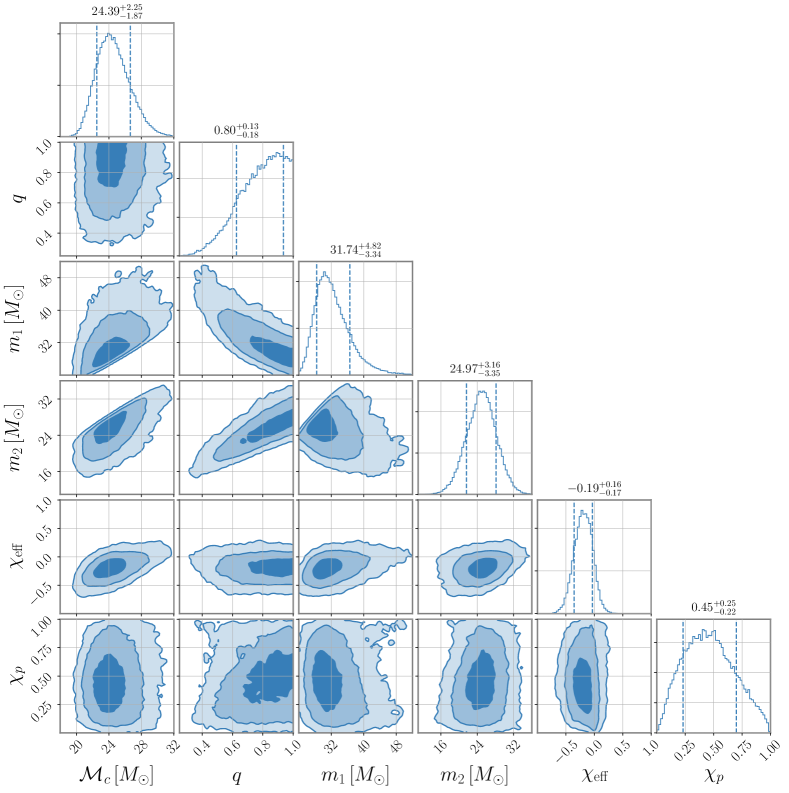
In Fig. 8, 9 and 10 we show the posterior distributions for a subset of key intrinsic parameters for the three candidate events with $P(\mathcal{S}|\mathbf{d})>0.5$: GW170121, GW170425 and GW170727. The posterior distributions show that the instrinsic parameters of the BBHs that generated these systems are broadly compatible with those that characterise the population of BBHs observed in O1 and O2 as reported in GWTC-1 Abbott et al. (2019a, c), though we note that GW170121 has a negative effective aligned spin paameter $\chi_{\rm eff}\simeq-0.22^{+0.17}_{-0.17}$ Venumadhav et al. (2019b); Huang et al. (2020).

In Fig. 11, we perform a sanity check on the posterior distributions for the three events with $P(\mathcal{S}|\mathbf{d})>0.5$, GW170729 – which was reported in GWTC-1 with different values of $p_{\mathrm{astro}}$ by different pipelines – and GW150914, an unambiguous BBH. For a coherent astrophysical signal, the posterior distributions for parameters that can be well constrained from the data should be broadly consistent between the values inferred from each detector individually as well as the coherent network analysis. GW150914 and GW170728 both show significant information gain from Hanford and Livingston respectively. The posteriors for the new events of interest show that information is gained from each detector individually.

Table 2: The first three columns show the network signal-to-noise ratio and single detector signal-to-noise ratio (the indices “L” and “H” stand for LIGO-Livigston and LIGO-Hanford, respectively) for all the events considered in this analysis, see Tab. 1. The next three columns show the Bayes factors for the signal vs noise hypothesis for the detector network, Eq. (5), and the single detectors, Eq. (4), respectively. The last two columns report the glitch probabilities as estimated from Omicron triggers in a 24h stretch of data near each trigger. The glitch rates are determined by down-selecting Omicron triggers based on a single detector signal-to-noise ratio threshold of $\rho>7$ and by restricting the frequencies to $20<f_{\textsc{Om}}<1024$Hz, see Eq. (15) and discussion in Sec. II.2.

Event	$\rho^{\rm Net.}_{\rm MF}$	$\rho^{H}_{\rm MF}$	$\rho^{L}_{\rm MF}$	$\log_{10}\mathcal{B}_{s/n}$	$\log_{10}\mathcal{B}^{(H)}_{s/n}$	$\log_{10}\mathcal{B}^{(L)}_{s/n}$	$P(\mathcal{G}_{H}|\mathcal{N})$	$P(\mathcal{G}_{L}|\mathcal{N})$
GW150914	25.01	20.30	14.71	121.1	77.77	36.45	$5.35\times 10^{-4}$	$1.23\times 10^{-4}$
GW151012	9.63	7.23	6.38	8.25	1.97	0.77	$8.73\times 10^{-4}$	$3.61\times 10^{-4}$
GW151226	12.71	10.30	7.35	18.45	9.26	0.23	$9.42\times 10^{-4}$	$1.74\times 10^{-4}$
GW170104	14.01	9.75	10.27	30.19	10.96	12.85	$6.16\times 10^{-4}$	$4.42\times 10^{-4}$
GW170608	15.62	12.68	9.82	34.7	19.45	7.46	$5.00\times 10^{-4}$	$3.82\times 10^{-4}$
GW170729	10.62	9.15	7.34	15.52	7.4	5.46	$3.91\times 10^{-4}$	$2.62\times 10^{-4}$
GW170809	12.82	7.77	11.01	23.44	3.47	16.88	$3.36\times 10^{-4}$	$1.99\times 10^{-4}$
GW170814	16.66	9.27	14.08	46.32	8.96	31.56	$2.50\times 10^{-4}$	$2.22\times 10^{-4}$
GW170818	11.34	3.70	10.58	15.58	0.05	13.97	$2.96\times 10^{-4}$	$2.27\times 10^{-4}$
GW170823	12.04	7.19	9.93	21.72	3.97	13.54	$2.06\times 10^{-4}$	$1.67\times 10^{-4}$
GW151011	7.46	4.05	6.18	4.3	0.28	2.45	$8.73\times 10^{-4}$	$3.31\times 10^{-4}$
GW151124	8.67	4.99	8.80	5.1	-0.28	7.76	$4.40\times 10^{-4}$	$6.90\times 10^{-4}$
GW151205	6.81	5.43	4.77	4.67	1.57	1.04	$6.81\times 10^{-4}$	$7.55\times 10^{-4}$
GW151216	8.16	5.41	6.10	3.84	0.36	0.51	$9.24\times 10^{-4}$	$1.81\times 10^{-4}$
GW151216A	8.48	6.88	4.52	0.18	-0.08	-0.09	$9.24\times 10^{-4}$	$1.71\times 10^{-4}$
GW151217	7.99	5.59	3.55	0.15	-0.11	0.04	$9.24\times 10^{-4}$	$1.71\times 10^{-4}$
GW151222	10.22	10.50	3.50	9.34	10.86	0.13	$9.24\times 10^{-4}$	$1.71\times 10^{-4}$
GW170104A	7.36	5.76	5.13	1.37	0.05	0.34	$6.16\times 10^{-4}$	$4.42\times 10^{-4}$
GW170106	9.62	10.05	2.90	8.19	11.15	-0.09	$1.58\times 10^{-3}$	$1.05\times 10^{-3}$
GW170121	10.55	5.43	9.04	12.26	0.4	8.49	$2.78\times 10^{-4}$	$3.42\times 10^{-3}$
GW170123	6.20	4.29	5.61	2.34	0.05	0.58	$1.85\times 10^{-4}$	$1.08\times 10^{-3}$
GW170201	8.25	6.44	6.12	3.64	0.36	0.45	$2.64\times 10^{-4}$	$3.19\times 10^{-4}$
GW170202	8.50	5.26	7.29	5.33	0.31	1.48	$3.82\times 10^{-4}$	$3.10\times 10^{-4}$
GW170220	6.59	4.68	4.81	2.18	0.18	0.94	$2.57\times 10^{-4}$	$2.71\times 10^{-4}$
GW170304	8.50	5.75	7.50	7.53	0.46	5.83	$2.20\times 10^{-4}$	$1.04\times 10^{-3}$
GW170402	9.00	3.43	9.29	6.16	0.01	6.67	$2.92\times 10^{-4}$	$7.04\times 10^{-4}$
GW170403	8.20	6.27	6.47	5.8	1.56	1.79	$4.00\times 10^{-4}$	$9.21\times 10^{-4}$
GW170425	7.99	5.75	5.98	6.74	1.69	2.61	$5.99\times 10^{-4}$	$4.56\times 10^{-4}$
GW170620	8.36	6.05	6.11	3.38	0.11	0.33	$8.77\times 10^{-4}$	$3.06\times 10^{-4}$
GW170629	7.56	6.40	3.41	-0.06	-0.12	-0.3	$7.62\times 10^{-4}$	$3.91\times 10^{-4}$
GW170721	8.55	7.13	5.88	5.66	3.08	0.23	$5.51\times 10^{-4}$	$2.87\times 10^{-4}$
GW170724	10.76	11.84	6.27	13.46	17.14	-0.2	$7.87\times 10^{-4}$	$2.69\times 10^{-4}$
GW170727	9.90	4.97	7.66	9.15	0.16	6.27	$4.54\times 10^{-4}$	$2.52\times 10^{-4}$
GW170729A	11.55	11.17	4.35	10.5	12.73	0.7	$3.31\times 10^{-4}$	$2.89\times 10^{-4}$
GW170801	8.14	3.14	8.05	2.69	0.05	4.17	$2.45\times 10^{-4}$	$2.22\times 10^{-4}$
GW170817A	10.65	3.82	10.42	16.62	0.11	15.88	$2.55\times 10^{-4}$	$1.62\times 10^{-4}$
GW190412	18.47	9.77	15.80	59.27	10.59	42.54	$1.00\times 10^{-4}$	$1.00\times 10^{-4}$

Figure 7: Posterior probability that the signal is of astrophysical origin $P(\mathcal{S}|\mathbf{d})$ for select events as a function of the detector glitch probabilities $P(\mathcal{G}_{H}|\mathcal{N})$ and $P(\mathcal{G}_{L}|\mathcal{N})$ for the LIGO-Hanford and LIGO-Livingston instruments, respectively. The grey star denotes the glitch probability estimated from Omicron triggers, see Table 2. GW150914 is unambiguous, having an astrophysical probability $\approx 1$ irrespective of the glitch probability. Similarly, we find that GW170729 has $P(\mathcal{S}|\mathbf{d})\approx 1$ for the glitch probabilities estimated from a $24$h window around the event. For the candidate events GW170121, GW170425 and GW170727, the probability that the signal is of astrophysical origin is more sensitive to prior probability on the glitch and signal hypotheses respectively.

Figure 8: Posterior distributions for GW170121. We show source frame parameters: chirp mass $\mathcal{M}_{c}\equiv(m_{1}\,m_{2})^{3/5}/(m_{1}+m_{2})^{1/5}$, mass ratio $q\equiv m_{2}/m_{1}\leq 1$, component masses $m_{1}$ and $m_{2}$, effective aligned spin $\chi_{\rm eff}$ and effective precessing spin $\chi_{p}$ Schmidt et al. (2015), see e.g. Eq. (6) and (9), respectively, in Abbott et al. (2016g). Note that whilst GW170121 has negative effective spin $\chi_{\rm eff}\simeq-0.19$ Venumadhav et al. (2019b); Huang et al. (2020), the intrinsic parameters are broadly compatible with the population of BBHs observed in O1 and O2 Abbott et al. (2019a, c).

Figure 9: Posterior distributions for GW170425 as per Fig. 8.

Figure 10: Posterior distributions for GW170727 as per Fig. 8.

Figure 11: For coherent astrophysical signals, the posterior distributions for parameters that can be best measured from the data should be broadly consistent between the values inferred individually from each of the detectors and from the coherent network analysis. Here we show the posteriors for the chirp mass $\mathcal{M}_{c}$ and effective spin $\chi_{\rm eff}$ for the three candidate events GW170121, GW170425 and GW170727 as well as the GWTC-1 events GW150914 and GW170729. All events show evidence for posterior information being driven by both detectors.

References

- Aasi et al. (2015) J. Aasi et al. (LIGO Scientific), Class. Quant. Grav. 32, 074001 (2015), arXiv:1411.4547 [gr-qc] .
- Acernese et al. (2015) F. Acernese et al. (VIRGO), Class. Quant. Grav. 32, 024001 (2015), arXiv:1408.3978 [gr-qc] .
- Nitz et al. (2019) A. H. Nitz, T. Dent, G. S. Davies, S. Kumar, C. D. Capano, I. Harry, S. Mozzon, L. Nuttall, A. Lundgren, and M. Tápai, Astrophys. J. 891, 123 (2019), arXiv:1910.05331 [astro-ph.HE] .
- Nitz et al. (2020) A. H. Nitz, T. Dent, G. S. Davies, and I. Harry, (2020), arXiv:2004.10015 [astro-ph.HE] .
- Zackay et al. (2019a) B. Zackay, L. Dai, T. Venumadhav, J. Roulet, and M. Zaldarriaga, (2019a), arXiv:1910.09528 [astro-ph.HE] .
- Zackay et al. (2019b) B. Zackay, T. Venumadhav, J. Roulet, L. Dai, and M. Zaldarriaga, (2019b), arXiv:1908.05644 [astro-ph.IM] .
- Zackay et al. (2019c) B. Zackay, T. Venumadhav, L. Dai, J. Roulet, and M. Zaldarriaga, Phys. Rev. D100, 023007 (2019c), arXiv:1902.10331 [astro-ph.HE] .
- Venumadhav et al. (2019a) T. Venumadhav, B. Zackay, J. Roulet, L. Dai, and M. Zaldarriaga, Phys. Rev. D100, 023011 (2019a), arXiv:1902.10341 [astro-ph.IM] .
- Venumadhav et al. (2019b) T. Venumadhav, B. Zackay, J. Roulet, L. Dai, and M. Zaldarriaga, (2019b), arXiv:1904.07214 [astro-ph.HE] .
- Abbott et al. (2020a) R. Abbott et al. (LIGO Scientific, Virgo), (2020a), arXiv:2004.08342 [astro-ph.HE] .
- Abbott et al. (2020b) R. Abbott et al. (LIGO Scientific, Virgo), Astrophys. J. 896, L44 (2020b), arXiv:2006.12611 [astro-ph.HE] .
- Farr et al. (2015) W. M. Farr, J. R. Gair, I. Mandel, and C. Cutler, Phys. Rev. D 91, 023005 (2015), arXiv:1302.5341 [astro-ph.IM] .
- Kapadia et al. (2020) S. J. Kapadia et al., Class. Quant. Grav. 37, 045007 (2020), arXiv:1903.06881 [astro-ph.HE] .
- Gaebel et al. (2019) S. M. Gaebel, J. Veitch, T. Dent, and W. M. Farr, Mon. Not. Roy. Astron. Soc. 484, 4008 (2019), arXiv:1809.03815 [astro-ph.IM] .
- Abbott et al. (2016a) B. Abbott et al. (LIGO Scientific, Virgo), Phys. Rev. Lett. 116, 061102 (2016a), arXiv:1602.03837 [gr-qc] .
- Abbott et al. (2016b) B. Abbott et al. (LIGO Scientific, Virgo), Astrophys. J. Lett. 833, L1 (2016b), arXiv:1602.03842 [astro-ph.HE] .
- Schutz (2011) B. F. Schutz, Class. Quant. Grav. 28, 125023 (2011), arXiv:1102.5421 [astro-ph.IM] .
- Chen and Holz (2014) H.-Y. Chen and D. E. Holz, (2014), arXiv:1409.0522 [gr-qc] .
- Nuttall et al. (2015) L. Nuttall et al., Class. Quant. Grav. 32, 245005 (2015), arXiv:1508.07316 [gr-qc] .
- Abbott et al. (2016c) B. Abbott et al. (LIGO Scientific, Virgo), Class. Quant. Grav. 33, 134001 (2016c), arXiv:1602.03844 [gr-qc] .
- Abbott et al. (2018a) B. P. Abbott et al. (LIGO Scientific, Virgo), Class. Quant. Grav. 35, 065010 (2018a), arXiv:1710.02185 [gr-qc] .
- Cabero et al. (2019) M. Cabero et al., Class. Quant. Grav. 36, 155010 (2019), arXiv:1901.05093 [physics.ins-det] .
- Davis et al. (2020) D. Davis, L. V. White, and P. R. Saulson, (2020), arXiv:2002.09429 [gr-qc] .
- Messick et al. (2017) C. Messick, K. Blackburn, P. Brady, P. Brockill, K. Cannon, R. Cariou, S. Caudill, S. J. Chamberlin, J. D. E. Creighton, R. Everett, C. Hanna, D. Keppel, R. N. Lang, T. G. F. Li, D. Meacher, A. Nielsen, C. Pankow, S. Privitera, H. Qi, S. Sachdev, L. Sadeghian, L. Singer, E. G. Thomas, L. Wade, M. Wade, A. Weinstein, and K. Wiesner, Phys. Rev. D 95, 042001 (2017), arXiv:1604.04324 [astro-ph.IM] .
- Sachdev et al. (2019) S. Sachdev et al., (2019), arXiv:1901.08580 [gr-qc] .
- Usman et al. (2016) S. A. Usman et al., Class. Quant. Grav. 33, 215004 (2016), arXiv:1508.02357 [gr-qc] .
- Nitz et al. (2017) A. H. Nitz, T. Dent, T. Dal Canton, S. Fairhurst, and D. A. Brown, Astrophys. J. 849, 118 (2017), arXiv:1705.01513 [gr-qc] .
- Abbott et al. (2019a) B. Abbott et al. (LIGO Scientific, Virgo), Phys. Rev. X 9, 031040 (2019a), arXiv:1811.12907 [astro-ph.HE] .
- Abbott et al. (2016d) B. Abbott et al. (LIGO Scientific, Virgo), Phys. Rev. Lett. 116, 221101 (2016d), [Erratum: Phys.Rev.Lett. 121, 129902 (2018)], arXiv:1602.03841 [gr-qc] .
- Abbott et al. (2016e) B. Abbott et al. (LIGO Scientific, Virgo), Phys. Rev. X 6, 041015 (2016e), [Erratum: Phys.Rev.X 8, 039903 (2018)], arXiv:1606.04856 [gr-qc] .
- Abbott et al. (2019b) B. Abbott et al. (LIGO Scientific, Virgo), Phys. Rev. D 100, 104036 (2019b), arXiv:1903.04467 [gr-qc] .
- Abbott et al. (2016f) B. Abbott et al. (LIGO Scientific, Virgo), Astrophys. J. Lett. 818, L22 (2016f), arXiv:1602.03846 [astro-ph.HE] .
- Abbott et al. (2019c) B. Abbott et al. (LIGO Scientific, Virgo), Astrophys. J. Lett. 882, L24 (2019c), arXiv:1811.12940 [astro-ph.HE] .
- Veitch and Vecchio (2010) J. Veitch and A. Vecchio, Phys. Rev. D81, 062003 (2010), arXiv:0911.3820 [astro-ph.CO] .
- Smith and Thrane (2018) R. Smith and E. Thrane, Phys. Rev. X 8, 021019 (2018), arXiv:1712.00688 [gr-qc] .
- Isi et al. (2018) M. Isi, R. Smith, S. Vitale, T. J. Massinger, J. Kanner, and A. Vajpeyi, Phys. Rev. D98, 042007 (2018), arXiv:1803.09783 [gr-qc] .
- Ashton et al. (2019a) G. Ashton et al., Astrophys. J. Suppl. 241, 27 (2019a), arXiv:1811.02042 [astro-ph.IM] .
- Ashton et al. (2019b) G. Ashton, E. Thrane, and R. J. E. Smith, Phys. Rev. D100, 123018 (2019b), arXiv:1909.11872 [gr-qc] .
- Abbott et al. (2020c) B. P. Abbott et al. (LIGO Scientific, Virgo), Class. Quant. Grav. 37, 055002 (2020c), arXiv:1908.11170 [gr-qc] .
- Finn and Chernoff (1993) L. S. Finn and D. F. Chernoff, Phys. Rev. D 47, 2198 (1993), arXiv:gr-qc/9301003 .
- Chatterji et al. (2004) S. Chatterji, L. Blackburn, G. Martin, and E. Katsavounidis, Class. Quant. Grav. 21, S1809 (2004), arXiv:gr-qc/0412119 .
- Robinet (2015) F. Robinet, See https://tds. ego-gw. it/ql (2015).
- Robinet et al. (2020) F. Robinet, N. Arnaud, N. Leroy, A. Lundgren, D. Macleod, and J. McIver, (2020), arXiv:2007.11374 [astro-ph.IM] .
- Ashton and Thrane (2020) G. Ashton and E. Thrane, (2020), arXiv:2006.05039 [astro-ph.HE] .
- Abbott et al. (2019d) R. Abbott et al. (LIGO Scientific, Virgo), (2019d), arXiv:1912.11716 [gr-qc] .
- LIGO Scientific Collaboration, Virgo Collaboration (2019) LIGO Scientific Collaboration, Virgo Collaboration, “Gravitational Wave Open Science Center: GWTC-1,” https://www.gw-openscience.org/GWTC-1/ (2019).
- Littenberg and Cornish (2015) T. B. Littenberg and N. J. Cornish, Phys. Rev. D 91, 084034 (2015), arXiv:1410.3852 [gr-qc] .
- Cornish and Littenberg (2015) N. J. Cornish and T. B. Littenberg, Class. Quant. Grav. 32, 135012 (2015), arXiv:1410.3835 [gr-qc] .
- Vitale et al. (2012) S. Vitale, W. Del Pozzo, T. G. Li, C. Van Den Broeck, I. Mandel, B. Aylott, and J. Veitch, Phys. Rev. D 85, 064034 (2012), arXiv:1111.3044 [gr-qc] .
- Cahillane et al. (2017) C. Cahillane et al. (LIGO Scientific), Phys. Rev. D 96, 102001 (2017), arXiv:1708.03023 [astro-ph.IM] .
- Sun et al. (2020) L. Sun et al., (2020), arXiv:2005.02531 [astro-ph.IM] .
- Chatziioannou et al. (2019) K. Chatziioannou, C.-J. Haster, T. B. Littenberg, W. M. Farr, S. Ghonge, M. Millhouse, J. A. Clark, and N. Cornish, Phys. Rev. D 100, 104004 (2019), arXiv:1907.06540 [gr-qc] .
- Banagiri et al. (2020) S. Banagiri, M. W. Coughlin, J. Clark, P. D. Lasky, M. Bizouard, C. Talbot, E. Thrane, and V. Mandic, Mon. Not. Roy. Astron. Soc. 492, 4945 (2020), arXiv:1909.01934 [astro-ph.IM] .
- Biscoveanu et al. (2020) S. Biscoveanu, C.-J. Haster, S. Vitale, and J. Davies, (2020), arXiv:2004.05149 [astro-ph.HE] .
- Talbot and Thrane (2020) C. Talbot and E. Thrane, (2020), arXiv:2006.05292 [astro-ph.IM] .
- Skilling (2006) J. Skilling, Bayesian Analysis 1, 833 (2006).
- Veitch and Vecchio (2008) J. Veitch and A. Vecchio, Phys. Rev. D78, 022001 (2008), arXiv:0801.4313 [gr-qc] .
- Veitch et al. (2015) J. Veitch et al., Phys. Rev. D 91, 042003 (2015), arXiv:1409.7215 [gr-qc] .
- Hannam et al. (2014) M. Hannam, P. Schmidt, A. Bohé, L. Haegel, S. Husa, F. Ohme, G. Pratten, and M. Pürrer, Phys. Rev. Lett. 113, 151101 (2014), arXiv:1308.3271 [gr-qc] .
- Schmidt et al. (2015) P. Schmidt, F. Ohme, and M. Hannam, Phys. Rev. D 91, 024043 (2015), arXiv:1408.1810 [gr-qc] .
- Husa et al. (2016) S. Husa, S. Khan, M. Hannam, M. Pürrer, F. Ohme, X. Jiménez Forteza, and A. Bohé, Phys. Rev. D 93, 044006 (2016), arXiv:1508.07250 [gr-qc] .
- Khan et al. (2016) S. Khan, S. Husa, M. Hannam, F. Ohme, M. Pürrer, X. Jiménez Forteza, and A. Bohé, Phys. Rev. D 93, 044007 (2016), arXiv:1508.07253 [gr-qc] .
- Callister et al. (2017) T. Callister, J. Kanner, T. Massinger, S. Dhurandhar, and A. Weinstein, Class. Quant. Grav. 34, 155007 (2017), arXiv:1704.00818 [astro-ph.IM] .
- Wysocki et al. (2019) D. Wysocki, J. Lange, and R. O’Shaughnessy, Phys. Rev. D 100, 043012 (2019), arXiv:1805.06442 [gr-qc] .
- Mandel et al. (2019) I. Mandel, W. M. Farr, and J. R. Gair, Mon. Not. Roy. Astron. Soc. 486, 1086 (2019), arXiv:1809.02063 [physics.data-an] .
- Fishbach et al. (2018) M. Fishbach, D. E. Holz, and W. M. Farr, Astrophys. J. Lett. 863, L41 (2018), arXiv:1805.10270 [astro-ph.HE] .
- Talbot and Thrane (2018) C. Talbot and E. Thrane, Astrophys. J. 856, 173 (2018), arXiv:1801.02699 [astro-ph.HE] .
- Barkat et al. (1967) Z. Barkat, G. Rakavy, and N. Sack, Phys. Rev. Lett. 18, 379 (1967).
- Woosley and Weaver (1986) S. E. Woosley and T. A. Weaver, IAU Colloq. 89 255, 91 (1986).
- Heger and Woosley (2002) A. Heger and S. Woosley, Astrophys. J. 567, 532 (2002), arXiv:astro-ph/0107037 .
- Chatzopoulos and Wheeler (2012) E. Chatzopoulos and J. C. Wheeler, Astrophys. J. 748, 42 (2012), arXiv:1201.1328 [astro-ph.HE] .
- Woosley (2017) S. Woosley, Astrophys. J. 836, 244 (2017), arXiv:1608.08939 [astro-ph.HE] .
- Talbot and Thrane (2017) C. Talbot and E. Thrane, Phys. Rev. D 96, 023012 (2017), arXiv:1704.08370 [astro-ph.HE] .
- Talbot et al. (2019) C. Talbot, R. Smith, E. Thrane, and G. B. Poole, Phys. Rev. D 100, 043030 (2019), arXiv:1904.02863 [astro-ph.IM] .
- Galaudage et al. (2019) S. Galaudage, C. Talbot, and E. Thrane, (2019), arXiv:1912.09708 [astro-ph.HE] .
- Abbott et al. (2018b) B. Abbott et al. (KAGRA, LIGO Scientific, VIRGO), Living Rev. Rel. 21, 3 (2018b), arXiv:1304.0670 [gr-qc] .
- Aso et al. (2013) Y. Aso, Y. Michimura, K. Somiya, M. Ando, O. Miyakawa, T. Sekiguchi, D. Tatsumi, and H. Yamamoto (KAGRA), Phys. Rev. D 88, 043007 (2013), arXiv:1306.6747 [gr-qc] .
- Akutsu et al. (2019) T. Akutsu et al. (KAGRA), Nature Astron. 3, 35 (2019), arXiv:1811.08079 [gr-qc] .
- Abbott et al. (2017) B. Abbott et al. (LIGO Scientific, Virgo), Phys. Rev. Lett. 119, 161101 (2017), arXiv:1710.05832 [gr-qc] .
- Pratten et al. (2020a) G. Pratten, S. Husa, C. Garcia-Quiros, M. Colleoni, A. Ramos-Buades, H. Estelles, and R. Jaume, (2020a), arXiv:2001.11412 [gr-qc] .
- Nagar et al. (2020a) A. Nagar, G. Pratten, G. Riemenschneider, and R. Gamba, Phys. Rev. D 101, 024041 (2020a), arXiv:1904.09550 [gr-qc] .
- Nagar et al. (2020b) A. Nagar, G. Riemenschneider, G. Pratten, P. Rettegno, and F. Messina, (2020b), arXiv:2001.09082 [gr-qc] .
- García-Quirós et al. (2020a) C. García-Quirós, M. Colleoni, S. Husa, H. Estellés, G. Pratten, A. Ramos-Buades, M. Mateu-Lucena, and R. Jaume, (2020a), arXiv:2001.10914 [gr-qc] .
- Pratten et al. (2020b) G. Pratten et al., (2020b), arXiv:2004.06503 [gr-qc] .
- Ossokine et al. (2020) S. Ossokine et al., (2020), arXiv:2004.09442 [gr-qc] .
- Vinciguerra et al. (2017) S. Vinciguerra, J. Veitch, and I. Mandel, Class. Quant. Grav. 34, 115006 (2017), arXiv:1703.02062 [gr-qc] .
- García-Quirós et al. (2020b) C. García-Quirós, S. Husa, M. Mateu-Lucena, and A. Borchers, (2020b), arXiv:2001.10897 [gr-qc] .
- Canizares et al. (2015) P. Canizares, S. E. Field, J. Gair, V. Raymond, R. Smith, and M. Tiglio, Phys. Rev. Lett. 114, 071104 (2015), arXiv:1404.6284 [gr-qc] .
- Smith et al. (2016) R. Smith, S. E. Field, K. Blackburn, C.-J. Haster, M. Pürrer, V. Raymond, and P. Schmidt, Phys. Rev. D 94, 044031 (2016), arXiv:1604.08253 [gr-qc] .
- Tiwari (2018) V. Tiwari, Class. Quant. Grav. 35, 145009 (2018), arXiv:1712.00482 [astro-ph.HE] .
- Gerosa et al. (2020) D. Gerosa, G. Pratten, and A. Vecchio, (2020), arXiv:2007.06585 [astro-ph.HE] .
- Fishbach et al. (2020) M. Fishbach, W. M. Farr, and D. E. Holz, Astrophys. J. Lett. 891, L31 (2020), arXiv:1911.05882 [astro-ph.HE] .
- O’Shaughnessy et al. (2010) R. O’Shaughnessy, V. Kalogera, and K. Belczynski, Astrophys. J. 716, 615 (2010), arXiv:0908.3635 [astro-ph.CO] .
- Madau and Dickinson (2014) P. Madau and M. Dickinson, Ann. Rev. Astron. Astrophys. 52, 415 (2014), arXiv:1403.0007 [astro-ph.CO] .
- Farr et al. (2011) W. M. Farr, N. Sravan, A. Cantrell, L. Kreidberg, C. D. Bailyn, I. Mandel, and V. Kalogera, The Astrophysical Journal 741, 103 (2011).
- Huang et al. (2020) Y. Huang, C.-J. Haster, S. Vitale, A. Zimmerman, J. Roulet, T. Venumadhav, B. Zackay, L. Dai, and M. Zaldarriaga, (2020), arXiv:2003.04513 [gr-qc] .
- Abbott et al. (2016g) B. Abbott et al. (LIGO Scientific, Virgo), Phys. Rev. Lett. 116, 241102 (2016g), arXiv:1602.03840 [gr-qc] .