Time-dependent variational principle of mixed matrix product states in the thermodynamic limit
Yantao Wu
The Department of Physics, Princeton University
(March 18, 2024)
Abstract
We describe a time evolution algorithm for quantum spin chains whose Hamiltonians are composed of an infinite uniform left and right bulk part, and an arbitrary finite region in between.
The left and right bulk parts are allowed to be different from each other.
The algorithm is based on the time-dependent variational principle (TDVP) of matrix product states.
It is inversion-free and very simple to adapt from an existing TDVP code for finite systems.
The importance of working in the projective Hilbert space is highlighted.
We study the quantum Ising model as a benchmark and an illustrative example.
The spread of information after a local quench is studied in both the ballistic and the diffusive case.
We also offer a derivation of TDVP directly from symplectic geometry.
pacs:
Valid PACS appear here
I Introduction
Over the last two decades, research in quantum dynamics has benefited greatly from numerical algorithms that can simulate accurately the real-time dynamics of many-body quantum systems.
For one-dimensional systems, two time evolution algorithms, both based on matrix product states (MPS), have proved reliable: the time evolving block decimation (TEBD) method Vidal (2004) and the time-dependent variational principle (TDVP) algorithm Haegeman et al. (2011, 2016).
For translationally invariant systems, both methods can generalize to the thermodynamic limit: the iTEBD Vidal (2007) and the iTDVP Halimeh and Zauner-Stauber (2017); Vanderstraeten et al. (2019), eliminating the undesirable finite-size effects and reducing the complexity dependence of the system size from linear to constant.
Based on locality Hastings (2010), one expects that for systems composed of uniform left and right bulk parts and finite impurities in between, the time evolution algorithms should also have an efficient thermodynamic version.
While it is not clear to us how this can be done for TEBD, a TDVP-based method to deal with such cases has been put forth in Milsted et al. (2013).
After Milsted et al. (2013) was published, tangent space methods of MPS have developed significantly Haegeman et al. (2016); Zauner-Stauber et al. (2018); Halimeh and Zauner-Stauber (2017); Vanderstraeten et al. (2019).
It is thus worthwhile to revisit the problem and apply these development.
In this paper, we greatly simplify the algorithm in Milsted et al. (2013) and improve it in many ways.
While Milsted et al. (2013) only treats nearest-neighbor interactions, we will be able to treat any Hamiltonian that can be written as a matrix product operator (MPO).
Milsted et al. (2013) also uses inverses of matrices conditioned by the MPS Schmidt coefficients, which can be very small.
The algorithm described below will be completely inversion-free.
Milsted et al. (2013) considers only the Hamiltonians whose left and right bulk parts are the same, and the quenches which only change the finite region of impurities.
We will allow the left and right bulks to be different and the quenches to change the bulk parts.
The core idea of TDVP is very simple.
The states representable by MPSs with a given bond dimension form a submanifold, , of the entire Hilbert space Haegeman et al. (2014).
For a state, , at time , the time evolution governed by its Hamiltonian leads the state out of , i.e. is not in the tangent space of at .
For the time evolution to stay in , the TDVP mandates to approximate as its orthogonal projection onto the tangent space in the integration of the time evolution.
One then chooses a small time step, and integrates the projected to obtain a trajectory in .
The technical difficulty in applying TDVP to MPSs comes from the gauge freedom in an MPS, i.e. the same quantum state can be represented by two MPSs with very different matrix elements.
This means that the time evolution of the quantum state does not uniquely specify how the matrix elements of an MPS should evolve.
One thus needs to specify a gauge choice for the MPS and its tangent vectors.
This paper is organized as follows.
In Sec. II, we describe the system of interest and its MPS approximation.
We will examine very carefully the gauge freedom of the MPS.
In Sec. III, we review some facts about the tangent space of and provide a gauge choice for the tangent vectors.
In Sec. IV, we present the orthogonal projection of .
The derivation of the results in this section is technical, and is given in Appendix VIII.1.
In Sec. V, we give an integration scheme to obtain the TDVP dynamics.
In Sec. VI, we study the quantum Ising model as an example.
The speed of information spreading after a local quench is studied in both the ballistic and the diffusive case.
In Sec. VII, we discuss and conclude.
For completeness, we give a derivation of the TDVP principle directly from symplectic geometry in Appendix VIII.3.
II The system of interest, its MPS approximation, and gauge freedom
We consider an infinite quantum spin chain with a local Hilbert space of dimension on each site.
The system has an infinite left and right bulk part, and a finite region of impurities with length in between.
Let the Hamiltonian be written as an infinite MPO with four-index MPO elements with and , where is the bond dimension of the MPO:
(1)
where for all lattice sites and for all , and are arbitrary for .
In the following, for notational conciseness, we drop the physical index on the tensors in an MPS or an MPO when confusion does not arise.
Based on locality principles like the Lieb-Robinson bound Lieb and Robinson (1972), we assume that the MPS approximating the time-evolved quantum states has the form
(2)
where , the number of inhomogeneous tensors , needs to be larger than .
We require for all , and for all .
The tensors on lattice sites to are denoted as and are allowed to change arbitrarily, except restrained by the bond dimension .
In the following analysis, in order for the variational manifold to be well-defined, we fix the bond dimension of the MPS to a given value.
Here we note that as the local information spreads with real-time dynamics in a spin chain, in order for the MPS approximation to remain accurate, needs to increase with time.
As shown in Sec. V, it is very easy to expand dynamically.
For now, we take it to be a fixed number.
We comment here that the MPO and MPS are only well-defined for a finite system with boundary tensors at the left and the right end.
In Eq. 1 and 2, we have effectively taken the system size to infinity and put the boundary tensors at the left and right infinities.
In the thermodynamic limit, the precise values of the boundary tensors do not matter, and we do not keep track of them.
II.1 Gauge freedom
Eq. 2 defines the variational manifold used to describe the time evolution of the system.
, , are all complex tensors of dimension , constituting the manifold of variational coefficients that we have access to:
(3)
The variational manifold of quantum states is then
(4)
The (complex) dimension of is much larger than that of , because of the gauge symmetries in an MPS.
In Appendix VIII.1, it will turn out that it is necessary to work in the projective space of :
(5)
which has more gauge symmetries than .
To quantify the MPS gauge freedom in , we need to find the gauge group whose action on leaves the quantum state invariant up to a scalar multiplication.
To find , first note that the following transformation leaves the quantum state invariant:
(6)
where the s are arbitrary invertible matrices, and and .
Also note that when , where is a complex number and is the identity matrix, the transformation in Eq. 6 does not change , at all, and should be excluded from the gauge group.
This means that is a part of , where is the multiplicative group of complex matrices of dimension and is the group of scalar multiplication.
Because we work in the thermodynamic limit, the effect of Eq. 6 on the boundary tensors at the left and right infinities can be ignored.
Because we are interested in the projective space, scalar multiplications on and are also gauge transformations:
(7)
where and are two complex numbers.
Scalar multiplications on can be accomplished by combining the transformations in Eq. 6 and Eq. 7.
Thus, the full gauge group is
(8)
where and are groups of scalar multiplication on and , each with complex dimension one.
The complex dimension of is then the number of the complex equations that one can impose in the gauge choice of tangent vectors to .
It is equal to
(9)
II.2 Mixed canonical form of MPS
The gauge freedom of an MPS can be exploited to bring the MPS in a convenient form.
For a entirely uniform MPS, as in the standard practice, one can write it in the mixed canonical form Vanderstraeten et al. (2019):
The tensors satisfy the following relations:
(10)
and
(11)
The tensors and are respectively called the left and right canonical forms of .
is called the center site tensor, and the bond matrix.
When the tensors do not have uniformity at all, similar left and right canonical tensors can be found that satisfy Eq. 10 Haegeman et al. (2016).
The mixed-canonical form is the key to inversion-free TDVP algorithms Vanderstraeten et al. (2019).
Motivated by this, we also write the MPS in Eq. 2 into the mixed-canonical form:
Here and are respectively the mixed canonical tensors of a uniform MPS made of and , and satisfy Eq. 10.
and also respectively satisfy the left and right canonical relations in Eq. 10.
However, and do not satisfy any canonical relation, because bringing them into canonical forms will destroy the uniformity of tensor and .
This, however, as shown in Appendix VIII.1, is not an essential difficulty.
III The tangent space of matrix product states
We now analyze the tangent space to , following Vanderstraeten et al. (2019).
The tangent space of can be obtained from the tangent space of by identifying tangent vectors different by multiples of .
Therefore, we will still work with tangent vectors to , knowing that we can add arbitrary multiples of to the tangent vector whenever needed.
At , the tangent vectors to result from infinitesimal changes on the tensor elements: , , and , and are given by
(12)
where we have also written in the mixed canonical form.
The meaning of the subscripts on , , and will become clear in Eq. 15.
III.1 Gauge choices of the tangent vectors
Due to the gauge freedom, parameters , and are redundant in describing a tangent vector to , which poses a problem to computing the projection of .
We now use the gauge symmetries contained in to fix these redundancies.
Out of the gauge symmetries of , we impose at once restraints on , and :
(13)
where the above only goes from to .
We still have one last symmetry to use, which we reserve for until Eq. 39.
Eq. 13 can be explicitly satisfied by giving and an effective parametrization:
(14)
where the right (left) index of has dimension .
is determined by requiring its column vectors be orthonormal among themselves and orthogonal to those of :
(15)
are similarly determined for , and is determined from a right version of Eq. 15.
A tangent vector to is thus given by the effective parameters , , , and , where .
IV Orthogonal projection of
To carry out the TDVP algorithm, one needs the orthogonal projection of on the tangent space of at , which we denote as .
The derivation leading to is technical, which we give in Appendix VIII.1.
Only the result is presented here.
Before we proceed, we need some facts about the MPO transfer matrix, which for is defined as
(16)
Similar MPO transfer matrices can be defined for other MPS and MPO tensors analogously.
For a uniform MPS of tensor with sites, up to some unimportant boundary terms.
The extensivity of energy thus requires that be asymptotically linear in .
This can only happen if the leading eigenvalue of equals one and is defective.
In fact, for a typical MPO, the leading eigenvalue of is indeed one with algebraic multiplicity two and geometric multiplicity one Zauner-Stauber et al. (2018), i.e. has one eigenvector and one generalized eigenvector in the leading eigenspace.
This behavior can be attributed to the Schur form (lower triangular form) of the matrix of an MPO Michel and McCulloch (2010); Zauner-Stauber et al. (2018), on which we give a review in Appendix VIII.2.
We denote the left generalized eigenvector of by , and the right generalized eigenvector of by .
The and can be efficiently computed by an algorithm given in the Appendix of Zauner-Stauber et al. (2018). (They are known as quasi-fixed points there.)
We analogously define and .
We now give the effective parameters, , and , of :
(17)
(18)
(19)
for .
(20)
We can now put Eq. 17-20 back into Eq. 12 to obtain .
contains no information about and , and in fact, is exactly the same effective parameter as in a translationally invariant system composed of only and Vanderstraeten et al. (2019); Halimeh and Zauner-Stauber (2017).
Thus, the bulk tensors and should evolve as if they are in an entirely uniform MPS, by the iTDVP algorithm in Vanderstraeten et al. (2019); Halimeh and Zauner-Stauber (2017).
The effect of the left and the right bulks on the tensors only comes through the boundary tensors and .
In fact, in a finite system parametrized only by the tensors, the tensors at the left (right) boundary have no left (right) indices, and the effective parameters are given by the terms in Eq. 19 and 20 without the and tensors Haegeman et al. (2016).
Thus, the matrices can be evolved by the same TDVP algorithm in Haegeman et al. (2016) of a finite system, except under the additional influence of and .
The only thing unclear is how to patch the time evolutions of and together, which we explain in the next section.
V Integration scheme
Table 1: Pseudocode of mixed-iTDVP for step .Algorithm 1 Mixed-iTDVP: evolving to
1:MPO tensor , , ; MPS tensor , , ; , ; time step
2:MPS tensor , , ; ,
3:{} iTDVP(,)
4:Compute with and
5:{} right sweep of finite-size TDVP(,,,)
6:{} iTDVP(,)
7:Compute with and
8:{} left sweep of finite-size TDVP(,,,,)
Here we explain how to evolve to using .
In iTDVP, one first puts the center site at left infinity.
Then one exponentiates the terms in , one by one from left to right, to sequentially act on the current state.
As the algorithm sweeps from left infinity to site , the effect of the left boundary tensor decays away and the and tensors converge to their respective limits.
The iTDVP algorithm in Halimeh and Zauner-Stauber (2017) finds these limits without doing the actual sweep, and is thus very efficient.
However, there is something very peculiar about the sweeping process: in obtaining from , when the action of one term in is completed, one ends up with instead of as the bond matrix.
(One step of the sweep consists of two half-steps, and is obtained after the first half-step.)
See page 35 of Vanderstraeten et al. (2019) or Table 1 of Halimeh and Zauner-Stauber (2017) for the details.
This peculiar fact is the key to patch the iTDVP and the finite TDVP algorithms.
Suppose that at time , we have a mixed iMPS centered at :
To make the MPS centered at at left infinity, one needs to borrow a from , so that one has
One then performs iTDVP on for to arrive at
Thus, the bond matrix cancels, and one next carries out the right sweep of the finite TDVP algorithm on for with boundary tensors and .
Then one does iTDVP on for and sweeps on leftward for with boundary tensors and .
This completes the mixed-iTDVP for one step of .
For a pseudocode, see Table 1.
We call this algorithm mixed-iTDVP.
Globally, mixed-iTDVP is second order in if and are eigenstates of the bulk Hamiltonian on the left and right, which is the same as the finite TDVP algorithm.
It is first order in if and evolve non-trivially, which results from the iTDVP algorithm.
The algorithm can also be used to find the ground state when is real and negative.
When the time step is infinite, the algorithm reduces to the conventional one-site density matrix renormalization group Schollwöck (2011).
When the time step approaches 0, however, the time-evolution algorithm has the benefit of ensuring finding the global energy minimum, as long as the initial state has non-zero overlap with the ground state.
To dynamically expand , simply upgrade some number of and matrices to be part of .
The procedure used in Sec. VI is that, during the time-evolution process, when the half-chain entanglement entropy at differs from that at by more than , we add five more tensors equal to to the left end of the inhomogeneous region.
The same is done to the right, too.
The fact that can be expanded dynamically means that one can start with a very small inhomogeneous region at the early times of the time evolution and expand it gradually as time increases.
This is an advantage compared to a finite-size algorithm.
VI Example: quantum Ising model
As an illustrative example, we study the quantum dynamics of the quantum Ising chain:
(21)
where are the Pauli matrices.
It is integrable when or , and is critical when = 0 and Kogut (1979).
At criticality, the dispersion relation becomes linear: , giving a characteristic sound velocity Kogut (1979).
We denote the pre-quenched Hamiltonian by and the post-quenched Hamiltonian by .
In the following, , where is a local field on site at the middle of region .
When the quench is local, we observe that the entanglement entropy saturates at long time.
This means that one can study the quantum dynamics for long times with a relatively small bond dimension, well into the stationary limit.
VI.1 Benchmark
We benchmark our algorithm with with = -1, , and , and .
This local quench does not break the integrability of the transverse-field Ising chain, and thus the quench dynamics can be computed exactly on a finite chain.
We follow Young (1997) to compute the quench dynamics.
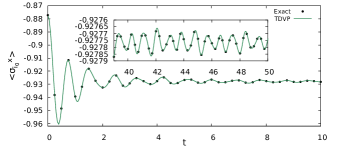
In Fig. 1, we show the transverse magnetization at site , , as a function of time, obtained both with mixed-iTDVP and the Ising exact solution.
As seen, the mixed-iTDVP works correctly well into the stationary regime.
Figure 1:
as a function of time, with = -1, , and , and .
The mixed-iTDVP computation is done with and .
The exact Ising solution is computed for an open chain with 512 sites.
The inset is from to 50.
VI.2 Effect of finite size
The defining feature of mixed-iTDVP is that it works directly in the thermodynamic limit.
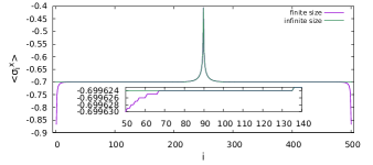
We demonstrate the lack of the finite size effect by computing the ground state of an inhomogeneous Hamiltonian: + with , and , where is in the middle of the chain.
The transverse magnetization of the ground state is shown in Fig. 2, in comparison with a finite size calculation with 500 sites.
Figure 2:
in the ground state of + with , and .
The calculation is done with .
The inset is a zoomed-in version of the main plot.
The curves for the finite system and the infinite system are overlapping for most times.
VI.3 speed of information spreading
Here we consider the spread of information after a local quench in the Ising chain both in the ballistic and the diffusive case.
In the ballistic case, the system is integrable and admits an extensive number of non-interacting quasi-particles in its spectrum, which transports energy ballistically.
When both and are non-zero, however, the Ising chain is no longer integrable, and the only locally conserved quantity is the energy.
In this case, there are no ballistically propagating quasi-particles so that, in an extended quantum quench, the energy is transported in a way similar to a random walk, at a speed which is proportional to Kim and Huse (2013).
This is called a diffusive system.
For the ballistic case, we take to be the with , , and .
For the diffusive case, we take to be the with , , and , which is shown to be robustly non-integrable in Kim and Huse (2013).
In both cases, the local quench is done through , where we place in the middle of the inhomogeneous region .
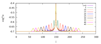
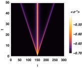
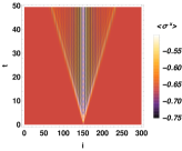
To monitor the spread of information, we measure the time dependence of on the whole chain, shown in Fig. 3(b) and 4.
The time dependence of other local observables are similar with .
Figure 3:
as a function of time, represented in a curve plot for both the ballistic system (top): = with , and , and the diffusive system (bottom): = with , = 0.9045, and = 0.8090.
The quenching Hamiltonian is in both cases.
The computation is done with and .
Computations with are also done, and the results are well-converged with the bond dimension.
(a)Ballistic system
(b)Diffusive system
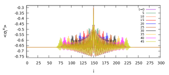
Figure 4:
as a function of time, represented in a contour plot, for the same two quenches described in Fig. 3(b).
Ballistic system
Diffusive system
A very sharp wave-front is observed in both cases as the information of the local quench spreads.
While this is expected for the ballistic system, it is surprising for the diffusive system, because the energy transports only diffusively in an extended quench.
The slope of the wave-front can be computed to give the speed of information spreading, .
More specifically, we do a linear fit of the function , which for the ballistic system equals the site of the left-most local maximum of at time , and take the slope of the linear fit as the slope of the wave-front.
For the diffusive system, we note that there exists a secondary peak in the magnetization profile, for example at around at = 45.
We take the to be the site on which is the largest in this secondary peak.
Table 2: Velocity of the wave-front in local quenches.
The number in the parenthesis is the uncertainty of the fit on the last digit.
is the -square of the linear fit.
system
ballistic
20
1.94(2)
0.99979
diffusive
20
1.71(3)
0.99949
Because of the discrete nature of , can be ambiguous up to .
This contributes to the slight non-linearity of , indicated by .
For the ballistic system, there are well-defined quasi-particles whose velocities are given by the dispersion relation: Kogut (1979).
One thus expects that the speed of information spreading should be
(22)
which equals 2 for all for the transverse-field Ising model.
This is very close to the velocity actually measured in the local quench.
The presence of the light-cone in the diffusive system, however, suggests that the ballistic spread of information is generic in a local quench, and happens not only in integrable systems.
VII Discussion
In this paper, we gave a detailed derivation of the TDVP equation for mixed infinite MPSs.
The result is a simple combination of the finite TDVP and infinite TDVP algorithms, both of which are inversion-free.
The method was applied to local quenches of the quantum Ising model, and interesting phenomenon were found, which calls for future work.
We also expect future work on the algorithmic side.
For example, we note that the mixed infinite MPS is very similar to the variational ansatz of the elementary excitations Vanderstraeten et al. (2019) of a translationally invariant system:
(23)
where labels the position of spin sites.
We thus hope that the current method can help develop a time-evolution algorithm for the elementary excitations.
Acknowledgements.
The code is based on ITensor ITe (version 3, C++), and is available upon request.
The author is grateful for the help received on the ITensor Support Q&A.
He is grateful for mentorship from his advisor Roberto Car at Princeton.
He acknowledges support from the DOE Award DE-SC0017865.
Before we start, we need some facts about the MPS transfer matrices and , defined as
(24)
We note that the canonical condition, Eq. 10, is the eigen-relation for the non-degenerate leading eigenvalue of the transfer operators, which is 1 for a normalized uniform MPS Vanderstraeten et al. (2019).
This is very important, because it means that if one propagates an arbitrary boundary tensor from left through infinitely many , only the leading left-eigvector of survives, which is a two-index delta tensor.
The analogous fact is true for , too.
We now determine the
that is the orthogonal projection of on the tangent space at .
To do this, we need to first compute the inner product , also known as the Gram matrix.
Using Eq. 10 and 12-15, we have:
To simplify further, we explicitly split out the contribution of from its leading eigenspace:
(25)
where is the leading left-eigenvector of , and is the contribution from the sub-leading eigenspace of .
Then,
(26)
This splitting is useful because has a spectral radius less than one, and the second term on the right-hand side of Eq. 26 converges.
We now have
(27)
where is a finite number.
Here we have used the normalization of the state:
(28)
An relation analogous to Eq. 27 holds for the tensors, too.
This gives the final form of the Gram matrix:
(29)
The Gram matrix is thus essentially diagonal in the effective parameters of .
We are ready to compute the orthogonal projection of , which is given by the solution to the minimization problem
is determined by
(30)
Here,
(31)
where the MPO transfer matrices , etc., are defined in Eq. 16.
In addition to their generalized eigenvectors, we denote the left eigenvectors of and right eigenvectors of respectively as and .
In fact, these eigenvectors do not depend on the values of the MPO, and thus are the same for and (see Appendix VIII.2).
As the left boundary tensor at left infinity propagates through infinitely many to meet the center site in Eq. 31, only the leading eigenspace survives.
The same applies to the right side.
Thus,
(32)
where
(33)
Here, and are two complex numbers.
They occur because every time passes through , there arises a new term of : , where is the energy density of the chain Zauner-Stauber et al. (2018).
Their values, however, do not matter because of the following lemmas.
Lemma VIII.1
.
(This lemma, and others below, are based on the Schur form of the MPO.
See Appendix VIII.2 for a discussion of their proofs.)
Lemma VIII.2
.
Thus,
As with , we split out of the term associated with the leading eigenspace.
To do this, we need the following lemma in linear algebra.
Lemma VIII.3
Let be a matrix with leading eigenvalue one, according to which there is one eigenvector and one generalized eigenvector.
Let be the left generalized eigenvector, the left eigenvector, the right eigenvector, and the right generalized eigenvector.
Then, for an integer ,
(34)
where is the contribution to from the sub-leading eigenspace.
When applying Lemma VIII.3 to , the contribution associated with the drops because of the following lemma.
Lemma VIII.4
(35)
Thus, we have
(36)
where we have made use of the following lemma.
Lemma VIII.5
(37)
where is the left eigenvector of .
Note that the second term of Eq. 36 converges.
Now substitute Eq. 36 into Eq. 30, and divide the equation by .
The finite terms drop, and we obtain Eq. 17.
Analogously, we obtain Eq. 18 and 19.
We now determine , which is given by
where
(38)
Here the and are the same as in Eq. 32.
Two lemmas are now in order:
Lemma VIII.6
.
Lemma VIII.7
Thus,
(39)
But note that gives a contribution of to , which can be dropped in the projective space.
Also recall that we still have one last gauge symmetry to spare, which we now use to demand so that in Eq. 20.
VIII.2 Schur form of MPO
As discussed in the main text, the matrix of an MPO is lower-triangular, known as the Schur form.
For example, in terms of the operator-valued matrices , the matrix of the transverse-field Ising Hamiltonian (when ) in Eq. 21 can be expressed as,
(40)
where and are the Pauli matrices.
To us, the important features of are that is lower triangular and that .
This means that the dominant left-eigenvector of and right-eigenvector of are
(41)
In addition, the generalized eigenvector and satisfy the following relation Zauner-Stauber et al. (2018):
(42)
We now discuss the proofs of the lemmas in Appendix VIII.1.
Lemma VIII.1: Because is non-zero only when its middle index is one, only contributes a to .
Thus, by Eq. 15.
Lemma VIII.2: Because is non-zero only when its middle index is , and that the only non-zero element in the column of is , the contributes only as .
This makes by Eq. 15.
Lemma VIII.3: This is proved by putting into its Jordan canonical form.
Lemma VIII.5: Because of the Schur form, is non-zero only when its middle index is 1, and is equal to in that case.
Then this lemma reduces to Eq. 28.
Lemma VIII.6: Because of the Schur form, is only non-zero when its middle index is 1, but is only non-zero when its middle index is .
This makes the whole thing zero.
Lemma VIII.7: Similar to Lemma VIII.2, contributes only as and contributes only as .
Thus, the whole expression reduces to .
VIII.3 Symplectic derivation of TDVP
The derivations Haegeman et al. (2011) of TDVP in the literature have been based on a variational principle, hence the name.
This has the benefit of not needing differential geometry, but buries the symplectic structure of TDVP under the heavy calculations in the derivation.
Here we give a derivation directly from symplectic geometry, which is quite elegant and may be preferable to a person who knows some basic differential geometry.
We assume knowledge of basic differential geometry at the level of chapter 5 and 8 of Nakahara (2003).
Let be a complex vector space with (complex) dimension .
can also be viewed as a real manifold with real dimension , and thus with a tangent space at of real dimension .
can be complexified to give which has complex dimension .
Let be a linear complex structure on .
and have two eigenvalues and , each with an eigenspace of complex dimension .
can then be written as a direct sum of the eigenspaces of : , where and .
Note that , and a linear isomorphism can be established: .
This allows one to extend the inner product of to :
(43)
Note that we do not define an inner product on .
allows a definition of a metric on : ,
(44)
This is known as the Hermitian metric.
It is such that for all .
defines a two-form :
(45)
(It is not hard to show .)
Because vector spaces are “flat”, does not change from point to point, thus .
This means is symplectic.
A manifold with a compatible complex structure , Hermitian structure , Riemannian structure , and symplectic structure is known as a Kähler manifold.
We have essentially shown that any complex vector space with an inner product is Kähler.
Let .
and are connected by the following:
(46)
On , for a Hamiltonian operator , consider the Hamiltonian flow of the Hamiltonian function .
For infinitesimal:
(47)
where is the Hamiltonian flow of :
(48)
This is nothing but the Schrödinger flow.
Thus, the Schrödinger dynamics can be viewed as a symplectic flow of the Hamiltonian function .
Now let be a submanifold of . Does induce a symplectic Schrödinger flow on ? Yes!
Let the inclusion function from to be denoted as
(49)
Both the Hamiltonian function and the symplectic form have a restriction on :
(50)
Because the exterior differentiation and the pullback commutes, , and thus is also symplectic.
We now look for the Hamiltonian flow associated with on .
For all , we look for such that .
(51)
Now here is the key, because are both only in , can be replaced with its orthogonal projection on , :
(52)
where is the Hamiltonian flow of on :
(53)
This gives the TDVP dynamics on and the dynamics is symplectic.
Haegeman et al. (2011)Jutho Haegeman, J. Ignacio Cirac, Tobias J. Osborne, Iztok Pivzorn, Henri Verschelde, and Frank Verstraete, “Time-dependent variational principle for quantum lattices,” Phys. Rev. Lett. 107, 070601 (2011).
Haegeman et al. (2016)Jutho Haegeman, Christian Lubich, Ivan Oseledets, Bart Vandereycken, and Frank Verstraete, “Unifying time evolution and optimization with matrix product states,” Phys. Rev. B 94, 165116 (2016).
Vidal (2007)G. Vidal, “Classical
simulation of infinite-size quantum lattice systems in one spatial
dimension,” Phys. Rev. Lett. 98, 070201 (2007).
Halimeh and Zauner-Stauber (2017)Jad C. Halimeh and Valentin Zauner-Stauber, “Dynamical phase diagram of quantum spin chains with long-range
interactions,” Phys. Rev. B 96, 134427 (2017).
Vanderstraeten et al. (2019)Laurens Vanderstraeten, Jutho Haegeman, and Frank Verstraete, “Tangent-space methods for uniform matrix product states,” SciPost Phys. Lect. Notes , 7 (2019).
Hastings (2010)Matthew B. Hastings, “Locality in quantum systems,” arXiv: Mathematical Physics (2010).
Milsted et al. (2013)Ashley Milsted, Jutho Haegeman, Tobias J. Osborne, and Frank Verstraete, “Variational
matrix product ansatz for nonuniform dynamics in the thermodynamic limit,” Phys. Rev. B 88, 155116 (2013).
Zauner-Stauber et al. (2018)V. Zauner-Stauber, L. Vanderstraeten, M. T. Fishman, F. Verstraete,
and J. Haegeman, “Variational optimization
algorithms for uniform matrix product states,” Phys.
Rev. B 97, 045145
(2018).
Michel and McCulloch (2010)Louis Michel and Ian P. McCulloch, “Schur forms
of matrix product operators in the infinite limit,” (2010).
Schollwöck (2011)Ulrich Schollwöck, “The
density-matrix renormalization group in the age of matrix product states,” Annals of Physics 326, 96 – 192 (2011), january 2011 Special Issue.
Young (1997)A. P. Young, “Finite-temperature and dynamical properties of the random transverse-field
ising spin chain,” Phys. Rev. B 56, 11691–11700 (1997).
Kim and Huse (2013)Hyungwon Kim and David A. Huse, “Ballistic spreading of entanglement in a diffusive nonintegrable system,” Phys. Rev. Lett. 111, 127205 (2013).
(17)ITensor Library (version
3.1.3).
Nakahara (2003)M. Nakahara, Geometry, topology
and physics (2003).