Epidemic plateau in critical SIR dynamics with non-trivial initial conditions

Abstract

Containment measures implemented by some countries to suppress the spread of COVID-19 have resulted in a slowdown of the epidemic characterized by time series of daily infections plateauing over extended periods of time. We prove that such a dynamical pattern is compatible with critical Susceptible-Infected-Removed (SIR) dynamics. In traditional analyses of the critical SIR model, the critical dynamical regime is started from a single infected node. The application of containment measures to an ongoing epidemic, however, has the effect to make the system enter in its critical regime with a number of infected individuals potentially large. We describe how such non-trivial starting conditions affect the critical behavior of the SIR model. We perform a theoretical and large-scale numerical investigation of the model. We show that the expected outbreak size is an increasing function of the initial number of infected individuals, while the expected duration of the outbreak is a non-monotonic function of the initial number of infected individuals. Also, we precisely characterize the magnitude of the fluctuations associated with the size and duration of the outbreak in critical SIR dynamics with non-trivial initial conditions. Far from heard immunity, fluctuations are much larger than average values, thus indicating that predictions of plateauing time series may be particularly challenging.

I Introduction

At the onset of the COVID-19 pandemic, world-wide time series of the number of infected individuals have displayed an exponential growth. Such a behavior is well predicted by standard epidemic frameworks Anderson et al. (1992). In slightly later stages, however, time series have exhibited non-trivial dynamical patterns. Many papers have attempted to model observed behaviors and to determine the role of containment measures Maslov and Goldenfeld (2020); Wong et al. (2020); Ferretti et al. (2020); Bianconi et al. (2020a); Fanelli and Piazza (2020); Carletti et al. (2020); Bianconi et al. (2020b); Bradde et al. (2020); Maheshwari and Albert (2020); Arenas et al. (2020); Ziff and Ziff (2020); Bianconi and Krapivsky (2020); Nekovee (2020); Valba et al. (2020); Blasius (2020); Brandenburg (2020). The common and reasonable assumption is that containment measures implemented in the attempt of mitigating the outbreak have strongly influenced the unfolding of the epidemic. Unfortunately, this a setting where modeling attempts are particularly challenging. The effective implementation of containment measures imposed by authorities rely on people’s personal judgements and adaptive behavior, and while epidemic spreading is a well-studied branch of mathematical biology Murray (2007), statistical physics Krapivsky et al. (2010) and network science Barabási et al. (2016); Newman (2010); Bianconi (2018); Barrat et al. (2008); Dorogovtsev (2010); Pastor-Satorras et al. (2015); Porter and Gleeson (2016), the modelling of adaptive behavior is only at its infancy Nanni et al. (2020); Gross et al. (2006); Gross and Sayama (2009).

According to the data, in several countries, the slowdown of the epidemic spread is characterized by an almost flat time series of daily number of new infections. Moreover, the time series of the number of removed individuals display power-law growth instead of an exponential growth as a function of time Ziff and Ziff (2020); Nekovee (2020); Blasius (2020); Brandenburg (2020). Here, we propose a theoretical interpretation of those features as the signature of the system being in (or near) its critical regime. Criticality is a fundamental property characterizing the dynamics of biological and socio-technical systems Mora and Bialek (2011); Munoz (2018); Gleeson and Durrett (2017). Our work consists of an in-depth investigation of a critical Susceptible-Infected-Removed (SIR) dynamics starting from a non-trivial initial configuration characterized by $n_{0}$ initially infected individuals. We interpret the emergence of the critical regime as the result of disease containment strategies, and the non-trivial initial condition as the configuration of the system when spreading becomes critical. In the typical setting considered in statistical mechanics Ben-Naim and Krapivsky (2004, 2012); Tomé and Ziff (2010), a single seed is generally used as the initial condition for critical SIR dynamics; the mapping of the critical SIR to the critical standard branching process allows for a full characterization of the spreading dynamics Zapperi et al. (1995); Lauritsen et al. (1996). The realistic assumption of having an initial number of infected individuals $n_{0}>1$ introduces an additional scale in the system affecting in a non-trivial manner the scaling properties of the SIR critical dynamics. While in other non-equilibrium systems a non-trivial initial condition may lead to a change of the critical exponent values Henkel et al. (2008); Janssen et al. (1989); Hinrichsen and Ódor (1998), in the critical SIR, the introduction of a non-trivial initial condition does not change the critical exponents that characterize the distribution of outbreak size and duration. However, it introduces lower exponential cutoffs in the distributions. As a result, the expected size and duration of the outbreak, as well as their standard deviations, have a non-trivial dependence on the initial condition $n_{0}$. In this paper, we evaluate, by means of analytic arguments and large-scale simulations, the scaling of these quantities as functions of the population size $N$.

The paper is structured as follows: in Section II, we provide the theoretical interpretation of the plateau as a critical SIR dynamics starting from $n_{0}>1$ initial condition; in Section III, we perform a statistical mechanics investigation of the statistical properties of the critical SIR dynamics with non-trivial initial conditions, supported by extensive numerical simulations of the process; finally, in Section IV, we provide concluding remarks. The Appendix describes the Gillespie algorithm used in this work to simulate the critical SIR dynamics.

II The theoretical interpretation of the plateau

We consider the Susceptible-Infected-Removed (SIR) model on a well-mixed population Krapivsky et al. (2010); Barabási et al. (2016); Newman (2010); Bianconi (2018); Barrat et al. (2008); Dorogovtsev (2010); Pastor-Satorras et al. (2015); Porter and Gleeson (2016). At any point in time, individuals can be found in three possible states: susceptible, infected and removed. Susceptible individuals do not carry the disease but they can be infected; infected individuals carry the disease, and they can spread it to susceptible individuals; removed individuals are either removed or deceased, and they do no participate in the spreading dynamics. We indicate with $\lambda$ the rate of infection, i.e., the expected number of spreading events occurring per unit of time. Without loss of generality, we set the recovery rate equal to one.

We start our discussion by focusing on the deterministic treatment of the SIR model on a well-mixed population with infinite size. If we indicate with $s$, $i$ and $r$ the fractions of susceptible, infected and removed individuals, respectively, we can write

$$\frac{ds}{dt} = -\lambda si,$$

$$\frac{di}{dt} = \lambda si-i,$$

$$\frac{dr}{dt} = i.$$ (1)

Please note that $s+i+r=1$. The critical dynamical regime is characterized by

$$\lambda_{c}=1\;.$$ (2)

If we start from an initial condition consisting of a fraction $i(0)$ of infected individuals and a fraction $r(0)=0$ of removed individuals, at the onset of the epidemic, i.e., $t\ll 1$, we observe a different behavior depending on the value of $\lambda$. In the non-critical regime, i.e., $\lambda\neq\lambda_{c}$, the deterministic equations for $i$ and $r$ read

$$\frac{di}{dt} = \lambda si-i\simeq(\lambda-1)i,$$

$$\frac{dr}{dt} = i.$$ (3)

Solutions of the above equations are

$$i(t)=i(0)e^{(\lambda-1)t},$$

$$r(t)=\frac{i(0)}{\lambda-1}e^{(\lambda-1)t}.$$ (4)

In essence, in the subcritical regime, i.e., $\lambda<\lambda_{c}$, the number of infected individuals decays exponentially fast, and the number of removed individuals remains vanishing. In the supercritical regime, i.e., $\lambda>\lambda_{c}$, the number of infected and removed individuals displays an exponential increase. At criticality, i.e., $\lambda=\lambda_{c}$, the deterministic equations for $i$ and $r$ are

$$\frac{di}{dt} = (s-1)i\ll 1,$$

$$\frac{dr}{dt} = i\;,$$ (5)

leading to

$$i(t)\simeq i(0),$$

$$r(t)\simeq i(0)t.$$ (6)

Therefore, according to the deterministic approach, for small times we should expect that the number of removed individuals at criticality increases linearly in time with a slope that is given by the initial condition $i(0)$, at the onset of the epidemics.

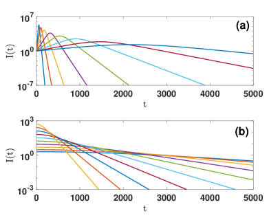
Figure 1: a) Time series of the number of infected individuals $I(t)=i(t)\,N$ are plotted close to the critical point. $I(t)$ correspond to the solution of the deterministic SIR equations. The population size is $N=10^{7}$, and spreading is started from $n_{0}=1$ seed. Different curves correspond to different values of $\lambda=1+2^{-q}$, with $q=2,3,4,\ldots,8,9$. b) Same as in panel a, but for $\lambda=1$. Different curves correspond to different numbers of initially infected nodes $n_{0}=2^{q}$, with $q=2,3,4,\ldots,8,9$. As $\lambda$ approaches the critical value $\lambda_{c}=1$ and $n_{0}$ decreases toward one, we observe a plateauing of the time series.

From the deterministic Eqs. (1), it is evident that

$$\frac{di}{ds}=-1+\frac{1}{\lambda s}.$$ (7)

The equation can be integrated to obtain the well-known solution Krapivsky et al. (2010)

$$s(t)+i(t)-\frac{1}{\lambda}\ln s(t)=s(0)+i(0)-\frac{1}{\lambda}\ln s(0).$$ (8)

Using Eqs.(1), we can express the logarithmic derivative of the number of infected individuals as

$$\frac{d\ln i}{dt}=\lambda s-1,$$ (9)

where $\lambda\,s(t)$ is the reproduction number.

The former equation implies that the time series of infected individuals $i(t)$ has a peak at $t=t^{\star}$ determined by

$$\lambda s(t^{\star})=1.$$ (10)

The fraction of susceptible individuals at the peak of the epidemic is given by $s^{\star}=s(t^{\star})=1/\lambda$. By making the further assumption that the epidemic starts from a fraction $i(0)=1-s(0)$ of infected individuals and zero removed individuals $r(0)=0$ in Eq. (8), we obtain

$$i^{\star}=i(t^{\star})=1-\frac{1}{\lambda}-\frac{1}{\lambda}\ln(\lambda s(0)).$$ (11)

Using Eqs. (10) and (11) in the first of Eqs. (1), we get

$$\left.\frac{ds}{dt}\right|_{t=t^{\star}}=-\lambda s^{\star}i^{\star}=-i^{\star}$$ (12)

It follows that the second derivative of $\ln i$ is given by

$$\left.\frac{d^{2}i}{dt^{2}}\right|_{t=t^{\star}}=i(t^{\star})\left.\frac{d^{2}\ln i}{dt^{2}}\right|_{t=t^{\star}}=-\lambda(i^{\star})^{2}=-\rho^{\star},$$ (13)

where $\rho^{\star}$ is defined as

$$\rho^{\star}=-\frac{1}{\lambda}\left(\lambda-1-\ln(\lambda s(0))\right)^{2}.$$ (14)

We note that $\rho^{\star}$ is zero, i.e., we reach a plateau, only for $s(0)=1$ and $\lambda=1$. This fact implies that, in the deterministic approach, a perfect plateau of the time series $\ln i$ is never achieved for $\lambda>1$.

In the vicinity of the critical point, the time series of the infected individuals is still well described by a plateau. Developing the right-hand side of Eq. (13) around $\lambda=1$, $s(0)=1$, we get $s(0)\simeq 1$ and

$$\rho^{\star} \simeq -\frac{1}{\lambda}\left[\ln(s(0))+\frac{1}{2}(\lambda-1)^{2}\right]^{2}$$ (15)

$$\simeq \left[1-s(0)+\frac{1}{2}(\lambda-1)^{2}\right]^{2}.$$

The above equation indicates that the conditions to have a near-plateau dynamics are having an infectivity rate $\lambda$ close to one, and having the system as far as possible from heard immunity, i.e., $1-s(0)\ll 1$. In summary, the near-critical state for $\lambda\simeq 1$ is a fragile state that can be characterized by a very slow dynamics if containment measures do not further decrease the infectivity $\lambda$ below one (see Figure 1).

III SIR critical dynamics with non-trivial initial condition

From now on, we assume that the system is in the critical regime. We further assume that spreading dynamics is started from $n_{0}>1$ initial seeds. The two assumptions serve to rationalize two main features of real time series. First, time series are characterized by long temporal windows of almost flat behavior. This is a signature of criticality. Second, plateaus are observed only after initial growths in the number of infected individuals, meaning that the critical regime is reached only after that containment strategies have effectively changed the spreading dynamics of the disease. Whereas critical properties of the SIR model are well understood for spreading processes initiated by $n_{0}=1$ individual, we are not aware of existing studies dealing with non-trivial initial conditions consisting of $n_{0}>1$ seeds. How do the properties of the critical dynamics change with $n_{0}$? What is the behavior of the expected duration of the outbreak? What about the expected size of the outbreak? What about their fluctuations?

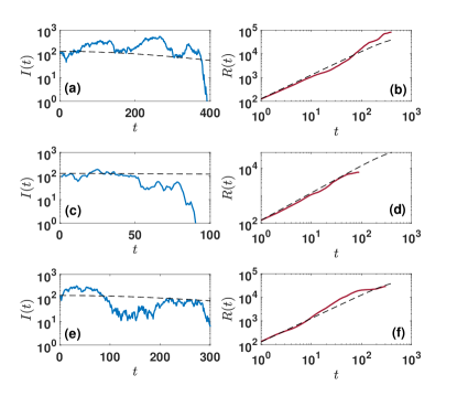
Figure 2: We show three examples of time series for the number of infected individuals $I(t)$ (panels a, c and e) and the corresponding number of removed individuals $R(t)$ (panels b, d and f) for a critical SIR dynamics with non-trivial initial condition. The time series are obtained by simulating the stochastic SIR dynamics at criticality (with $\lambda=1$) on a well-mixed population with identical parameters: initial number of infected individuals $n_{0}=128$ and population size $N=10^{7}$. The dashed lines indicate the corresponding deterministic predictions.

Please note that all the above questions cannot be answered with a purely deterministic approach. SIR outbreak sizes and durations obey probability distributions that are well peaked around their expected value only if the system is off criticality. However, the very fact that the system is assumed to be in the critical regime implies that fluctuations have a dominant role in the determination of the properties of the dynamical system. In Figure 2 for example, we display time series representative for the critical regime of the dynamics. Ground-truth time series are obtained by simulating the SIR stochastic dynamics (see Appendix A for details). They are compared with the deterministic expectation value obtained by integrating Eqs. (1). We note that some realizations of the process are more persistent and more pervasive in the population than what predicted by the expected value.

From here on, we abandon the deterministic SIR equations and we embrace a stochastic approach. Critical SIR dynamics starting from a single initial seed, i.e., $n_{0}=1$, is known to be characterized by extremely large fluctuations of the outbreak size and duration. These fluctuations can be quantified by leveraging the mapping between critical SIR in a well-mixed population and the mean-field branching process. In the following sections, we first review results valid for $n_{0}=1$. Then, we focus our attention on the non-trivial case $n_{0}>1$.

III.1 Critical dynamics with $n_{0}=1$ initial seed

If the initial condition is such that only one node is in the infected state while all other nodes are in the susceptible state, the critical SIR model gives rise to outbreaks that follow the statistics of a critical branching process Zapperi et al. (1995); Lauritsen et al. (1996) corrected by some scaling functions $F_{T}(N/N_{T}^{\star})$ and $F_{R}(N/N_{R}^{\star})$ that implement the effective cutoff caused by finite-size effects Ben-Naim and Krapivsky (2004, 2012). Here, $N$ is the size of the system; $N_{T}^{\star}$ and $N_{R}^{\star}$ are instead parameters that determine when the cutoff takes place. Specifically, the distribution $P(T)$ of the duration $T$ of an outbreak follows the law

$$P(T)\sim T^{-2}F_{T}(N/N_{T}^{\star}),$$ (16)

while the size of the outbreak $R$ follows the distribution

$$P(R)\sim R^{-3/2}F_{R}(N/N_{R}^{\star}).$$ (17)

The cutoff sizes $N_{T}^{\star}$ and $N_{R}^{\star}$ have been derived in Refs. Ben-Naim and Krapivsky (2004, 2012). They are given by

$$N_{T}^{\star}=T^{3}, N_{R}^{\star}=R^{3/2}.$$ (18)

From the expressions for $P(T)$ and $P(R)$ given by Eqs. (16) and (17), respectively, and further assuming a sharp cutoff, it is easy to deduce that the scaling with the system size $N$ of the average outbreak size $\langle{R}\rangle$, the average duration $\langle{T}\rangle$, and the standard deviations $\sigma_{R}$ and $\sigma_{T}$ Ben-Naim and Krapivsky (2004, 2012) obey

$$\langle{R}\rangle\sim N^{1/3}, \sigma_{R}\sim N^{1/2},$$

$$\langle{T}\rangle\sim\ln N, \sigma_{T}\sim N^{1/6}.$$ (19)

We observe that all the above quantities are sub-extensive, as they all grow sub-linearly with the system size. The expected critical outbreak size $\langle{R}\rangle$ grows as the system size to the power of $1/3$. However, the standard deviation associated to the outbreak size, i.e., $\sigma_{R}$, grows with increasing system size much faster than $\langle{R}\rangle$. This fact indicates that it is very challenging to make predictions if the dynamics is critical. Similarly, the outbreak duration is characterized by large fluctuations in the large population limit. We note that the exponents $2$ and $3/2$ of the distribution $P(T)$ and $P(R)$ are the critical mean-field exponents. These exponents are universal and are observed for many critical spreading processes Radicchi et al. (2020). They characterize the critical SIR on network topologies too as long as the underlying network has a homogeneous degree distribution. In power-law networks, these exponents can deviate from their mean-field values as investigated in Refs. Goh et al. (2003); Radicchi et al. (2020).

We have seen in Section II that the deterministic approach predicts a linear increase of the number of removed individuals with time for small time. However, such a prediction is not accurate for the ground-truth dynamics; accounting for stochastic effects correctly predicts a quadratic growth of the number of removed individuals in time when the epidemic starts with a single initial seed. To this end, the number of removed individuals grows in time as a power law

$$R=\overline{t}^{z},$$ (20)

where $z$ is a dynamical critical exponent, and $\overline{t}$ is the expectation value of the time necessary to observe $R$ removed individuals. The value of the dynamical critical exponent can be obtained in different ways Lauritsen et al. (1996). Here, we present the derivation of the value of the dynamical exponent based on Langevin-like equations for the dynamics. Starting from an initial fraction of infected individuals $i(0)=n_{0}/N$ and a fraction $r(0)=0$ of removed individuals we write

$$\frac{di}{dt} = (\lambda s-1)i+c\sqrt{i}\eta(t),$$

$$\frac{dr}{dt} = i,$$ (21)

where $\eta(t)$ is an uncorrelated white noise with $\mathbb{E}({\eta(t)})=0$ and $\mathbb{E}(\eta(t)\eta(t^{\prime}))=\delta(t-t^{\prime})$ and $c$ is a constant. At criticality, i.e., $\lambda=\lambda_{c}=1$, thus, assuming $t\ll 1$ and $i(0)\ll 1$, we have $\lambda s-1\simeq-i(0)$. We can therefore write

$$\frac{di}{dt} = c\sqrt{i}\eta(t),$$

$$\frac{dr}{dt} = i.$$ (22)

We now perform a simple scaling analysis of this stochastic equations as usually done in non-equilibrium statistical mechanics, e.g., Refs. Barabási and Stanley (1995); Henkel et al. (2008); Marro and Dickman (2005). If we rescale time as

$$t\to bt$$ (23)

and define the scaling exponents $z,\alpha,$ for $r,i$

$$r \to b^{z}t,$$

$$i \to b^{\alpha}t,$$ (24)

as the exponents that leave the SIR critical dynamics unchanged. The SIR stochastic Eqs. (22) read

$$b^{\alpha-1}\frac{di}{dt} = cb^{\alpha/2-1/2}\eta(t),$$

$$b^{z-1}\frac{dr}{dt} = b^{\alpha}i,$$ (26)

from which we can derive the scaling exponents

$$\alpha = 1$$ (27)

$$z = 2.$$ (28)

In summary, in the critical dynamical regime, if the spreading is started from a single initial seed, we expect that the average number of removed individuals grows quadratically with time.

III.2 Critical dynamics with $n_{0}>1$ initial seeds

Critical SIR dynamics started from the non-trivial initial condition $n_{0}>1$ differs from the critical SIR dynamics started from $n_{0}=1$ seed. To include an explicit dependence on the parameter $n_{0}$ in the scaling of Eq. (20), we correct it by introducing the scaling function $F(x)$, where $x=n_{0}/\overline{t}(R)$. We impose that

$$R\simeq\overline{t}(R)^{z}F\left(\frac{n_{0}}{\overline{t}(R)}\right)$$ (29)

with

$$F(u)\sim\left\{\begin{array}[]{ccc}1&\mbox{if}&u\gg 1\\ u^{\beta}&\mbox{if}&u\ll 1\end{array}\right.$$ (32)

According to the deterministic SIR equations for $t\ll 1$ and $i(0)\ll 1$, the number of removed individuals grows linearly in time with a slope $i(0)=n_{0}/N$. Thus, we deduce that

$$\beta=1.$$ (33)

This value is well supported by extensive numerical results (see Figure 3) which confirm that there is a cross-over between linear and quadratic dependence of $R$ on $\overline{t}(R)$.

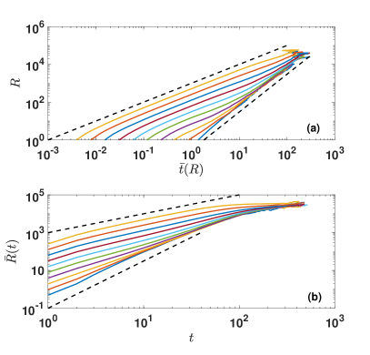
Figure 3: Dynamical properties of the critical SIR process with non-trivial initial condition. a) We plot the number of removed individuals $R$ versus the expected time $\bar{t}(R)$ required to observe $R$ removed individuals. The different curves indicate different initial conditions, from bottom to top, $n_{0}=2^{q}$, with $q=2,3,4,\ldots,8,9$. The population size is $N=10^{7}$. The dashed lines are guides to the eye and correspond to linear and quadratic growth of $R$ versus $\bar{t}(R)$, respectively. b) Expected number $\bar{R}(t)$ of removed individuals as a function of time $t$. Data are the same as in panel a. The dashed lines are guides to the eye and correspond to power-law growth of $\bar{R}$ versus $t$ with exponent $\xi=1$ and $\xi=2.5$, respectively.

In the simulation of the SIR model, it is natural to study the behavior of $R$ as a function of $\overline{t}(R)$. However, in real epidemic time series, the number of infected individuals is measured over constant time intervals. The two ways of monitoring the evolution of the process, i.e., $R$ versus $\overline{t}(R)$ rather than $\overline{R}(t)$ versus time $t$, may lead to the observation of different scaling exponents. The discrepancy is due to the stochastic nature of the spreading process. The phenomenon is apparent from the results of Figure 3: depending on the type of measurement performed on the system, the power-law increase of the number of removed individuals as a function of time can be described by a continuous range of exponents ranging from $\xi=1$ to $\xi\sim 2.5$. We can therefore write

$$\overline{R}(t)\simeq n_{0}t^{\xi}h(t,N)$$ (34)

where $\xi$ is a decreasing function of $n_{0}$, and $h(t,N)$ is a modulating function expressing the deviation from the pure power-law behavior. The ansatz of the above equation is compatible with the power-law scaling of the empirical time series of removed individuals as a function of time observed in countries where containment measures have been implemented extensively Ziff and Ziff (2020); Nekovee (2020); Blasius (2020); Brandenburg (2020).

III.3 Distribution of avalanche durations and sizes for the critical SIR model initiated by $n_{0}>1$ seeds

In this section we investigate the statistical properties of the distribution of outbreak duration and size for the critical SIR dynamics in a well mixed-population when the initial condition is non-trivial, i.e., $n_{0}>1$. Scaling arguments suggest the following expression for the distribution $P(T)$ of the critical outbreak duration $T$

$$P(T)\sim n_{0}T^{-2}{F}_{T}(N/N_{T}^{\star},n_{0}/T).$$ (35)

The above scaling function is a natural modification of Eq. (16) by assuming that $n_{0}$ scales like time. In particular, the distribution $P(T)$ is characterized by a lower cutoff depending on $n_{0}$. This fact is intuitive as an outbreak with a larger number of initially infected individuals is not expected to reach the absorbing state faster than an outbreak started by a single seed (see Figure 4a). We note that, in the critical SIR dynamics, the dependence on $n_{0}$ does not lead to a change of the critical exponent values, as for example observed in other non-equilibrium phase transitions Janssen et al. (1989); Henkel et al. (2008); Hinrichsen and Ódor (1998). In Figure $\ref{fig:w}a$, we display the function

$$w_{T}(n_{0},T)=-\ln\frac{{F}_{T}(N/N_{T}^{\star},n_{0}/T)}{{F}_{T}(N/N_{T}^{\star},1/T)}$$ (36)

and we demonstrate that the scaling function $w_{T}(n_{0}/T)$ for $n_{0}\ll N_{T}^{\star}$ can be approximated as

$${w}_{T}(n_{0},T)\simeq-\frac{n_{0}-1}{T}.$$ (37)

The scaling behavior, valid for $n_{0}\ll N^{1/3}$, can be justified by assuming that each of the $n_{0}$ seeds generates an independent outbreak obeying the statistics of the critical branching process. A critical avalanche started from a single infected individual has a duration $T$ following the power-law distribution $\pi(T)\sim T^{-2}$ Zapperi et al. (1995); Lauritsen et al. (1996). Thus, assuming independence among the $n_{0}$ avalanches, we can estimate the probability $P(T)$ as the probability that among all $n_{0}$ outbreaks the last outbreak to get extinguished is extinguished at time $T$. Therefore in the infinite population limit we obtain

$$P(T)\simeq n_{0}[1-\pi_{c}(T)]^{n_{0}-1}\pi(T),$$ (38)

where $\pi_{c}(T)$ is the probability that an outbreak generated by a single infected individual is not extinguished at time $T$, with $\pi_{c}(T)\int_{T}^{\infty}\pi(x)dx\simeq{1}/{T}$. By assuming $1\ll n_{0}\ll N^{1/3}$, we get

$$P(T)\simeq n_{0}\exp\left(-\frac{n_{0}-1}{T}\right).$$ (39)

Finally, we note that while the scaling behavior described in Eq. (37) has strong numerical confirmation for $T\ll N_{T}^{\star}$ for values of $T\sim N_{T}^{\star}$ the scaling function $w_{T}(n_{0},T)$ signals a dependence of the cutoff on $n_{0}$ (see Figure 5).

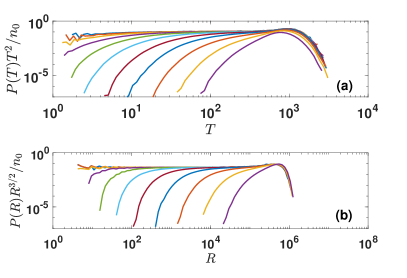
Figure 4: The rescaled distribution of outbreak duration $P(T)$ (panel a) and outbreak size $P(R)$ (panel b) are plotted for a well-mixed population of $N=10^{8}$ individuals and initial number of infected individuals $n_{0}$ equal to $2^{q}$, with $q=2,3,4,\ldots,10,11$. The distributions display a lower cutoff that increases as $n_{0}$ increases, and an upper cutoff whose value does not strongly depend on $n_{0}$.

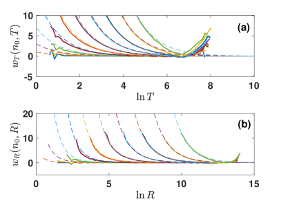
Figure 5: The function $w_{T}(n_{0},T)$ and $w_{R}(n_{0},R)$ defined in Eq. (36) (panel a) and Eq. (41) (panel b) are plotted for a population of $N=10^{8}$ individuals and different values of $n_{0}=2^{q}$, with $q=2,3,4,\ldots,10,11$. The dashed lines correspond to the scaling expressed in Eq. (37) and Eq. (42).

Scaling arguments suggest that the distribution $P(R)$ of critical outbreak size $R$ should obey

$$P(R)\sim n_{0}R^{-3/2}F_{R}(N/N_{R}^{\star},n_{0},R),$$ (40)

where the function $F_{R}(N/N_{R}^{\star},n_{0},R)$ implements a lower cutoff dependent exponentially on $n_{0}$ (see Figure 4b).

In Figure $\ref{fig:w}b$, we show the function

$$w_{R}(n_{0},R)=-\ln\frac{{F}_{R}(N/N_{R}^{\star},n_{0},R)}{{F}_{R}(N/N_{R}^{\star},1,R)}$$ (41)

which, for $n_{0}\ll N_{R}^{\star}(R,n_{0})$, can be approximated as

$${w}_{R}(n_{0},R)\simeq-\frac{n_{0}^{2}}{R}-\frac{n_{0}^{5/2}}{R^{2}}.$$ (42)

This scaling function indicates that, for large values of $R$, $R$ scales like $n_{0}^{2}$. For small values of $R$, it is possible to observe some corrections would be required to fully describe the scaling. We notice that, in the first order in $n_{0}$, the normalization constant of the distribution $P(R)$ is independent of $n_{0}$. A way to interpret the result is by considering the infinite population limit approximating the distribution $P(R)$ as the convolution of the $n_{0}$ sizes of independent outbreak events. In this limit we have

$$P(R)=\int d\omega e^{i\omega R}\left[\mathcal{F}(\omega)\right]^{n_{0}},$$ (43)

where $\mathcal{F}(\omega)=\sum_{r}\Pi(r)e^{-i\omega r}$ is the generating function of the distribution $\Pi(r)$ of avalanches sizes of SIR critical dynamics starting from a single seed. Assuming in first approximation that $\Pi(r)$ is a pure power law $\Pi(r)\sim r^{-3/2}$, it follows that the logarithm of the generating function behaves, for small $\omega$, as $\ln\mathcal{F}(\omega)\sim\sqrt{\omega}$. The result, together with Eq. (43), indicates that $R$ should scale as $n_{0}^{2}$ for $n_{0}\ll N^{2/3}$. For mor details on the infinite population limit we refer the reader to Ref. Krapivsky (2020).

III.4 Statistical properties of the critical outbreak started by $n_{0}>1$ seeds

III.4.1 General scenario

We performed large-scale simulations of the critical SIR model to address fundamental questions regarding the distributions of duration $T$ and size $R$ of outbreaks started by a non-trivial initial condition $n_{0}>1$. In Figure 6, we display the average values and the standard deviations of both $T$ and $R$ for a large system composed of $N=10^{8}$ individuals. We display the moments of the distributions as a function of the number of initial seeds $n_{0}$. The main outcomes are as follows. The expected size $\langle{R}\rangle$ is a growing function of $n_{0}$. The expected duration $\langle{T}\rangle$ is a non-monotonic function of $n_{0}$, displaying a single peak. The standard deviations $\sigma_{T}$ and $\sigma_{R}$ also display a peak as a function of $n_{0}$. The coefficient of variation $\sigma_{T}/\langle{T}\rangle$ and $\sigma_{R}/\langle{R}\rangle$ are monotonically decreasing with $n_{0}$. We conclude that fluctuations are fundamental to properly characterize the critical dynamical regime. This statement is true for any value of $n_{0}$, albeit, in relative terms, the most severe effect of fluctuations is observed for $n_{0}=1$. We note that as the initial number of infected individuals $n_{0}$ increases, the expected size of the outbreak displays a monotonic increase while the expected duration of the outbreak displays a maximum. In the following subsection, we will provide scaling laws for these major statistical properties of the critical dynamics as a function of the number of initially infected individuals.

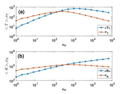
Figure 6: a) The expected value of the duration of critical outbreak $\langle{T}\rangle$ and the corresponding standard deviation $\sigma_{T}$ are plotted versus the number $n_{0}$ of individuals initially infected. The population size is $N=10^{8}$. Results are obtained relying on $10^{4}$ independent realizations of the process. b) The expected size of the critical outbreak $\langle{R}\rangle$ and the corresponding standard deviation $\sigma_{R}$ are plotted versus the number $n_{0}$ of individuals initially infected. Data are the same as of panel a.

III.4.2 Scaling analysis of $\langle{T}\rangle$ and $\sigma_{T}$

We make the ansatz that the average duration $\langle{T}\rangle$ can be described by

$$\langle{T}\rangle \simeq G(n_{0}|\alpha,\beta,H,K),$$ (44)

where the function $G(n_{0}|\alpha,\beta,H,K)$ is given by

$$G(n_{0}|\alpha,\beta,H,K)=\frac{n_{0}^{\alpha}H}{1+n_{0}^{\beta}K}.$$ (45)

Here, $\alpha$ and $\beta$ are, in the large population limit, independent of $N$. On the contrary, $H$ and $K$ are dependent on the population size. By introducing the function

$$g(x|\alpha,\beta)=\frac{x^{\alpha}}{1+x^{\beta}},$$ (46)

we observe that it is possible to rescale the curves obtained for different values of $N$ by performing the transformation

$$H^{-1}K^{\alpha/\beta}G(n_{0}|\alpha,\beta,H,K)=g(n_{0}K^{1/\beta}|\alpha,\beta).$$ (47)

This expression allows us to perform a data collapse of the data obtained for $\langle{T}\rangle$ at different values of $n_{0}$ and different population size $N$ (see Figure 7a).

We observe that, if we start from a non-trivial initial condition $n_{0}$, the expected duration of the outbreak $\langle{T}\rangle$ reaches its maximum at

$$n_{0}^{\star}=\left(\frac{\alpha}{K(\beta-\alpha)}\right)^{1/\beta}.$$ (48)

The scaling parameters $H$ and $K$ obey the scaling relation

$$K\simeq a_{K}N^{\delta_{K}}, H\simeq a_{H}\log(N)+b_{H}.$$ (49)

with $a_{H}=0.58\pm 0.08$, $b_{H}=-2.0\pm 0.9$, $\delta_{K}=-0.37\pm 0.04$ and $a_{K}=0.75\pm 0.06$ (see Figure 9). We note that the logarithmic scaling of $H$ is expected from the known scaling of $\langle{T}\rangle$ for the SIR critical model starting from a single initial seed. The exponents $\alpha$ and $\beta$ are given by

$$\alpha=0.78\pm 0.03, \beta=1.10\pm 0.1.$$ (50)

The standard deviation of the outbreak duration $\sigma_{T}$ can be described in the same exact way as $\langle{T}\rangle$. The ansatz

$$\sigma_{T} \simeq G(n_{0}|\alpha,\beta,H,K),$$ (51)

leads to the data collapse shown in Figure 7b. The scaling parameters $H$ and $K$ obey the scaling relations

$$K\simeq a_{K}N^{\delta_{K}}, H\simeq a_{H}N^{\delta_{H}}.$$ (52)

with $\delta_{H}=0.17\pm 0.01$, $b_{H}=1.7\pm 0.2$, $\delta_{K}=-0.36\pm 0.03$ and $a_{K}=2.3\pm 0.7$ (see Figure 9). We note that $\delta_{H}\simeq 1/6$. Therefore, for $n_{0}=1$ the scaling reduces to the well-known scaling for the critical SIR model starting from a single initial seed. Moreover, the exponent $\alpha$ and $\beta$ for $\sigma_{T}$ are given by

$$\alpha=0.50\pm 0.05, \beta=1.0\pm 0.1.$$ (53)

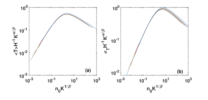
Figure 7: Finite-size scaling analysis for the duration $T$ of the critical SIR started from $n_{0}$ initial seeds. a) Data describing the average value of the outbreak duration $\langle{T}\rangle$ for different system sizes $N$ are collapsed on a unique universal curve using the scaling of Eq. (47). Data are shown for population sizes $N$ ranging from $N=10^{5}$ to $10^{8}$. Each data point is obtained by simulating the SIR process $10^{4}$ times. b) Same as in panel a, but for the standard deviation $\sigma_{T}$.

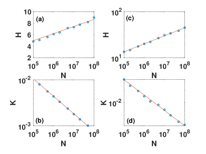
Figure 8: a) Scaling parameter $H$ as a function of the system size $N$ for the average duration $\langle{T}\rangle$ of critical outbreaks. Data points are the same as those of Figure 7. The line displays the best fit of the data points with Eq. (49). b) Same as in panel a, but for the scaling parameter $K$. c) Same as in panel a, but for the standard deviation $\sigma_{T}$. The orange line is the best fit of the data points with Eq. (52). d) Same as in panel c, but for the scaling parameter $K$.

Figure 9: a) The fitting parameter $\gamma$, i.e., Eq.(54), as a function of the system size $N$. Data points are the same as those of Figure 7. The line displays the best fit of the data points with Eq. (57). b) Scaling parameter $H$ as a function of the system size $N$ for the standard deviation $\sigma_{R}$ of critical outbreaks. The solid line corresponds to the scaling function of Eq.(62). c) Same as in panel b, but for the scaling parameter $K$. The solid line corresponds to the scaling function of Eq.(62).

III.4.3 Scaling analysis of $\langle{R}\rangle$ and $\sigma_{R}$

The ansatz for $\langle{R}\rangle$ is slightly different from the one appearing in Eq. (45), as it includes an additional logarithmic correction

$$\langle{R}\rangle \simeq \frac{n_{0}^{\alpha}H}{1+n_{0}^{\beta}(\ln n_{0})^{\gamma}K}.$$ (54)

We take

$$H=\frac{3}{2}N^{1/3}, K=N^{-1/3}$$ (55)

and

$$\alpha=1, \beta=0.5.$$ (56)

and we perform a fit of the exponent $\gamma$. As Figure 9a and Figure 10a demonstrate, the function gives rise to excellent data fits as long as the exponent $\gamma$ is

$$\gamma=a_{\gamma}\ln N+b_{\gamma}$$ (57)

with $a_{\gamma}=0.053\pm 0.003$ and $b_{\gamma}=0.30\pm 0.06$.

The function $\langle{R}\rangle$ can be rescaled and the data obtained for different $N$ collapsed on a universal curve (see Figure 10). This task is done by noting that

$$\langle{R}\rangle y(n_{0})=g(x(n_{0})|\alpha,\beta),$$ (58)

where

$$x(n_{0}) = n_{0}(\ln n_{0})^{\gamma/\beta}K^{1/\beta},$$

$$y(n_{0}) = H^{-1}K^{\alpha/\beta}(\ln n_{0})^{\alpha\gamma/\beta},$$ (59)

and the function $g(x|\alpha,\beta)$ is given by Eq. (46). The expected size of the outbreak $\langle{R}\rangle$ does not display a maximum as a function of $n_{0}$, i.e., it is a monotonous increasing function of $n_{0}$. The standard deviation $\sigma_{R}$ can be instead fitted using the same ansatz as $\sigma_{T}$, i.e.,

$$\sigma_{R} \simeq G(n_{0}|\alpha,\beta,H,K).$$ (60)

The best estimates of the parameters are

$$\alpha=0.57\pm 0.03, \beta=0.95\pm 0.05,$$ (61)

and

$$K\simeq a_{K}N^{\delta_{K}}, H\simeq a_{H}N^{\delta_{H}}.$$ (62)

with $\delta_{H}=0.48\pm 0.02$, $b_{H}=1.8\pm 0.5$, $\delta_{K}=-0.25\pm 0.03$ and $a_{K}=0.49\pm 0.3$ (see Figure 9). The corresponding data collapse is shown in Figure 10b.

Figure 10: Finite-size scaling analysis for the size $R$ of the critical SIR started from $n_{0}$ initial seeds. a) Data describing the average value of the outbreak size $\langle{R}\rangle$ for different system sizes $N$ are collapsed on a unique universal curve using the scaling of Eq. (58). Data are the same as of Figure 7. b) Same as in panel a, but for the standard deviation $\sigma_{R}$.

IV Conclusions

Motivated by the current COVID-19 pandemic, we have investigated the critical properties of the Susceptible-Infected-Removed (SIR) dynamics in well-mixed populations starting from non-trivial initial conditions consisting of $n_{0}>1$ infected individuals. Although the modeling framework oversimplifies the real-world scenario, the setting is realistic in two main respects. First, the plateauing time series observed in empirical data are compatible with the critical dynamical regime. Second, the initial condition $n_{0}>1$ is representative for a critical regime reached, thanks to effective containment measures, after that a significant community transmission already took place. We have shown that a non-trivial initial condition $n_{0}>1$ introduces another typical scale on the dynamics inducing a lower cutoff in the distributions of the duration and size of critical outbreaks. The critical dynamics is characterized by very strong fluctuations, but the presence of a non-trivial initial condition mitigates the role of the fluctuations. In particular, while for a single initial seed the standard deviation on the outbreak size and duration is much larger than the corresponding expectation values, the relative error diminishes as the size $n_{0}$ of the initial seed set increases. Moreover, numerical results indicate that, as the initial number of infected individuals $n_{0}$ increases, the expected size of the outbreak increases while the expected duration first increases and then decreases, displaying a maximum. Using scaling arguments, and extensive numerical simulations we have deduced the scaling of the maximum duration and the corresponding number of initially infected individuals.

Appendix A Stochastic SIR dynamics on well mixed populations

The critical SIR dynamics in a well-mixed population of $N$ individuals is simulated with the following implementation of the Gillespie algorithm Gillespie (1976). We indicate with $S(t),I(t)$ and $R(t)$ respectively the number of susceptible, infected and removed individuals as a function of time $t$. We start from the initial condition of $I(0)=n_{0}$, $S(0)=N-n_{0}$ and $R(0)=0$. At each elementary step, the algorithm proceeds as follows:

• Time increases by the amount $\Delta t$

  $$t\to t+\Delta t,$$ (63)

  where $\Delta t$ is given by

  $$\Delta t=\frac{-\log(q)}{\lambda S(t)I(t)+I(t)}.$$ (64)

  with $q\sim\textrm{Unif.(0,1)}$, i.e., a random variate extracted from the uniform distribution in the domain $(0,1)$.

• With probability

  $$p=\frac{\lambda S(t)I(t)}{\lambda S(t)I(t)+I(t)}$$ (65)

  a susceptible individual becomes infected, i.e.,

  $$S(t+\Delta t) = S(t)-1,$$

  $$I(t+\Delta t) = I(t)+1.$$ (66)

• With probability $1-p$ an infected individual is removed, i.e.,

  $$I(t+\Delta t) = I(t)-1,$$

  $$R(t+\Delta t) = R(t)+1.$$ (67)

The critical dynamics is obtained by setting $\lambda=1$. The steps of the algorithms are iterated until the number of infected individuals is zero. This happens at time $T$, i.e., the duration of the outbreak. The size of the outbreak is given by $R(T)$.

References

- Anderson et al. (1992) R. M. Anderson, B. Anderson, and R. M. May, Infectious diseases of humans: dynamics and control (Oxford university press, 1992).
- Maslov and Goldenfeld (2020) S. Maslov and N. Goldenfeld, arXiv:2003.09564 (2020).
- Wong et al. (2020) G. N. Wong, Z. J. Weiner, A. V. Tkachenko, A. Elbanna, S. Maslov, and N. Goldenfeld, arXiv preprint arXiv:2006.02036 (2020).
- Ferretti et al. (2020) L. Ferretti, C. Wymant, M. Kendall, L. Zhao, A. Nurtay, D. G. Bonsall, and C. Fraser, Science (2020), 10.1126/science.abb6936.
- Bianconi et al. (2020a) G. Bianconi, H. Sun, G. Rapisardi, and A. Arenas, arXiv preprint arXiv:2007.05277 (2020a).
- Fanelli and Piazza (2020) D. Fanelli and F. Piazza, Chaos, Solitons & Fractals 134, 109761 (2020).
- Carletti et al. (2020) T. Carletti, D. Fanelli, and F. Piazza, arXiv preprint arXiv:2005.11085 (2020).
- Bianconi et al. (2020b) A. Bianconi, A. Marcelli, G. Campi, and A. Perali, arXiv preprint arXiv:2004.04604 (2020b).
- Bradde et al. (2020) S. Bradde, B. Cerruti, and J.-P. Bouchaud, arXiv preprint arXiv:2006.09829 (2020).
- Maheshwari and Albert (2020) P. Maheshwari and R. Albert, arXiv preprint arXiv:2006.09189 (2020).
- Arenas et al. (2020) A. Arenas, W. Cota, J. Gomez-Gardenes, S. Gómez, C. Granell, J. T. Matamalas, D. Soriano-Panos, and B. Steinegger, MedRxiv (2020).
- Ziff and Ziff (2020) A. L. Ziff and R. M. Ziff, MedRxiv preprint (2020), 10.1101/2020.02.16.2002382.
- Bianconi and Krapivsky (2020) G. Bianconi and P. L. Krapivsky, arXiv preprint arXiv:2004.03934 (2020).
- Nekovee (2020) M. Nekovee, medRxiv (2020), 10.1101/2020.05.18.20105445.
- Valba et al. (2020) O. Valba, V. Avetisov, A. Gorsky, and S. Nechaev, arXiv:2003.12290 (2020).
- Blasius (2020) B. Blasius, arXiv:2004.00940 (2020).
- Brandenburg (2020) A. Brandenburg, arXiv preprint arXiv:2002.03638 (2020).
- Murray (2007) J. D. Murray, Mathematical biology: I. An introduction, Vol. 17 (Springer Science & Business Media New York, 2007).
- Krapivsky et al. (2010) P. L. Krapivsky, S. Redner, and E. Ben-Naim, A kinetic view of statistical physics (Cambridge University Press, Cambridge, 2010).
- Barabási et al. (2016) A.-L. Barabási et al., Network science (Cambridge University Press, Cambridge, 2016).
- Newman (2010) M. Newman, Networks (Oxford University Press, Oxford, 2010).
- Bianconi (2018) G. Bianconi, Multilayer networks: structure and function (Oxford University Press, Oxford, 2018).
- Barrat et al. (2008) A. Barrat, M. Barthelemy, and A. Vespignani, Dynamical processes on complex networks (Cambridge university press, 2008).
- Dorogovtsev (2010) S. N. Dorogovtsev, Lectures on complex networks, Vol. 24 (Oxford University Press, Oxford, 2010).
- Pastor-Satorras et al. (2015) R. Pastor-Satorras, C. Castellano, P. Van Mieghem, and A. Vespignani, Rev. Mod. Phys. 87, 925 (2015).
- Porter and Gleeson (2016) M. A. Porter and J. P. Gleeson, Frontiers in Applied Dynamical Systems: Reviews and Tutorials 4 (2016).
- Nanni et al. (2020) M. Nanni, G. Andrienko, C. Boldrini, F. Bonchi, C. Cattuto, F. Chiaromonte, G. Comandé, M. Conti, M. Coté, F. Dignum, et al., arXiv preprint arXiv:2004.05222 (2020).
- Gross et al. (2006) T. Gross, C. J. D. D’Lima, and B. Blasius, Phys. Rev. Lett. 96, 208701 (2006).
- Gross and Sayama (2009) T. Gross and H. Sayama, in Adaptive networks (Springer, 2009) pp. 1–8.
- Mora and Bialek (2011) T. Mora and W. Bialek, Journal of Statistical Physics 144, 268 (2011).
- Munoz (2018) M. A. Munoz, Reviews of Modern Physics 90, 031001 (2018).
- Gleeson and Durrett (2017) J. P. Gleeson and R. Durrett, Nature Communications 8, 1 (2017).
- Ben-Naim and Krapivsky (2004) E. Ben-Naim and P. L. Krapivsky, Phys. Rev. E 69, 050901 (2004).
- Ben-Naim and Krapivsky (2012) E. Ben-Naim and P. Krapivsky, Eur. Phys. J. B 85, 145 (2012).
- Tomé and Ziff (2010) T. Tomé and R. M. Ziff, Phys. Rev. E 82, 051921 (2010).
- Zapperi et al. (1995) S. Zapperi, K. B. Lauritsen, and H. E. Stanley, Phys. Rev. Lett. 75, 4071 (1995).
- Lauritsen et al. (1996) K. B. Lauritsen, S. Zapperi, and H. E. Stanley, Physical Review E 54, 2483 (1996).
- Henkel et al. (2008) M. Henkel, H. Hinrichsen, and S. Lübeck, Non-equilibrium phase transitions: Absorbing Phase Transitions, Vol. 1 (Springer, 2008).
- Janssen et al. (1989) H. Janssen, B. Schaub, and B. Schmittmann, Zeitschrift für Physik B Condensed Matter 73, 539 (1989).
- Hinrichsen and Ódor (1998) H. Hinrichsen and G. Ódor, Physical Review E 58, 311 (1998).
- Radicchi et al. (2020) F. Radicchi, C. Castellano, A. Flammini, M. A. Muñoz, and D. Notarmuzi, Phys. Rev. Research 2, 033171 (2020).
- Goh et al. (2003) K.-I. Goh, D.-S. Lee, B. Kahng, and D. Kim, Phys. Rev. Lett. 91, 148701 (2003).
- Barabási and Stanley (1995) A.-L. Barabási and H. E. Stanley, Fractal concepts in surface growth (Cambridge university press, 1995).
- Marro and Dickman (2005) J. Marro and R. Dickman, Nonequilibrium phase transitions in lattice models (Cambridge University Press, 2005).
- Krapivsky (2020) P. Krapivsky, arXiv preprint arXiv:2009.08940 (2020).
- Gillespie (1976) D. T. Gillespie, Journal of Computational Physics 22, 403 (1976).