An advanced hybrid deep adversarial autoencoder for parameterized nonlinear fluid flow modelling

Abstract

Considering the high computation cost produced in conventional computation fluid dynamic simulations, machine learning methods have been introduced to flow dynamic simulations in recent years. However, most of studies focus mainly on existing fluid fields learning, the prediction of spatio-temporal nonlinear fluid flows in varying parameterized space has been neglected. In this work, we propose a hybrid deep adversarial autoencoder (DAA) to integrate generative adversarial network (GAN) and variational autoencoder (VAE) for predicting parameterized nonlinear fluid flows in spatial and temporal space. High-dimensional inputs are compressed into the low-representation representations by nonlinear functions in a convolutional encoder. In this way, the predictive fluid flows reconstructed in a convolutional decoder contain the dynamic flow physics of high nonlinearity and chaotic nature. In addition, the low-representation representations are applied into the adversarial network for model training and parameter optimization, which enables a fast computation process. The capability of the hybrid DAA is demonstrated by varying inputs on a water collapse example. Numerical results show that this hybrid DAA has successfully captured the spatio-temporal flow features with CPU speed-up of three orders of magnitude. Promising results suggests that the hybrid DAA can play a critical role in efficiently and accurately predicting complex flows in future.

1 Introduction

Numerical simulations of nonlinear fluid flows are used to describe the complex evolution of many physical processes. Accurate simulations of nonlinear fluid flows are of great significance to many fields such as flood and ocean modelling, which systems often exhibit rich flow dynamics in both space and time (Erichson et al., 2019; Hu et al., 2019). The numerical simulations have benefited from the availability of high-resolution spatio-temporal data with recent advances in measurement techniques (Taira et al., 2019), which makes the studies of more complex flows become possible. However, the computational cost involved in solving complex problems is intensive which still precludes the development in these areas. In order to address the issue of high computational cost, this paper proposes a hybrid deep adversarial autoencoder to solve fluid problems in an efficient manner.

Recent advances in machine learning technologies are increasingly of interest for efficiently simulating flows in dynamical systems (Lusch et al., 2018; Lee and Carlberg, 2018; Murata et al., 2019). Machine learning has demonstrated its potential capability in fluid flow applications (Brunton et al., 2019), such as fluid flow modelling (Geneva and Zabaras, 2019; Ling et al., 2016), flow simulation (Kutz, 2017; Liu et al., 2017), and fluid field reconstruction (Farimani et al., 2017; Kim et al., 2019). For example, Humphrey et al. (2016) utilized a Bayesian artificial neural network (ANN) with a conceptual model to forecast monthly streamflow. Mohan and Gaitonde (2018) developed the Long Short Term Memory (LSTM), a type of recurrent neural network (RNN), to simulate the temporal dynamics of turbulent flows. Kim et al. (2019) adopted a convolutional neural network (CNN) to reconstruct fluid fields. Despite these researches demonstrated to successfully reconstruct flow dynamics, it is noted that they commonly do not take into account the temporal and spatial evolution of inputs or parameters, which is crucial for realistic dynamical systems (Reichstein et al., 2019).

Most recently, the generative adversarial networks (GANs) have been developed for predicting the parameterised nonlinear fluid flows (Farimani et al., 2017). GAN introduced by Goodfellow et al. (2014), recently has emerged as a leading role for recreating the distributions of complex data (Xie et al., 2018). The key feature of GAN is the adversarial strategy in two modules. GAN defines a learning generative network by transforming a latent variable into a state variable using nonlinear functions. Then GAN drives the learning process by discriminating the observed data from the generated data in a discriminator network. Because of the special adversarial architecture, GAN has demonstrated great capability in producing high-resolution samples, mostly in images, e.g., image synthesis (Reed et al., 2016), semantic image editing (Li and Wand, 2016), style transfer (Isola et al., 2017) etc.

For efficient GAN training and accurate spatio-temporal fluid flow prediction, Variaitonal Autoencoder (VAE) (Kingma and Welling, 2013) has been introduced to GAN in this study. VAE has been widely used in various research areas, such as text Generation (Semeniuta et al., 2017), facial attribute prediction (Hou et al., 2017), image generation (Walker et al., 2016; Pu et al., 2016), graph generation (Simonovsky and Komodakis, 2018), music synthesis (Roberts et al., 2017), and speech emotion classification (Latif et al., 2017), etc. The hybrid deep adversarial autoencoder (DAA) developed here takes advantages of both GAN and VAE. GAN allows for training on large datasets and is fast to yield visually and high-resolution images, but the flexible architecture is easy to come with the model collapse problem and generate unreal results (Rosca et al., 2017). The VAE is attractive for achieving better log-likelihoods than GAN (Wu et al., 2016; Mescheder et al., 2017), therefore it encourages the hybrid DAA to better represent all the training data and discouraging mode-collapse problem in GAN (Rosca et al., 2017).

The hybrid DAA developed here is a robust and efficient numerical tool for accurate prediction of parameterised nonlinear fluid flows. The advantages of the hybrid DAA include:

• The proposed method exploits spatial features by use of convolutional neural networks. It will be advantageous over the traditional reduced order models (ROMs) (Fang et al., 2017; Xiao et al., 2019) since the high-dimensional datasets are compressed into the low-dimensional representations by nonlinearity functions in a convolutional encoder. In this way, the predictive fluid flows containing high nonlinearity and chaotic nature can be represented by a convolutional decoder.

• The low-dimensional representations, several orders of magnitude smaller than the dimensional size of the original datasets, are applied into the adversarial network for representation learning and parameter optimization, thus accelerating the computation process.

• With the trained hybrid DAA, for any given different inputs, the spatio-temporal features can be automatically extracted in the encoder. Consequently, accurate predictive nonlinear fluid fields can be further obtained in the decoder with an efficient manner.

This is the first time that the hybrid DAA is adopted to address parameterised nonlinear fluid flow problems. It will make a breakthrough in predicting accurate nonlinear fluid flows with the high-speed computation.

The reminder of this paper is organised as follows. Methodologies of VAE and GAN are briefly introduced in section 2 and section 3, respectively. The hybrid DAA for parameterised nonlinear fluid fields is detailed described in section 4. section 5 demonstrates the performance of the hybrid DAA using water collapse as a test case. Finally in section 6, conclusions are presented.

2 Variational Autoencoder

Variational Autoencoder (VAE) is introduced by Kingma and Welling (2013), which combines Bayesian inference with deep learning. The VAE is a generative model which aims to produce the desired local variable ${\hbar}$ from the underlying latent variable ${\zeta}$. Mathematically, let ${p_{\zeta}}(\zeta)$ be a prior distribution of ${\zeta}$, and the probability of the local state variable ${\hbar}$ be modelled by

$${\hbar\sim{p_{\theta}}(\hbar|\zeta)},{p}(\hbar)=\int{p_{\theta}}(\hbar|\zeta){p_{\zeta}}(\zeta){d\zeta},$$ (1)

where ${{p_{\theta}}(\hbar|\zeta)}$ is the conditional distribution of the local state variable ${\hbar}$ given ${\zeta}$, which is modelled by deep neural networks (called decoder) with parameters ${\theta}$.

In contrast to standard autoencoders, the key property of VAE is the ability to control the distribution of the latent state vector $\zeta$, which is usually modelled by a standard Gaussian distribution ${\mathcal{N}(\zeta|0;I)}$ (Kingma and Welling, 2013). In VAE, the probability of the latent vector $\zeta$ can be expressed as

$${\zeta\sim{q_{\phi}}(\zeta|\hbar)},$$ (2)

where ${{q_{\phi}}(\zeta|\hbar)}$ is the conditional distribution of the local state variable ${\hbar}$ given ${\zeta}$, which is modelled by deep neural networks (called encoder) with parameters ${\phi}$.

To achieve the sample reconstruction, the reconstruction loss ${{\mathcal{L}_{rec}}}$ as the negative expected log-likelihood of the samples needs to be maximized, as following:

$${\mathcal{L}_{rec}}={E_{{q_{\phi}}(\zeta|\hbar)}}(\log{p_{\theta}}(\hbar|\zeta)).$$ (3)

The difference (called Kullback–Leibler divergence) between the distribution of ${q(\zeta|\hbar)}$ and a prior distribution (for example, Gaussian distribution) ${p_{\zeta}}(\zeta)$ = ${\mathbb{N}(\zeta|0;I)}$ can be quantified as

$${\mathcal{L}_{KL}}=D_{KL}({q_{\phi}}(\zeta|\hbar)||{p_{\theta}}(\zeta)).$$ (4)

The total loss is consisted of the reconstruction loss and the Kullback–Leibler (KL) divergence (${\mathcal{L}_{vae}={\mathcal{L}_{rec}}+{\mathcal{L}_{KL}}}$), which can be minimized by gradient descent algorithms (Kingma and Welling, 2013). Since the KL divergence is non-negative, the total loss can be expressed as:

$${\mathcal{L}_{vae}}=-D_{KL}({q_{\phi}}(\zeta|\hbar)||{p_{\theta}}(\zeta))+{E_{{q_{\phi}}(\zeta|\hbar)}}(\log{p_{\theta}}(\hbar|\zeta)).$$ (5)

Correspondingly, the full objective function of VAE is as follows

$$\mathop{\max}\limits_{\theta}\mathop{\max}\limits_{\phi}{E_{{p_{data}}(\hbar)}}[-D_{KL}({q_{\phi}}(\zeta|\hbar)||{p_{\theta}}(\zeta))+{E_{{q_{\phi}}(\zeta|\hbar)}}(\log{p_{\theta}}(\hbar|\zeta))],$$ (6)

where ${p_{data}(\hbar)}$ is the prior distribution of ${\hbar}$.

3 Generative adversarial network

The GAN is generally implemented with a minimax game in a system of two players (Goodfellow, 2016). One player is responsible for generating the new samples ${\hbar}$ from a random dataset ${\mu}$ , while another player aims to discriminate the real samples ${\hbar_{d}}$ from the generated samples ${\hbar}$. The former player is called the generator ${\mathcal{G}}$ and the latter is the discriminator ${\mathcal{D}}$.

In the discriminator, ${\mathcal{D}(\hbar_{d})=1}$ if the real samples ${\hbar_{d}}$ are accepted while ${\mathcal{D}(\mathcal{G}(\mu))=0}$ if the generated samples ${\hbar}$ (${\hbar=\mathcal{G}(\mu)}$) rejected. Unlike the autoencoder, GAN is a two-player game rather than optimizing one loss function ${\mathcal{L}_{vae}}$ (as in Eq.(6)) in VAE. During the training process of GAN, the parameters in the discriminator are updated by maximizing ${{\mathcal{L}_{D}}}$ as:

$${\mathcal{L}_{D}}={E_{{\hbar_{d}}\sim{p_{data}(\hbar_{d})}}}[\log{\mathcal{D}}({\hbar_{d}})]+{E_{\mu\sim{p_{\mu}(\mu)}}}[\log(1-{\mathcal{D}}({\mathcal{G}}(\mu)))],$$ (7)

while the parameters in the generator are updated by minimizing ${{\mathcal{L}_{G}}}$ as:

$${\mathcal{L}_{G}}={E_{\mu\sim{p_{\mu}(\mu)}}}[\log(1-{\mathcal{D}}({\mathcal{G}}(\mu)))],$$ (8)

where ${p_{\mu}(\mu)}$ is a prior distribution for the random dataset ${\mu}$, and ${p_{data}({\hbar_{d}})}$ is the corresponding probability data distribution for the real datasets ${\hbar_{d}}$.

Concretely, the objective function for GAN is shown in Eq.(9):

$$\mathop{\min}\limits_{\mathcal{G}}\mathop{\max}\limits_{\mathcal{D}}{\mathcal{L}}({\mathcal{G}},{\mathcal{D}})={E_{{\hbar_{d}}\sim{p_{data}(\hbar_{d})}}}[\log{\mathcal{D}}({\hbar_{d}})]+{E_{\mu\sim{p_{\mu}(\mu)}}}[\log(1-{\mathcal{D}}({\mathcal{G}}(\mu)))],$$ (9)

In practice, this optimization of ${{\mathcal{L}}({\mathcal{G}},{\mathcal{D}})}$ is performed alternately using gradient-based methods, e.g. the adaptive Moment Estimation (Adam) optimizer (Kingma and Ba, 2014). Given enough capacity, the game converges to a global optimum where ${{\mathcal{D}}(\hbar_{d})=\frac{1}{2}}$ everywhere (details shown in Goodfellow et al. (2014)).

4 Hybrid deep adversarial autoencoder for nonlinear fluid flow modelling

In this paper, for nonlinear fluid flow modeling, a hybrid deep learning fluid model based on deep adversarial autoencoder (DAA) is proposed which is established by combining a VAE and a GAN. As shown in Fig. 1(a), the encoder is acted as a generator in the hybrid DAA. In comparison to Eq.(2) in VAE, the generator here defines an aggregated posterior distribution of ${q(\zeta)}$ on the latent state as followings:

$${q}(\zeta)=\int{q_{\phi}}(\zeta|\hbar){q_{data}}(\hbar){d\hbar},$$ (10)

where ${q_{data}({\hbar})}$ is the data distribution for the datasets ${\hbar}$. The autoencoder in the hybrid DAA is regularized by matching the aggregated posterior ${q(\zeta)}$ to the prior ${p(\zeta)}$ in Eq.(1).

As described in Fig. 1(a), in the forward propagation process, the inputs ${\mu}$ and the targeted outputs ${\hbar_{b}}$ are fed into the encoder which generates the corresponding latent states ${\zeta}$ and ${\zeta_{b}}$ respectively. The encoder tries to produce the aggregated posterior distribution ${q(\zeta_{b})}$ matched with the prior distribution ${p(\zeta)}$, which can fool the discriminator in GAN. The latent states ${\zeta_{b}}$ and ${\zeta}$ are then transformed into the reconstructed targeted outputs ${\hbar_{b}}$ and generated outputs ${\hbar}$ respectively in the decoder. In the backward propagation process, the parameters in modules: encoder, decoder and discriminator are updated by minimizing the reconstruction loss and maximizing the adversarial loss.

In general, a parameterized partial differential equation for a spatio-temporal fluid flow problem can be written as

$${\mathcal{M}}(\hbar(x,\mu,t),x,\mu,t)={\mathcal{F}}(\hbar(x,\mu,t),x,\mu,t),$$ (11)

where ${\mathcal{M}}$ denotes a nonlinear partial differential operator, ${\hbar(x,\mu,t)}$ is the state variable vector (for example, pressure, density, velocity, etc), ${x}$ represents the spatial coordinate system, ${\mu}$ denotes the parameter vector (for example, model input and boundary condition), ${t}$ is the time and ${\mathcal{F}}$ is the source term.

In spatio-temporal fluid flow simulations, the state variable vector ${\hbar}$ represents the fluid flow distribution during a specified simulation period ${[0,t_{N_{t}}]}$ as

$$\hbar=({\hbar_{0}},...,{\hbar_{{t_{{n_{t}}}}}},...,{\hbar_{{t_{{N_{t}}}}}}),$$ (12)

where ${\hbar_{t_{n_{t}}}}$ is the state variable vector at time level ${t_{n_{t}}}$ (${{n_{t}}\in[0,{N_{t}}]}$, ${{t_{{n_{t}}}}\in[0,{t_{{N_{t}}}}]}$, ${N_{t}}$ is the number of timesteps).

In a spatio-temporal discretisation form, the state variable vector ${\hbar}$ in Eq.(12) can be rewritten as:

$$\hbar=\left[{\begin{array}[]{*{20}{c}}{\hbar_{{t_{1}}}^{1}}&{\hbar_{{t_{1}}}^{2}}&\cdots&{\hbar_{{t_{1}}}^{{N_{x}}}}\\ {\hbar_{{t_{2}}}^{1}}&{\hbar_{{t_{2}}}^{2}}&\cdots&{\hbar_{{t_{2}}}^{{N_{x}}}}\\ \vdots&\vdots&{}\hfil&\vdots\\ {\hbar_{{t_{{N_{t}}}}}^{1}}&{\hbar_{{t_{{N_{t}}}}}^{2}}&\cdots&{\hbar_{{t_{{N_{t}}}}}^{{N_{x}}}}\end{array}}\right]=[{\hbar^{1}},{\hbar^{2}},...,{\hbar^{{N_{x}}}}],$$ (13)

where $N_{x}$ denotes the number of points in scalar grids of the computational domain $\Omega$.

The parameter vector ${\mu}$ in Eq.(11) at a spatial space $\Omega$ can be expressed:

$$\mu=[{\mu^{1}},{\mu^{2}},...,{\mu^{{N_{x}}}}].$$ (14)

Figure 1: (a) Illustration of a hybrid deep adversarial autoencoder (DAA), which consists of an encoder (acted as a generator) (b), a discriminator (c), and a decoder (d). The encoder and decoder compose of convolutional layers and full-connected layers. The discriminator is a stack of full-connected layers.

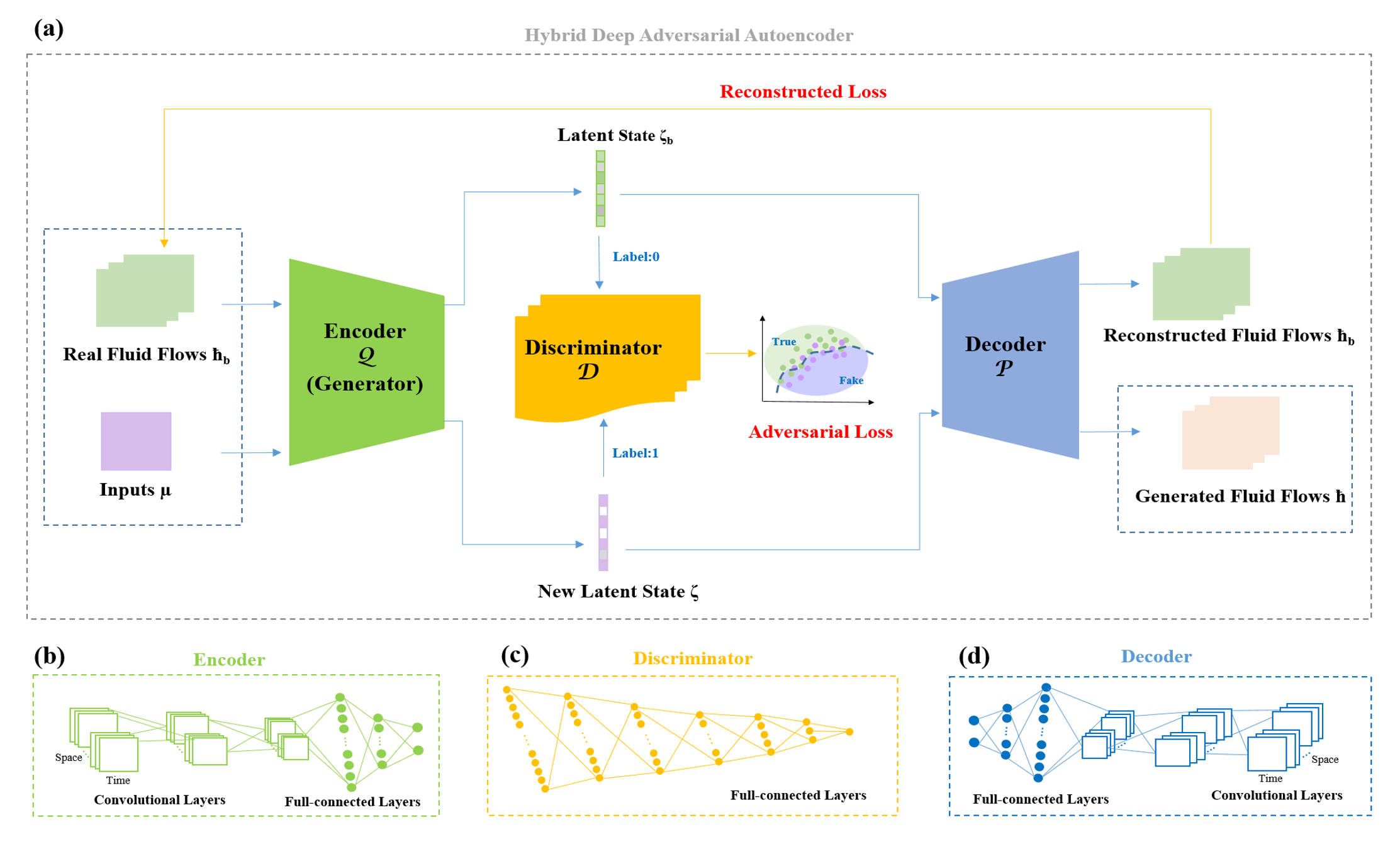
Given the parameter vector ${\mu=[{\mu^{1}},{\mu^{2}},...,{\mu^{{N_{x}}}}]}$ as inputs and the state variable vector ${\hbar_{b}=[{\hbar_{b}^{1}},{\hbar_{b}^{2}},...,{\hbar_{b}^{{N_{x}}}}]}$ as the targeted outputs, the model architectur of the hybrid DAA are shown in Fig. 1.

5 Numerical examples

The example used for validation of the hybrid DAA is a case of water column collapse. It is a benchmark test case for multi-material models, which is also known as a dam break problem. The dam-break flow problem has been of great importance in hydraulic engineering and hydropower generation. Dam-break flows are complex and generally discontinuous with abrupt variations of flow velocity and water depth (Seyedashraf et al., 2017). The flooding induced by the dam-break flows causes great loss of human life and property as well as damaging the ecosystem in the downstream area.

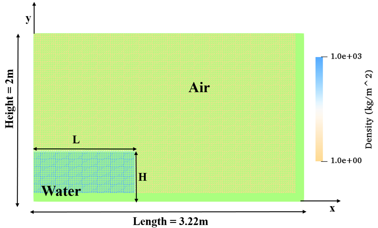
In this example, the dam-break experiment conducts in a tank with the length ${3.22m}$, the height ${2m}$, and the depth ${1m}$ (Zhou et al., 1999). The simulated reservoir of water is held behind a barrier at one end of the tank. For no variations are introduced in the third dimension, the experiment is reproduced in the horizontal and vertical dimensions within the domain area ${\Omega}$. Fig. 2 shows the mesh in the domain area ${\Omega}$. The dam break problem is simulated using the unstructured mesh finite element fluid model (${Fluidity}$) (Pain et al., 2001)(referred as the original high fidelity model). The densities of water and air are ${1,000kg{m^{-2}}}$ and ${1kg{m^{-2}}}$ respectively. The scalar fields ${a_{k}}$ representing the volume fraction is introduced to distinguish the two materials. As shown in Fig. 2, the interface between the water (the yellow area, ${a_{k}=1}$) and air (the blue area, ${a_{k}=0}$) is delineated by contours at ${a_{k}}$ of $0.025$, $0.5$ and $0.975$. In this case, the simulation period is ${[0,1.85]s}$, with a timestep = ${0.025s}$. Thus, the targeted fluid flows ${\hbar_{d}}$ were obtained by running the original high fidelity model, with a unstructured mesh of 19097 nodes.

Figure 2: The sketch of water collapse experiment.

5.1 Model appplication

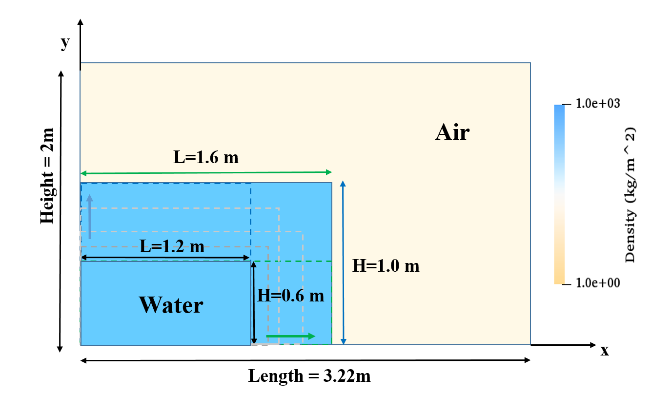
Data collection: In this case, for training the hybrid DAA, the length $L$ and height $H$ of the tank are selected as the input parameters (as shown in Fig. 3). The length of the tank $L$ is ranged from 1.2 $m$ to 1.6 $m$, and the height $H$ of the tank varies from 0.6 $m$ to 1.0 $m$. A series of sizes as inputs $\mu$ and the corresponding solution snapshots ${\hbar_{d}}$ (a total of 3375 snapshots of 45 pairs of input-output) were obtained by running the high fidelity model, which can be re-written in a time discretized form:

$$\mu=[{\mu^{1}_{a}},{\mu^{2}_{a}},...,{\mu^{{N_{x}}}_{a}}],{(a\in[0,44],{N_{x}}=19097)},$$ (15)

$$\hbar_{d}=\left[{\begin{array}[]{*{20}{c}}{\hbar_{d,a,{t_{1}}}^{1}}&{\hbar_{d,a,{t_{1}}}^{2}}&\cdots&{\hbar_{d,a,{t_{1}}}^{{N_{x}}}}\\ {\hbar_{d,a,{t_{2}}}^{1}}&{\hbar_{d,a,{t_{2}}}^{2}}&\cdots&{\hbar_{d,a,{t_{2}}}^{{N_{x}}}}\\ \vdots&\vdots&{}\hfil&\vdots\\ {\hbar_{{d,a,t_{{N_{t}}}}}^{1}}&{\hbar_{{d,a,t_{{N_{t}},}}}^{2}}&\cdots&{\hbar_{{d,a,t_{{N_{t}},}}}^{{N_{x}}}}\end{array}}\right],{(a\in[0,44],{N_{x}}=19097,{N_{t}}=75)}.$$ (16)

The training and validated input-output pairs ${\vartheta_{tr}}$ and ${\phi_{tr}}$ (where ${\mu_{a}\in{\mathbb{R}^{{}^{N_{x}}}}},{\hbar_{d,a}\in{\mathbb{R}^{{}^{N_{x}\times N_{t}}}}}$, $a\in[0,38],{N_{x}}=75,{N_{t}}=19097$) are selected for model training and parameter optimization, while the remained inputs ${(\vartheta\backslash{\vartheta_{tr}})}$ (where ${\mu_{a}\in{\mathbb{R}^{{}^{N_{x}}}},a\in[0,6],{N_{x}}=19097}$) are used for model prediction.

Figure 3: The setttings of length and height in water collapse experiment.

5.2 Model Prediction

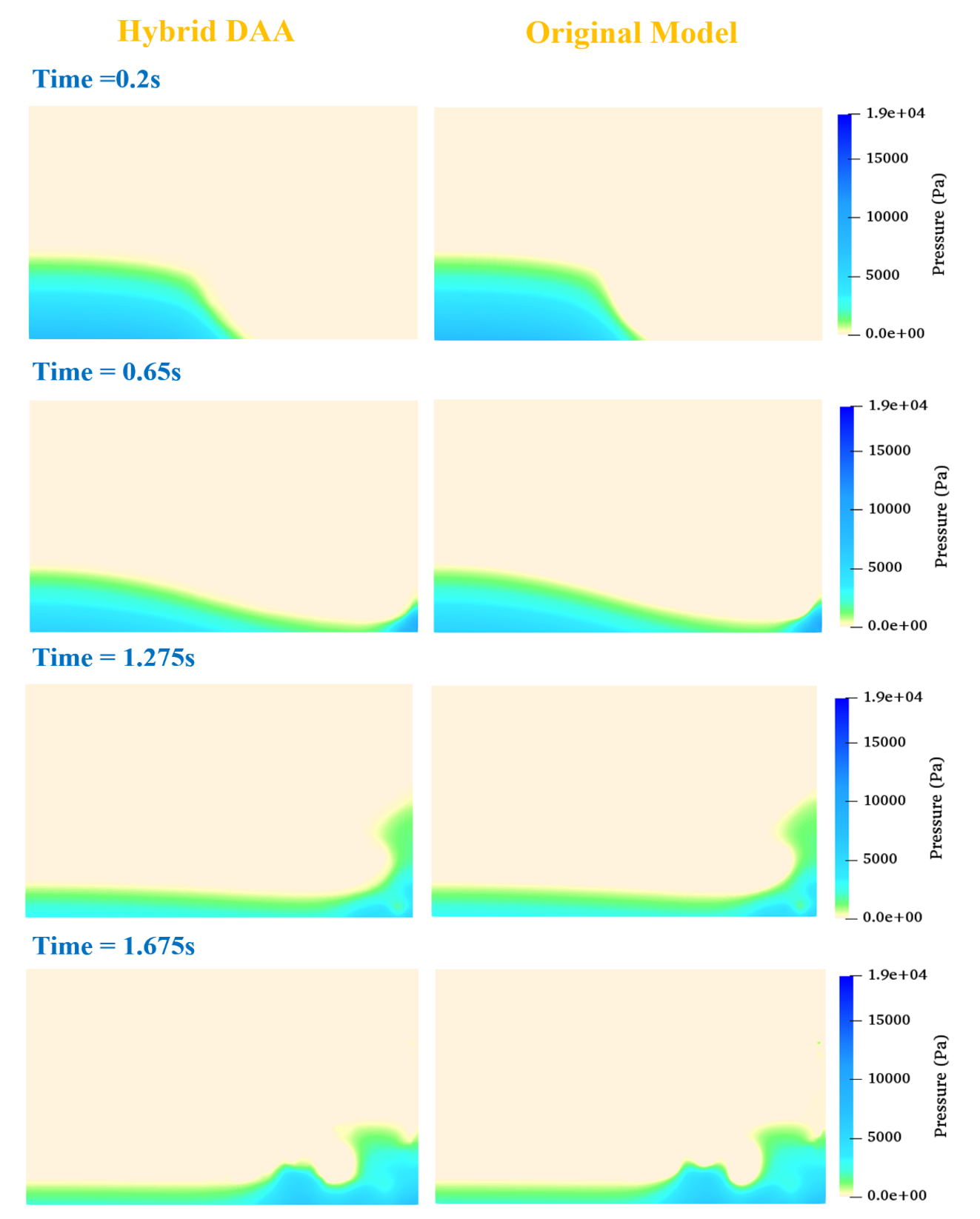
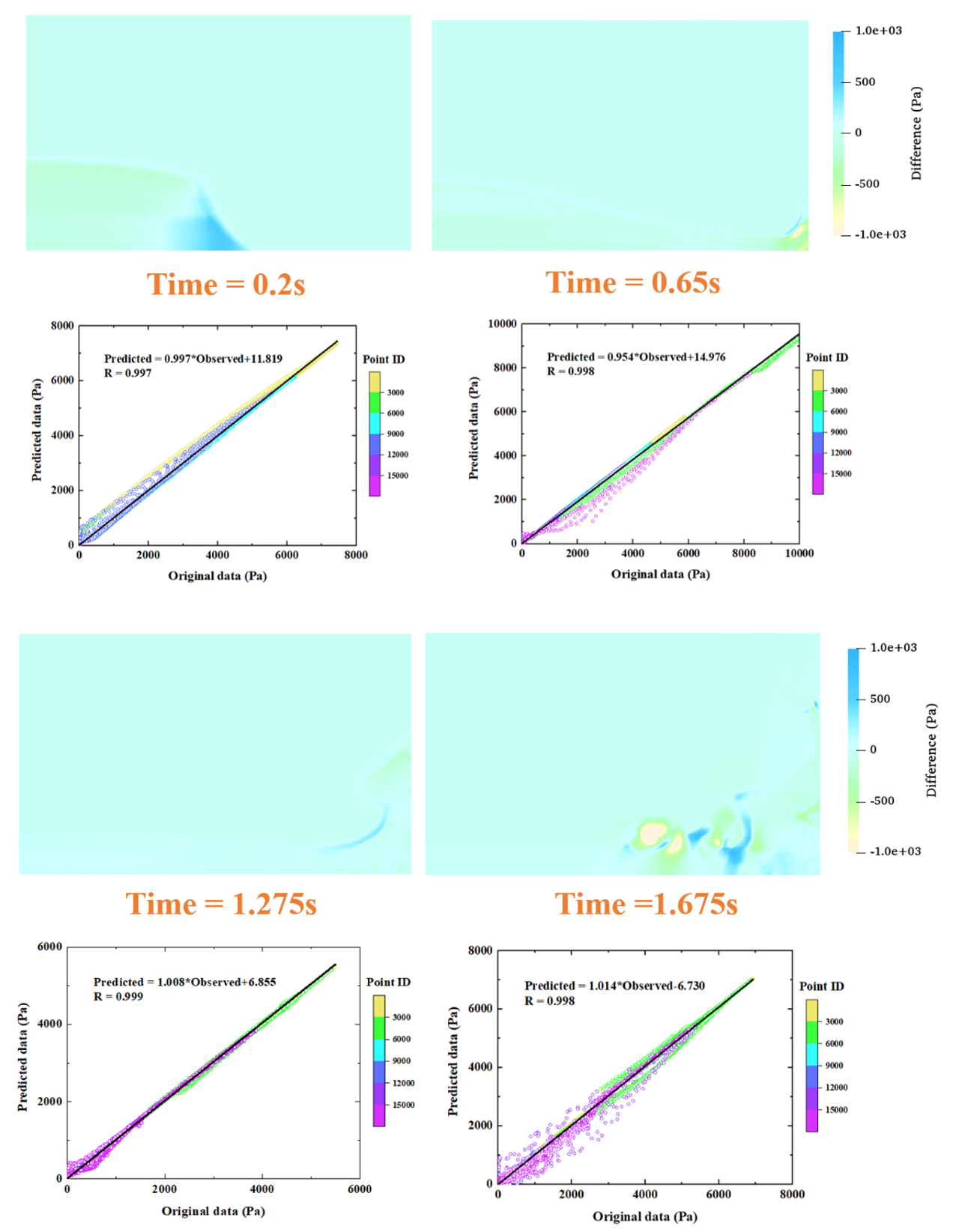
Prediction of spatial nonliear fluid flows: To evaluate the predictive ability of the hybrid DAA, given the new input ${\mu\in(\vartheta\backslash{\vartheta_{tr}})}$, comparison of the predictive results from the hybrid DAA and the original high fidelity model are shown in Fig. 4. It can be seen that the hybrid DAA predicted the flow fields well, which captures the most pressure features at time levels $t=0.2,0.65,1.275,1.675s$. Visually, very little difference between the hybrid DAA and the original high fidelity model can be noticed. In order to compare the differences between the predictive and original fluid fields, the absolute error and correlation coefficient of pressure solutions within the computational domain area $\Omega$ are illustrated in Fig. 5. It is observed that the absolute errors are small over the whole domain area at different time levels, and the correlation coefficient between the hybrid DAA and the high fidelity model is higher than $0.99$. The predictive results in spatial space suggest the hybrid DAA is able to obtain reasonable and accurate solutions in spatial space for nonlinear fluid flows.

Figure 4: Comparison of the spatial distribution of pressure fields obtained from the hybrid DAA (left) and the original high fidelity model (right) at time levels $t=0.2,0.65,1.275,1.675s$.

Figure 5: Differences and correlation coefficients of pressure fields between the hybrid DAA and the original high fidelity model at time levels $t=0.2,0.65,1.275,1.675s$.

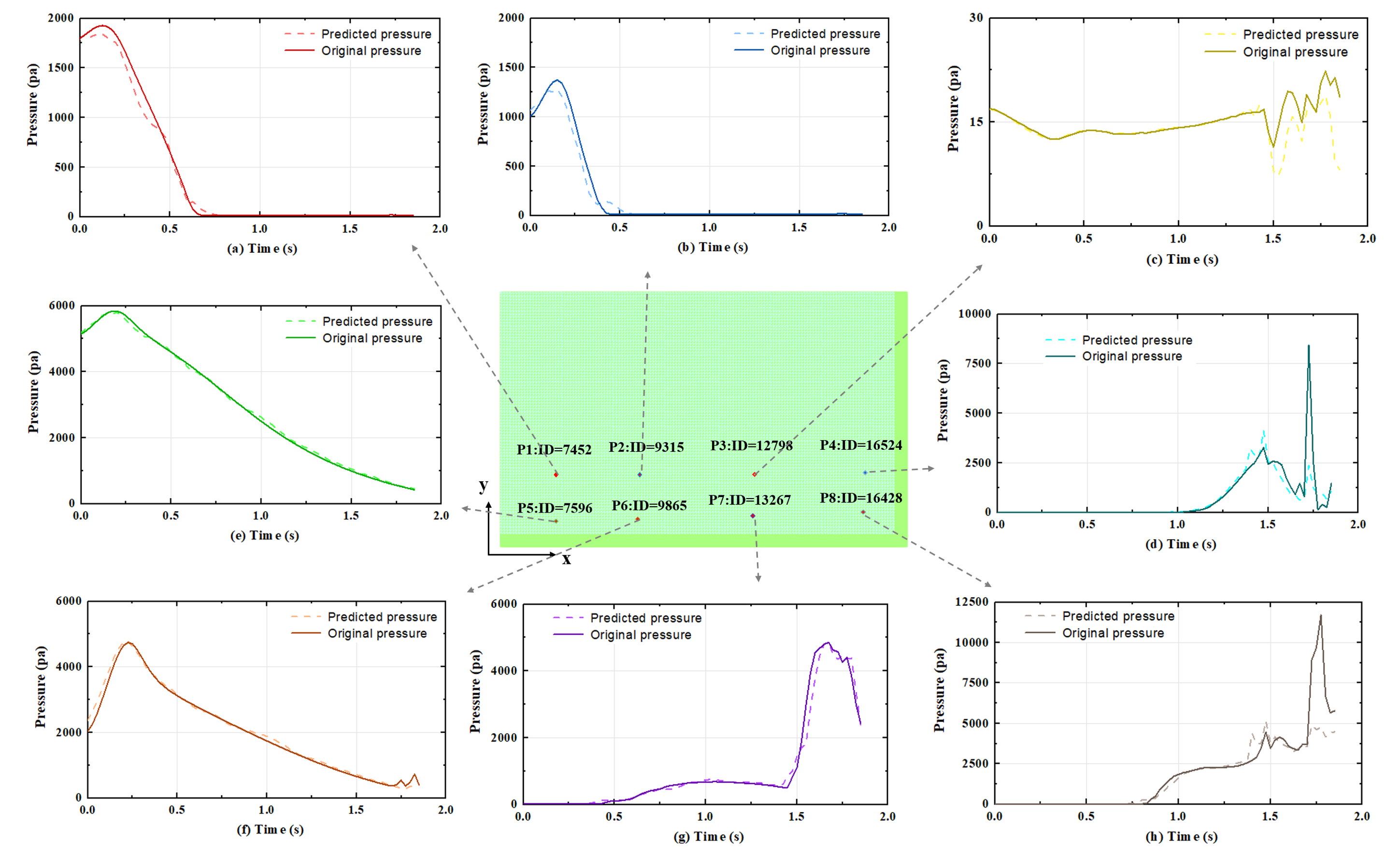
Prediction of temporal nonliear fluid flows: Fig. 6 shows the temporal variation of pressure solution predicted by the two models. Before the water collapse happens, the points P1, P2, P5 and P6 are located in the water area (as marked with a blue rectangle in Fig. 3), while other four points P3, P4, P7 and P8 are placed in the area filled with air. Model performance has been evaluated by comparison of pressure variation in these detector points. In the Fig. 6(a), (b), (e) and (f), the pressure values at four points are slightly increased and then gradually decreased as the water collapse happens. As for detector P3, it is beyond the scale of water front motions before $t=1.5s$, and the pressure trend in Fig. 6(c) is not so obvious. After $t=1.5s$, influenced by the overturning water, the pressure at the detector P3 starts to fluctuate. Compared to detector P3, it can be noted that the pressure values at detector P4, P7 and P8 are uprising when the water drops down the horizon into rightward direction. The sequent water experiences dropping, traveling, rising up along the right vertical wall, and dropping again processes. It can be observed that the curves of pressure from the hybrid DAA achieve a good agreement with that of the original high fidelity model, except for the under-predictions of dropping again process after $t=1.5s$. However, it is also a challenge problem for numerical simulation when the water hits at the right wall and again meets the horizontal free surface (Park et al., 2009).

Figure 6: Comparison of the temporal variation of pressure at points ID = 7452, 7596, 9315, 9865, 12798, 13267, 16428, 16524.

Model performance anaylsis: To further evaluate the performance of the hybrid DAA, the correlation coefficient and RMSE are calculated in temporal and spatial space, respectively. The error analysis of pressure solutions in temporal space is shown in Fig. 7. It is evident that the values of RMSE are between $0pa$ to $2000pa$ while the correlation coefficients are above ${90\%}$. In light of fluid field prediction in temporal space, these results demonstrate that the hybrid DAA performs well and the predicted fluid fields are in good agreement with the true fluid fields.

Figure 7: The correlation coefficients and RMSE of pressure between the generated fields and original high fidelity fields during whole simulational period.

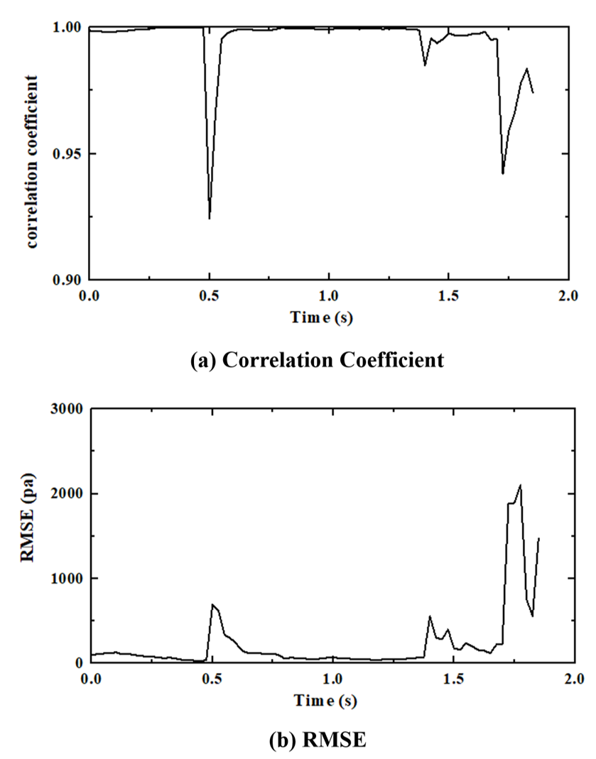
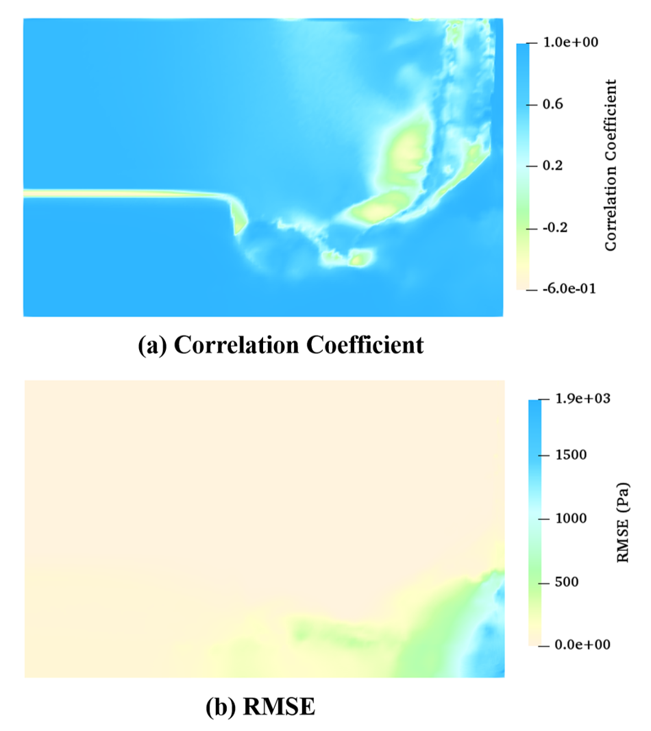
Fig. 8 illustrates the model performance in spatial space. It can be noted that the RMSE is not beyond $1900pa$ in the whole domain area $\Omega$, which demonstrates the capability of hybrid DAA to predict accurate fluid flows. However, the correlation coefficient is negative in some area, where is affected by the water jet. When the water front strike the right vertical wall, the water jet causes a sudden rise of pressure and air entrainment (Park et al., 2009). The phenomena is decribed in Fig. 6(c), where depicts the pressure fluctuation after $t=1.5s$. Except for the area influenced by the interface of multi-materials, the correlation coefficient is beyond $0.9$ in the domain area $\Omega$.

Figure 8: The correlation coefficients and RMSE of pressure in time series in the computational domain area $\Omega$.

5.3 Model efficiency

The simulations of the hybrid DAA and the original high fidelity model were preformed on Intel Xeon(R) CPU@ 3.60GHz with a 449.5 GB memory. The computation time required for the hybrid DAA in online prediction process is $21.76s$, while $8836.67s$ for running the original high fidelity model. It can be seen that the CPU time for running the hybrid DAA is reduced drastically by three orders of magnitude in comparison to the original high fidelity model.

6 Conclusions

In this work, a hybrid DAA method has been, for the first time, used to predict nonlinear fluid flows in varying parameterized space. For any given input parameters $\mu$, the hybrid DAA is capable of predicting accurate dynamic nonlinear fluid flows and remains high efficiency in simulation, which takes both advantages of VAE and GAN.

The performance of the hybrid DAA has been demonstrated by a water collapse test case. To evaluate the model accuracy, a detailed comparison between the original high fidelity model (Fluidity) and the hybrid DAA has been undertaken. The accuracy assessment has also been performed through the correlation coefficient and RMSE. The numerical simulations show that the hybrid DAA exhibits good agreement with the original high fidelity model, in both space and time. Additionally, a significant CPU speed-up has been achieved by the hybrid DAA.

The hybrid DAA is an efficient and robust tool for parameterized modelling and prediction of nonlinear fluid flows. It provides a wide range of applications, for instance, risk response management in emergencies and natural hazards (e.g. flooding, dam break, etc), real-time decision making. Future work will be focused on the predictive ability of lead-time by the hybrid DAA and more complex fluid problems can also be examined with this model.

References

- Brunton et al. (2019) Brunton SL, Noack B, Koumoutsakos P. Machine learning for fluid mechanics. ArXiv 2019;abs/1905.11075.
- Erichson et al. (2019) Erichson NB, Muehlebach M, Mahoney MW. Physics-informed autoencoders for lyapunov-stable fluid flow prediction. arXiv preprint arXiv:190510866 2019;.
- Fang et al. (2017) Fang F, Pain C, Navon IM, Xiao D. An efficient goal-based reduced order model approach for targeted adaptive observations. International Journal for Numerical Methods in Fluids 2017;83(3):263–75.
- Farimani et al. (2017) Farimani AB, Gomes J, Pande VS. Deep learning the physics of transport phenomena. arXiv preprint arXiv:170902432 2017;.
- Geneva and Zabaras (2019) Geneva N, Zabaras N. Quantifying model form uncertainty in reynolds-averaged turbulence models with bayesian deep neural networks. Journal of Computational Physics 2019;383:125–47.
- Goodfellow (2016) Goodfellow I. Nips 2016 tutorial: Generative adversarial networks. arXiv preprint arXiv:170100160 2016;.
- Goodfellow et al. (2014) Goodfellow I, Pouget-Abadie J, Mirza M, Xu B, Warde-Farley D, Ozair S, Courville A, Bengio Y. Generative adversarial nets. In: Advances in neural information processing systems. 2014. p. 2672–80.
- Hou et al. (2017) Hou X, Shen L, Sun K, Qiu G. Deep feature consistent variational autoencoder. In: 2017 IEEE Winter Conference on Applications of Computer Vision (WACV). IEEE; 2017. p. 1133–41.
- Hu et al. (2019) Hu R, Fang F, Pain C, Navon I. Rapid spatio-temporal flood prediction and uncertainty quantification using a deep learning method. Journal of Hydrology 2019;.
- Humphrey et al. (2016) Humphrey GB, Gibbs MS, Dandy GC, Maier HR. A hybrid approach to monthly streamflow forecasting: integrating hydrological model outputs into a bayesian artificial neural network. Journal of Hydrology 2016;540:623–40.
- Isola et al. (2017) Isola P, Zhu JY, Zhou T, Efros AA. Image-to-image translation with conditional adversarial networks. In: Proceedings of the IEEE conference on computer vision and pattern recognition. 2017. p. 1125–34.
- Kim et al. (2019) Kim B, Azevedo VC, Thuerey N, Kim T, Gross M, Solenthaler B. Deep fluids: A generative network for parameterized fluid simulations. In: Computer Graphics Forum. Wiley Online Library; volume 38; 2019. p. 59–70.
- Kingma and Ba (2014) Kingma DP, Ba J. Adam: A method for stochastic optimization. arXiv preprint arXiv:14126980 2014;.
- Kingma and Welling (2013) Kingma DP, Welling M. Auto-encoding variational bayes. arXiv preprint arXiv:13126114 2013;.
- Kutz (2017) Kutz JN. Deep learning in fluid dynamics. Journal of Fluid Mechanics 2017;814:1–4.
- Latif et al. (2017) Latif S, Rana R, Qadir J, Epps J. Variational autoencoders for learning latent representations of speech emotion: A preliminary study. arXiv preprint arXiv:171208708 2017;.
- Lee and Carlberg (2018) Lee K, Carlberg K. Model reduction of dynamical systems on nonlinear manifolds using deep convolutional autoencoders. arXiv preprint arXiv:181208373 2018;.
- Li and Wand (2016) Li C, Wand M. Precomputed real-time texture synthesis with markovian generative adversarial networks. In: European Conference on Computer Vision. Springer; 2016. p. 702–16.
- Ling et al. (2016) Ling J, Kurzawski A, Templeton J. Reynolds averaged turbulence modelling using deep neural networks with embedded invariance. Journal of Fluid Mechanics 2016;807:155–66.
- Liu et al. (2017) Liu F, Xu F, Yang S. A flood forecasting model based on deep learning algorithm via integrating stacked autoencoders with bp neural network. In: 2017 IEEE third International conference on multimedia big data (BigMM). IEEE; 2017. p. 58–61.
- Lusch et al. (2018) Lusch B, Kutz JN, Brunton SL. Deep learning for universal linear embeddings of nonlinear dynamics. Nature communications 2018;9(1):4950.
- Mescheder et al. (2017) Mescheder L, Nowozin S, Geiger A. Adversarial variational bayes: Unifying variational autoencoders and generative adversarial networks. In: Proceedings of the 34th International Conference on Machine Learning-Volume 70. JMLR. org; 2017. p. 2391–400.
- Mohan and Gaitonde (2018) Mohan AT, Gaitonde DV. A deep learning based approach to reduced order modeling for turbulent flow control using lstm neural networks. arXiv preprint arXiv:180409269 2018;.
- Murata et al. (2019) Murata T, Fukami K, Fukagata K. Nonlinear mode decomposition for fluid dynamics. arXiv preprint arXiv:190604029 2019;.
- Pain et al. (2001) Pain C, Umpleby A, De Oliveira C, Goddard A. Tetrahedral mesh optimisation and adaptivity for steady-state and transient finite element calculations. Computer Methods in Applied Mechanics and Engineering 2001;190(29-30):3771–96.
- Park et al. (2009) Park I, Kim K, Kim J, Van S. A volume-of-fluid method for incompressible free surface flows. International Journal for Numerical Methods in Fluids 2009;61(12):1331–62.
- Pu et al. (2016) Pu Y, Gan Z, Henao R, Yuan X, Li C, Stevens A, Carin L. Variational autoencoder for deep learning of images, labels and captions. In: Advances in neural information processing systems. 2016. p. 2352–60.
- Reed et al. (2016) Reed S, Akata Z, Yan X, Logeswaran L, Schiele B, Lee H. Generative adversarial text to image synthesis. arXiv preprint arXiv:160505396 2016;.
- Reichstein et al. (2019) Reichstein M, Camps-Valls G, Stevens B, Jung M, Denzler J, Carvalhais N, et al. Deep learning and process understanding for data-driven earth system science. Nature 2019;566(7743):195.
- Roberts et al. (2017) Roberts A, Engel J, Eck D. Hierarchical variational autoencoders for music. In: NIPS Workshop on Machine Learning for Creativity and Design. 2017. .
- Rosca et al. (2017) Rosca M, Lakshminarayanan B, Warde-Farley D, Mohamed S. Variational approaches for auto-encoding generative adversarial networks. arXiv preprint arXiv:170604987 2017;.
- Semeniuta et al. (2017) Semeniuta S, Severyn A, Barth E. A hybrid convolutional variational autoencoder for text generation. arXiv preprint arXiv:170202390 2017;.
- Seyedashraf et al. (2017) Seyedashraf O, Rezaei A, Akhtari AA. Dam break flow solution using artificial neural network. Ocean Engineering 2017;142:125–32.
- Simonovsky and Komodakis (2018) Simonovsky M, Komodakis N. Graphvae: Towards generation of small graphs using variational autoencoders. In: International Conference on Artificial Neural Networks. Springer; 2018. p. 412–22.
- Taira et al. (2019) Taira K, Hemati MS, Brunton SL, Sun Y, Duraisamy K, Bagheri S, Dawson S, Yeh CA. Modal analysis of fluid flows: Applications and outlook. arXiv preprint arXiv:190305750 2019;.
- Walker et al. (2016) Walker J, Doersch C, Gupta A, Hebert M. An uncertain future: Forecasting from static images using variational autoencoders. In: European Conference on Computer Vision. Springer; 2016. p. 835–51.
- Wu et al. (2016) Wu Y, Burda Y, Salakhutdinov R, Grosse R. On the quantitative analysis of decoder-based generative models. arXiv preprint arXiv:161104273 2016;.
- Xiao et al. (2019) Xiao D, Heaney C, Fang F, Mottet L, Hu R, Bistrian D, Aristodemou E, Navon I, Pain C. A domain decomposition non-intrusive reduced order model for turbulent flows. Computers & Fluids 2019;182:15–27.
- Xie et al. (2018) Xie Y, Franz E, Chu M, Thuerey N. tempogan: A temporally coherent, volumetric gan for super-resolution fluid flow. ACM Transactions on Graphics (TOG) 2018;37(4):95.
- Zhou et al. (1999) Zhou Z, De Kat J, Buchner B. A nonlinear 3d approach to simulate green water dynamics on deck. In: Proceedings of the Seventh International Conference on Numerical Ship Hydrodynamics, Nantes, France. 1999. p. 1–15.