A Multiple Power Law Distribution for Initial Mass Functions

Abstract

We introduce a new multi-power-law distribution for the Initial Mass Function (IMF) to explore its potential properties. It follows on prior work that introduced mechanisms accounting for mass accretion in star formation, developed within the framework of general evolution equations for the mass distribution of accreting and non-accreting (proto)stars. This paper uses the same fundamental framework to demonstrate that the interplay between a mass-dependent and a time-dependent step-like dropout rate from accretion leads to IMFs that exhibit multiple power laws for an exponential mass growth. While the mass-dependent accretion and its dropout is intrinsic to each star, the time-dependent dropout might be tied to a specific history such as the rapid consumption of nebular material by nearby stars or the sweeping away of some material by shock waves. The time-dependent dropout folded into the mass-dependent process of star formation is shown to have a significant influence on the IMFs.

1 Introduction

The distribution of stellar (and substellar) masses resulting from the star-formation – known as the initial mass function (IMF) – provides the initial conditions for subsequent main-sequence or brown-dwarf evolution. There are a variety of ideas for the mechanisms leading to the IMF. One idea rests on turbulence in molecular clouds which determines the core mass function (CMF). This then maps directly onto the IMF (Padoan & Nordlund, 2002, 2004; Hennebelle & Chabrier, 2008, 2009) in the sense that approximately a fixed proportion of the core mass goes into the star(s). The IMF has been treated very generally as a statistical outcome of multiple contributing phenomena, with random multiplicative processes yielding a lognormal distribution (Zinnecker, 1984). Another idea is that accretion processes set the intermediate and high mass power law tail of the IMF. Zinnecker (1982) showed that a Bondi accretion process would broaden an initial distribution of masses and lead to a power law tail that was similar to that observed for the IMF. Adams & Fatuzzo (1996) advanced the idea that the observed IMF is dominated more by the accretion termination processes than by the CMF. These latter two approaches put more emphasis on the temporal evolution of the actual star formation process.

Some of these ideas were combined in a hybrid model for the IMF, the modified lognormal power-law (MLP) model (Basu & Jones, 2004; Basu et al., 2015) that relied on the statistical picture for the initial seed masses and a deterministic exponential growth law for masses coupled with a probabilistic model for the termination times of the growth. The initial seed masses were taken to follow a lognormal distribution, but each object then accreted mass in a deterministic (exponential growth) fashion. The termination times of accretion were then chosen statistically from an exponential distribution. This is consistent with equally likely stopping probability of accretion in equal time intervals. However, Basu & Jones (2004) also pointed out that the exponential distribution of termination times was consistent with the deterministic model of an exponentially growing rate of seed production up until some final time $T$ when star-formation ends. In the MLP model, the limit $T\rightarrow\infty$ is employed, although this assumption can be relaxed. Furthermore, it is worth noting that the MLP distribution becomes a pure power-law distribution in the limit that the initial lognormal seed distribution has zero variance, i.e., is a delta function. The index of the power law in the differential number per logarithmic mass bin is $\alpha\equiv\delta/\gamma$, which is the dimensionless ratio of the termination rate $\delta$ of accretion and the growth rate $\gamma$ of mass in an individual object.

Myers (2011) developed a model for the IMF based on equally likely stopping and also a hybrid mass growth law that had an initially constant mass accretion rate that later transitioned (at a specific mass) into a rapidly increasing value that could be characterized as exponential growth, Bondi accretion, or some intermediate growth law. He found a peaked IMF even when starting with all protostars having zero mass at an initial time. This led to an IMF that resembled the field star IMFs of Kroupa (2002) and Chabrier (2005) for suitable values of the transition mass, the characteristic timescale of accretion termination, and parameters describing the rapid mass growth at late times.

Recently, Hoffmann et al. (2018) showed that it is possible to produce a peaked IMF with dual power law (DPL) behavior when all protostars start with very small initial masses, thereby also removing the need to start with an an initial lognormal distribution of seed masses to produce a peaked IMF. The derivation in the following sections is a direct sequel of that paper. We advise the reader to consult Hoffmann et al. (2018) in order to develop a deeper appreciation of the formalism. Hoffmann et al. (2018) developed the peaked IMF based on a special case of general evolution equations for the distribution function of protostars still accreting and that for stars that are no longer accreting. These evolution equations account for the rearrangement in time of the probability to find a (proto)star of a certain mass due to the accretion of mass or other specifiable processes that need not be purely deterministic or stochastic in nature. The evolution equations in play are sufficiently general that, for example, the MLP can be rediscovered through these means. The new feature in Hoffmann et al. (2018) is a dropout rate that is initially small but rises to its final value in a sigmoid fashion at a certain time (and therefore also mass) and with a characteristic temporal width $\eta^{-1}$. “Sigmoid" means that the function transits in an s-shaped form from its $-\infty$-limit to its $\infty$-limit. One can envision this transition as a smoothed or smeared out Heavyside step function. Accordingly, for greater masses there is an increased probability that a star will stop accretion. In that sense the accretion in stars is a self-limiting process. The result is a dual power law distribution (DPL). The DPL has a rising power law $\text{d}n/\text{d}\log M\propto M^{2\beta}$ at low mass with index $\beta=\eta/\gamma$, in which $\eta$ is the dropout rise rate, and a declining power law at intermediate and high mass $\text{d}n/\text{d}\log M\propto M^{-\alpha}$ with index $\alpha=\delta/\gamma$. The peak of the distribution is approximately at $m_{\rm S}$, the mass at which the transition to greater termination rate takes place. This transition may be physically associated with the onset of nuclear fusion within the protostar. This agrees with the generation of outflows at the onset of nuclear fusion, as suggested by Shu et al. (1987). Interestingly, such an IMF with two power laws has been suggested by observations of the ONC by Da Rio et al. (2012) and of the 25 Orionis group by Suárez et al. (2019).

The DPL model is a direct consequence of the increased dropout rate from stellar accretion beyond a certain mass. By its nature, it exhibits intrinsic properties of the star formation process and thus would induce universal properties of the type sought for the IMF. But accretion need not only be terminated due to intrinsic properties. Extrinsic growth limitation is also permissible in the evolution equation framework. This type of growth limitation has a distinct and different significance. While intrinsic limitation is associated with properties of a single star’s growth, extrinsic limitation may be associated with particular histories of the larger system.

Termination of accretion can be attributed to many possible events. These include dynamical ejection of protostars from small multiple systems, outflow driven clearing of surrounding gas, a finite available mass reservoir due to limits in core mass or a competition with neighboring accretors, and stellar feedback from massive stars in the same cluster associated with stellar winds, outflows, or ionization fronts (see review by Bonnell et al. (2007) and references therein for a discussion of these mechansims). These processes may follow a temporal order that is approximately the order written above. The ejections typically occur at the earliest times, outflows may require the onset of at least deuterium fusion, and the effect from nearby massive stars may be felt much later if at all. It is therefore reasonable to explore the idea of a further increase of the termination probability at a later time than the initial rise, which can be loosely called a “nebula time”. So for example, the initial rise of termination probability may reflect the transition from dynamical ejection driven termination to outflow driven termination, while the second rise may represent the transition from outflow driven termination to a mass starvation driven termination. The mass starvation could of course occur due to multiple causes as listed above. However, we resist the impulse to add even more steps of an increase in termination probability, focusing instead on the effect of a single notable change to the generative model for the DPL.

To illustrate the consequences of a second increase of the dropout rate, we return to the evolution equation machinery. This leads to a variation on the DPL model that introduces a second power law at intermediate to high masses, apart from the high mass power law decrease of the IMF. Interestingly, a three power law IMF is shown by Kroupa (2001, 2002). We follow the same methodology as in Hoffmann et al. (2018), employing an evolutionary approach that accounts for both accreting objects and those that have dropped out of the accretion process according to a specified dropout rate. This methodology is quite general and can be expanded to increasing levels of complexity in future work. It also emphasizes the time-dependent nature of the mass function within any star-forming region. Recent work by Drass et al. (2016) and Jerabkova et al. (2019) shows that the Orion Nebula Cluster has had several episodes of star formation evidenced by distinct stellar populations of different ages.

Section 2 of this paper presents the derivation of the new multi-power-law distribution, while Section 3 illustrates its various properties and limits. Section 4 shows a comparison with some published IMF estimates and our conclusions are stated in Section 5.

2 A Probabilistic Description of Star Formation

The IMF describes the probability to find a star of mass $M$ in a star cluster. Here its probability density function is denoted as $P_{\text{IMF}}$. It will prove convenient to work in terms of $m=M/M_{\odot}$ or a monotonic increasing function $\xi$ of mass $m$, (e.g. $\xi=\log_{10}m$ or $\xi=\ln m$) to be specified as needed. We will none the less refer to $\xi$ as “mass".

2.1 The Accretion-Dropout Rates

A core element in our development is the dropout rate, which determines that fraction of stars which stop accretion as a function of time and mass. That fraction then becomes part of the IMF. The overall dropout rate we choose must reflect the two different sources of accretion stopping discussed above: the intrinsic and the extrinsic ones. Here we will thus employ an accretion dropout rate of special additive structure, namely

$$k(\xi,t)=k_{\text{$\xi$}}(\xi)+k_{\text{t}}(t),$$ (1)

where the mass-related term $k_{\text{$\xi$}}(\xi)$ reflects the intrinsic accretion stopping processes while the time-related term $k_{\text{t}}(t)$ reflects the extrinsic accretion stopping processes. As these processes are envisioned as occurring independent from each other, the corresponding accretion dropout rates should simply add. Each of those are chosen as sigmoid functions in the same fashion as in our previous work:

$$k_{\text{t}}(t) =\kappa_{\text{t}}/2(1+\tanh[(t-t_{\text{St}})\lambda_{\text{t}}]),$$ (2)

$$k_{\text{$\xi$}}(\xi) =\kappa_{\text{$\xi$}}/2(1+\tanh[(\xi-\xi_{\text{S$\xi$}})\beta_{\text{$\xi$}}]).$$ (3)

Both $t$ and $\xi$ have domains $-\infty$ to $\infty$.

Here $t_{\text{St}}$ is the characteristic (switch) time when the time-dependent dropout processes are switched on and lead to a maximum dropout rate of $\kappa_{\text{t}}$, which is the asymptotic value of the sigmoid function. $\xi_{\text{S$\xi$}}$ is the characteristic (switch) mass where the mass-dependent dropout processes are switched on and result in a maximum dropout rate of $\kappa_{\text{$\xi$}}$, which is the corresponding value for the mass case. The time and mass span of the transition zones are characterized by $1/\lambda_{\text{t}}$ and $1/\beta_{\text{$\xi$}}$ respectively.

2.2 Model Structure

The basis for our IMF theory is the overall probability density $P_{\text{tot}}(\xi,t)$ to find a condensation of mass $\xi$ at time $t$ in a cluster. Its normalization obeys $\int P_{\text{tot}}(\xi,t)\text{d}\xi=1$, which is reflected in the notation $P_{\text{tot}}(\xi,t)\,\text{d}\xi$ if we see the necessity to uniquely describe the mass variable with respect to which $P_{\text{tot}}(\xi,t)$ is a probability density. $P_{\text{tot}}(\xi,t)$ is the sum of the two probabilities $P_{\text{a}}(\xi,t)$ and $P_{\text{s}}(\xi,t)$, where $P_{\text{a}}(\xi,t)$ is the probability to find a condensation of mass $\xi$ still actively accreting at time $t$, and $P_{\text{s}}(\xi,t)$ is the probability to find a condensation of mass $\xi$ that has stopped accreting (and has thus become a member of the IMF):

$$P_{\text{tot}}(\xi,t)=P_{\text{a}}(\xi,t)+P_{\text{s}}(\xi,t).$$ (4)

The time evolution of $P_{\text{a}}(\xi,t)$ is described by

$$\partial_{t}P_{\text{a}}(\xi,t)={\cal L}P_{\text{a}}(\xi,t)-k(\xi,t)P_{\text{a}}(\xi,t),$$ (5)

where ${\cal L}$ is an operator describing the changes in $P_{\text{a}}(\xi,t)$ due to the accretion process, and $k(\xi,t)P_{\text{a}}(\xi,t)$ describes the changes in $P_{\text{a}}(\xi,t)$ due to the dropout processes. Thus $k(\xi,t)P_{\text{a}}(\xi,t)$ is that part of $P_{\text{a}}(\xi,t)$, which becomes inactive, or stationary, per time unit and thus a member of the IMF. Note, that the evolution operator ${\cal L}$ might describe a deterministic accretion of mass, but it might also be a probabilistic operator like a Fokker-Planck operator.

The evolution equation (5) is supplemented with an initial condition $P_{\text{a}}(\xi,t_{0})=P_{\text{a,0}}(\xi)$ which we choose, as in our previous paper, to be

$$P_{\text{a,0}}(\xi)=\hat{\delta}(\xi-\xi_{0}),$$ (6)

where $\hat{\delta}$ represents the Dirac delta function, in contrast to the unrelated constant $\delta$ used in the introduction. This choice reflects that all condensations are assumed to start with the same mass $\xi_{0}$.

As $P_{\text{s}}(\xi,t)$ is the probability to find a condensation of mass $\xi$ which has stopped accreting, it can be calculated by the time integral of all deactivated parts of $P_{\text{a}}(\xi,t)$ and thus obeys

$$P_{\text{s}}(\xi,t)=\int_{t_{0}}^{t}k(\xi,t^{\prime})P_{\text{a}}(\xi,t^{\prime})\text{d}t^{\prime},$$ (7)

with $t_{0}$ being the time for the onset of star formation, which without loss of generality is set to zero. The IMF is then given by

$$P_{\text{IMF}}(\xi)=\lim_{t\to\infty}P_{\text{s}}(\xi,t)=\int_{0}^{\infty}k(\xi,t^{\prime})P_{\text{a}}(\xi,t^{\prime})\text{d}t^{\prime}.$$ (8)

The limit $t\to\infty$ is a simplification in the following sense: In the statistical description of distributions the Gaussian distribution, which has an infinite domain, is often used for a variable which has a finite domain. For instance, the height of people have a finite range, none the less the Gaussian is used for its description. This is effective, since there is very little probability in the tails of the distribution, but then – in order to keep the normalization correct – one has to extend the integration to infinity. While the star formation in a cluster is occurring over a finite time and with a finite mass span, we will for simplicity sometimes extend the time and mass regime to $-\infty$ to $\infty$.

2.3 Accretion Rate

Following the literature (Basu & Jones, 2004; Basu et al., 2015; Hoffmann et al., 2018) we now make a further simplifying assumption, namely that the mass accretion is proportional to the already accreted mass. In the literature several different accretion growth laws have been proposed, for example the Bondi rate has mass accretion proportional to mass squared. Here we will restrict ourselves to a deterministic evolution law with a mass accretion proportional to the already accreted mass

$$\frac{\text{d}\ln m}{\text{d}t}=\gamma.$$ (9)

Thus a condensation with initial mass $m_{0}$ at time $t_{0}=0$ is transported in time $t$ to $m=m_{0}e^{\gamma t}$. We now introduce the probability distribution $P_{\text{aa}}(\xi,t)$, which would evolve from the initial distribution $P_{\text{aa}}(\xi,0)=P_{\text{a,0}}(\xi)$ for a vanishing dropout rate, i.e. $k(\xi,t)=0$,

$$\partial_{t}P_{\text{aa}}(\xi,t)={\cal L}P_{\text{aa}}(\xi,t),$$ (10)

and which keeps its normalization as all condensations are always active. With the choice $\xi=\ln m$ the corresponding evolution operator is then ${\cal L}[\xi]=-\gamma\partial_{\xi}$ and we find

$$\partial_{t}P_{\text{aa}}(\xi,t)=-\gamma\partial_{\xi}P_{\text{aa}}(\xi,t).$$ (11)

This is simply the half wave equation, which then shifts the initial distribution of $P_{\text{aa}}(\xi,0)$ uniformly to greater masses,

$$P_{\text{aa}}(\xi,t) =P_{\text{aa,0}}(\xi-\gamma t)=\hat{\delta}(\xi-\xi_{0}-\gamma t),$$ (12)

where eq. (6) has been used.

2.4 Accretion Dropout Rate

Now, we cross over from a vanishing accretion dropout rate ($k(\xi,t)=0$) to a finite accretion dropout rate ($k(\xi,t)\neq 0$). Let us assume that the evolution operator only depends on $\xi$, ${\cal L}={\cal L}[\xi]$, and the accretion-dropout rate is the sum of two contributions, as given in eq. (1)

$$k(\xi,t)=k_{\text{$\xi$}}(\xi)+k_{\text{t}}(t),$$

Then (5) becomes

$$\partial_{t}P_{\text{a}}(\xi,t)={\cal L}[\xi]P_{\text{a}}(\xi,t)-(k_{\text{$\xi$}}(\xi)+k_{\text{t}}(t))P_{\text{a}}(\xi,t).$$ (13)

We then use

$$P_{\text{a}}(\xi,t)=g_{\text{$\xi$}}(\xi)g_{\text{t}}(t)P_{\text{aa}}(\xi,t),$$ (14)

as an ansatz to decompose eq. (13),

$$g_{\text{$\xi$}}(\xi) P_{\text{aa}}(\xi,t)\;\partial_{t}g_{\text{t}}(t)+g_{\text{$\xi$}}(\xi)g_{\text{t}}(t)\;\partial_{t}P_{\text{aa}}(\xi,t)$$

$$= g_{\text{t}}(t)(-\gamma\partial_{\xi}g_{\text{$\xi$}}(\xi)P_{\text{aa}}(\xi,t))$$

$$-(k_{\text{$\xi$}}(\xi)+k_{\text{t}}(t))g_{\text{$\xi$}}(\xi)g_{\text{t}}(t)P_{\text{aa}}(\xi,t)$$

$$= -\gamma g_{\text{t}}(t)g_{\text{$\xi$}}(\xi)\partial_{\xi}P_{\text{aa}}(\xi,t)-\gamma g_{\text{t}}(t)P_{\text{aa}}(\xi,t)\partial_{\xi}g_{\text{$\xi$}}(\xi)$$

$$-k_{\text{$\xi$}}(\xi)g_{\text{$\xi$}}(\xi)g_{\text{t}}(t)P_{\text{aa}}(\xi,t)-k_{\text{t}}(t)g_{\text{$\xi$}}(\xi)g_{\text{t}}(t)P_{\text{aa}}(\xi,t).$$ (15)

Dividing eq. (15) by our product ansatz for $P_{\text{a}}(\xi,t)$ we get

$$\frac{\partial_{t}g_{\text{t}}(t)}{g_{\text{t}}(t)}+k_{\text{t}}(t)+\frac{\gamma\;\partial_{\xi}g_{\text{$\xi$}}(\xi)}{g_{\text{$\xi$}}(\xi)}+k_{\text{$\xi$}}(\xi)$$

$$+\frac{\partial_{t}P_{\text{aa}}(\xi,t)}{P_{\text{aa}}(\xi,t)}+\frac{\gamma\;\partial_{\xi}P_{\text{aa}}(\xi,t)}{P_{\text{aa}}(\xi,t)}=0$$ (16)

Using eq. (11) we see that the last two terms in the above equation cancel and we are left with

$$\left(\frac{\partial_{t}g_{\text{t}}(t)}{g_{\text{t}}(t)}+k_{\text{t}}(t)\right)+\left(\frac{\gamma\;\partial_{\xi}g_{\text{$\xi$}}(\xi)}{g_{\text{$\xi$}}(\xi)}+k_{\text{$\xi$}}(\xi)\right)=0.$$ (17)

Generalizing the approach we have taken in our previous paper (Hoffmann et al., 2018), we split the above equation into two parts to obtain separate evolution equations for the $g_{\text{t}}(t)$ and $g_{\text{$\xi$}}(\xi)$:

$$\partial_{t}g_{\text{t}}(t)=-k_{\text{t}}(t)g_{\text{t}}(t),$$ (18)

and

$$\gamma\partial_{\xi}g_{\text{$\xi$}}(\xi)=-k_{\text{$\xi$}}(\xi)g_{\text{$\xi$}}(\xi),$$ (19)

which are supplemented with the initial conditions $g_{\text{t}}(t)=1$ at $t=0$ and $g_{\text{$\xi$}}(\xi)=1$ at $\xi=\xi_{0}$. In this way $g_{\text{$\xi$}}(\xi)$ and $g_{\text{t}}(t)$ capture the decrease of probability in $P_{\text{a}}(\xi,t)$ due to the mass-related and the time-related dropout processes, respectively. Due to the additive structure of the dropout rate, each $g$ can do that separately from the other.

Inserting $P_{\text{aa}}(\xi,t)$ from eq. (12) into the ansatz eq. (14), and that into eq. (8) then gives us the IMF for $\xi\geq\xi_{0}$ as

$$P_{\text{IMF}}(\xi)=\int_{0}^{\infty}(k_{\text{t}}(t^{\prime})+k_{\text{$\xi$}}(\xi))\,g_{\text{t}}(t^{\prime})\,g_{\text{$\xi$}}(\xi)\,\hat{\delta}(\xi-\xi_{0}-\gamma t^{\prime})\,\text{d}t^{\prime}.$$ (20)

Table 1: Notation and meaning of all parameters.

Symbol	Meaning
$\kappa_{\text{t}}$	asymptotic maximum time-related dropout rate
$\kappa_{\text{$\xi$}}$	asymptotic maximum mass-related dropout rate
$t_{\text{St}}$	time-related Switch time,
	when time-related dropout becomes large
$\xi_{\text{S$\xi$}}$	(logarithm of) mass-related Switch mass,
	when mass-related dropout becomes large
$1/\lambda_{\text{t}}$	time span of the transition zone,
	during which time-related dropout becomes large
$1/\beta_{\text{$\xi$}}$	mass span of the transition zone
	during which mass-related dropout becomes large
$m_{0},\xi_{0}$	initial mass, (logarithm of initial mass)
$t_{0}$	initial time, onset of mass accretion, chosen to be 0
$\gamma$	accretion rate
$t_{\text{m}}$	needed accretion time to grow $m_{0}$ to $m$
$m_{\text{St}}$	time-related Switch mass,
	when time-related dropout becomes large
$m_{\text{S$\xi$}}$	mass-related Switch mass,
	when mass-related dropout becomes large
$\alpha_{\text{t}}$	dimensionless parameter, maximum time-related
	dropout rate in terms of the accretion rate
$\alpha_{\text{$\xi$}}$	dimensionless parameter, maximum mass-related
	dropout rate in terms of the accretion rate
$\beta_{\text{t}}$	dimensionless parameter, time span of the
	transition zone in terms of the inv. accretion rate
$P_{\text{a}}$	probability distribution of condensations (stars)
	which actively accrete
$P_{\text{s}}$	probability distribution of condensations (stars)
	which stopped accreting
$P_{\text{aa}}$	probability distribution of condensations (stars)
	which all always accrete due to missing dropout

2.5 The Truncated Multi Power Law IMF

Now the IMF, as given by the above equation, can be evaluated in closed form making use of the delta function features:

$$P_{\text{IMF}} (\xi)\;\text{d}(\xi)$$

$$=\int_{0}^{\infty}(k_{\text{t}}(t^{\prime})+k_{\text{$\xi$}}(\xi))\,g_{\text{t}}(t^{\prime})\,g_{\text{$\xi$}}(\xi)\,$$ (21)

$$\hskip 51.6665pt\times\hat{\delta}(\xi-\xi_{0}-\gamma t^{\prime})\,\text{d}t^{\prime}\;\text{d}(\xi)$$

$$=\int_{0}^{\infty}(k_{\text{t}}(t^{\prime\prime}/\gamma)+k_{\text{$\xi$}}(\xi))\,g_{\text{t}}(t^{\prime\prime}/\gamma)\,g_{\text{$\xi$}}(\xi)\,$$

$$\hskip 51.6665pt\times\hat{\delta}(\xi-\xi_{0}-t^{\prime\prime})\,\text{d}t^{\prime\prime}/\gamma\;\text{d}(\xi)$$

$$=(k_{\text{t}}((\xi-\xi_{0})/\gamma)+k_{\text{$\xi$}}(\xi))\,g_{\text{t}}((\xi-\xi_{0})/\gamma)\,$$

$$\hskip 51.6665pt\times g_{\text{$\xi$}}(\xi)/\gamma\;\text{d}(\xi)$$

$$=\begin{cases}0&:\;\xi<\xi_{0}\\ \frac{(k_{\text{t}}(t_{\text{m}})+k_{\text{$\xi$}}(\xi))\,g_{\text{t}}(t_{\text{m}})\,g_{\text{$\xi$}}(\xi)}{\gamma}\;\;\;\text{d}(\xi)&:\;\xi\geq\xi_{0},\end{cases}$$ (22)

where $t_{\text{m}}=(\xi-\xi_{0})/{\gamma}$. Inserting eq. (2) into eq. (18) and eq. (3) into eq. (19), while using the above initial conditions, we obtain the solutions

$$g_{\text{t}}(t) =e^{-\frac{\kappa_{\text{t}}}{2}t}\cosh[(t-t_{\text{St}})\lambda_{\text{t}}]^{-\frac{\kappa_{\text{t}}}{2\lambda_{\text{t}}}}\cosh[-t_{\text{St}}\lambda_{\text{t}}]^{\frac{\kappa_{\text{t}}}{2\lambda_{\text{t}}}},$$ (23)

$$g_{\text{$\xi$}}(\xi) =e^{-\frac{\kappa_{\text{$\xi$}}}{2\gamma}(\xi-\xi_{0})}\cosh[(\xi-\xi_{\text{S$\xi$}})\beta_{\text{$\xi$}}]^{-\frac{\kappa_{\text{$\xi$}}}{2\gamma\beta_{\text{$\xi$}}}}$$

$$\hskip 51.6665pt\times\cosh[(\xi_{0}-\xi_{\text{S$\xi$}})\beta_{\text{$\xi$}}]^{\frac{\kappa_{\text{$\xi$}}}{2\gamma\beta_{\text{$\xi$}}}}.$$ (24)

We now introduce the time-related dropout switch mass $m_{\text{St}}$ via $t_{\text{St}}=(\ln m_{\text{St}}-\ln m_{0})/{\gamma}$ and define dimensionless parameters $\alpha_{\text{t}}=\frac{\kappa_{\text{t}}}{\gamma}$ and $\beta_{\text{t}}=\frac{\lambda_{\text{t}}}{\gamma}$. Then by substituting $t_{\text{m}}$ and $t_{\text{St}}$ we find

$$\hat{g}_{\text{t}} (m,m_{0})=$$

$$e^{-\frac{\alpha_{\text{t}}}{2}\ln\frac{m}{m_{0}}}\cosh\left[\beta_{\text{t}}\ln\frac{m}{m_{\text{St}}}\right]^{-\frac{\alpha_{\text{t}}}{2\beta_{\text{t}}}}\cosh\left[\beta_{\text{t}}\ln\frac{m_{0}}{m_{\text{St}}}\right]^{\frac{\alpha_{\text{t}}}{2\beta_{\text{t}}}}.$$ (25)

Similarly we introduce the dimensionless parameter $\alpha_{\text{$\xi$}}=\frac{\kappa_{\text{$\xi$}}}{\gamma}$ to obtain

$$\hat{g}_{\text{$\xi$}} (m,m_{0})=$$

$$e^{-\frac{\alpha_{\text{$\xi$}}}{2}\ln\frac{m}{m_{0}}}\cosh\left[\beta_{\text{$\xi$}}\ln\frac{m}{m_{\text{S$\xi$}}}\right]^{-\frac{\alpha_{\text{$\xi$}}}{2\beta_{\text{$\xi$}}}}\cosh\left[\beta_{\text{$\xi$}}\ln\frac{m_{0}}{m_{\text{S$\xi$}}}\right]^{\frac{\alpha_{\text{$\xi$}}}{2\beta_{\text{$\xi$}}}}.$$ (26)

In addition we rewrite the dropout rates as

$$\hat{k}_{\text{t}}(m) =\frac{\alpha_{\text{t}}}{2}\left(1+\tanh\left[\beta_{\text{t}}\ln\frac{m}{m_{\text{St}}}\right]\right),$$ (27)

$$\hat{k}_{\text{$\xi$}}(m) =\frac{\alpha_{\text{$\xi$}}}{2}\left(1+\tanh\left[\beta_{\text{$\xi$}}\ln\frac{m}{m_{\text{S$\xi$}}}\right]\right).$$ (28)

To give a visualization of the dropout rates we plotted both, $\hat{k}_{\text{t}}(m)$ and $\hat{k}_{\text{$\xi$}}(m)$, in figure 1 for the parameter set $\alpha_{\text{t}}=6$, $\beta_{\text{t}}=3$, $m_{\text{St}}=10^{0}$, $\alpha_{\text{$\xi$}}=3$, $\beta_{\text{$\xi$}}=1$, and $m_{\text{S$\xi$}}=10^{-1}$ also used later.

Figure 1: The dropout rates $\hat{k}_{\text{t}}(m)$ and $\hat{k}_{\text{$\xi$}}(m)$ given in eq. (27) and (28) and their sum are given for the parameter set $\alpha_{\text{t}}=6$, $\beta_{\text{t}}=3$, $m_{\text{St}}=10^{0}$, $\alpha_{\text{$\xi$}}=3$, $\beta_{\text{$\xi$}}=1$, and $m_{\text{S$\xi$}}=10^{-1}$. We observe three regions: A low masses, B intermediate masses, and C high masses.

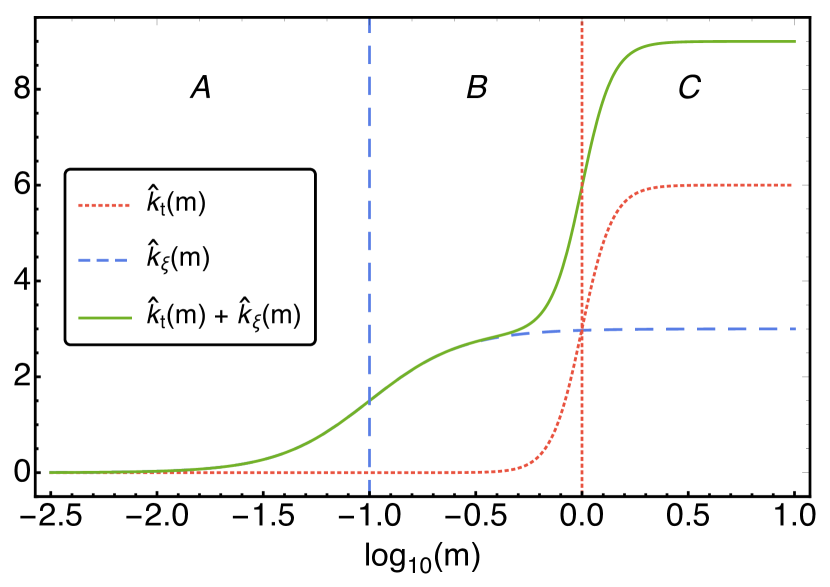
Combining these results we find for $m\geq m_{0}$ the truncated multi power law distribution $P_{\text{tMPL}}$ as

$$P_{\text{tMPL}} (m;\alpha_{\text{t}},\beta_{\text{t}},m_{\text{St}},\alpha_{\text{$\xi$}},\beta_{\text{$\xi$}},m_{\text{S$\xi$}},m_{0})\;\text{d}(\ln m)$$

$$=(\hat{k}_{\text{t}}(m)+\hat{k}_{\text{$\xi$}}(m))\hat{g}_{\text{t}}(m,m_{0})\hat{g}_{\text{$\xi$}}(m,m_{0})\,\text{d}(\ln m).$$ (29)

We named this distribution the truncated multi power law distribution as it is defined only for $m\geq m_{0}$, contrary to the multi power law distribution which will be defined below for all $m$. The truncated multi power law distribution $P_{\text{tMPL}}$ depends on seven dimensionless parameters. $\alpha_{\text{t}}=\frac{\kappa_{\text{t}}}{\gamma}$ and $\alpha_{\text{$\xi$}}=\frac{\kappa_{\text{$\xi$}}}{\gamma}$ measure the maximum dropout rates in terms of the mass growth rate, which provides the characteristic time unit. $\beta_{\text{t}}=\frac{\lambda_{\text{t}}}{\gamma}$ and $\beta_{\text{$\xi$}}$ give the mass span of the transition zones of the time- and mass-related dropout rates in terms of $\ln m$. Likewise $m_{\text{St}}$ and $m_{\text{S$\xi$}}$ define the switch masses for the onset of the increased dropout, and finally $m_{0}$ the initial mass at the accretion onset.

3 The Multi Power Law IMF

In order to simplify the IMF further we note that we can take the limit $m_{0}\to 0$ and obtain as a limiting distribution the Multi Power Law (MPL) IMF defined for all $m>0$:

$$P_{\text{MPL}} (m;\alpha_{\text{t}},\beta_{\text{t}},m_{\text{St}},\alpha_{\text{$\xi$}},\beta_{\text{$\xi$}},m_{\text{S$\xi$}})\;\text{d}m$$

$$=(\hat{k}_{\text{t}}(m)+\hat{k}_{\text{$\xi$}}(m))\;\hat{g}_{\text{t}}(m)\;\hat{g}_{\text{$\xi$}}(m)/m\,\text{d}m$$ (30)

$$=\hat{k}_{\text{t}}(m)\;\hat{g}_{\text{t}}(m)\;\hat{g}_{\text{$\xi$}}(m)/m\,\text{d}m+\hat{k}_{\text{$\xi$}}(m)\;\hat{g}_{\text{t}}(m)\;\hat{g}_{\text{$\xi$}}(m)/m\,\text{d}m$$

$$=P_{\text{MPL,t}}+P_{\text{MPL,$\xi$}},$$

with

$$\hat{g}_{\text{t}}(m) =2^{-\frac{\alpha_{\text{t}}}{2\beta_{\text{t}}}}e^{-\frac{\alpha_{\text{t}}}{2}\ln\frac{m}{m_{\text{St}}}}\cosh\left[\beta_{\text{t}}\ln\frac{m}{m_{\text{St}}}\right]^{-\frac{\alpha_{\text{t}}}{2\beta_{\text{t}}}}\;,$$ (31)

$$\hat{g}_{\text{$\xi$}}(m) =2^{-\frac{\alpha_{\text{$\xi$}}}{2\beta_{\text{$\xi$}}}}e^{-\frac{\alpha_{\text{$\xi$}}}{2}\ln\frac{m}{m_{\text{S$\xi$}}}}\cosh\left[\beta_{\text{$\xi$}}\ln\frac{m}{m_{\text{S$\xi$}}}\right]^{-\frac{\alpha_{\text{$\xi$}}}{2\beta_{\text{$\xi$}}}}\;,$$ (32)

and $\hat{k}_{\text{t}}(m)$ and $\hat{k}_{\text{$\xi$}}(m)$ from eq. (27) and eq. (28), respectively.

The transition from eq. (25) and eq. (26) to eq. (31) and eq. (32) is facilitated by using the small $x$ behavior of $\cosh[ax]=(e^{-ax}+e^{ax})/2$. For $ax\ll 0$ the first exponential dominates and we find $\cosh[ax]\approx e^{-ax}/2$. Applying this on the $m_{0}-\cosh$-term in eq. (25) for $a=\beta_{\text{t}}>0$ and $m_{0}\ll m_{\text{St}}$ and thus $x=\ln\frac{m_{0}}{m_{\text{St}}}\ll 0$ one gets

$$\hat{g}_{\text{t}} (m,m_{0})$$

$$\approx e^{-\frac{\alpha_{\text{t}}}{2}\ln\frac{m}{m_{0}}}\cosh\left[\beta_{\text{t}}\ln\frac{m}{m_{\text{St}}}\right]^{-\frac{\alpha_{\text{t}}}{2\beta_{\text{t}}}}2^{-\frac{\alpha_{\text{t}}}{2\beta_{\text{t}}}}\left(e^{-\beta_{\text{t}}\ln\frac{m_{0}}{m_{\text{St}}}}\right)^{\frac{\alpha_{\text{t}}}{2\beta_{\text{t}}}}$$

$$=e^{-\frac{\alpha_{\text{t}}}{2}\ln\frac{m}{m_{0}}}\cosh\left[\beta_{\text{t}}\ln\frac{m}{m_{\text{St}}}\right]^{-\frac{\alpha_{\text{t}}}{2\beta_{\text{t}}}}2^{-\frac{\alpha_{\text{t}}}{2\beta_{\text{t}}}}e^{-\frac{\alpha_{\text{t}}}{2}\ln\frac{m_{0}}{m_{\text{St}}}}$$

$$=2^{-\frac{\alpha_{\text{t}}}{2\beta_{\text{t}}}}e^{-\frac{\alpha_{\text{t}}}{2}\ln\frac{m}{m_{\text{St}}}}\cosh\left[\beta_{\text{t}}\ln\frac{m}{m_{\text{St}}}\right]^{-\frac{\alpha_{\text{t}}}{2\beta_{\text{t}}}},$$ (33)

which shows, that the leading term of this approximation is no longer $m_{0}$-dependent.

Applying in addition the above reasoning to the remaining $\cosh$-term in $\hat{g}_{\text{t}}(m)$ for $a=\beta_{\text{t}}>0$ and $m\gg m_{\text{St}}$ and thus $x=\ln\frac{m}{m_{\text{St}}}\gg 0$ leads to the large $m$ behavior of

$$\hat{g}_{\text{t}} (m)$$

$$\approx 2^{-\frac{\alpha_{\text{t}}}{2\beta_{\text{t}}}}e^{-\frac{\alpha_{\text{t}}}{2}\ln\frac{m}{m_{\text{St}}}}2^{\frac{\alpha_{\text{t}}}{2\beta_{\text{t}}}}\left(e^{\beta_{\text{t}}\ln\frac{m}{m_{\text{St}}}}\right)^{-\frac{\alpha_{\text{t}}}{2\beta_{\text{t}}}}$$

$$=\left(\frac{m}{m_{\text{St}}}\right)^{-\frac{\alpha_{\text{t}}}{2}}e^{-\frac{\alpha_{\text{t}}}{2}\ln\frac{m}{m_{\text{St}}}}=\left(\frac{m}{m_{\text{St}}}\right)^{-\alpha_{\text{t}}},$$ (34)

showing a power law decay for $\hat{g}_{\text{t}}(m)$. Similarly, $\hat{g}_{\text{$\xi$}}(m,m_{0})$ can then be handled and leads to $\hat{g}_{\text{$\xi$}}(m)$, which also shows a power law.

There are a number of interesting features of the MPL, some of which we will discuss in the following. Note that from a technical perspective the functional form of the time-dependent dropout rate and the mass-dependent dropout rate are equivalent.

The parameter set used as a standard set in the subsequent discussion is $\alpha_{\text{t}}=6$, $\beta_{\text{t}}=3$, $m_{\text{St}}=10^{0}$, $\alpha_{\text{$\xi$}}=3$, $\beta_{\text{$\xi$}}=1$, and $m_{\text{S$\xi$}}=10^{-1}$. These parameters are chosen exclusively for demonstrating the effects on the resulting IMF and not for a direct astrophysical application.

Figure 2: The MPL distribution given in eq. (30) is shown for two cases: one in which the mass dropout rate $\hat{k}_{\xi}$ is set to 0 ($\alpha_{\text{$\xi$}}=0$) but the time dropout rate $\hat{k}_{\text{t}}$ is nonzero ($\alpha_{\text{t}}=6$, $\beta_{\text{t}}=3$, and $m_{\text{St}}=10^{0}$), and one in which the time dropout rate $\hat{k}_{\text{t}}$ is set to 0 ($\alpha_{\text{t}}=0$) but the mass dropout rate $\hat{k}_{\xi}$ is nonzero ($\alpha_{\text{$\xi$}}=3$, $\beta_{\text{$\xi$}}=1$, and $m_{\text{S$\xi$}}=10^{-1}$). Here the low and the high mass end of the MPL distribution with $\hat{k}_{\xi}(m)=0$ has a steeper increase and decrease, respectively, than for the MPL distribution with $\hat{k}_{\text{t}}(m)=0$.

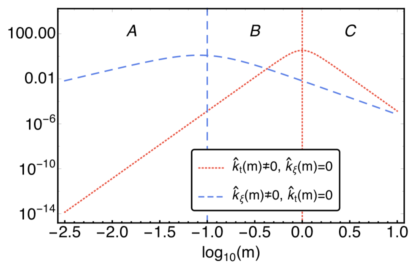
In figure 2 we show the $P_{\text{MPL}}(m;\alpha_{\text{t}},\beta_{\text{t}},m_{\text{St}},\alpha_{\text{$\xi$}},\beta_{\text{$\xi$}},m_{\text{S$\xi$}})$ for two variations of the standard set: one for which the mass dropout rate $\hat{k}_{\xi}$ is set to 0 ($\alpha_{\text{$\xi$}}=0$) but the time dropout rate $\hat{k}_{\text{t}}$ is nonzero ($\alpha_{\text{t}}=6$, $\beta_{\text{t}}=3$, and $m_{\text{St}}=10^{0}$), the other for which the time dropout rate $\hat{k}_{\text{t}}$ is set to 0 ($\alpha_{\text{t}}=0$) but the mass dropout rate $\hat{k}_{\xi}$ is nonzero ($\alpha_{\text{$\xi$}}=3$, $\beta_{\text{$\xi$}}=1$, and $m_{\text{S$\xi$}}=10^{-1}$). In both cases one finds the familiar form of the DPL distribution. We can immediately recognize three regions A, B, and C: region A where both MPLs increase, region B where the MPL with $\hat{k}_{\text{t}}=0$ decays while the one with $\hat{k}_{\text{$\xi$}}=0$ still increases, and region C where both decay. In each region there is a clear power law behaviour appearing in this log-log plot as straight lines.

We notice that the decay of the MPLs for high masses is due to the decay of $\hat{g}_{\text{t}}(m)$ and of $\hat{g}_{\text{$\xi$}}(m)$. These functions decay with a power law. Their respective exponents are $-\alpha_{\text{t}}$ and $-\alpha_{\text{$\xi$}}$. The dropout rates $\hat{k}_{\text{t}}(m)$ and $\hat{k}_{\text{$\xi$}}(m)$ on the other hand increase with power laws with exponents $2\beta_{\text{t}}$ and $2\beta_{\text{$\xi$}}$, respectively. The symmetry of the MPL with a mass dropout rate $\hat{k}_{\xi}=0$ makes it easy to recognize this: $\alpha_{\text{t}}=6=2\beta_{\text{t}}$.

Figure 3: $P_{\text{MPL}}$ and the corresponding time term $P_{\text{MPL,t}}$ and mass term $P_{\text{MPL,$\xi$}}$, as given in eq. (30), are shown for the standard parameter set ($\alpha_{\text{t}}=6$, $\beta_{\text{t}}=3$, $m_{\text{St}}=10^{0}$, $\alpha_{\text{$\xi$}}=3$, $\beta_{\text{$\xi$}}=1$, and $m_{\text{S$\xi$}}=10^{-1}$). The overall MPL distribution shows three different regions. In region A and B the mass term $P_{\text{MPL,$\xi$}}$ and in C the time term $P_{\text{MPL,t}}$ dominates the overall behaviour.

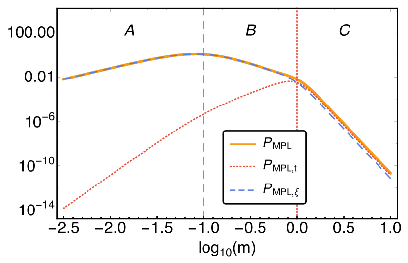
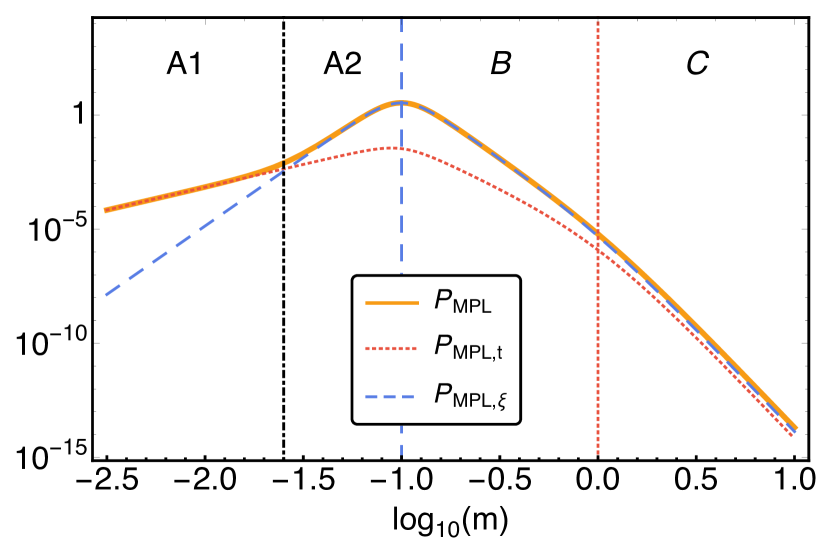
We now turn our attention to the MPL with the base parameter set and investigate the contributions of the two dropout rates to the overall MPL. These are shown in figure 3. Due to the multiplicative structure of the MPL with respect to $\hat{g}_{\text{t}}(m)$ and to $\hat{g}_{\text{$\xi$}}(m)$ the overall decay of the MPL for masses greater than the maximum of $m_{\text{St}}$ and $m_{\text{S$\xi$}}$ (i.e. in region C) is with a power law with exponent $\nu_{>}=-\alpha_{\text{t}}-\alpha_{\text{$\xi$}}-1$, where the $-1$ is due to the Jacobian in the transition from $\log m$ to $m$. It is important to note that this decay also applies to each of the two contributions separately. In region A and B the mass dropout rate dominates the overall behaviour and thus the MPL increases in A with a power law exponent $2\beta_{\text{$\xi$}}-1$ and decreases in B with $-\alpha_{\text{$\xi$}}-1$. The time dropout contribution increases in A with $2\beta_{\text{t}}-1$ and in B with $2\beta_{\text{t}}-\alpha_{\text{$\xi$}}-1$. Interestingly, the time dropout seems to have only a very minor influence on the MPL in regions A and B but its presence shows up in the increased decay in region C.

The situation changes drastically if we make a change in the standard parameter set by exchanging the values of $\alpha_{\xi}$ with $\alpha_{\text{t}}$ and $\beta_{\xi}$ with $\beta_{\text{t}}$: $\alpha_{\text{t}}=3$, $\beta_{\text{t}}=1$, $\alpha_{\text{$\xi$}}=6$, $\beta_{\text{$\xi$}}=3$, and Figure 4 shows the MPL again for the two cases of vanishing time and mass dropout.

Figure 4: The MPL distribution given in eq. (30), is shown for two cases: one in which the mass dropout rate $\hat{k}_{\xi}$ is set to 0 ($\alpha_{\text{$\xi$}}=0$) but the time dropout rate $\hat{k}_{\text{t}}$ is nonzero ($\alpha_{\text{t}}=3$ $\beta_{\text{t}}=1$, and $m_{\text{St}}=10^{0}$)

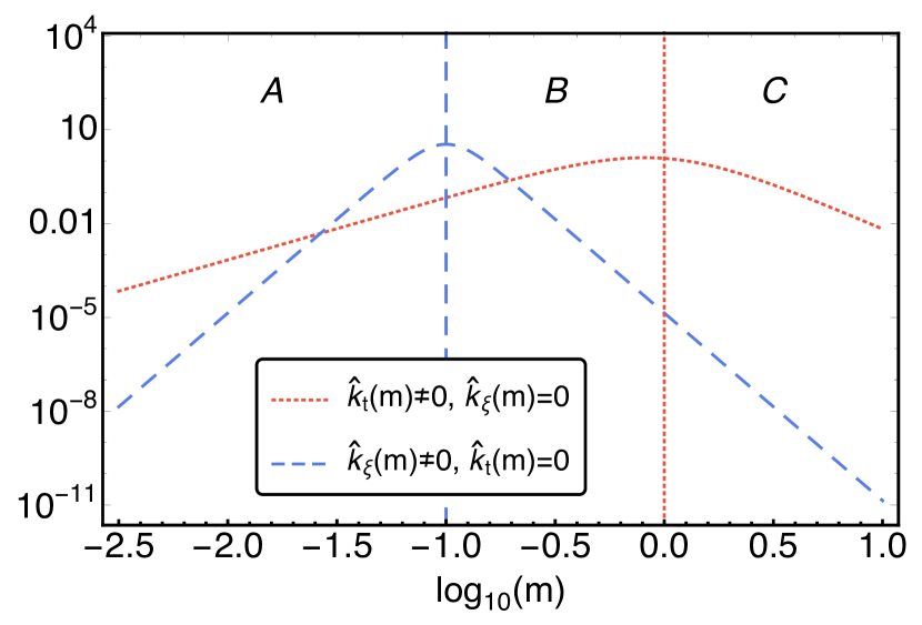
and one in which the time dropout rate $\hat{k}_{\text{t}}$ is set to 0 ($\alpha_{\text{t}}=0$) but the mass dropout rate $\hat{k}_{\text{$\xi$}}$ is nonzero ($\alpha_{\text{$\xi$}}=6$, $\beta_{\text{$\xi$}}=3$, and $m_{\text{S$\xi$}}=10^{-1}$). Here the low and the high mass end of the MPL distribution with $\hat{k}_{\text{t}}(m)=0$ has a steeper increase and decrease, respectively, than for the MPL distribution with $\hat{k}_{\xi}(m)=0$.

If we now combine the two contributions, the MPL shows a distinctly different form than in the standard case as can be seen in figure 5. As the two contributions cross in region A and the mass rate becomes greater than the time rate contribution, region A is split into regions A1 and A2. In A1 the power law increase is with the smaller exponent $2\beta_{\text{t}}-1=1$, while in A2 the mass dropout rate with $2\beta_{\text{$\xi$}}-1=3$ takes over. This is shown in figure 5. In region B we find an exponent $2\beta_{\text{t}}-\alpha_{\text{$\xi$}}-1$ and in C the exponent equals $\alpha_{\text{t}}-\alpha_{\text{$\xi$}}-1$.

Figure 5: $P_{\text{MPL}}$ and the corresponding time term $P_{\text{MPL,t}}$ and mass term $P_{\text{MPL,$\xi$}}$, as given in eq. (30), are shown for the altered standard parameter set ($\alpha_{\text{t}}=3$, $\beta_{\text{t}}=1$, $m_{\text{St}}=10^{0}$, $\alpha_{\text{$\xi$}}=6$, $\beta_{\text{$\xi$}}=3$, and $m_{\text{S$\xi$}}=10^{-1}$). As $P_{\text{MPL}}$ is the sum of $P_{\text{MPL,t}}$, and $P_{\text{MPL,$\xi$}}$, here a complex behaviour of the MPL distribution, with four different regions is found.

4 Illustrative Example: Orion Nebula Cluster IMF

In order to show the implications of our model let us assume that the dropout rate has a second increase due to some global event on "Nebula time“, i.e. it effects all stars in the same fashion as shown in figure 1. Of course Nebula time here is simply a modeling device introduced to illustrate this further increase in the accretion dropout rate, which can in principle occur prior or after the basic mass-related dropout increase. Such a further increase may be due to either another intrinsic mass-related effect or to extrinsic (i.e. non single protostar mass-related) features of the nebula. For example, an extrinsic effect can be that at a time $t_{\text{St}}$ after a molecular cloud starts forming, the nebula may be largely cleared away. Stars that formed early in the history of star formation in the molecular cloud and happen to still be accreting will then face a significant increase in the probability of stopping accretion.

Nebulae where active star formation takes place, are firmly evolving according to common underlying physics. However star forming regions are each unique in the manner of complex systems. Each may develop in completely unique ways within physical law globally, and locally too. Local departures from universality might cancel out in the IMF, or they can be cumulative, leaving distinctive unique global features in the final PDF.

This presents a conundrum for an idealized notion of the IMF that applies to all clusters producing a common result. Each cluster has a unique history that limits the consideration of universal properties. Moreover, young clusters like the ONC have mass distributions that are still forming. Furthermore, there is reason to believe that there is more than one distinct population in play Jerabkova et al. (2019)

The notion of nebula time is a step toward capturing more complex histories and transient features. But the nebula time machinery is far from comprehensive in this regard. It represents a modeling experiment to gain a sense of how the evolution equation approach can be made to capture more subtle structures. Its machinery in this paper still represents a considerable constraint on what forms are possible. Is it flexible enough to match actual data of some kind? To address this question we present an example for the range of possible IMF forms which can be achieved within our modeling approach. In particular we show that the MPL IMF can fit observed IMF data well. This does not constitute a claim that the data in question represents a system with a Nebula time and it does not represent an empirical fit of data. It merely establishes that physically coherent sub-classes of PDFs can effectively match sensible data, giving us clues for next steps of development in the evolution equation approach.

As a basis for this exercise we use data presented by Da Rio et al. (2012) for the Orion Nebula Cluster (here taken from fig. 18 of Da Rio et al. (2012)).

Figure 6: The IMF for the Orion Nebula Cluster as obtained by (Da Rio et al., 2012) is shown together with an appropriately adjusted MPL distribution.

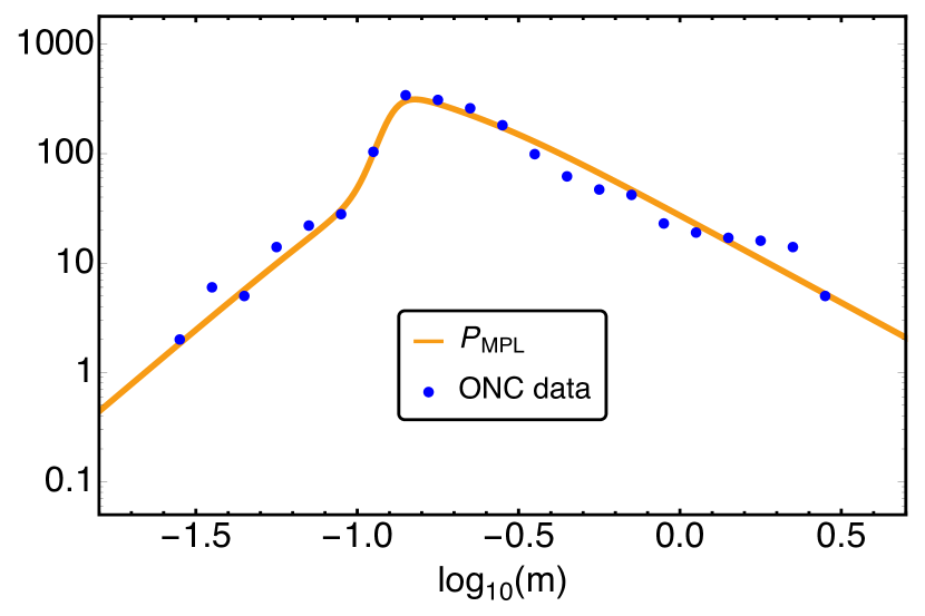
Figure 6 shows a fit for the ONC data of Da Rio et al. (2012) based on the D’Antona & Mazzitelli model. The parameters are $\alpha_{\text{t}}=0.6$, $\beta_{\text{t}}=1.25$, $m_{\text{St}}=10^{-0.72}$, $\alpha_{\text{$\xi$}}=1.0$, $\beta_{\text{$\xi$}}=7.0$, and $m_{\text{S$\xi$}}=10^{-0.9}$. It follows that the exponent $\nu_{>}=-\alpha_{\text{t}}-\alpha_{\text{$\xi$}}-1=-2.6$ for the high mass power law decay is consistent with Kroupa (2002). An interesting observation is that the two dropout masses are only a factor of $10^{0.2}\approx 1.6$ apart.

5 Conclusions

In this model we studied star formation within a dynamical picture based on evolution equations for the probability distribution functions of protostars (still-accreting stars) of a particular mass and of stars that have dropped out of the accretion process. In particular we investigated the properties of IMFs that are generated if the dropout rate increases in two (smeared out) steps. The resulting multi power law IMF is characterized by a power law behaviour for low and high masses, where the respective exponents can be determined in terms of the dropout rates. In the intermediate regime, further power laws with different exponents emerged. For instance, IMFs with three distinct sections can be generated and resemble forms that have been used before in the literature. In this model the dropout rate consists of two parts, one of which describes accretion termination based on star mass, and one which describes accretion termination based on the evolution time; we refer to the latter as a nebula time and it may be associated with processes that starve mass accretion such as outflows or feedback from other stars. The mass growth law is restricted to be exponential, and may be most applicable to late time accretion that leads to intermediate and high mass stars. Future work can explore the low mass accretion rate more realistically. It could also include episodic events of mass growth.

The progress reached in this work lies in the demonstration of the variability of IMFs possible within our approach. Although power laws are generated, the details of the value of particularly the nebula time may vary from one star-forming cluster to another. Hence the physics of star formation may lead to power-laws in the IMF, but leave behind a variety of index values and transition points. A compendium of fits to cluster mass functions reveals a noticeable but not dramatic spread of power laws and transition points (Bastian et al., 2010), but a debate continues as to whether or not this represents universality given the observational uncertainties. Other theoretical models of the IMF such as turbulent fragmentation (Padoan & Nordlund, 2002; Hennebelle & Chabrier, 2008) and ideas such as competitive accretion (Bonnell et al., 1997) rely on specific conditions of molecular gas clouds and turbulence that need to be universal if the IMF is universal, and their dependence on varying initial gas conditions is difficult to model analytically. Our approach is consistent with variability in a manner that may be quantifiable in future work that ties the mass growth law and termination probabilities more closely to physical phenomena. It is also flexible enough to explain multiple mass regions of the IMF and not just the intermediate to high mass tail.

6 Acknowledgements

We thank the referee Hans Zinnecker for his extremely thoughtful comments that helped to improve the manuscript.

References

- Adams & Fatuzzo (1996) Adams F. C., Fatuzzo M., 1996, Astrophys. J., 464, 256
- Bastian et al. (2010) Bastian N., Covey K. R., Meyer M. R., 2010, Annu. Rev. Astron. Astrophys., 48, 339
- Basu & Jones (2004) Basu S., Jones C. E., 2004, Mon. Not. R. Astron. Soc., 347, L47
- Basu et al. (2015) Basu S., Gil M., Auddy S., 2015, Mon. Not. R. Astron. Soc., 449, 2413
- Bonnell et al. (1997) Bonnell I. A., Bate M. R., Clarke C. J., Pringle J. E., 1997, Mon. Not. R. Astron. Soc., 285, 201
- Bonnell et al. (2007) Bonnell I. A., Larson R. B., Zinnecker H., 2007, in Reipurth B., Jewitt D., Keil K., eds, Protostars and Planets V. University of Arizona Space Science Series. The University of Arizona Press, Arizona, US, pp 149–164
- Chabrier (2005) Chabrier G., 2005, in Corbelli E., Palla F., Zinnecker H., eds, Astrophysics and Space Science Library Vol. 327, The Initial Mass Function 50 Years Later. Springer Netherlands, pp 41–50, doi:10.1007/978-1-4020-3407-7_5
- Da Rio et al. (2012) Da Rio N., Robberto M., Hillenbrand L. A., Henning T., Stassun K. G., 2012, Astro. J., 748, 14
- Drass et al. (2016) Drass H., Haas M., Chini R., Bayo A., Hackstein M., Hoffmeister V., Godoy N., Vogt N., 2016, Mon. Not. R. Astron. Soc., 461, 1734
- Hennebelle & Chabrier (2008) Hennebelle P., Chabrier G., 2008, Astrophys. J., 684, 395
- Hennebelle & Chabrier (2009) Hennebelle P., Chabrier G., 2009, Astrophys. J., 702, 1428
- Hoffmann et al. (2018) Hoffmann K. H., Essex C., Basu S., Prehl J., 2018, Mon. Not. R. Astron. Soc., 478, 2113
- Jerabkova et al. (2019) Jerabkova T., Beccari G., Boffin H. M. J., Petr-Gotzens M. G., Manara C. F., Moroni P. G. P., Tognelli E., Degl’Innocenti S., 2019, arXiv, 1905.06974 [astro-ph.SR], 1
- Kroupa (2001) Kroupa P., 2001, Mon. Not. R. Astron. Soc., 322, 231
- Kroupa (2002) Kroupa P., 2002, Science, 295, 82
- Myers (2011) Myers P. C., 2011, Astrophys. J., 743, 98
- Padoan & Nordlund (2002) Padoan P., Nordlund Å., 2002, Astrophys. J., 576, 870
- Padoan & Nordlund (2004) Padoan P., Nordlund Å., 2004, Astrophys. J., 617, 559
- Shu et al. (1987) Shu F. H., Adams F. C., Lizano S., 1987, Annu. Rev. Astron. Astrophys., 25, 23
- Suárez et al. (2019) Suárez G., Downes J. J., Román-Zúñiga C., no B., Petr-Gotzens M. G., Vivas K., 2019, arXiv, 1903.05739v1 [astro-ph.SR], 1
- Zinnecker (1982) Zinnecker H., 1982, Ann. N. Y. Acad. Sci., 395, 226
- Zinnecker (1984) Zinnecker H., 1984, Mon. Not. R. Astron. Soc., 210, 43