Corona-Heated Accretion-disk Reprocessing (CHAR): A Physical Model to Decipher the Melody of AGN UV/optical Twinkling

Abstract

Active galactic nuclei (AGNs) have long been observed to “twinkle” (i.e., their brightness varies with time) on timescales from days to years in the UV/optical bands. Such AGN UV/optical variability is essential for probing the physics of supermassive black holes (SMBHs), the accretion disk, and the broad-line region. Here we show that the temperature fluctuations of an AGN accretion disk, which is magnetically coupled with the corona, can account for observed high-quality AGN optical light curves. We calculate the temperature fluctuations by considering the gas physics of the accreted matter near the SMBH. We find that the resulting simulated AGN UV/optical light curves share the same statistical properties as the observed ones as long as the dimensionless viscosity parameter $\alpha$, which is widely believed to be controlled by magnetohydrodynamic (MHD) turbulence in the accretion disk, is about $0.01$—$0.2$. Moreover, our model can simultaneously explain the larger-than-expected accretion disk sizes and the dependence of UV/optical variability upon wavelength for NGC 5548. Our model also has the potential to explain some other observational facts of AGN UV/optical variability, including the timescale-dependent bluer-when-brighter color variability and the dependence of UV/optical variability on AGN luminosity and black hole mass. Our results also demonstrate a promising way to infer the black-hole mass, the accretion rate, and the radiative efficiency, thereby facilitating understanding of the gas physics and MHD turbulence near the SMBH and its cosmic mass growth history by fitting the AGN UV/optical light curves in the era of time-domain astronomy.

1 Introduction

The ultra-violet (UV) to optical continuum emission of active galactic nuclei (AGNs) is widely believed to be emitted by a geometrically thin but optically thick accretion disk (i.e., the classical standard thin disk, hereafter SSD; see, e.g., Shakura & Sunyaev, 1973; Czerny & Elvis, 1987). The gravitational energy released in the disk is balanced by the blackbody radiative cooling, and the effective temperature decreases with increasing distance from the central supermassive black hole (SMBH). The UV-to-optical emission is a superposition of multi-temperature blackbody radiation. The expected UV-to-optical spectral energy distribution (SED), however, might be altered by additional physical processes, e.g., strong disk winds (e.g., Slone & Netzer, 2012; Laor & Davis, 2014; Li et al., 2019; Sun et al., 2019) or a disk atmosphere (e.g., Hall et al., 2018). Also, for very faint or luminous AGNs, cooling due to advection or photon trapping plays an important role (e.g., Abramowicz et al., 1988; Yuan & Narayan, 2014). In the innermost regions or above the accretion disk, there also exists a hot and optically thin corona which produces hard X-ray emission (e.g., Haardt & Maraschi, 1991; Liu et al., 2002).

UV and optical emission often possesses small-amplitude ($\sim 10\%$ on timescales of a few years) stochastic variability; violent AGN flares are also observed in a small fraction of AGNs (e.g., MacLeod et al., 2016; Yang et al., 2018). The statistical properties of AGN UV and optical stochastic variations have been explored in great detail in many works. The major observational results of these works can be summarized as follows.

1. A damped random walk (DRW) process (whose power spectral density, PSD, $P(f)\propto 1/(f_{0}^{2}+f^{2})$, where $f_{0}=1/\tau$ is the damping frequency) seems to be able to describe AGN UV/optical variability on timescales of months to years (Kelly et al., 2009; MacLeod et al., 2010; Zu et al., 2013). On very short timescales (e.g., days), the observed variability amplitude is lower than the prediction of the DRW model (Mushotzky et al., 2011; Kasliwal et al., 2015; Smith et al., 2018a). On very long timescales (e.g., several decades), the DRW model seems to under-predict the actual variability amplitude (MacLeod et al., 2012; Guo et al., 2017).

2. AGN UV/optical fractional variability amplitude increases with decreasing rest-frame wavelength (i.e., UV emission is more variable than optical emission; see, e.g., MacLeod et al., 2010; Morganson et al., 2014; Sun et al., 2015; Simm et al., 2016; Sánchez-Sáez et al., 2018).

3. AGN UV/optical fractional variability amplitude anti-correlates with AGN luminosity (e.g., MacLeod et al., 2010; Zuo et al., 2012; Morganson et al., 2014; Li et al., 2018; Sun et al., 2018d), the iron strength (i.e., the ratio of optical iron emission to H$\beta$; see, e.g., Ai et al., 2010; Sun et al., 2018d), Eddington ratio (e.g., MacLeod et al., 2010; Zuo et al., 2012; Simm et al., 2016), or additional parameters (e.g., Kang et al., 2018).

4. The damping timescale $\tau$ correlates with AGN luminosity (Sun et al., 2018d), black-hole mass ($M_{\mathrm{BH}}$), or wavelength (MacLeod et al., 2010).

5. AGN color tends to follow a bluer-when-brighter pattern (e.g., Ruan et al., 2014). The bluer-when-brighter behavior seems to be more evident on timescales of weeks to months rather than on timescales of years (Sun et al., 2014).

6. Variations in different bands are well coordinated. Changes of short-wavelength emission lead those of long-wavelength emission (e.g., Sergeev et al., 2005; Fausnaugh et al., 2016; Jiang et al., 2017; Homayouni et al., 2019; Cackett et al., 2018; Kokubo, 2018; McHardy et al., 2018; Mudd et al., 2018; Yu et al., 2018; Edelson et al., 2019). Current observations have a broad diversity of measured time lags beyond the SSD theory: some AGNs have time lags that are about three times larger than the flux-weighted light-travel time delays of the SSD theory. The time lags between X-ray and UV emission can be even about ten times larger than the expectations of the SSD theory, and their correlations often seem to be weak (Edelson et al., 2019).

7. AGN microlensing observations also suggest that the accretion-disk sizes are larger than the flux-weighted radii of the SSD theory (e.g., Morgan et al., 2010; Cornachione et al., 2019).

Variations in the UV-to-optical bands might be caused by the reprocessing of variable X-ray emission (Collin-Souffrin, 1991; Krolik et al., 1991). In the X-ray reprocessing model, as the variable X-ray emission propagates to the disk surface, it is absorbed by the cold disk surface. It is then reprocessed immediately in the UV/optical bands (see Eq. 1 and Section 2.1). That is, UV/optical emission is expected to vary in response to X-ray light curves after a light-travel time delay; the time delay increases with increasing wavelength since the effective temperature anti-correlates with radius. The UV/optical inter-band correlations and time lags are indeed observed (see the observational fact # 6). They can be used to probe the temperature profile and to constrain the fundamental physical processes of the accretion disk (e.g., Lawrence, 2018). However, the expected tight correlations between X-ray and UV/optical emission are not observed at least for some AGNs (for a summary, see Edelson et al., 2019).

AGN broad emission lines (BELs) arise from Doppler-broadened line emission from gas clouds in the broad line region (BLR); these BLR gas clouds are photoionized by the extreme UV (EUV) emission. BELs are also expected to respond to EUV emission after a light-travel time delay; the time delay can probe the spatial structure of BLR (i.e., Reverberation Mapping, hereafter RM; Blandford & McKee, 1982). The EUV variations are not monitored for most RM AGNs; instead, the time lags between BELs and the nearby UV/optical continua are measured. The underlying assumptions are the following: first, the EUV and the nearby UV/optical emission is tightly correlated; second, the time lags between EUV and the nearby UV/optical emission are negligible with respect to the time delays of BELs. The first assumption is probably robust since the tight correlations between BELs and the nearby UV/optical continua are indeed observed (for exceptions, see, e.g., Goad et al., 2016). In addition, a good correlation between the EUV and the $1350\ \mathrm{\AA}$ UV emission indeed exists for NGC 5548 (see Figures 3 & 4 of Marshall et al., 1997). The second assumption may require some attention (e.g., Vestergaard, 2019) since the inter-band time lags are larger than the expectations of the SSD theory for at least some AGNs (see observational fact # 6). Nevertheless, the distance of the BLR to the central SMBH was measured for some AGNs with diverse properties (e.g., Bentz et al., 2009; Du et al., 2016; Grier et al., 2017, 2019), which enables us to estimate $M_{\mathrm{BH}}$ of non-local SMBHs (for recent reviews, see, e.g., Shen, 2013; Peterson, 2014). Therefore, exploring AGN UV/optical variability is of fundamental importance to our understanding of black-hole accretion and our improvement of $M_{\mathrm{BH}}$ measurements.

In the era of time-domain astronomy, large time-domain surveys like LSST (Ivezić et al., 2019) will offer a tremendous amount of AGN variability data (e.g., Brandt et al., 2018). These data can refine the observational conclusions summarized above, help constrain accretion disk models, and obtain AGN physical parameters. These goals can be achieved if we correctly understand the physical origin of AGN UV/optical variability (rather than adopting more complicated empirical stochastic models; Vio et al., 2005).

A few models have been proposed to explain AGN UV/optical variability (for a brief discussion, see, e.g., Czerny et al., 2004; Czerny, 2006). For instance, global (Li & Cao, 2008; Liu et al., 2016) or local (Lyubarskii, 1997) accretion-rate fluctuations might induce the observed UV/optical variations. However, the timescale for the accretion rate to change is the viscous timescale, which is $\gtrsim 100$ yr for the UV/optical emission regions; therefore, this timescale is much longer than our current observations. Instead, local temperature fluctuations (Kelly et al., 2009), which should happen on a much shorter timescale, the thermal timescale (see also Eq. 12), are suggested to be responsible for UV/optical variability. The temperature fluctuations are often assumed to follow the DRW process (e.g., Dexter & Agol, 2011). Such a temperature fluctuation model (with further modifications; see Cai et al., 2016) has the potential to explain the bluer-when-brighter tendency and its timescale dependence. However, this model cannot explain the inter-band correlations (e.g., Kokubo, 2015). Cai et al. (2018) suggested that there are fast-propagating temperature fluctuations (possibly caused by strong outflows or variability in corona; the detailed physical mechanism remains unclear) in the accretion disk. By again assuming that the resulting temperature fluctuations follow the DRW process, they constructed a model to explain the larger-than-expected inter-band time lags in several nearby AGNs. The assumption of DRW-fluctuations in Dexter & Agol (2011) and Cai et al. (2018) is mostly motivated by observations rather than directly by the gas physics of matter near the central SMBH.

The timescale problem can also be avoided by considering X-ray reprocessing because of the following reasons. First, the X-ray emission regions are expected to be compact, and the relevant timescales should be very short. Second, the (variable) hard X-ray photons should be absorbed in the surface layer of the thin cold accretion disk, and the corresponding response timescale is extremely small (Czerny, 2006). However, the expected inter-band time lags are too small to be consistent with observations (see observational fact # 6) although this discrepancy could be resolved by adding an additional ingredient, e.g., non-blackbody emission (Hall et al., 2018) or strong winds (Sun et al., 2019). Moreover, the simplest X-ray reprocessing model also predicts too much short-term variability (note that this inconsistency can be solved by replacing the X-ray corona with a UV torus; Gardner & Done, 2017). There are additional fundamental observational challenges. According to the simplest X-ray reprocessing model, the light curves at all different wavelengths should vary in a very similar way. This prediction is inconsistent with the observational facts # 2, 4, and 5 (Zhu et al., 2018). Meanwhile, as mentioned above, the expected tight correlations between X-ray and UV/optical emission are not observed at least for some AGNs (for a summary, see Edelson et al., 2019). Last but not least, there is a long-standing energy-budget problem (e.g., Clavel et al., 1992; Dexter et al., 2019) in the X-ray reprocessing model. According to this model, the X-ray luminosity should be comparable to the internal dissipation rate to produce the observed fractional variability of $10\%\sim 30\%$ in the UV/optical bands. At least for luminous AGNs, the required X-ray luminosity is likely to be too large to be consistent with X-ray observations (e.g., Just et al., 2007). The energy-budget problem is even more serious for highly variable AGNs (i.e., AGNs with UV/optical fractional variability amplitudes of about several to ten; see, e.g., Dexter et al., 2019). Therefore, the X-ray reprocessing model is unlikely to fully drive AGN UV/optical variability.

In this work, we propose a new model, i.e., Corona-Heated Accretion-disk Reprocessing (hereafter CHAR), to understand AGN UV and optical variability. In this model, the outer ($\gtrsim 10$ Schwarzschild radius) disk and the innermost corona are efficiently coupled via the magnetic field. As the magnetic turbulence/flaring in the corona drives X-ray variability, the same process also changes the accretion-disk heating rate and induces its temperature fluctuations (see Section 2). The energy-budget problem mentioned above might be avoided in our magnetic coupling picture if the corona is radiatively inefficient where most energy is carried by protons rather than electrons, and protons and electrons are decoupled (see e.g., Di Matteo 1998; Różańska & Czerny 2000). If so, only a small fraction of the power of the magnetic flares/turbulence in the corona drives X-ray emission, the remaining of which can affect the disk interior and induce significant UV/optical variability. In our CHAR model, we can determine the statistical properties of temperature fluctuations and AGN UV/optical light curves (the correlation between X-ray and UV/optical variability is briefly discussed in Sections 3.2.3 and 5.2) by considering the thermal-energy conservation law of an AGN accretion disk.

This paper is formatted as follows. In Section 2, we present our model. In Section 3, we demonstrate the results of our CHAR model. In Section 4, we apply our model to explain high-quality Kepler AGN light curves and the multi-wavelength light curves and inter-band time lags of NGC 5548. In Section 5, we discuss the assumptions of our CHAR model, compare our CHAR model with some previous works, and forecast AGN UV/optical variability in the era of time-domain astronomy. Our conclusions are summarized in Section 6. The Schwarzschild radius $R_{\mathrm{S}}\equiv 2GM_{\mathrm{BH}}/c^{2}$, where $G$ and $c$ are the gravitational constant and speed of light, respectively. We adopt a flat $\Lambda$CDM cosmology with $h_{0}=0.7$ and $\Omega_{\rm{M}}=0.3$.

2 The Model

2.1 Model Setup

The outer parts (i.e., $R\gg R_{\mathrm{S}}$) of an accretion disk might receive external illumination via X-ray emission from a hot corona or the FUV emission from the inner (e.g., within $\sim 10R_{\mathrm{S}}$) disk (e.g., Gardner & Done, 2017). A significant fraction of the illuminating emission will be absorbed by the thin surface of the outer accretion disk. In the simplest X-ray reprocessing model (e.g., Starkey et al., 2017), it is often assumed that the absorbed energy is fully re-radiated away locally, i.e., the radiation cooling rate per surface area satisfies the following relation,

$$Q_{\mathrm{rad}}^{-}(t)=2\sigma T^{4}_{\mathrm{eff}}=Q_{\mathrm{vis}}^{+}(t)+Q_{\mathrm{X}}^{+}(t-R_{X}/c)\\ ,$$ (1)

where $\sigma$, $T_{\mathrm{eff}}$, $R_{X}/c$, and $Q_{\mathrm{X}}$ denote the Stefan-Boltzmann constant, the effective temperature, the light-travel time lag between the hot corona/the innermost disk and the outer disk, and the external heating rate due to the X-ray corona, respectively; $R_{X}=\sqrt{H^{2}+R^{2}}$ is the distance to the corona, where $H$ and $R$ are the distance of the corona and disk with respect to the SMBH, respectively. In the lamppost approximation (Cackett et al., 2007), $Q_{\mathrm{X}}=(1-A)L_{\mathrm{X}}H/(2\pi R^{3})$ where $A$ is the albedo of the disk surface. $L_{\mathrm{X}}$ can vary on timescales of days or less since the X-ray external emission is produced in very compact regions (e.g., within $\sim 10R_{\mathrm{S}}$), and various MHD instabilities may occur (Noble & Krolik, 2009). If we neglect possible fluctuations in $Q_{\mathrm{vis}}^{+}$ , $Q_{\mathrm{rad}}^{-}$ should vary in response to $L_{\mathrm{X}}$ after a light-travel time lag. However, this simple model fails to explain many observational facts (see Section 1).

Magnetic fields play a fundamental role in accretion-disk theories since the magnetorotational instability (MRI) is widely believed to be responsible for producing viscosity in the accretion disk and converting gravitational energy into MHD turbulence. Then, the MHD turbulence dissipates and transfers the magnetic energy to heat the gas in the accretion disk, which produces the observed multi-wavelength emission. In the classical $\alpha$-prescription of viscosity (e.g., Shakura & Sunyaev, 1973), it is assumed that MHD turbulence is controlled by the total pressure in the accretion disk. However, recent numerical MHD simulations of accretion disks reveal the opposite behavior, i.e., MHD turbulence controls heat fluctuations in the accretion disk (e.g., Hirose et al., 2009; Jiang et al., 2013) on timescales from the local orbital timescale to hundreds of times of the thermal timescale. Therefore, magnetic fluctuations can drive temperature variations in the accretion disk, which can lead to UV/optical flux flickering in AGNs. However, the magnetic fluctuations at neighboring radii are expected to be nearly independent on timescales much less than the viscous timescales (which is about several hundred years at the optical emission regions). If so, two consequences are expected: first, the UV/optical inter-band correlations should be extremely weak or absent; second, the variability amplitude of UV/optical emission should be small since the observed UV/optical emission is an integration of blackbody radiation of many radii and the integration largely eliminates the flux variability due to the independence of the fluctuations. These predictions are inconsistent with observations (see Section 1).

Figure 1: Illustration of our CHAR model. The accretion disk (gray) and the corona (light blue) are tightly coupled by the magnetic fields (orange curves). Note that the disk might extend to the innermost stable radius; these inner regions have negligible contribution to the UV/optical variability discussed here. MHD fluctuations/flares in the corona can affect disk MHD turbulence and alter the heating rate in the accretion disk. As a result, the disk temperature fluctuates in response to the variable heating rate. The temperature fluctuations can be determined by solving the equation for thermal-energy conservation (i.e., Eq. 3).

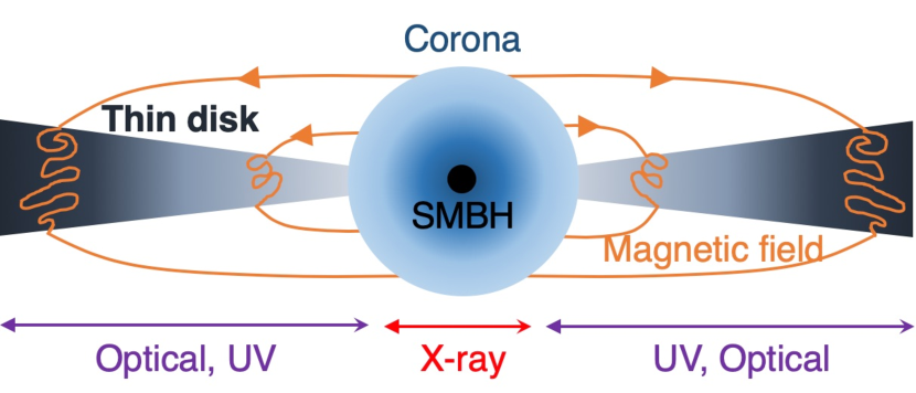
To explain the inter-band correlations/time lags and other observational facts of AGN UV/optical variability, we propose that the X-ray corona and the underlying accretion disk are tightly coupled via the magnetic field (see Figure 1; we defer to Section 5.1 for a detailed discussion of this assumption). As the magnetic field of the corona fluctuates, the magnetic fluctuations (with the power of $Q_{\mathrm{mc}}^{+}$) can also propagate into the accretion disk and induce coherent (i.e., the fluctuations at different radii are correlated) disk magnetic turbulence; the disk magnetic turbulence dissipates and drives a variable heating rate. As a result, the interior structure of the accretion disk should change in response to the variable disk heating rate; the fluctuations of disk structure at different radii are also correlated. Hence, when there are chaotic coronal magnetic fluctuations/flares, we should expect coherent stochastic variations of the observed UV/optical fluxes.

A mathematical description of the above physical picture is complicated and depends on our complete understanding of MHD turbulence. In the absence of such a complete theory of MHD turbulence, we have to make a few assumptions to simplify the above physical picture. Without the corona, the time average (over the viscous timescale) of the vertically integrated heating rate $Q_{\mathrm{vis}}^{+}$ (which is also the dissipation rate of the disk turbulent magnetic power) is

$$\overline{Q_{\mathrm{vis}}^{+}}=\frac{3GM_{\mathrm{BH}}\dot{M}}{4\pi R^{3}}f_{r}\\ ,$$ (2)

where $f_{r}=1-\sqrt{3R_{\mathrm{S}}/R}$ and $\dot{M}$ is the absolute accretion rate. In the presence of a magnetically coupled compact corona, the magnetic fluctuations (with the power per surface area of $Q_{\mathrm{mc}}^{+}$) from the corona propagate into the accretion disk, add to the disk magnetic power, and induce fluctuations of the total magnetic power. The heating rate, which is determined by the dissipation rate of the total magnetic power, is a summation of $Q_{\mathrm{vis}}^{+}$ and $Q_{\mathrm{mc}}^{+}$. To specify the total heating rate, we introduce a new parameter $k=Q^{+}_{\mathrm{mc}}/Q_{\mathrm{vis}}^{+}$, which should be of the order of unity. For simplicity, we may assume that $k$ is constant in $R$; it is straightforward to revise our model to consider the case of $k$ as a function of $R$.

As the total heating rate (which varies in tandem with $Q_{\mathrm{mc}}^{+}$) changes, the AGN accretion disk should be not in vertical hydrostatic equilibrium or thermal equilibrium. The timescale for re-establishing a vertical hydrostatic equilibrium is usually much smaller than the timescale for returning to thermal equilibrium. If we consider the long-term (i.e., much longer than the thermal timescale) variations of the total heating rate, the AGN accretion disk can always adjust its temperature and internal energy to re-establish a new (hydrostatic and thermal) equilibrium state, i.e., Eq. 1 is valid (but $Q_{\mathrm{X}}$ should be replaced by $Q_{\mathrm{mc}}^{+}$). Instead, if we consider the short-term (i.e., shorter than the thermal timescale) variability of the total heating rate, the AGN accretion disk does not have enough time to reach new thermal equilibrium and Eq. 1 is inaccurate.

We assume that an accretion disk can always adjust its vertical structure and scale height to respond to the variable $Q_{\mathrm{mc}}^{+}$ and $Q_{\mathrm{vis}}^{+}$. The temperature fluctuations may be understood by solving the vertically integrated thermal-energy conservation law (see Eq. (4.58) of Kato et al., 2008, for an accretion disk without $Q_{\mathrm{mc}}^{+}$),

$$\frac{\partial E}{\partial t}-(E+\Pi)\frac{\partial\ln\Sigma}{\partial t}+\Pi\frac{\partial\ln H}{\partial t}=Q^{+}_{\mathrm{vis}}+Q_{\mathrm{mc}}^{+}-Q^{-}_{\mathrm{rad}}\\ ,$$ (3)

where $Q^{+}_{\mathrm{vis}}(t)$, $Q_{\mathrm{mc}}^{+}(t-R_{X}/c_{\mathrm{avf}})$, $Q_{\mathrm{rad}}^{-}$(t), $E(t)$, $\Pi(t)$, and $\Sigma(t)$ are the vertically integrated internal viscous heating rate, the additional variable heating rate due to the presence of the corona, the vertically integrated radiative cooling rate, the vertically integrated thermal energy (a summation of both gas and radiation), the vertically integrated pressure (a summation of gas pressure and radiation pressure), and the surface density, respectively. $Q^{+}_{\mathrm{vis}}+Q_{\mathrm{mc}}^{+}$ represent the vertically integrated total heating rate. We assume $Q^{+}_{\mathrm{vis}}$ varies in tandem with $Q_{\mathrm{mc}}^{+}$ after a magnetic field travel time delay, i.e., $Q^{+}_{\mathrm{vis}}(t)=Q_{\mathrm{mc}}^{+}(t-R_{X}/c_{\mathrm{avf}})/k$. The variability propagation speed along the magnetic field is the Alfvén velocity, $c_{\mathrm{avf}}$, which depends on the ratio of the magnetic pressure to the gas density, and can be close to the speed of light for highly magnetized plasma. For simplicity, we assume that the Alfvén velocity of the corona-disk coupling magnetic field is near to the speed of light since the plasma might be highly magnetized. Note that zero advective cooling is assumed, which is a good approximation if the central engine is radiatively efficient.

The solutions of Eq. 3 and the expressions for $Q^{-}_{\mathrm{rad}}$, $E$, $\Pi$, and $\Sigma$ (which are functions of both time $t$ and radius $R$), which describe the temperature fluctuations (and therefore determine UV/optical light curves), depend on the accretion disk model. Here we consider the thin disk model of Shakura & Sunyaev (1973) with minimum modifications according to MHD simulations. We choose the thin-disk model for the following reasons. First, the thin-disk model can well fit the SEDs of some AGNs with X-shooter observations (Capellupo et al., 2015). Second, the disk-instability model for dwarf-novae and low-mass X-ray binary transients, which is built upon the thin-disk model, is widely adopted to adequately explain the outbursts of these systems and constrain the viscosity (e.g., Dubus et al., 2001; Lasota, 2001). The expressions for $Q_{\mathrm{rad}}^{-}$  $E$, $\Pi$, and $\Sigma$ are summarized as follows (for a complete discussion, we refer to Section 4.4.1 of Kato et al., 2008). The pressure scale height can be determined by

$$\Omega^{2}_{\mathrm{K}}H^{2}=\frac{\Pi}{\Sigma}\\ ,$$ (4)

The vertically integrated pressure, $\Pi$, is

$$\Pi=\Pi_{\mathrm{gas}}+\Pi_{\mathrm{rad}}=\frac{2\kappa_{\mathrm{B}}}{m_{\mathrm{p}}}\Sigma T_{\mathrm{c}}+\frac{2aT^{4}_{\mathrm{c}}}{3}H\\ ,$$ (5)

where $\kappa_{\mathrm{B}}$, $m_{\mathrm{p}}$, $a$, and $T_{\mathrm{c}}$ are the Boltzmann constant, the proton mass, the radiation constant, and the inner temperature of the accretion disk, respectively. It is often convenient to define $\beta\equiv\Pi_{\mathrm{gas}}/\Pi$. The vertically integrated thermal energy, $E$, is simply

$$E=E_{\mathrm{gas}}+E_{\mathrm{rad}}=\frac{\beta\Pi}{\gamma-1}+3(1-\beta)\Pi\\ ,$$ (6)

where $\gamma=5/3$ is the ratio of Specific Heat. The vertically integrated radiative cooling is

$$Q_{\mathrm{rad}}^{-}=\frac{8acT_{\mathrm{c}}^{4}}{3\tau_{\mathrm{op}}}=2\sigma T_{\mathrm{eff}}^{4}\\ ,$$ (7)

where $\tau_{\mathrm{op}}$ is optical depth. Optical depth $\tau_{\mathrm{op}}$ is

$$\tau_{\mathrm{op}}=\frac{1}{2}(\kappa_{\mathrm{es}}+\kappa_{0}\rho T_{\mathrm{c}}^{-3.5})\Sigma\\ ,$$ (8)

where $\kappa_{\mathrm{es}}=0.4\ \mathrm{cm^{2}g^{-1}}$, and $\kappa_{0}=6.4\times 10^{23}\ \mathrm{cm^{5}g^{-2}K^{7/2}}$ are the opacity due to electron scattering and free-free absorption, respectively. The total opacity is usually dominated by electron scattering at radii not larger than $\sim 1000\ R_{\mathrm{S}}$.

If we focus on timescales smaller than the viscous timescale, the surface density $\Sigma$ can be regarded as constant in time. Combining Eqs. 3-6, we can obtain

$$C(\beta)\frac{\partial\ln T_{\mathrm{c}}}{\partial t}=\frac{Q_{\mathrm{vis}}^{+}}{\Pi}+\frac{Q_{\mathrm{mc}}^{+}}{\Pi}-\frac{Q_{\mathrm{rad}}^{-}}{\Pi}\\ ,$$ (9)

where $C(\beta)$ is a function of $\beta$,

$$C(\beta)=\Bigg{\{}12(1-\beta)+\frac{\beta}{\gamma-1}+\frac{(4-3\beta)^{2}}{1+\beta}\Bigg{\}}\\ .$$ (10)

In this work, we do not consider any independent non-coherent magnetic fluctuations in the accretion disk. Such independent fluctuations are indeed found in accretion-disk MHD shearing-box simulations (e.g., Hirose et al., 2009; Jiang et al., 2013). The observed AGN luminosity is an integration of blackbody radiation of numerous (of the order of $\gtrsim 10^{2}$) shearing-boxes; the integration eliminates the variability of AGN luminosity due to the independent magnetic fluctuations.

2.2 General Remarks

Some general features can be inferred from Eq. 9. It is convenient to define the so-called “thermal timescale”, i.e.,

$$\tau_{\mathrm{TH}}\equiv\frac{\overline{E}_{\mathrm{gas}}}{\overline{Q}^{+}_{\mathrm{vis}}}\equiv\frac{\overline{\beta}}{\gamma-1}\frac{\overline{\Pi}}{\overline{Q}^{+}_{\mathrm{vis}}}\\ ,$$ (11)

where $\overline{E}_{\mathrm{gas}}$, $\overline{Q}^{+}_{\mathrm{vis}}$, $\overline{\beta}$, and $\overline{\Pi}$ denote the internal energy of the gas, the viscous heating rate, the ratio of gas pressure to total pressure, and the total pressure of a steady solution of Eq. 9. According to the $\alpha$-prescription of viscosity (Shakura & Sunyaev, 1973) and Eq. 11,

$$\tau_{\mathrm{TH}}\sim\frac{1}{\alpha\Omega_{\mathrm{K}}}\propto\alpha^{-1}\lambda^{2}((k+1)\dot{M})^{0.5}\propto\alpha^{-1}\lambda^{2}L_{\mathrm{bol}}^{0.5}\\ ,$$ (12)

where $\alpha$, $\lambda$, and $L_{\mathrm{bol}}$ are the dimensionless viscous parameter, wavelength, and bolometric luminosity, respectively. This scaling relation can be derived as follows. In the steady state, the effective temperature profile is (combining Eqs. 2, 3, and 7 and neglecting time variability), $\overline{T}_{\mathrm{eff}}=(3(k+1)GM_{\mathrm{BH}}\dot{M}/(8\pi\sigma kR^{3}))^{1/4}$. For a given wavelength ($\lambda$), its emission region can be estimated by setting $k_{\mathrm{B}}\overline{T}_{\mathrm{eff}}=hc/\lambda$, where $h$ and $c$ are the Planck constant and the speed of light, respectively. Therefore, it is straightforward to show that $\tau_{\mathrm{TH}}\propto\alpha^{-1}\lambda^{2}[(k+1)\dot{M}]^{0.5}\propto\alpha^{-1}\lambda^{2}L_{\mathrm{bol}}^{0.5}$ since the bolometric luminosity $L_{\mathrm{bol}}\propto(k+1)\dot{M}$ (i.e., by integrating the summation of $Q_{\mathrm{vis}}^{+}$ and $Q_{\mathrm{mc}}^{+}$ over the entire disk).

In a steady state, we have $\overline{Q}^{+}_{\mathrm{mc}}=\overline{Q}^{+}_{\mathrm{vis}}/k$ and $\overline{Q}^{-}_{\mathrm{rad}}=\overline{Q}^{+}_{\mathrm{vis}}+\overline{Q}^{+}_{\mathrm{mc}}$. We can then rewrite Eq. 9 as

$$C(\beta)\frac{\partial\ln T_{\mathrm{c}}}{\partial x}=\frac{\overline{\beta}}{\gamma-1}\frac{f_{\mathrm{vis}}^{+}}{f_{\Pi}}+\frac{\overline{\beta}\ k}{\gamma-1}\frac{f_{\mathrm{mc}}^{+}}{f_{\Pi}}-\frac{\overline{\beta}(k+1)}{\gamma-1}\frac{f_{\mathrm{rad}}^{-}}{f_{\Pi}}\\ ,$$ (13)

where $x=t/\tau_{\mathrm{TH}}$, $f_{\mathrm{vis}}^{+}=Q_{\mathrm{vis}}^{+}/\overline{Q}^{+}_{\mathrm{vis}}$, $f_{\Pi}=\Pi/\overline{\Pi}$, $f_{\mathrm{mc}}^{+}=Q_{\mathrm{mc}}^{+}/\overline{Q}^{+}_{\mathrm{mc}}$, and $f_{\mathrm{rad}}^{-}=Q_{\mathrm{rad}}^{-}/\overline{Q}^{-}_{\mathrm{rad}}$, respectively. Since $Q_{\mathrm{vis}}^{+}$ varies in lockstep with $Q_{\mathrm{mc}}^{+}$, we expect $f_{\mathrm{vis}}^{+}\equiv f^{+}_{\mathrm{mc}}$. Eq. 13 can be revised as

$$f_{\Pi}C(\beta)\frac{\partial\ln T_{\mathrm{c}}}{\partial x}=\frac{\overline{\beta}\ (k+1)}{\gamma-1}(f_{\mathrm{mc}}^{+}-1)-\frac{\overline{\beta}(k+1)}{\gamma-1}(f_{\mathrm{rad}}^{-}-1)\\ .$$ (14)

Note that both $f_{\mathrm{rad}}^{-}$ and $f_{\Pi}$ are functions of $T_{\mathrm{c}}$. For instance, let us consider $T_{\mathrm{c}}=\overline{T}_{\mathrm{c}}(1+\delta T)$ with $\delta T\ll 1$. According to Eq. 7, $f_{\mathrm{rad}}^{-}=(1+4\delta T)$. For gas-pressure dominated regions (i.e., $\beta\simeq 1$), $f_{\Pi}=(1+\delta T)$ (see Eq. 5); for radiation-pressure dominated regions ($\beta\simeq 0$), $f_{\Pi}=(1+8\delta T)$ (see Eqs.  4 and 5).

The second term in the right-hand side of Eq. 14 can be regarded as a damping term. We use $\overline{T}_{\mathrm{c}}$ to represent the inner temperature of a steady solution of Eq. 9. Suppose that $T_{\mathrm{c}}>\overline{T}_{\mathrm{c}}$, then $f_{\mathrm{rad}}^{-}>1$, and the thermal-energy conservation law acts in such a way to reduce $T_{\mathrm{c}}$ until $T_{\mathrm{c}}=\overline{T}_{\mathrm{c}}$ (i.e., the thermal equilibrium is re-established); the reverse is also true. The characteristic timescale of this adjustment is $\sim\tau_{\mathrm{TH}}$.

The first term in the right-hand side of Eq. 14 acts as random fluctuations if $Q_{\mathrm{mc}}^{+}$ suffers from stochastic fluctuations. Therefore, Eq. 14 indicates that the inner temperature $\ln T_{\mathrm{c}}$ is expected to vary stochastically with a damping process, which is similar to observed quasar light curves. The damping timescale is roughly $\tau_{\mathrm{TH}}$. In fact, since Eq. 14 is (nearly) $\tau_{\mathrm{TH}}$-scale-invariant, we also expect statistical properties of $\ln T_{\mathrm{c}}$ fluctuations in AGNs with the same $k$ are similar if the relevant timescales are in units of $\tau_{\mathrm{TH}}$ (Figure 15; see Section 3.3.3).

3 Results

Throughout Section 3, the wavelengths and timescales of quasar features are always in the rest-frame, unless otherwise specified.

3.1 Model Parameters

To understand the temperature fluctuations, we perform numerical calculations. First, we must specify the variability behavior of $Q_{\mathrm{mc}}^{+}$ (which is presumably produced within $\sim 10\ R_{\mathrm{S}}$). Theoretical considerations show that uncorrelated fluctuations at different radii which propagate inward result in accretion-power fluctuations in the innermost regions, and the PSD of the fluctuations is $\propto 1/f$ (e.g., Lyubarskii, 1997; Lin et al., 2016). Three-dimension general relativistic MHD simulations (Noble & Krolik, 2009) also suggest that the PSD of the corona-energy dissipation is $\propto 1/f$. Therefore, we also adopt the $1/f$ law as the PSD of $Q_{\mathrm{mc}}^{+}$. Other PSDs of $Q_{\mathrm{mc}}^{+}$ are possible if the fluctuations at different parts of the corona are not uncorrelated. Our model can easily be generalized to address other PSDs. The probability density distribution (PDF) of $Q_{\mathrm{mc}}^{+}$ is assumed to be log-normal (e.g., Uttley et al., 2005). For illustrative purposes, we fix the fractional variability amplitude of $Q_{\mathrm{mc}}^{+}$, $\delta_{\mathrm{mc}}$, to be $10\%$ on timescales of $10^{5}$ days in Section 3; our calculations can be easily generalized to consider a larger/smaller variability amplitude.

Table 1: Model parameter

Case	$M_{\mathrm{BH}}$	$\dot{m}$	$L_{\mathrm{bol}}$
	$M_{\odot}$		($\mathrm{erg\ s^{-1}}$)
(1)	(2)	(3)	(4)
A	$10^{8}$	$0.1$	$2.5\times 10^{45}$
B	$10^{8}$	$0.3$	$7.6\times 10^{45}$
C	$10^{7}$	$0.1$	$2.5\times 10^{44}$
D	$5\times 10^{7}$	$0.2$	$2.5\times 10^{45}$

Note. — Notes. (1) Case. (2) The black hole mass. (3) The dimensionless accretion rate $\dot{m}=\dot{M}/\dot{M}_{\mathrm{Edd}}$, where $\dot{M}_{\mathrm{Edd}}=10L_{\mathrm{Edd}}/c^{2}$. (4) The bolometric luminosity.

We must set the initial conditions for Eq. 14 (or Eq. 9). At time $t=0$, the initial $T_{\mathrm{c}}$ and $T_{\mathrm{eff}}$ are given by the stationary solution of the standard thin accretion disk with additional $Q_{\mathrm{mc}}^{+}$ (i.e., by considering the stationary solution of Eq. 9 and the mass, momentum, and angular-momentum conservation laws; see Section 3.2.1 of Kato et al., 2008). At this stage, three parameters are introduced, i.e., the dimensionless accretion rate $\dot{m}$, $M_{\mathrm{BH}}$, and the viscous parameter $\alpha$.

The inner and outer boundaries of the accretion disk are fixed to be $10R_{\mathrm{S}}$ and $1000\ R_{\mathrm{S}}$, respectively. The viscous parameter $\alpha$ is fixed to be $0.1$. Our main conclusions would not be significantly changed if we adopted other reasonable values of $\alpha$; the only significant change would be the characteristic timescale $\tau_{\mathrm{TH}}$ since this timescale is $\propto 1/\alpha$. $k$ is assumed to be $1/3$; our results remain unchanged if we consider other values of $k$.

3.2 A Starting Case: $M_{\mathrm{BH}}=10^{8}\ M_{\odot}$, $\dot{m}=0.1$

We start by considering an AGN with $M_{\mathrm{BH}}=10^{8}\ M_{\odot}$ and $\dot{m}=0.1$ (hereafter case A). The bolometric luminosity is $L_{\mathrm{bol}}=(1+k)\dot{m}L_{\mathrm{Edd}}=2.52\times 10^{46}\ \mathrm{erg\ s^{-1}}$.

Figure 2: Upper: the logarithmic variable heating rate ($\log Q^{+}_{\mathrm{mc}}$) as a function of time. Middle: the logarithmic inner temperature ($\log T_{\mathrm{c}}$) and effective temperature ($\log T_{\mathrm{eff}}$) at $R_{3000}$ as a function of time. For clarity, we shift $T_{\mathrm{eff}}$ upward by $0.8$ dex. Lower: the simulated light curves for emission at wavelengths $\lambda=3000\ \mathrm{\AA}$ (blue curve) and $\lambda=5100\ \mathrm{\AA}$ (red curve). Compared with $Q_{\mathrm{mc}}^{+}$ , the fast (i.e., short-term) variability in the UV/optical light curves is significantly suppressed.

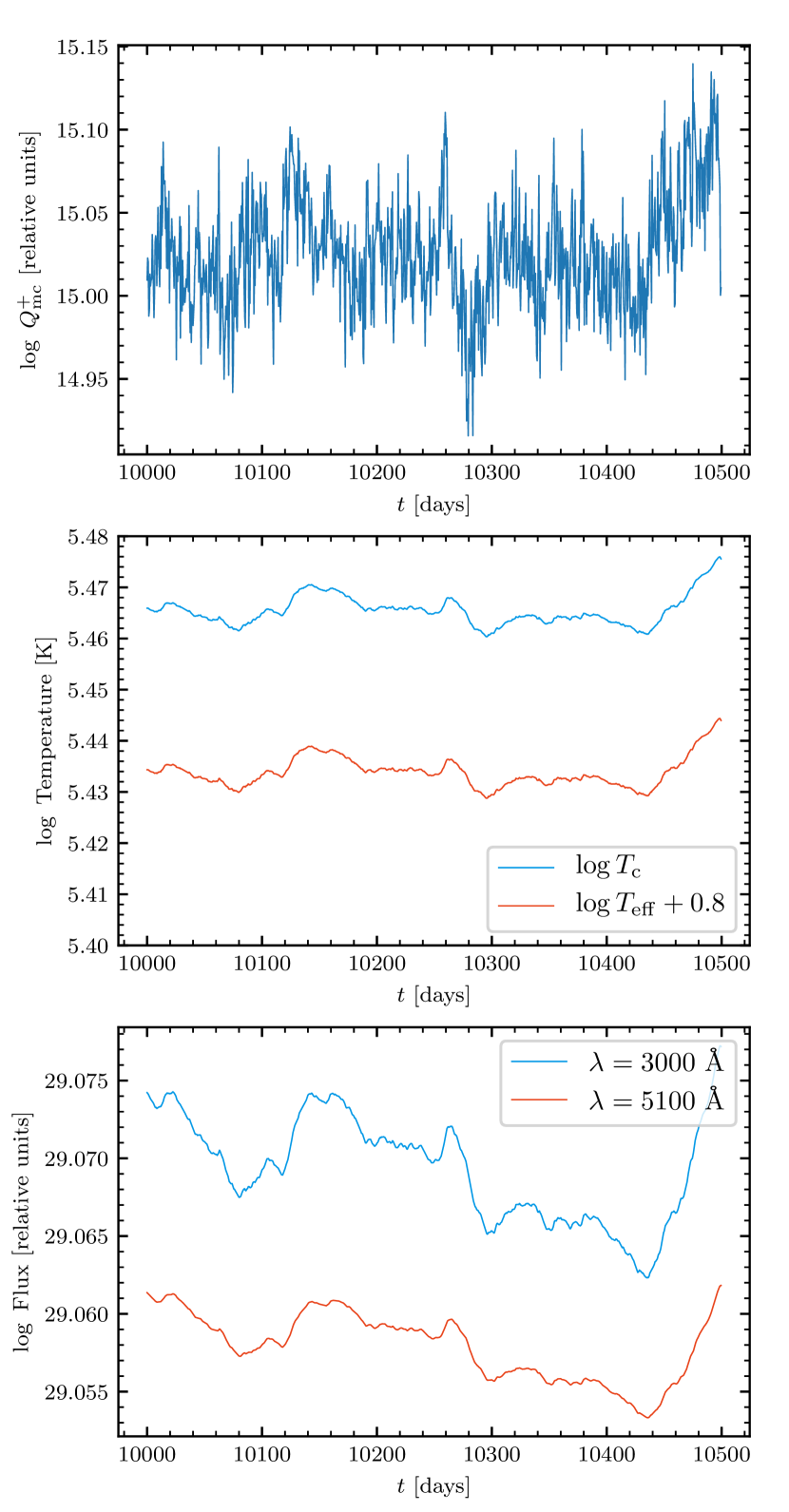
We solve Eq. 9 with a time-step of $0.5$ days to obtain the temporal evolution of $T_{\mathrm{c}}$. The total time length of the light curve of $T_{\mathrm{c}}$ is $10^{5}$ days. The effective temperature, $T_{\mathrm{eff}}$, can be derived by considering Eq. 7 . We then obtain the multi-wavelength light curves by integrating the multi-temperature blackbody emission. The light curves of $Q_{\mathrm{mc}}^{+}$ , $T_{\mathrm{c}}$, $T_{\mathrm{eff}}$, and the $3000\ \mathrm{\AA}$ and $5100\ \mathrm{\AA}$ emission are presented in Figure 2. For illustrative purposes, we show $T_{\mathrm{c}}$ and $T_{\mathrm{eff}}$ at the $3000\ \mathrm{\AA}$ emission characteristic radius ($R_{3000}$; i.e., where $k_{\mathrm{B}}T_{\mathrm{eff}}(R_{3000})=h\lambda/c$ with $\lambda=3000\ \mathrm{\AA}$). At first glance, the fast (i.e., short-term) variability in the light curves of the $3000\ \mathrm{\AA}$ and $5100\ \mathrm{\AA}$ emission is significantly suppressed.

Figure 3: The PSDs of $2.5\log Q^{+}_{\mathrm{mc}}$, $2.5\log T_{\mathrm{c}}$ and $2.5\log T_{\mathrm{eff}}$. For clarity, we shifted the PSD of $2.5\log T_{\mathrm{c}}$ upward by a factor of $10$.

3.2.1 Statistical Properties of Light Curves

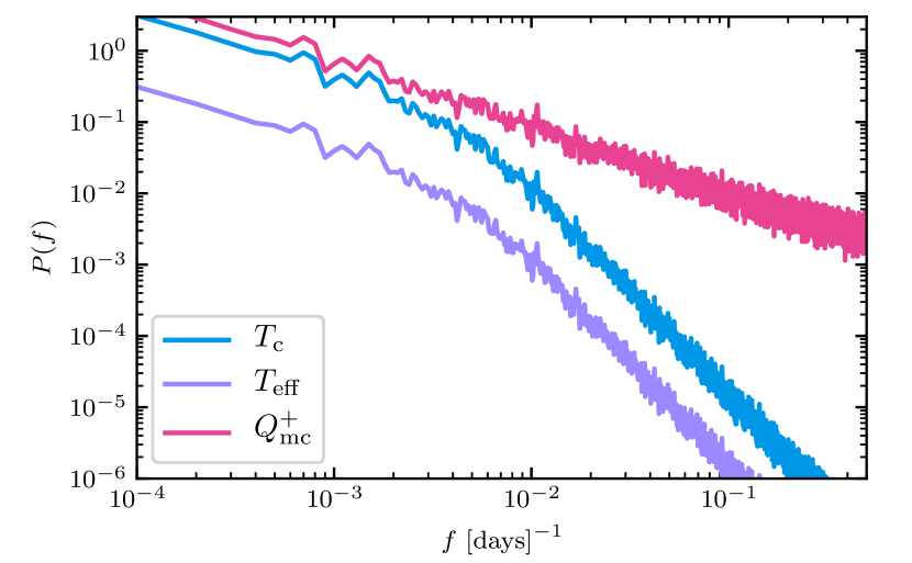
To check the statistical properties of these light curves, we first calculate the PSDs of $2.5\log Q^{+}_{\mathrm{mc}}$, $2.5\log T_{\mathrm{c}}$, and $2.5\log T_{\mathrm{eff}}$. We adopt the Welch method (Welch, 1967) with the light curves broken into ten equal-length segments to calculate the PSDs. The results are shown in Figure 3. At the low-frequency limit, the PSDs of $2.5\log T_{\mathrm{c}}$ and $2.5\log T_{\mathrm{eff}}$ follow that of $Q_{\mathrm{mc}}^{+}$ (i.e., these PSDs follow the $1/f$ shape) . However, at higher frequencies, the PSDs of $2.5\log T_{\mathrm{c}}$ and $2.5\log T_{\mathrm{eff}}$ are steeper (i.e., having less variability power at higher frequencies) than that of $Q_{\mathrm{mc}}^{+}$ .

Figure 4: Upper-left: The PSDs of the $3000\ \mathrm{\AA}$ emission (blue curve) and $2.5\log Q^{+}_{\mathrm{mc}}$ (pink curve). Upper-right: similar to the upper-left one but for the $5100\ \mathrm{\AA}$ emission (red curve). Lower-left: The SF of the $3000\ \mathrm{\AA}$ emission (blue curve). The green dotted curve indicates the DRW fit to the blue curve. Lower-right: similar to the lower-left one but for the $5100\ \mathrm{\AA}$ emission (red curve). The orange dotted curve indicates the DRW fit to the red curve. On long timescales ($\gtrsim 5000$ days), our model is slightly more variable than the predications of the DRW models. However, real observations with limited time durations (typically less than $5000$ days or $\sim 14$ years) cannot probe this deviation. On very short timescales ($\lesssim 10^{2}$ days), the SFs of our model are smaller than those of the best-fitting DRW fits but are very similar to the $\mathrm{SF}\propto\Delta t^{0.8}$ relation (which is the best-fitting model of the best-studied Kepler AGN Zw 229-15; see Kasliwal et al. 2015).

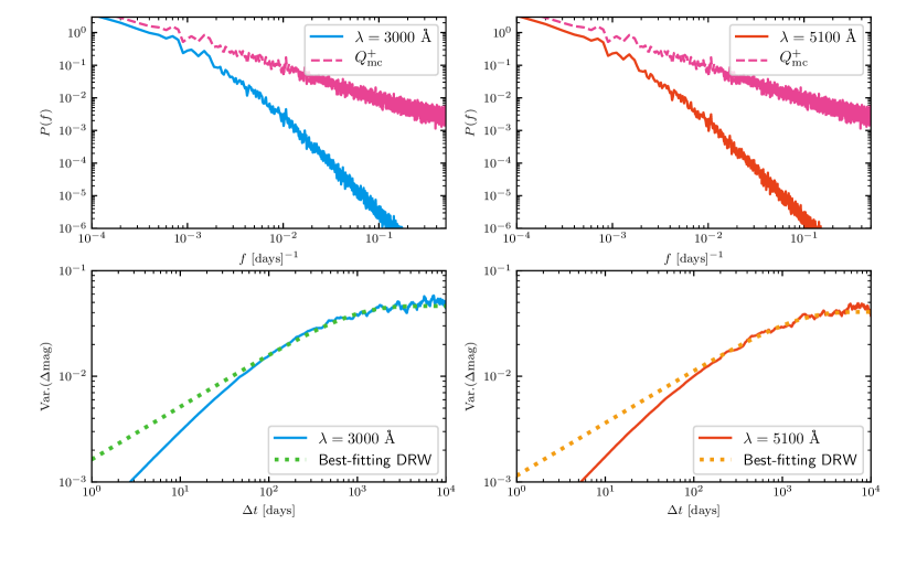
$T_{\mathrm{c}}$ and $T_{\mathrm{eff}}$ are non-observables. Therefore, we now consider the statistical properties of light curves of the $3000\ \mathrm{\AA}$ and $5100\ \mathrm{\AA}$ emission. We again adopt the Welch method to obtain the PSDs. We also measure the structure function (SF) of each light curve; the SF essentially measures the variability amplitude as a function of timescale $\Delta t$. It is argued that the SF is more robust than the PSD for low/irregular-cadence light curves (for a discussion of SF, please refer to Emmanoulopoulos et al., 2010), and it is widely used to quantify AGN UV/optical variability. The SF can be measured by using different statistical estimators (e.g., Sun et al., 2015); each estimator has its own (dis-)advantages (e.g., in terms of treatments of observational uncertainties and outliers). When dealing with simulated data without any measurement errors, we can use any estimator and choose to use the normalized median absolute deviation (NMAD), i.e.,

$$\mathrm{SF}(\Delta t)=1.48\mathrm{Median}(|\Delta m_{i,j}-\mathrm{Median}(\Delta m_{i,j})|)\\ ,$$ (15)

where $\Delta t=|t_{i}-t_{j}|$ is the time separation between two observations (with magnitudes $m_{i}$ and $m_{j}$, respectively) and $\Delta m_{i,j}=m_{j}-m_{i}$.

To calculate the SF, we divide the full light curve of each wavelength into five segments and calculate the SF of each segment. For each wavelength, we then average the five SFs to obtain our final SF.

The PSDs and the SFs of the $3000\ \mathrm{\AA}$ and $5100\ \mathrm{\AA}$ light curves are shown in Figure 4. The SFs show some artificial “peaks” and “dips” on timescales around $10^{4}$ days (i.e., the longest timescale that can be probed by our simulated light curves); these “artificial” features have been identified and discussed by Emmanoulopoulos et al. (2010). Like the PSDs of $T_{\mathrm{c}}$ and $T_{\mathrm{eff}}$, PSDs of the $3000\ \mathrm{\AA}$ and $5100\ \mathrm{\AA}$ light curves are steeper than that of $Q_{\mathrm{mc}}^{+}$ at high frequencies.

Motivated by ground-based observations, it has been proposed that the luminosity variations follow a DRW process, whose SF is (Kelly et al., 2009)

$$\mathrm{SF}(\Delta t)=\hat{\sigma}\sqrt{\tau(1-\exp(-\Delta t/\tau))}\\ ,$$ (16)

where $\hat{\sigma}$ and $\tau$ are the normalization factor and the damping timescale, respectively.

Figure 5: Upper: PSDs of the $3000\ \mathrm{\AA}$ (blue curve) and $5100\ \mathrm{\AA}$ (red curve) emission. Lower: SFs of the $3000\ \mathrm{\AA}$ (blue curve) and $5100\ \mathrm{\AA}$ (red curve) emission. The $3000\ \mathrm{\AA}$ emission is more variable (by a factor of $<2$) than the $5100\ \mathrm{\AA}$ emission.

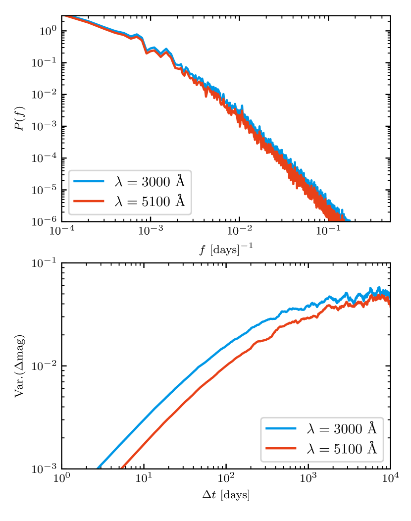
The time duration of observed AGN UV/optical light curves is usually less than $5000$ days (i.e., $\sim 14$ years). To compare our results with the DRW model, we fit Eq. 16 to SFs within timescales smaller than $5000$ days. The best-fitting DRW SFs are included in the lower panels of Figure 4. On timescales of $10^{2}$ up to several thousands of days, the best-fitting DRW model can explain the SFs of our light curves. On shorter timescales, the SFs are steeper than the best-fitting DRW models, i.e., the DRW models over-predict the short-timescale variability. These results are in qualitative agreement with Kepler AGN light curves (e.g., Mushotzky et al., 2011). In fact, the SFs of our model on timescales $\lesssim 10^{2}$ days can be well described by the $\mathrm{SF}\propto\Delta t^{0.8}$ relation, which is the best-fitting model of the best-studied Kepler AGN Zw 229-15 (Kasliwal et al., 2015). The disagreement timescale between the DRW process and our model is $\sim 100$ days in Figure 4. As mentioned in Section 2.2, our model is $\tau_{\mathrm{TH}}$-scale-invariant (see also Section 3.3.3 and Figure 15). If we consider an AGN with $L_{\mathrm{bol}}=6.4\times 10^{43}\ \mathrm{erg\ s^{-1}}$ (i.e., the bolometric luminosity of Zw 229-15; see Barth et al., 2011), its thermal timescale $\tau_{\mathrm{TH}}$ is expected to be a factor of $6.3$ smaller than that of the AGN considered here (see Eq. 12). Therefore, the disagreement timescale between the DRW process and our model should be around $100/6.3=15.8$ days, which is in agreement with that of Zw 229-15 (see Figure 12 in Kelly et al., 2014). Detailed comparisons between our model and the Kepler light curves of Zw 229-15 and several other Kepler AGNs are presented in Section 4.1.

In addition, on timescales $\gtrsim 5000$ days, the best-fitting DRW models under-predict the variability of our light curves. Observationally speaking, there is some indirect evidence that, on long timescales, AGNs are more variable than the predication of the DRW model (MacLeod et al., 2012; Guo et al., 2017).

3.2.2 Wavelength Dependence

We explore the variability amplitude as a function of wavelength and find that the variability amplitude declines with increasing wavelength. An example is presented in Figure 5, which shows the PSDs and SFs of the $3000\ \mathrm{\AA}$ and $5100\ \mathrm{\AA}$ emission. Indeed, the shorter/bluer ($3000\ \mathrm{\AA}$) wavelength light curve is more variable than the longer/redder ($5100\ \mathrm{\AA}$) wavelength one by a factor of $<2$, which is roughly consistent with observations (MacLeod et al., 2012; Sun et al., 2015); the differences are more evident on short timescales. The anti-correlation between the variability amplitude and wavelength can be interpreted as follows. The $3000\ \mathrm{\AA}$ emission has a smaller thermal timescale than that of the $5100\ \mathrm{\AA}$ emission (see Eq. 12). According to Eq. 14, for fixed observing timescale $\Delta t$, the variability amplitude of $\ln T_{\mathrm{c}}(R_{3000})$ is larger than that of $\ln T_{\mathrm{c}}(R_{5100})$ (see Figure 6) since $\Delta x=\Delta t/\tau_{\mathrm{TH}}$ of the former is larger than the latter.

Figure 6: The fractional variability amplitude, $\Delta T_{\mathrm{eff}}/T_{\mathrm{eff}}$, as a function of radius. The blue, red, and purple solid curves are for timescales of one week, one year, and ten years, respectively. The temperature fluctuations are more violent at small radii; this tendency is stronger on short timescales.

3.2.3 Inter-band Cross Correlation

Inter-band cross correlations and time lags are well expected in our model. We use the cross power spectral density (hereafter CPSD; see Section 2.1.2 of Uttley et al., 2014) to explore inter-band correlations and time lags. We again adopt the Welch method to estimate $\mathrm{CPSD}(f)_{1,2}$. $\mathrm{CPSD}(f)_{1,2}$ is usually a complex function. The complex modulus reflects the tightness of the correlation between two light curves; the complex argument indicates the time lag between two light curves.

The tightness of the correlation can be obtained by defining coherence,

$$\Phi(f)_{12}=\frac{\mathrm{abs}(\mathrm{CPSD}(f)_{1,2})^{2}}{P(f)_{1}P(f)_{2}}\\ ,$$ (17)

where $\mathrm{abs}(\mathrm{CPSD}(f)_{1,2})$ is the complex modulus of $\mathrm{CPSD}(f)_{1,2}$ and $P(f)_{1}$ and $P(f)_{2}$ are PSDs of two light curves. We find that $\Phi(f)_{12}\cong 0.99$ (i.e., the correlation is tight).

Figure 7: The frequency-dependent time lag between the $2700\ \mathrm{\AA}$ (close to the central wavelength of the Swift UVW1 band) and the $5400\ \mathrm{\AA}$ (close to the central wavelength of the $V$ band) light curves. The coherence is largely frequency-independent and is $\cong 0.99$ (i.e., the two light curves are tightly correlated). The blue solid line indicates the expected flux-weighted time lag according to the static SSD (Fausnaugh et al., 2016). The dashed line corresponds to the time lag if we increase the flux-weighted time lag by a factor of three. The durations of many high-cadence RM campaigns are $\lesssim 200$ days; therefore, they can only probe variations with $f>0.005\ \mathrm{days}^{-1}$ (the purple vertical line with an arrow).

We then calculate the frequency-dependent time lags from CPSD (see Eq. 10 of Uttley et al., 2014),

$$\tau(f)_{12}=\frac{\mathrm{arg}(\mathrm{CPSD}(f)_{1,2})}{2\pi f}\\ ,$$ (18)

where $\mathrm{arg}(\mathrm{CPSD}(f)_{1,2})$ is the argument of the complex variable $\mathrm{CPSD}(f)_{1,2}$.

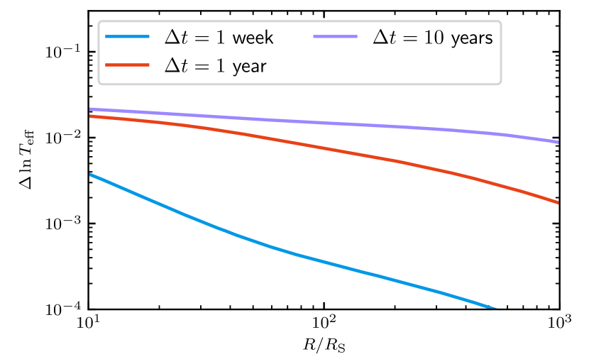
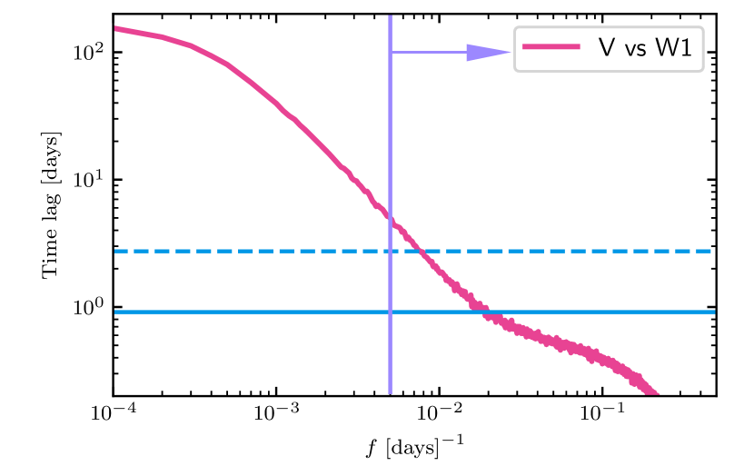
Unlike the simplest X-ray reprocessing model, the inter-band time lags of our CHAR model depend on frequency. The frequency-dependent time lags between the $2700\ \mathrm{\AA}$ (close to the central wavelength of the Swift UVW1 band) and $5400\ \mathrm{\AA}$ (close to the central wavelength of the $V$ band) light curves are presented in Figure 7. To compare with the simplest X-ray reprocessing model, we also show the flux-weighted time lag (Fausnaugh et al., 2016) of a static SSD with the same $M_{\mathrm{BH}}$ and luminosity (hereafter the static SSD time lag). At the high-frequency end (i.e., $f\gtrsim 0.02\ \mathrm{days}^{-1}$), the time lag can be less than the static SSD time lag. The physical reasons are as follows. The measured time lag is an average of time delays of different radii weighted by their surface brightness variations. Unlike the X-ray reprocessing model (which assumes constant fractional temperature fluctuations), the fractional temperature fluctuations in our model anti-correlate with radius on short timescales (see Figure 6) since $\tau_{\mathrm{TH}}\propto R^{\frac{3}{2}}$. That is, the inner-disk regions have larger fractional temperature fluctuations which can induce larger fractional surface brightness variations. Therefore, the weighting factors of inner regions in our model are larger than the flux-weighted case, and our model time lag can be smaller than the static SSD time lag. On frequencies of $\lesssim 0.01\ \mathrm{day}^{-1}$ (which corresponds to the timescales of $\gtrsim 100$ days, i.e., the duration of some high-cadence RM campaigns), the time lag approaches the static SSD time lag. Our model time lag can be significantly larger than the SSD time lag if the frequency is lower than $0.01\ \mathrm{day}^{-1}$. At extremely low frequencies ($f\sim 10^{-4}\ \mathrm{day}^{-1}$), the time lag can be $\sim 200$ days, which is roughly the difference between the thermal timescale of the $2700\ \mathrm{\AA}$ emission and that of the $5400\ \mathrm{\AA}$ emission. Therefore, our model has the potential to explain the observed larger-than-expected time lags in some AGNs.

Figure 8: The relations between the time lag with respect to the $2700\ \mathrm{\AA}$ (close to the central wavelength of the Swift UVW1 band) emission and wavelength for various frequencies. The stars indicate the time lag-wavelength relation for a static SSD.

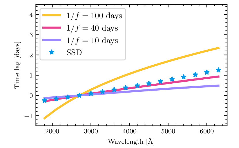
We also calculate the time lag (with respect to the $2700\ \mathrm{\AA}$ emission) as a function of wavelength (see Figure 8). Again, it is shown that lower-frequency components appear to have larger time lags than those of higher-frequency ones; the slope and the normalization of the time lag-wavelength relation also depend on frequency. The observed time lag-wavelength relation is an average of various components with different frequencies. This average process is complicated and depends on the cadence and duration of the RM campaigns. A detailed comparison between our model and the inter-band time lags and multi-wavelength SFs of NGC 5548 is presented in Section 4.2.

We also point out that UV/optical emission and $Q_{\mathrm{mc}}^{+}$ are highly correlated and their time lags can also be much larger than the static SSD time lags, especially on long timescales. It should be noted that these time lags are not identical to the time lags between X-ray and UV emission. This is because there should also be time lags between X-ray and $Q_{\mathrm{mc}}^{+}$. In principle, if the corona can be modeled as an advection dominated accretion flow (e.g., Liu et al., 2002; Yuan & Narayan, 2014), the variability of the X-ray emission can also be obtained by solving the thermal-energy conservation law of the advection dominated accretion flow. The resulting equation is similar to Eq. 3 but with an additional advective cooling term on the right-hand side of Eq. 3. Meanwhile, unlike the SSD, the surface density $\Sigma$ cannot be treated as a constant in time for the advection dominated accretion flow. Therefore, the relation between X-ray luminosity and $Q_{\mathrm{mc}}^{+}$ can be complicated and their variations might not be well coordinated. For instance, an increase in $Q_{\mathrm{mc}}^{+}$ may trigger an increase in $\Sigma$ or the advective cooling without the necessity of invoking an increase in the radiative cooling $Q_{\mathrm{rad}}^{-}$ (i.e., X-ray luminosity). This effect might be responsible for the observed weak correlations between X-ray and UV/optical emission (Edelson et al., 2019). In the future, we plan to model the relation between X-ray luminosity and $Q_{\mathrm{mc}}^{+}$ in detail and determine the relation between UV/optical and X-ray emission.

3.2.4 Microlensing Accretion-Disk Size

As mentioned in Section 1, AGN accretion-disk sizes can be measured via microlensing observations and the resulting accretion-disk sizes are larger than the flux-weighted radii of the static SSD (e.g., Morgan et al., 2010; Cornachione et al., 2019). Our model might be able to resolve this discrepancy.

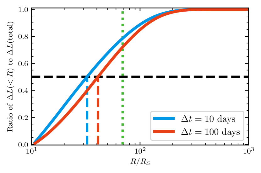
Microlensing observations actually measure the half-light radius of the time-variable AGN emission. Therefore, we follow Tie & Kochanek (2018) and calculate the half-light radius of the time-variable $3000\ \mathrm{\AA}$ emisison as follows. First, we utilize a Taylor expansion to the Planck function and obtain the variation of intensity as a function of radius, i.e.,

$$\Delta B(\lambda,R)=\frac{2hc^{2}}{\lambda^{5}}x\frac{\exp(x)}{(\exp(x)-1)^{2}}\frac{\Delta T_{\mathrm{eff}}}{T_{\mathrm{eff}}}\\ ,$$ (19)

where $\lambda=3000\ \mathrm{\AA}$, $x=hc/(k_{\mathrm{B}}T_{\mathrm{eff}}\lambda)$ and $B(\lambda)$ is the Planck function. Second, for a fixed wavelength, we can calculate the cumulative contribution of $\leq R$ regions to the total variability, i.e.,

$$f_{\mathrm{\Delta L}}(\lambda,R)=\frac{\int_{10R_{\mathrm{S}}}^{R}\Delta B(\lambda,R_{0})R_{0}dR_{0}}{\int_{10R_{\mathrm{S}}}^{10^{3}R_{\mathrm{S}}}\Delta B(\lambda,R_{0})R_{0}dR_{0}}\\ .$$ (20)

Then, the half-light radius, $R_{\mathrm{half}}$, can be calculated by setting $f_{\mathrm{\Delta L}}(\lambda,R_{\mathrm{half}})\equiv 0.5$.

It is evident that $R_{\mathrm{half}}$ should depend on the relation between $\Delta T_{\mathrm{eff}}/T_{\mathrm{eff}}$ and $R$. In the simplest X-ray reprocessing model with a static SSD, it is often assumed that $\Delta T_{\mathrm{eff}}/T_{\mathrm{eff}}$ is constant in $R$. In contrast, our model predicts that $\Delta T_{\mathrm{eff}}/T_{\mathrm{eff}}$ anti-correlates with $R$ on timescales of $\lesssim 10$ years (see Figure 6). That is, our half-light radius is smaller than that of the static SSD (see Figure 9). The flux-weighted radius of our model is similar to that of the static SSD. Therefore, our model has the potential to account for AGN microlensing observations (i.e., the disk size inferred from the half-light radius of a static SSD is larger than the flux-weighted radius). In the future, we plan to convolve our model with gravitational microlensing effects and address the microlensing disk size problem in detail.

Figure 9: The cumulative contribution of $\leq R$ regions to the total variability, $f_{\mathrm{\Delta L}}(\lambda,R)$, as a function of $R$. The blue and red curves correspond to timescales of $10$ days and $100$ days, respectively. The black dashed line indicates $f_{\mathrm{\Delta L}}\equiv 0.5$. The blue and red dashed lines represent the corresponding half-light radii. The green dotted line indicates the half-light radius of the static SSD. In general, the half-light radius of our model is smaller than that of the static SSD.

3.2.5 Color Variability

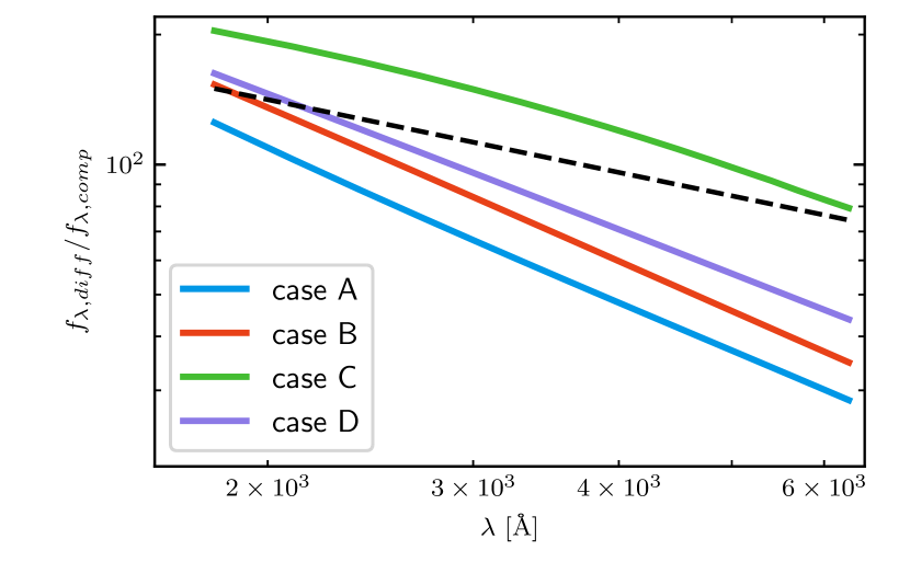
Observationally, AGN color variations show a bluer-when-brighter tendency (Ruan et al., 2014) and this tendency is timescale-dependent (Sun et al., 2014). To check whether our model can predict such a timescale-dependent bluer-when-brighter tendency, we also calculate the color variations of our model. First, we follow the methodology in Section 5 of Ruan et al. (2014) to obtain $1500$ differential spectra. The time separation of two spectra is fixed to be $50$ days. We then scale the $1500$ differential spectra to have the same $3000\ \mathrm{\AA}$ emission and use the geometric mean to obtain the composite differential spectrum, which is shown in Figure 10 (for the differences among cases A, B, C, and D, please see Table 1 and Section 3.3). Our model predicts a bluer-when-brighter power-law spectral variability that is quite similar to the observed one.

Figure 10: The composite differential spectra of our model. The black dashed line corresponds to the observed spectrum with an index of $\Gamma_{\lambda}=-0.56$ (Ruan et al. 2014). The bluer-when-brighter behavior is evident in all cases. The composite differential spectra are also similar to the observed one (Ruan et al., 2014). Cases A-D correspond to different $M_{\mathrm{BH}}$, $\dot{m}$, and $L_{\mathrm{bol}}$ (see Table 1).

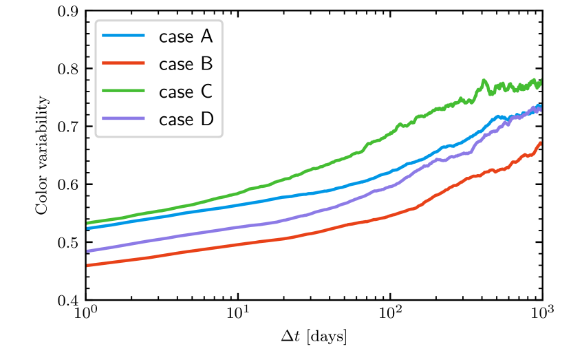
We also calculate the timescale-dependent color variability ($S(\Delta t)$), which measures the ratio of the variations of the shorter-wavelength emission to those of the longer one, by following the methodology in Section 4 of Zhu et al. (2018). The results of the color variability between the $3000\ \mathrm{\AA}$ and $5100\ \mathrm{\AA}$ emission are shown in Figure 11. Indeed, our model also predicts the timescale-dependent bluer-when-brighter behavior, i.e., the bluer-when-brighter behavior is also less prominent on long timescales.

Figure 11: AGN time-dependent color variability of our model. The bluer-when-brighter behavior is more evident on short timescales than on long timescales.

3.3 Parameter Dependence

According to our model, AGN UV/optical variability depends upon AGN physical parameters, namely, $M_{\mathrm{BH}}$ and $\dot{m}$. Therefore, we solve Eq. 9 for four cases (see Table 1).

3.3.1 Dimensionless Accretion-Rate Dependence

To explore the relation between AGN UV/optical variability and $\dot{m}$, we compare case A with two cases (i.e., cases B and D). Cases A and B have the same $M_{\mathrm{BH}}$ but different $\dot{m}$ and $L_{\mathrm{bol}}$. On the other hand, cases A and D share the same $\dot{M}$ and $L_{\mathrm{bol}}$ but different $\dot{m}$ and $M_{\mathrm{BH}}$.

Figure 12: Upper: PSDs of the $3000\ \mathrm{\AA}$ emission for cases A and B. Lower: SFs of the $3000\ \mathrm{\AA}$ emission for cases A and B. For fixed $M_{\mathrm{BH}}$, the variability amplitudes on timescales $\lesssim 10^{3}$ days decrease with increasing $\dot{m}$ or luminosity. This anti-correlation seems to be consistent with the empirical relation of MacLeod et al. (2010) for $\hat{\sigma}$ (see text in Section 3.3.1).

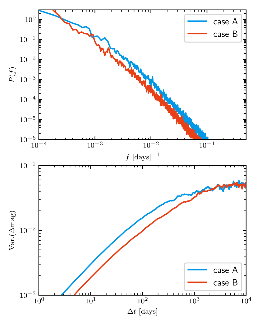
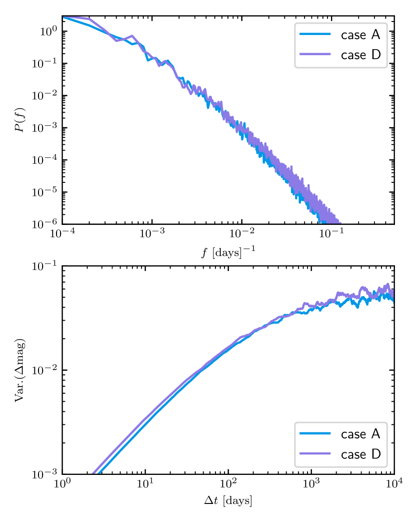
For illustrative purposes, we focus on the statistical properties of the light curves of the $3000\ \mathrm{\AA}$ emission. A comparison between the PSD and SF of case A and those of cases B and D is presented in Figures 12 and 13.

Empirical relations between the observed SFs and AGN physical properties (e.g., luminosity and $M_{\mathrm{BH}}$; for a summary, refer to the Introduction section) have been obtained. One popular empirical relation was reported by MacLeod et al. (2010). It should be noted that such empirical relations might suffer from various statistical biases (for a detailed discussion, see, e.g., Kozłowski, 2017). However, the empirical relation of MacLeod et al. (2010) for the DRW parameter $\hat{\sigma}$ (which determines the SF of a DRW model at timescales that are much smaller than the damping timescale) is likely to be reliable (refer to Figure 1 of Kozłowski, 2017). Therefore, our model predictions are compared with this empirical relation, i.e., $\hat{\sigma}\propto L^{-0.29}M_{\mathrm{BH}}^{0.075}\propto\dot{m}^{-0.29}M_{\mathrm{BH}}^{-0.215}$ (see Section 5.2 of MacLeod et al., 2010).

On timescales of $\lesssim 10^{3}$ days, the $3000\ \mathrm{\AA}$ emission of case A is more variable than that of case B by a factor of about $1.5$. According to the empirical relation of MacLeod et al. (2010) for $\hat{\sigma}$, the SF of case A is expected to be larger than that of case B by a factor of $3^{0.3}\simeq 1.4$. That is, for fixed $M_{\mathrm{BH}}$ (and $Q_{\mathrm{mc}}^{+}$), AGN UV/optical variability decreases with increasing $\dot{m}$ or $L_{\mathrm{bol}}$, and this anti-correlation is roughly consistent with the empirical relation of MacLeod et al. (2010). Cases A and D have similar SFs, i.e., for fixed $L_{\mathrm{bol}}$ (or $\dot{M}$), AGN UV/optical variability is insensitive to $\dot{m}$ or $M_{\mathrm{BH}}$, which is again consistent with the empirical relation of MacLeod et al. (2010).

As for color variability, the differential spectra of cases B and D share a similar shape with that of case A (Figure 10). However, cases B and D show more evident bluer-when-brighter behaviors than case A (Figure 11). That is, the timescale-dependent color variability (bluer-when-brighter) correlates with $\dot{m}$.

Figure 13: Upper: PSDs of the $3000\ \mathrm{\AA}$ emission for cases A and D. Lower: SFs of the $3000\ \mathrm{\AA}$ emission for cases A and D. For fixed $L_{\mathrm{bol}}$, the variability amplitudes are insensitive to $\dot{m}$ or $M_{\mathrm{BH}}$, which is roughly consistent with the empirical relation of MacLeod et al. (2010).

3.3.2 Black-Hole Mass Dependence

To explore the relation between AGN UV/optical variability and $M_{\mathrm{BH}}$, we compare case A with two cases (i.e., cases C and D). Cases A and C have the same $\dot{m}$ but different $M_{\mathrm{BH}}$ and $L_{\mathrm{bol}}$. On the other hand, cases A and D share the same $L_{\mathrm{bol}}$ but different $\dot{m}$ and $M_{\mathrm{BH}}$.

Figure 14: Upper: PSDs of the $3000\ \mathrm{\AA}$ emission for cases A and C. Lower: SFs of the $3000\ \mathrm{\AA}$ emission for cases A and C. For fixed $\dot{m}$, the variability amplitudes on timescales $\lesssim 10^{3}$ days decrease with increasing $M_{\mathrm{BH}}$ or luminosity. This anti-correlation seems to be roughly consistent with the empirical relation of MacLeod et al. (2010) for $\hat{\sigma}$ (see texts in Section 3.3.2).

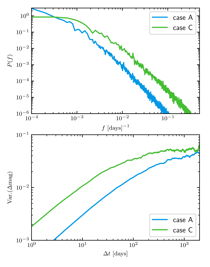
Compared with case A, case C predicts larger variability amplitudes (by a factor of about $2.2$) of the $3000\ \mathrm{\AA}$ emission on timescales of $\lesssim 10^{3}$ days (Figure 14). Therefore, if we control $\dot{m}$ (and $Q_{\mathrm{mc}}^{+}$), AGN UV/optical variability and $M_{\mathrm{BH}}$ are anti-correlated. According to the empirical relation of MacLeod et al. (2010) for $\hat{\sigma}$, the SF of case C is expected to be larger than that of case A by a factor of $10^{0.215}=1.64$, which is smaller than our model prediction by a factor of $2.2/1.64=1.34$. This small discrepancy might be understood as follows. The sample of MacLeod et al. (2010) consists of luminous AGNs while the AGN of case C has a much lower bolometric luminosity ($2.5\times 10^{44}\ \mathrm{erg\ s^{-1}}$). There is some evidence to suggest that the empirical relation of MacLeod et al. (2010) under-predicts the short-term variability amplitudes (by a factor of $\sim 1.3$) of AGNs with relatively low luminosities (see Section 6.1 of Sun et al., 2015).

Instead, if we fix $L_{\mathrm{bol}}$ (i.e., case A vs case D; Figure 13) and $Q_{\mathrm{mc}}^{+}$, there is no strong correlation between AGN UV/optical variability and $M_{\mathrm{BH}}$ which is again consistent with the empirical relation of MacLeod et al. (2010).

As for color variability, the differential spectra of cases C and D share roughly the same shape with that of case A (Figure 10). However, case C (D) shows weaker (stronger) timescale-dependent color variability (bluer-when-brighter) than case A. Therefore, the dependence of AGN timescale-dependent color variability upon $M_{\mathrm{BH}}$ is complicated.

Figure 15: Upper: PSDs of the $3000\ \mathrm{\AA}$ emission for cases A, B, C and D. Lower: SFs of the $3000\ \mathrm{\AA}$ emission for cases A, B, C and D. When $\Delta t$ (the frequency $f$) is expressed in units of the thermal timescale $\tau_{\mathrm{TH}}$ (the thermal frequency $1/\tau_{\mathrm{TH}}$), the PSDs and SFs are nearly the same. The PSDs and SFs depend weakly on $M_{\mathrm{BH}}$ (see case C).

3.3.3 Luminosity Dependence

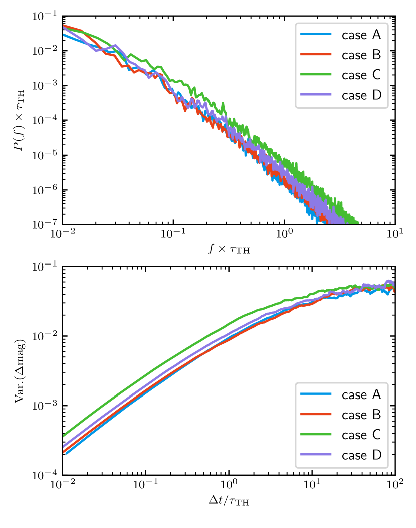
From Sections 3.3.1 and 3.3.2, we can conclude that the PSD and SF of the $3000\ \mathrm{\AA}$ emission depend mostly on AGN luminosity. This tendency can be understood as follows. Eq. 9 is roughly scale-invariant if timescale is in units of the thermal timescale $\tau_{\mathrm{TH}}$ (see Eq. 14) at the $3000\ \mathrm{\AA}$ emission characteristic radius ($R_{3000}$); as mentioned in Section 2.2, $\tau_{\mathrm{TH}}(\lambda)\propto\alpha^{-1}\lambda^{2}L_{\mathrm{bol}}^{0.5}$. Indeed, if we express timescale in units of $\tau_{\mathrm{TH}}$ days, SFs and PSDs of cases A, B and C are quite similar to those of case D (Figure 15). This feature might be responsible for the observed tight correlation between the short-term variability amplitude and AGN luminosity (e.g., MacLeod et al., 2010; Sun et al., 2018d).

It is evident that AGN timescale-dependent color variability (bluer-when-brighter) correlates with $L_{\mathrm{bol}}$ or $\dot{M}$ (i.e., by comparing case A with cases B and C; see Figures 10 and 11).

3.3.4 Inter-band Time Lags and AGN Parameters

Figure 16: The ratios of the frequency-dependent time lags of the UVW1 emission with respect to V-band emission to the static SSD time lags for cases A, B, C, and D. Positive lags indicate that V band lags UVW1 band. For fixed frequency, less luminous sources tend to have larger ratios of measured-to-expected time lags than more luminous ones.

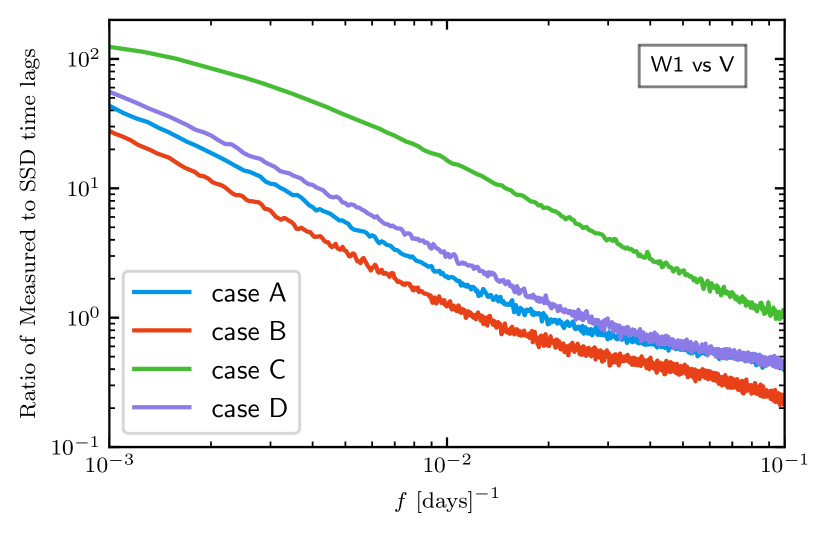
To complete our study, we show the ratios of the time lags between the UVW1-band and the V-band emission to the expectations of a static SSD (with the same $M_{\mathrm{BH}}$ and $\dot{m}$) as a function of frequency for cases A, B, C and D. The results are presented in Figure 16. For fixed observing duration $T_{\mathrm{dur}}=1/f_{\mathrm{dur}}$, the ratio of measured-to-expected time lag of a less luminous AGN is larger than that of a more luminous one (see Figure 16); this can explain observational fact # 6, i.e., the larger-than-expected time lags are observed for several local Seyfert 1 AGNs but not in some more luminous and distant AGNs.

More luminous AGNs tend to have larger thermal timescales (for fixed wavelength and $\alpha$). As a result, the anti-correlation between the fractional variability of the effective temperature and radius is more evident for more luminous AGNs than for less luminous ones. That is, the microlensing accretion-disk size (i.e., the half-light radius of the time-variable emission; see Section 3.2.4) is always over-estimated if the static SSD model is adopted when studying AGN microlensing observations.

4 Confronting Our CHAR Model with Real Observations

We apply our CHAR model to explain two different sets of real observations. First, we consider the long-duration ($\sim 3$ years), high-cadence ($\sim 30$ min) Kepler light curves of three AGNs (namely Zw 229-15, kplr 12158940 and kplr 2694186) which have reliable black-hole mass measurements (Barth et al., 2011; Smith et al., 2018a). Second, we focus on the multi-wavelength light curves of NGC 5548. Throughout Section 4, the wavelengths and timescales of quasar features are always in the observed-frame, unless otherwise specified.

4.1 Kepler Observations

The Kepler space telescope (Borucki et al., 2010) provided extremely high-cadence ($\sim 30$ min) and long-term ($\sim 3$ years) optical light curves for about two dozen AGNs (Smith et al., 2018a). Previous works using such Kepler light curves have revealed that AGN short-term (i.e., $\lesssim 10$ days) variability is inconsistent with the DRW model (Mushotzky et al., 2011; Kasliwal et al., 2015) although this model has been proven to be very useful in describing more limited ground-based data (e.g., Kelly et al., 2009; MacLeod et al., 2010).

We select Kepler AGNs with $M_{\mathrm{BH}}$ estimates (via the reverberation-mapping or the single-epoch virial black-hole mass estimators) from Barth et al. (2011) and Table 1 of Smith et al. (2018a). The $\sim 3$-year Kepler light curves were broken into multiple segments due to instrumental effects. To ensure that the Kepler data can efficiently probe both short-term and long-term variability, we reject AGNs with data from less than $10$ segments. At this stage, five AGNs are selected, namely Zw 229-15, kplr 2694186, kplr 12158940, kplr 12208602, and kplr 9650712. Among them, kplr 12208602 is a radio-loud AGN, i.e., non-disk jet emission might be important; and kplr 9650712 might show a quasi-periodic oscillation signal (Smith et al., 2018b) which is beyond the scope of this work. Therefore, we do not consider these two AGNs, either. Our final sample consists of three sources, Zw 229-15, kplr 2694186 and kplr 12158940.

Table 2: Quality-of-fit assessment for the three AGNs

Name	$\log M_{\mathrm{BH}}$	$\dot{m}$	$\alpha$	$\sigma_{\mathrm{mc}}$	$\chi^{2}/D.O.F.$	$P(\chi^{2}_{\mathrm{mc}}>\chi^{2}_{\mathrm{obs}})$
	$M_{\odot}$
Zw 229-15	7.00	0.034	0.20	0.065	0.53	0.67
			0.01	0.310	3.00	0.05
kplr 12158940	8.04	0.002	0.20	0.084	3.35	0.02
			0.01	0.400	0.23	0.92
kplr 2694186	7.66	0.043	0.20	0.074	2.71	0.03
			0.01	0.640	1.77	0.15

Note. — Notes. (1) Object name. (2) The black hole mass (for Zw 229-15, see Barth et al. (2011); for others, see Smith et al. (2018a)). (3) The dimensionless accretion rate $\dot{m}=\dot{M}/\dot{M}_{\mathrm{Edd}}$, where $\dot{M}_{\mathrm{Edd}}=10L_{\mathrm{Edd}}/c^{2}$. (4) The dimensionless viscosity parameter. (5) The variability amplitude of $Q_{\mathrm{heat}}^{+}$. (6) The ratio of $\chi^{2}$ to degree of freedom (D.O.F., which is $4\times 10^{4}$). (7) $P(\chi^{2}_{\mathrm{mc}}>x)$ is the survival function of the distribution of $\chi^{2}_{\mathrm{mc}}$.

The Kepler light curves of the three AGNs are taken from Chen & Wang (2015). In their work, multiple-quarter light curves are stitched together by considering the PyKE routines kepmask and kepextract (Kinemuchi et al., 2012). Additional CBV (i.e., the cotrending basis vectors) corrections are not applied as such corrections are unlikely to be highly accurate at least for the best-studied source Zw 229-15 (see Figure 27 of Smith et al., 2018a). The adopted light curves are presented in Figure 17.

Figure 17: The Kepler light curves for the three Kepler AGNs with high-quality data (with a timespan of $\sim 3$ years and a cadence of $\sim 30$ min) and $M_{\mathrm{BH}}$ estimates. The typical fractional simple aperture photometry (SAP) flux uncertainty is $\sim 0.08\%$. The SAP flux is in units of count rate and the bandpass is from $4200$ Å to $9000$ Å.

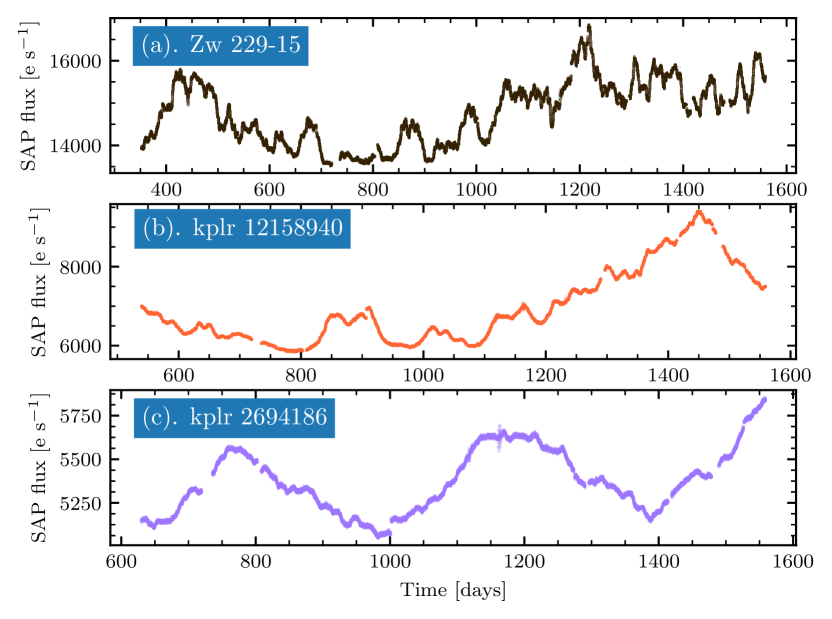
For each source, $M_{\mathrm{BH}}$ is fixed to the observed value; $\dot{M}$ is chosen to match the observed luminosity at rest-frame $\lambda=5100$ Å; and $\delta_{\mathrm{mc}}$ is adjusted such that the predicted SF equals the observed one at $\Delta t=50$ days. The only remaining free parameter is $\alpha$ which determines the thermal timescale. We obtain mock light curves for two cases, i.e., $\alpha=0.01$ and $\alpha=0.2$. The former case (i.e., $\alpha=0.01$) corresponds to the results of some recent radiation MHD shearing box simulations (Blaes, 2014); the latter case (i.e., $\alpha=0.2$) is motivated by observational evidence (King et al., 2007) from outbursts of dwarf nova or soft X-ray transients.

We then solve Eq. 3 to obtain $T(t)$ using Euler’s method. As a second step, we calculate the light curve of AGN UV/optical emission by assuming perfect blackbody radiation at each radius and a face-on viewing angle. To avoid sampling issues, the cadence of the mock light curve is 7-min which is higher than that of the Kepler light curves. The duration of the mock light curve is $\sim 30$ years which is much (i.e., ten times) longer than that of the Kepler light curves.

To mimic the sampling patterns of the Kepler light curves, we pick a segment of the mock light curve that has the same length and cadence as the observed light curve; the starting time of the segment is generated from a uniformly distributed random variable. We then add measurement noise to every segment by using uncorrelated white noise whose standard deviation is determined by the Kepler observations. We repeat this process $512$ times (i.e., $512$ mock light curves, each with a duration of $\sim 30$ years, are generated) to account for the stochastic nature of the AGN UV/optical light curves.

Figure 18: The SFs for the three Kepler AGNs. In each panel, the black thick curve represents the observed SF; the purple and orange thick curves correspond to our CHAR model with $\alpha=0.2$ and $\alpha=0.01$, respectively; the corresponding shaded regions indicate the $1\sigma$ uncertainties which account for the photometric noise and sampling effects. The structure functions show some dips or peaks at the long-timescale ends. This is simply because the light curve durations are too short to constrain the long-timescale variability. For kplr 2694186, the observed structure function has a dip feature around $\Delta t=400$ days which indicates periodicity in this source. However, this might be caused by instrumental effects (Smith et al., 2018a). Note that when generating the model light curves, our simulations include the same time-sampling issues and photometric errors as the structure functions calculated from the real data.

We compute the SFs of the observed and simulated light curves. For each AGN, a set of $512$ simulated SFs can be obtained. Following Kasliwal et al. (2015), we calculate the ensemble mean $\overline{\log_{10}\mathrm{SF}(\Delta t)}$ and standard deviation $\sigma_{\mathrm{SF}}$ of the set of $512$ SFs. The SFs of our mock light curves for the three sources are presented in Figure 18. The similarities between our model SFs and the observed ones on short timescales (which cover nearly two orders of magnitude in timescale, i.e., from $\gtrsim 0.5$ days up to $\lesssim 50$ days) are intriguing (see Figure 18) since the shapes of the model SFs on short timescales are primarily determined by the thermal-energy conservation law of the accretion disk ($\alpha$ has limited impact on the short-timescale SFs). This result indicates that our CHAR model reveals the physical nature of the disk temperature fluctuations. In other words, with appropriate $\alpha$ values, our CHAR model can almost precisely reproduce the observed SFs on all covered timescales for all the three Kepler AGNs with extremely high-cadence and long-duration light curves (i.e., the best optical AGN light curves ever in terms of these two aspects).

We use the following pseudo $\chi^{2}$ statistic to assess quality-of-fit,

$$\chi^{2}_{\mathrm{obs}}=\sum\frac{(\overline{\log_{10}\mathrm{SF}(\Delta t)}-\log_{10}\mathrm{SF}_{\mathrm{obs}}(\Delta t))^{2}}{\sigma_{\mathrm{SF}}^{2}}\\ ,$$ (21)

where $\mathrm{SF}_{\mathrm{obs}}(\Delta t)$ is the SF of an observed light curve. A list of the ratio of $\chi^{2}$ to the degrees of freedom (D.O.F.) can be found in Table 2.

The pseudo $\chi^{2}$ statistic does not follow the classical $\chi^{2}$ distribution because the adjacent SF estimates are correlated and for other statistical reasons (Emmanoulopoulos et al., 2010). To assess the quality-of-fit, we must use simulations to obtain the distribution of our pseudo $\chi^{2}$ (Uttley et al., 2002; Kasliwal et al., 2015). That is, we use Eq. 21 to obtain the pseudo $\chi^{2}$ (hereafter $\chi^{2}_{\mathrm{mc}}$) for each of the $512$ simulated SFs; in this step, $\mathrm{SF}_{\mathrm{obs}}$ is replaced with the simulated SF. The distribution of $512$ $\chi^{2}_{\mathrm{mc}}$ can be used to infer the distribution of the pseudo $\chi^{2}$ for our CHAR model. We then define a new statistical quantity, the likelihood of occurrence ($P(\chi^{2}_{\mathrm{mc}}>x)$), which measures the probability of $\chi^{2}_{\mathrm{mc}}$ taking a value larger than a specific value $x$ (i.e., statistically speaking, $P(\chi^{2}_{\mathrm{mc}}>x)$ is the survival function of the distribution of $\chi^{2}_{\mathrm{mc}}$).

The likelihood of occurrence of each source is shown in Figure 19. For comparison, we also show $\chi^{2}_{\mathrm{obs}}$ for each source. For Zw 229-15, our CHAR model with $\alpha=0.01$ is a poor fit (the fit is even poorer if we focus only on $\Delta t<50$ days) since $P(\chi^{2}_{\mathrm{mc}}>\chi^{2}_{\mathrm{obs}})$ is $0.05$; and the model with $\alpha=0.2$ is a good fit because $P(\chi^{2}_{\mathrm{mc}}>\chi^{2}_{\mathrm{obs}})\sim 0.67$. For kplr 12158940, our CHAR model with $\alpha=0.2$ is a poor fit since $P(\chi^{2}_{\mathrm{mc}}>\chi^{2}_{\mathrm{obs}})$ is $0.02$; instead, the model with $\alpha=0.01$ is a reasonable fit because $P(\chi^{2}_{\mathrm{mc}}>\chi^{2}_{\mathrm{obs}})=0.92$. For the same reason, our CHAR model with $\alpha=0.01$ ($P(\chi^{2}_{\mathrm{mc}}>\chi^{2}_{\mathrm{obs}})=0.15$) is a better fit to the observed SF of kplr 2694186 than that with $\alpha=0.2$ ($P(\chi^{2}_{\mathrm{mc}}>\chi^{2}_{\mathrm{obs}})=0.03$).

Figure 19: The likelihood of occurrence ($P(\chi^{2}_{\mathrm{mc}}>x)$), which measures the probability of $\chi^{2}_{\mathrm{mc}}$ taking a value larger than a specific value $x$ (i.e., statistically speaking, $P(\chi^{2}_{\mathrm{mc}}>x)$ is the survival function of the distribution of $\chi^{2}_{\mathrm{mc}}$). In each panel, the purple and orange vertical lines indicate the ratio of $\chi^{2}_{\mathrm{obs}}$ to D.O.F. for our CHAR model with $\alpha=0.2$ and $\alpha=0.01$, respectively. $P(\chi^{2}_{\mathrm{mc}}>\chi^{2}_{\mathrm{obs}})$, i.e., the likelihood of occurrence at the crosspoint between the dashed line and the solid histogram of each color, approaching $0$ indicates that the model is a poor fit to the data.

To demonstrate the statistical distribution of $\alpha$, we perform the following calculations. For Zw 229-15 and kplr12158940 (we exclude kplr 2694186 because the model with $\alpha=0.01$ is only slightly better than that with $\alpha=0.2$), our model SFs are calculated by stepping through sixteen values of $\alpha$ from $0.01$ to $0.5$ in equal logarithmic increments. The likelihood that the observed SF is a realization of our model with a specified $\alpha$ is estimated by considering the pseudo $\chi^{2}$ and the distribution of 512 $\chi^{2}_{\mathrm{mc}}$ as outlined above. For each source, we then interpolate the sixteen likelihoods to estimate the likelihoods of other values of $\alpha$ and adopt the popular Python implementation of the Markov Chain Monte Carlo algorithm, emcee (Foreman-Mackey et al., 2013), to sample the model parameter $\alpha$. The resulting distributions of $\alpha$ for Zw 229-15 and kplr12158940 are shown in Figure 20. The required $\alpha$ for Zw 229-15 is indeed statistically larger than that for kplr12158940 since the possibility that the required $\alpha$ for Zw 229-15 is smaller than that for kplr12158940 is less than $1\%$.

Figure 20: The probability distributions of $\alpha$ for Zw 229-15 (blue curve) and kplr12158940 (orange curve). The vertical dashed blue and orange lines indicate the $10$-th and $90$-th percentiles of the distributions of $\alpha$ for Zw 229-15 and kplr12158940, respectively. That is, the probability that the required $\alpha$ for Zw 229-15 is smaller than that for kplr12158940 is less than $10\%\times 10\%=1\%$.

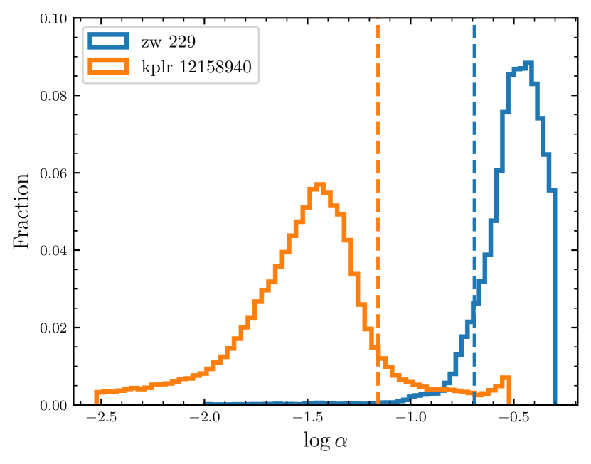
Our results demonstrate that, for light curves with sufficient quality (especially on long timescales), we can in principle infer the value of $\alpha$ by fitting the AGN UV/optical light curves. The fits to the three Kepler AGNs already suggest that different AGNs have different $\alpha$ values. The required $\alpha$ is not entirely consistent with the values derived from some recent radiation MHD shearing box simulations of accretion disks where $\alpha$ converges around $0.01$ (Blaes, 2014). A similar discrepancy is also found when analyzing the observations of outbursts of dwarf nova or soft X-ray transients (King et al., 2007). Some possible explanation involve the large-scale poloidal magnetic field (as illustrated in Figure 1, the large-scale magnetic field is also required in our CHAR model) because $\alpha$ positively correlates with the initial field strength (see Figure 6 of Hawley et al., 1995) or the kinetic effect of MRI turbulence (e.g., Kunz et al., 2016); a detail discussion of additional possibilities has been made by King et al. (2007).

4.2 NGC 5548

Our CHAR model also has the potential to self-consistently account for other observational characteristics of AGN UV/optical variability, e.g., the multi-wavelength variability of the best-studied reverberation-mapped AGN, NGC 5548. To apply our CHAR model to NGC 5548, we fix the mass of the central SMBH to be $M_{\mathrm{BH}}=5\times 10^{7}\ M_{\odot}$ and choose $\dot{M}$ such that the model luminosity at $5100$ Å is consistent with the observed one (Fausnaugh et al., 2016); $\delta_{\mathrm{mc}}$ is adjusted to ensure that the structure function at $10$ days of the model light curve at $B$-band matches the observed one. The remaining parameter is $\alpha=0.2$. We then run simulations to generate eighteen-band model light curves (i.e., all the eighteen UV/optical bands listed in table 5 of Fausnaugh et al. 2016; we do not consider X-ray observations because X-ray emission is not produced by the accretion disk but by the hot corona) following the methodology mentioned above. During the simulations, the time-sampling issues and the measurement errors are also considered, i.e., the model light curves share the same cadence and measurement noise as the observations of NGC 5548 (Fausnaugh et al., 2016).

Figure 21: The SFs of NGC 5548 for various wavelengths (annotated top). The stars and the purple curve represent the observed and the model SFs, respectively; the shaded regions indicate the $1\sigma$ uncertainties. The SFs for all eighteen bands are available online.

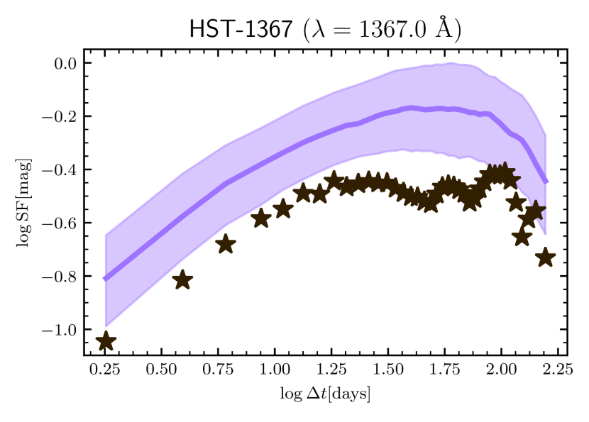
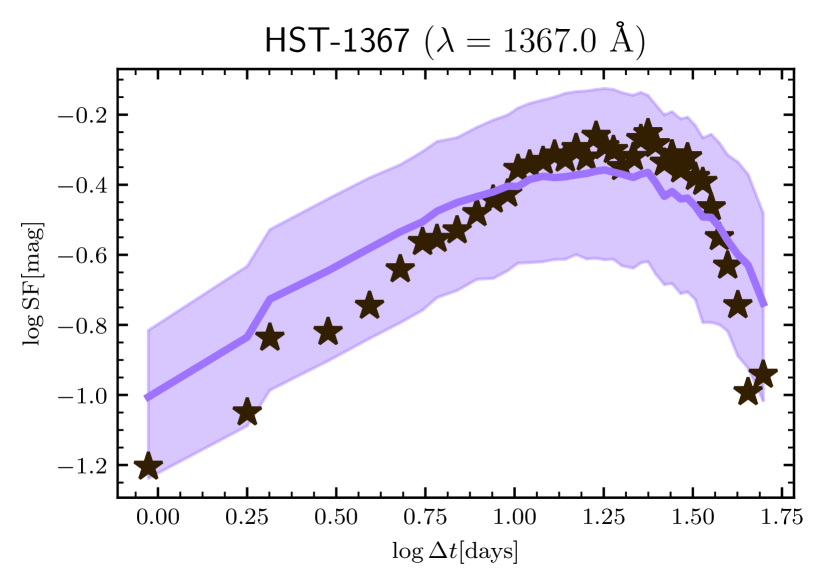
For each band, we first compare the model SF with the observed one (see Figure 21 for the SDSS $i$-band; the complete figure set for all bands is available online). Overall, our model can account for the observed SFs of the multi-band light curves of NGC 5548 on timescales $\lesssim 20$ days. On timescales of $20$–$50$ days, our CHAR model over-predicts the observed variability. This deviation might have something to do with the anomalous state (Goad et al., 2016) in NGC 5548; in the anomalous state, the ionizing continuum is preferentially suppressed due to, e.g., the intrinsic change of the corona/disk structure (Mathur et al., 2017; Sun et al., 2018b) or external variations in line-of-sight obscuration (Dehghanian et al., 2019; Kriss et al., 2019). Indeed, if we split the full multi-wavelength light curves of NGC 5548 into two segments at $\mathrm{HJD}-2450000<6747$, the first portions are more variable than the second ones, especially on timescales longer than $10$ days (see Figure 5 of Sun et al., 2018b). We then re-apply our CHAR model to the first segment of each band of the NGC 5548 light curve following the same methodology. The resulting SFs are shown in Figure 22. Our CHAR model can now also explain the observed SFs of NGC 5548 on timescales $\gtrsim 20$ days. Therefore, our results indicate that the magnetic fluctuations in the corona might also change as NGC 5548 entered into the anomalous state.

Figure 22: The SFs of NGC 5548 for various wavelengths (annotated top). Unlike Figure 21, only the first portions (i.e., data points with $\mathrm{HJD}-2450000<6747$) of the light curves are considered here. The stars and the purple curve represent the observed and the model SFs, respectively; the shaded regions indicate the $1\sigma$ uncertainties. The SFs for all eighteen bands are available online.

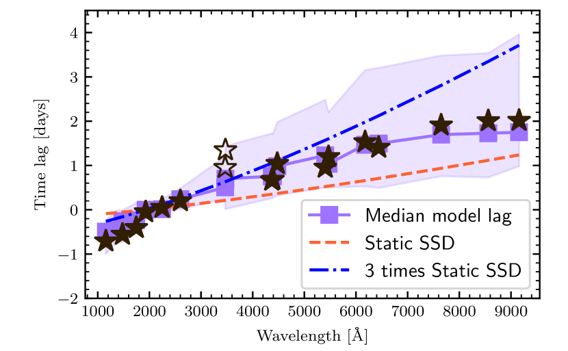
We then use PYCCF (Sun et al., 2018a), a python version of the interpolation cross-correlation function code (Peterson et al., 1998), to determine the inter-band time lags for the model light curves; the reference band is chosen to be the Swift UVW2 band (Edelson et al., 2019). We also use our code to re-estimate the observed time lags for the sake of self-consistency. We limit our analyses to the first segments of the multi-wavelength light curves of NGC 5548. Our CHAR model can explain the observed inter-band time lags which are larger than the expectations of the lamppost model (see Figure 23). This is because, unlike the lamppost model, the disk temperature cannot fully respond to the variations of $Q^{+}_{\mathrm{heat}}$ unless a thermal timescale has passed. That is, the inter-band time lags are superpositions of the magnetic fluctuation travel (the speed is assumed to be the speed of light) timescales and the response timescales (see Section 3.2.3).

Figure 23: The inter-band time lags of NGC 5548. Only the first portions (i.e., data points with $\mathrm{HJD}-2450000<6747$) of the light curves are considered here. The stars and the squares represent the observed and the median model time lags, respectively. The open stars correspond to the time lags of the $U$ and $u$ bands which are likely to be affected by broad-line region emission. The purple shaded regions indicate the $1\sigma$ uncertainties of the model time lags. The red dashed curve shows the expected time lags of the static thin disk model; the blue dashed-dot curve indicates the expected time lags if we increase the static thin disk sizes by a factor of three. Note that our modeling approach for NGC 5548 includes the same time-sampling pattern and photometric errors as the inter-band time lags estimated from the real light curves.

5 Discussion

5.1 Physical Mechanisms

Considering the large optical depth from the surface to the mid-plane, external illumination (e.g., X-ray or UV emission) should be absorbed within a thin surface of the accretion disk. If so, the timescale for such a thin surface to adjust its structure and the absorbed energy to be reprocessed as UV/optical emission is rather short (it can be less than one hour; see, e.g., Collin-Souffrin, 1991; Czerny, 2006); that is, Eq. 1 seems to be valid. However, as we discussed in Section 1, this simple and interesting model fails to explain many observational facts of AGN UV/optical variability (see also Edelson et al., 2019).

To overcome these problems, we propose that the corona and the accretion disk are tightly coupled by magnetic fields. Turbulent magnetic fields are well expected in an accretion disk since the MRI is responsible for removing angular momentum, releasing the gravitational energy and heating the gas in the accretion disk (Balbus & Hawley, 1998). The interior magnetic fields might rise to the low-density surface owing to, e.g., magnetic buoyancy (Parker, 1966) and can be effectively amplified to form large-scale poloidal magnetic fields (Rothstein & Lovelace, 2008). In the vertical regions that are well above the accretion disk, the gas is highly magnetized; the puffed-up magnetic field might reconnect, dissipate its energy, and heat the ambient low-density plasma (e.g., Di Matteo, 1998; Liu et al., 2002). If the dissipated energy is mainly converted into the internal energy of protons, and protons and electrons are largely decoupled (given the low-density nature, Coulomb coupling is inefficient; see e.g., Di Matteo 1998; Różańska & Czerny 2000), the plasma will be radiatively inefficient (which is similar to an advection-dominated accretion flow; see Yuan & Narayan, 2014). This hot and radiatively inefficient plasma might be responsible for the so-called “X-ray corona”. The magnetic power might also launch a relativistic jet from the coronal plasma (i.e., the corona might serve as the jet base; Markoff et al., 2005). In addition, the SMBHs might be supplied by the ambient hot gas (e.g., from stellar winds) and the accretion flow around the Bondi radius can be geometrically thick; an underlying thin and cold disk only forms at much smaller radii; then, the “X-ray corona” might be the innermost regions of this thick disk (Liu et al., 2015). Unlike the underlying cold thin disk (Shakura & Sunyaev, 1973), the corona should have a large inflow velocity (Liu et al., 2015; Jiang et al., 2019) since the plasma is hot and the angular-momentum transfer due to the MRI should be efficient. Therefore, the anchored magnetic field in the corona can be “dragged” into the innermost regions. The same magnetic field that penetrates the interior of the cold accretion disk remains in its original radial location as the inflow velocity of the cold disk is small. Therefore, a magnetic coupling between the compact corona and the outer cold accretion disk might exist (see Figure 1).

As the magnetic field of the corona fluctuates (due to, e.g., magnetic reconnection), the disk turbulent magnetic field also changes accordingly after a time delay which accounts for the propagation of MHD waves from the corona to the disk; the time delay $t_{\mathrm{delay}}$ is $R_{X}/c_{\mathrm{avf}}$, where $R_{X}$ and $c_{\mathrm{avf}}$ are the distance between the corona and the disk and the Alfvén velocity, respectively. The coherently variable disk turbulent magnetic power (i.e., the fluctuations of disk turbulent magnetic field at different radii are correlated) dissipates and changes the heating rate in the disk. As a result, the interior structure of the accretion disk changes in response to the variable disk heating rate. The timescale for the disk temperature to adjust to the variable disk heating rate is the thermal timescale. On timescales significantly longer than the thermal timescale, the disk temperature and the disk heating rate vary similarly; but on timescales shorter than the thermal timescale, the disk response time is important and the disk variability is less than the fluctuation in the heating rate. This naturally leads to less variability on short timescales and more variability on long timescales, explaining why the thermal timescale is a good fit to the “break” timescale between the two variability regimes (e.g., Kelly et al., 2009; Sun et al., 2015, 2018d).

5.2 The Correlation Between X-ray and UV/optical Variability

In this work, we assume that the disk-temperature variations are induced by corona magnetic fluctuations; the same magnetic fluctuations can also drive X-ray variability. Therefore, one might expect a tight correlation between UV/optical and X-ray emission. However, the relationship between $Q_{\mathrm{mc}}^{+}$ and X-ray emission can be complicated due to the important advective cooling and the fluctuations of the corona surface density (see also Section 3.2.3). A detailed investigation of this topic is needed to understand the relation between X-ray and UV/optical stochastic variations; however, this is beyond the scope of this work.

5.3 Relationship To Other Models

Alternative models have been proposed to explain AGN UV/optical light curves. One of the most popular models is the X-ray reprocessing model (e.g., Krolik et al., 1991). In this model, the highly variable X-ray emission (which is presumably produced in the hot corona) can illuminate the underlying cold accretion disk; a significant fraction of the illuminating X-ray photons are thermalized in the disk surface. The absorbed X-ray emission is reprocessed as the UV/optical emission which might be responsible for the observed AGN UV/optical light curves. However, this scenario is challenged by many observations (Uttley et al. 2003; Sun et al. 2014; Fausnaugh et al. 2016; Cai et al. 2018; Kang et al. 2018; Zhu et al. 2018; Edelson et al. 2019; see also Section 1).

Variations of accretion rate at each radius can also induce AGN luminosity fluctuations. In fact, Lyubarskii (1997) demonstrated that, if the accretion rate at each radius varies independently, the PSD of the AGN bolometric luminosity is $\propto 1/f$. However, the required timescale for the accretion rate to vary is the viscous timescale, which should be around hundreds of years for the UV/optical emission regions of a typical AGN. Therefore, this model cannot explain the observed UV/optical variability. Instead, it might be able to explain the short-timescale (i.e., hours to years) magnetic energy fluctuations in the innermost regions or the compact corona where the corresponding viscous timescale can be less than days.

Another popular model is the strongly inhomogeneous disk model (Dexter & Agol, 2011; Cai et al., 2016). While this model has the potential to explain the microlensing observations (Morgan et al., 2010), the timescale-dependent AGN color variability (Sun et al., 2014), and many other observational characteristics, the temperature fluctuations in this model are “assumed” to be a DRW process. Meanwhile, this model fails to explain the inter-band cross correlations since the temperature fluctuations at different radii vary independently. Cai et al. (2018) upgraded the strongly inhomogeneous disk model by adding a global common temperature fluctuation and found that this new model has the potential to yield the observed inter-band UV/optical time lags (Fausnaugh et al., 2016; Edelson et al., 2019). However, temperature fluctuations in Cai et al. (2018) are still assumed to be a DRW process.

All in all, a model to account for the AGN UV/optical variability has long been lacking until our work where we propose a simple way to determine the temperature fluctuations in the accretion disk and explain AGN UV/optical light curves.

5.4 LSST Forecasts

It has been shown in previous sections that our CHAR model can well explain the multi-wavelength variability of the AGNs that have the best-quality observations available . The variability properties depend critically on our CHAR model’s free parameters, namely, $M_{\mathrm{BH}}$, $\alpha$, $\dot{M}$ (or $\dot{m}$) and $\delta_{\mathrm{mc}}$. It is then possible to constrain these parameters by adopting our CHAR model to fit future LSST light curves. To illustrate this idea, we consider five AGNs with five different choices of $M_{\mathrm{BH}}$, $\dot{M}$, and $\alpha$, i.e., $M_{7}=1$, $\dot{M}_{24}=1.3$, and $\alpha=0.2$ (hereafter case I); $M_{7}=5$, $\dot{M}_{24}=1.3$, and $\alpha=0.2$ (hereafter case II); $M_{7}=5$, $\dot{M}_{24}=0.08$, and $\alpha=0.05$ (hereafter case III); $M_{7}=1$, $\dot{M}_{24}=6.5$, and $\alpha=0.2$ (hereafter case IV); $M_{7}=5$, $\dot{M}_{24}=1.3$, and $\alpha=0.01$ (hereafter case V). Note that $M_{7}=M_{\mathrm{BH}}/(10^{7}M_{\odot})$ and $\dot{M}_{24}=\dot{M}/(10^{24}\ \mathrm{g\ s^{-1}})$.

For each case, we use our CHAR model to simulate the light curves of the observed-frame $3500$ Å and $8500$ Å (which correspond to the central wavelengths of the $u$ and $z$ bands of the LSST filters, respectively) emission; the duration of every light curve is $10$ years (in the observed frame); the photometric noise is assumed to be $0.01$ mag and the cadence of the simulations is (observed-frame) $3$-day which is motivated by the LSST surveys of the deep-drilling fields (Brandt et al., 2018; Scolnic et al., 2018). For each case, we repeat the simulation $512$ times to account for statistical fluctuations due to photometric noise, limited cadence, and duration. For each case, $\delta_{\mathrm{mc}}$ is chosen to ensure that the SF of the $3500$ Å emission at $50$ days is the same (i.e., $\cong 0.03$ mag).

The SFs of the observed-frame $3500$ Å and $8500$ Å emission and their ratios are calculated. The ratios are similar to the color variability in Section 3.2.5. That is, a bluer-when-brighter behavior is expected if the ratio is smaller than unity.

Figure 24: The predicted statistical properties of AGN UV/optical light curves as a function of $M_{7}$, $\dot{M}_{24}$ and $\alpha$, where $M_{7}=M_{\mathrm{BH}}/(10^{7}M_{\odot})$ and $\dot{M}_{24}=\dot{M}/(10^{24}\ \mathrm{g\ s^{-1}})$. The cadence is assumed to be 3 days which is motivated by the LSST surveys in the deep-drilling fields. Left: the SFs of the observed-frame $3500$ Å emission (which corresponds to the LSST $u$ band). Middle: the ratios of the SFs of the $8500$ Å emission (which corresponds to the LSST $z$ band) to those of the observed-frame $3500$ Å emission (the ratios are similar to the color variability in Section 3.2.5, i.e., a bluer-when-brighter behavior is expected if the ratio is smaller than unity). Right: the corresponding spectral energy distributions. The shaded regions represent the $1\sigma$ uncertainties (the uncertainties of the SFs of cases II and III are not shown for the purpose of clarity). By simultaneously considering all the three properties, we can distinguish AGNs with different physical parameters and thereby constrain $M_{\mathrm{BH}}$, $\dot{M}$, and $\alpha$ given LSST datasets. The redshifts of these mock AGNs are fixed to $z=0.017175$ (i.e., the same as that of NGC 5548).

Figure 25: Same as Figure 24, but for mock AGNs at $z=1$.

The SFs of the $3500$ Å emission, the ratios of the SFs of the $8500$ Å emission to those of the $3500$ Å emission, and the expected SEDs are shown in Figure 24 for AGNs at $z=0.017175$ (i.e., the same as that of NGC 5548). The results for the same AGNs at $z=1$ are presented in Figure 25. The differences in the SFs are evident beyond the measurement noise if the corresponding $\tau_{\mathrm{TH}}$ ($\propto\dot{M}^{0.5}\alpha^{-1}$; see Eq. 12) values are significantly different (i.e., comparing case I or II with case IV or V). While the SFs of cases A, B and C (they have similar $\tau_{\mathrm{TH}}$) are indistinguishable within measurement noise, their color variability is statistically different. Therefore, it is promising to infer $\dot{M}$ and $\alpha$ by considering the LSST light curves of thousands of type I AGNs in the LSST deep-drilling fields. The SEDs are sensitive to both $\dot{M}$ and $M_{\mathrm{BH}}$. Hence, as long as $\dot{M}$ is determined, we can also infer $M_{\mathrm{BH}}$ from the LSST data. Note that many of the brightest AGNs in the LSST deep-drilling fields will also have independent $M_{\mathrm{BH}}$ measurements from the reverberation-mapping campaigns, e.g., the SDSS-V Black Hole Mapper (Kollmeier et al., 2017) and 4MOST/TiDES (Swann et al., 2019). Then, we can use the two independent $M_{\mathrm{BH}}$ measurements to perform a cross-validation study to improve the accuracy of $M_{\mathrm{BH}}$. Moreover, the radiative efficiency $\eta\equiv L_{\mathrm{bol}}/(\dot{M}c^{2})$ can be calculated. For radiatively efficient accretion disks, $\eta$ should be determined by the innermost stable circular orbit (ISCO) radius $R_{\mathrm{ISCO}}$ and magnetic stress at this radius (Agol & Krolik, 2000); $R_{\mathrm{ISCO}}$ depends on the SMBH spin $a^{*}$. Therefore, we can use the measured $\eta$ to deliver some insights on $a^{*}$ and/or magnetic stress at $R_{\mathrm{ISCO}}$.

6 Summary

We propose a new model, Corona-Heated Accretion-disk Reprocessing (a.k.a., CHAR), to explain AGN UV/optical variability. In contrast to the simplest X-ray reprocessing model, we argue that, as the corona induces fluctuations in the heating rate, the temperature of the interior of an AGN accretion disk also changes. We assume that the AGN accretion disk can re-establish vertical hydrostatic equilibrium, and the variability of $Q_{\mathrm{mc}}^{+}$ can be described by a red-noise process. Then, the temperature fluctuations can be determined by considering the vertically integrated thermal-energy conservation law (see Eq. 9 and Section 2).

We solve Eq. 9 to obtain the temperature fluctuations and luminosity variability. We find that the fluctuations of the inner and surface temperature and luminosity differ from that of $Q_{\mathrm{mc}}^{+}$ in many aspects. Our main results can be summarized as follows.

1. The fluctuations of the inner and surface temperature and luminosity contain less high-frequency components than that of $Q_{\mathrm{mc}}^{+}$ (see Figures 2, 3 and 4; Section 3.2.1).

2. According to our CHAR model, on timescales of $10^{2}$—$10^{3}$ days, AGN UV/optical luminosity variability can be well fitted by the DRW process; on shorter/longer timescales, the DRW process under-predicts/over-predicts AGN UV/optical luminosity variability (see Figure 4).

3. The PSD and SF of AGN UV/optical luminosity variability have a characteristic timescale, i.e., the thermal timescale $\tau_{\mathrm{TH}}$ (see Eq. 12; Section 2.2).

4. The PSD and SF depend mostly on AGN luminosity or $\dot{M}$ (see Figure 15; Section 3.3); their dependences on $M_{\mathrm{BH}}$ or $\dot{m}$ are weak.

5. AGN UV/optical luminosity variability decreases with increasing wavelength; the difference is more evident on short timescales (see Figure 5).

6. Our CHAR model predicts a bluer-when-brighter behavior (see Figure 10); the bluer-when-brighter behavior is more evident on short timescales than on long timescales (see Figure 11).

7. AGN timescale-dependent color variability (bluer-when-brighter) correlates with $\dot{m}$ and $L_{\mathrm{bol}}$; its dependence on $M_{\mathrm{BH}}$ is complex (see Figures 10 and 11; Section 3.3.2).

8. Unlike the X-ray reprocessing model, the inter-band time lags of our CHAR model increase with increasing timescales (see Figure 7; Section 3.2.3). For an AGN with $M_{\mathrm{BH}}=10^{8}\ M_{\odot}$ and $L=0.1L_{\mathrm{Edd}}$, on timescales of $\sim 10^{2}$ days, the inter-band time lags between UV and optical bands can be $\sim 3$ times larger than the expectations of the static SSD model.

9. Our CHAR model might also be able to explain AGN microlensing observations (see Figure 9; Section 3.2.4).

10. Our CHAR model can successfully explain the high-quality Kepler AGN light curves (see Figure 18; Section 4.1); the dimensionless viscosity, one of the basic parameters in the black hole accretion theory, which cannot be determined by fitting AGN SEDs, is constrained to be $0.01$—$0.2$ by our CHAR model.

11. Our CHAR model can also account for the lager-than-expected time lags in NGC 5548 (see Figure 23). With the same parameters, our CHAR model can simultaneously fit the SFs of the eighteen light curves of NGC 5548 (see Figure 22; Section 4.2).

12. We demonstrate that $M_{\mathrm{BH}}$, $\dot{M}$, and $\alpha$ can be constrained by applying our CHAR model to fit AGN multi-band light curves from LSST time-domain surveys (see Figures 24 and 25; Section 5.4).

Therefore, our CHAR model has the potential to explain many observational facts about AGN UV/optical variability.

If our CHAR model is correct, the time lag between optical and the ionizing continuum emission can be significant on long timescales (see Figure 7; Section 3.2.3). Most RM campaigns usually measure the time lag between the BEL and the nearby optical emission. Therefore, the distance of BLR to the central SMBH can be significantly under-estimated for a long-term (i.e., the nearby continuum light curve contains long-term variability) RM campaign. This bias can be corrected by performing long-term detrending to the RM light curves.

Our work can be advanced in some theoretical aspects. For instance, disk winds can be strong and modify the structure of the accretion disk (Sun et al., 2019) and the disk emission may not be a perfect black body (Hall et al., 2018). We also ignore the UV/optical variability due to X-ray reprocessing of a static SSD or diffuse BLR clouds (e.g., Cackett et al., 2018; Sun et al., 2018b). It would be interesting to revise our CHAR model to include these physical processes. In addition, our analysis cannot be applied to timescales comparable to the viscous timescales unless accretion-rate fluctuations (which can be significant due to, e.g., radiation-pressure instabilities) are properly modeled; such accretion-rate fluctuations have been proposed to explain the intermittent activity of compact GPS radio sources (Czerny et al., 2009).

In future works, we will test our model with additional observations, e.g., the inter-band cross correlations and time lags of other AGNs (Edelson et al., 2019), microlensing observations (Morgan et al., 2010), and other more sparse AGN light curves (Kelly et al., 2009; MacLeod et al., 2010). It could also be interesting to apply our CHAR model to fit the extremely short-timescale ($\gtrsim 100$ Hz) variability observed in black hole X-ray binaries.

References

- Abramowicz et al. (1988) Abramowicz, M. A., Czerny, B., Lasota, J. P., & Szuszkiewicz, E. 1988, ApJ, 332, 646
- Agol & Krolik (2000) Agol, E., & Krolik, J. H. 2000, ApJ, 528, 161
- Ai et al. (2010) Ai, Y. L., Yuan, W., Zhou, H. Y., et al. 2010, ApJ, 716, L31
- Astropy Collaboration et al. (2018) Astropy Collaboration, Price-Whelan, A. M., Sipőcz, B. M., et al. 2018, AJ, 156, 123
- Balbus & Hawley (1998) Balbus, S. A., & Hawley, J. F. 1998, Reviews of Modern Physics, 70, 1
- Barth et al. (2011) Barth, A. J., Nguyen, M. L., Malkan, M. A., et al. 2011, ApJ, 732, 121
- Bentz et al. (2009) Bentz, M. C., Walsh, J. L., Barth, A. J., et al. 2009, ApJ, 705, 199
- Blaes (2014) Blaes, O. 2014, Space Sci. Rev., 183, 21
- Blandford & McKee (1982) Blandford, R. D., & McKee, C. F. 1982, ApJ, 255, 419
- Borucki et al. (2010) Borucki, W. J., Koch, D., Basri, G., et al. 2010, Science, 327, 977
- Brandt et al. (2018) Brandt, W. N., Ni, Q., Yang, G., et al. 2018, arXiv:1811.06542
- Cackett et al. (2018) Cackett, E. M., Chiang, C.-Y., McHardy, I., et al. 2018, ApJ, 857, 53
- Cackett et al. (2007) Cackett, E. M., Horne, K., & Winkler, H. 2007, MNRAS, 380, 669
- Cai et al. (2016) Cai, Z.-Y., Wang, J.-X., Gu, W.-M., et al. 2016, ApJ, 826, 7
- Cai et al. (2018) Cai, Z.-Y., Wang, J.-X., Zhu, F.-F., et al. 2018, ApJ, 855, 117
- Capellupo et al. (2015) Capellupo, D. M., Netzer, H., Lira, P., et al. 2015, MNRAS, 446, 3427
- Chen & Wang (2015) Chen, X.-Y., & Wang, J.-X. 2015, ApJ, 805, 80
- Ciesielski et al. (2012) Ciesielski, A., Wielgus, M., Kluźniak, W., et al. 2012, A&A, 538, A148
- Clavel et al. (1992) Clavel, J., Nandra, K., Makino, F., et al. 1992, ApJ, 393, 113
- Collin-Souffrin (1991) Collin-Souffrin, S. 1991, A&A, 249, 344
- Cornachione et al. (2019) Cornachione, M. A., Morgan, C. W., Millon, M., et al. 2019, arXiv e-prints, arXiv:1911.06218
- Czerny (2006) Czerny, B. 2006, AGN Variability from X-Rays to Radio Waves, 360, 265
- Czerny & Elvis (1987) Czerny, B., & Elvis, M. 1987, ApJ, 321, 305
- Czerny et al. (2004) Czerny, B., Różańska, A., Dovčiak, M., Karas, V., & Dumont, A.-M. 2004, A&A, 420, 1
- Czerny et al. (2009) Czerny, B., Siemiginowska, A., Janiuk, A., Nikiel-Wroczyński, B., & Stawarz, Ł. 2009, ApJ, 698, 840
- Dehghanian et al. (2019) Dehghanian, M., Ferland, G. J., Kriss, G. A., et al. 2019, ApJ, 877, 119
- Dexter & Agol (2011) Dexter, J., & Agol, E. 2011, ApJ, 727, L24
- Dexter et al. (2019) Dexter, J., Xin, S., Shen, Y., et al. 2019, ApJ, 885, 44
- Di Matteo (1998) Di Matteo, T. 1998, MNRAS, 299, L15
- Du et al. (2016) Du, P., Lu, K.-X., Zhang, Z.-X., et al. 2016, ApJ, 825, 126
- Dubus et al. (2001) Dubus, G., Hameury, J.-M., & Lasota, J.-P. 2001, A&A, 373, 251
- Edelson et al. (2019) Edelson, R., Gelbord, J., Cackett, E., et al. 2019, ApJ, 870, 123
- Emmanoulopoulos et al. (2010) Emmanoulopoulos, D., McHardy, I. M., & Uttley, P. 2010, MNRAS, 404, 931
- Fausnaugh et al. (2016) Fausnaugh, M. M., Denney, K. D., Barth, A. J., et al. 2016, ApJ, 821, 56
- Foreman-Mackey et al. (2013) Foreman-Mackey, D., Hogg, D. W., Lang, D., et al. 2013, PASP, 125, 306
- Gardner & Done (2017) Gardner, E., & Done, C. 2017, MNRAS, 470, 3591
- Goad et al. (2016) Goad, M. R., Korista, K. T., De Rosa, G., et al. 2016, ApJ, 824, 11
- Grier et al. (2019) Grier, C. J., Shen, Y., Horne, K., et al. 2019, arXiv:1904.03199
- Grier et al. (2017) Grier, C. J., Trump, J. R., Shen, Y., et al. 2017, ApJ, 851, 21
- Guo et al. (2017) Guo, H., Wang, J., Cai, Z., & Sun, M. 2017, ApJ, 847, 132
- Haardt & Maraschi (1991) Haardt, F., & Maraschi, L. 1991, ApJ, 380, L51
- Hall et al. (2018) Hall, P. B., Sarrouh, G. T., & Horne, K. 2018, ApJ, 854, 93
- Hawley et al. (1995) Hawley, J. F., Gammie, C. F., & Balbus, S. A. 1995, ApJ, 440, 742
- Hirose et al. (2009) Hirose, S., Krolik, J. H., & Blaes, O. 2009, ApJ, 691, 16
- Homayouni et al. (2019) Homayouni, Y., Trump, J. R., Grier, C. J., et al. 2019, ApJ, 880, 126
- Hunter (2007) Hunter, J. D. 2007, Computing in Science and Engineering, 9, 90
- Ivezić et al. (2019) Ivezić, Ž., Kahn, S. M., Tyson, J. A., et al. 2019, ApJ, 873, 111
- Jiang et al. (2019) Jiang, Y.-F., Blaes, O., Stone, J., & Davis, S.W. 2019, ApJ, 885, 144
- Jiang et al. (2017) Jiang, Y.-F., Green, P. J., Greene, J. E., et al. 2017, ApJ, 836, 186
- Jiang et al. (2013) Jiang, Y.-F., Stone, J. M., & Davis, S. W. 2013, ApJ, 778, 65
- Just et al. (2007) Just, D. W., Brandt, W. N., Shemmer, O., et al. 2007, ApJ, 665, 1004
- Kang et al. (2018) Kang, W.-Y., Wang, J.-X., Cai, Z.-Y., et al. 2018, ApJ, 868, 58
- Kasliwal et al. (2015) Kasliwal, V. P., Vogeley, M. S., & Richards, G. T. 2015, MNRAS, 451, 4328
- Kato et al. (2008) Kato, S., Fukue, J., & Mineshige, S. 2008, Black-Hole Accretion Disks: Towards a New Paradigm (Kyoto: Kyoto University Press)
- Kelly et al. (2009) Kelly, B. C., Bechtold, J., & Siemiginowska, A. 2009, ApJ, 698, 895
- Kelly et al. (2014) Kelly, B. C., Becker, A. C., Sobolewska, M., Siemiginowska, A., & Uttley, P. 2014, ApJ, 788, 33
- Kinemuchi et al. (2012) Kinemuchi, K., Barclay, T., Fanelli, M., et al. 2012, PASP, 124, 963
- King et al. (2004) King, A. R., Pringle, J. E., West, R. G., & Livio, M. 2004, MNRAS, 348, 111
- King et al. (2007) King, A. R., Pringle, J. E., & Livio, M. 2007, MNRAS, 376, 1740
- Kriss et al. (2019) Kriss, G. A., De Rosa, G., Ely, J., et al. 2019, ApJ, 881, 153
- Kokubo (2015) Kokubo, M. 2015, MNRAS, 449, 94
- Kokubo (2018) Kokubo, M. 2018, PASJ, 70, 97
- Kollmeier et al. (2017) Kollmeier, J. A., Zasowski, G., Rix, H.-W., et al. 2017, arXiv e-prints, arXiv:1711.03234
- Kozłowski (2017) Kozłowski, S. 2017, A&A, 597, A128
- Krolik et al. (1991) Krolik, J. H., Horne, K., Kallman, T. R., et al. 1991, ApJ, 371, 541
- Kunz et al. (2016) Kunz, M. W., Stone, J. M., & Quataert, E. 2016, Phys. Rev. Lett., 117, 235101
- Laor & Davis (2014) Laor, A., & Davis, S. W. 2014, MNRAS, 438, 3024
- Lasota (2001) Lasota, J.-P. 2001, New A Rev., 45, 449
- Lawrence (2018) Lawrence, A. 2018, Nature Astronomy, 2, 102
- Li & Cao (2008) Li, S.-L., & Cao, X. 2008, MNRAS, 387, L41
- Li et al. (2018) Li, Z., McGreer, I. D., Wu, X.-B., Fan, X., & Yang, Q. 2018, ApJ, 861, 6
- Li et al. (2019) Li, Y.-P., Yuan, F., & Dai, X. 2019, MNRAS, 483, 2275
- Lin et al. (2011) Lin, D.-B., Gu, W.-M., & Lu, J.-F. 2011, MNRAS, 415, 2319
- Lin et al. (2012) Lin, D.-B., Gu, W.-M., Liu, T., Sun, M.-Y., & Lu, J.-F. 2012, ApJ, 761, 29
- Lin et al. (2016) Lin, D.-B., Lu, Z.-J., Mu, H.-J., et al. 2016, MNRAS, 463, 245
- Liu et al. (2016) Liu, H., Li, S.-L., Gu, M., & Guo, H. 2016, MNRAS, 462, L56
- Liu et al. (2002) Liu, B. F., Mineshige, S., & Shibata, K. 2002, ApJ, 572, L173
- Liu et al. (2007) Liu, B. F., Taam, R. E., Meyer-Hofmeister, E., & Meyer, F. 2007, ApJ, 671, 695
- Liu et al. (2015) Liu, B. F., Taam, R. E., Qiao, E., et al. 2015, ApJ, 806, 223
- Lyubarskii (1997) Lyubarskii, Y. E. 1997, MNRAS, 292, 679
- MacLeod et al. (2010) MacLeod, C. L., Ivezić, Ž., Kochanek, C. S., et al. 2010, ApJ, 721, 1014
- MacLeod et al. (2012) MacLeod, C. L., Ivezić, Ž., Sesar, B., et al. 2012, ApJ, 753, 106
- MacLeod et al. (2016) MacLeod, C. L., Ross, N. P., Lawrence, A., et al. 2016, MNRAS, 457, 389
- Markoff et al. (2005) Markoff, S., Nowak, M. A., & Wilms, J. 2005, ApJ, 635, 1203
- Marshall et al. (1997) Marshall, H. L., Carone, T. E., Peterson, B. M., et al. 1997, ApJ, 479, 222
- Mathur et al. (2017) Mathur, S., Gupta, A., Page, K., et al. 2017, ApJ, 846, 55
- McHardy et al. (2018) McHardy, I. M., Connolly, S. D., Horne, K., et al. 2018, MNRAS, 480, 2881
- Morgan et al. (2010) Morgan, C. W., Kochanek, C. S., Morgan, N. D., et al. 2010, ApJ, 712, 1129
- Morganson et al. (2014) Morganson, E., Burgett, W. S., Chambers, K. C., et al. 2014, ApJ, 784, 92
- Mudd et al. (2018) Mudd, D., Martini, P., Zu, Y., et al. 2018, ApJ, 862, 123
- Mushotzky et al. (2011) Mushotzky, R. F., Edelson, R., Baumgartner, W., & Gandhi, P. 2011, ApJ, 743, L12
- Noble & Krolik (2009) Noble, S. C., & Krolik, J. H. 2009, ApJ, 703, 964
- Parker (1966) Parker, E. N. 1966, ApJ, 145, 811
- Peterson (2014) Peterson, B. M. 2014, Space Sci. Rev., 183, 253
- Peterson et al. (1998) Peterson, B. M., Wanders, I., Horne, K., et al. 1998, PASP, 110, 660
- Rothstein & Lovelace (2008) Rothstein, D. M., & Lovelace, R. V. E. 2008, ApJ, 677, 1221
- Różańska & Czerny (2000) Różańska, A., & Czerny, B. 2000, A&A, 360, 1170
- Ruan et al. (2014) Ruan, J. J., Anderson, S. F., Dexter, J., & Agol, E. 2014, ApJ, 783, 105
- Sánchez-Sáez et al. (2018) Sánchez-Sáez, P., Lira, P., Mejía-Restrepo, J., et al. 2018, ApJ, 864, 87
- Scolnic et al. (2018) Scolnic, D. M., Lochner, M., Gris, P., et al. 2018, arXiv e-prints, arXiv:1812.00516
- Sergeev et al. (2005) Sergeev, S. G., Doroshenko, V. T., Golubinskiy, Y. V., Merkulova, N. I., & Sergeeva, E. A. 2005, ApJ, 622, 129
- Shakura & Sunyaev (1973) Shakura, N. I., & Sunyaev, R. A. 1973, A&A, 24, 337
- Shen (2013) Shen, Y. 2013, Bulletin of the Astronomical Society of India, 41, 61
- Simm et al. (2016) Simm, T., Salvato, M., Saglia, R., et al. 2016, A&A, 585, A129
- Slone & Netzer (2012) Slone, O., & Netzer, H. 2012, MNRAS, 426, 656
- Smith et al. (2018a) Smith, K. L., Mushotzky, R. F., Boyd, P. T., et al. 2018a, ApJ, 857, 141
- Smith et al. (2018b) Smith, K. L., Mushotzky, R. F., Boyd, P. T., et al. 2018b, ApJ, 860, L10
- Starkey et al. (2017) Starkey, D., Horne, K., Fausnaugh, M. M., et al. 2017, ApJ, 835, 65
- Sun et al. (2015) Sun, M., Trump, J. R., Shen, Y., et al. 2015, ApJ, 811, 42
- Sun et al. (2018a) Sun, M., Grier, C. J., Peterson, B. M. 2018a, PYCCF, Astrophysics Source Code Library, record ascl:1805.032
- Sun et al. (2018b) Sun, M., Xue, Y., Cai, Z., & Guo, H. 2018a, ApJ, 857, 86
- Sun et al. (2018c) Sun, M., Xue, Y., Richards, G. T., et al. 2018b, ApJ, 854, 128
- Sun et al. (2018d) Sun, M., Xue, Y., Wang, J., Cai, Z., & Guo, H. 2018c, ApJ, 866, 74
- Sun et al. (2019) Sun, M., Xue, Y., Trump, J. R., & Gu, W.-M. 2019, MNRAS, 482, 2788
- Sun et al. (2014) Sun, Y.-H., Wang, J.-X., Chen, X.-Y., & Zheng, Z.-Y. 2014, ApJ, 792, 54
- Swann et al. (2019) Swann, E., Sullivan, M., Carrick, J., et al. 2019, The Messenger, 175, 58
- Tie & Kochanek (2018) Tie, S. S., & Kochanek, C. S. 2018, MNRAS, 473, 80
- Trump et al. (2011) Trump, J. R., Impey, C. D., Kelly, B. C., et al. 2011, ApJ, 733, 60
- Uttley et al. (2014) Uttley, P., Cackett, E. M., Fabian, A. C., Kara, E., & Wilkins, D. R. 2014, A&A Rev., 22, 72
- Uttley et al. (2003) Uttley, P., Edelson, R., McHardy, I. M., et al. 2003, ApJ, 584, L53
- Uttley et al. (2002) Uttley, P., McHardy, I. M., & Papadakis, I. E. 2002, MNRAS, 332, 231
- Uttley et al. (2005) Uttley, P., McHardy, I. M., & Vaughan, S. 2005, MNRAS, 359, 345
- VanderPlas et al. (2012) VanderPlas, J., Connolly, A. J., Ivezic, Z., et al. 2012, Proceedings of Conference on Intelligent Data Understanding (CIDU), 47
- Van Der Walt et al. (2011) Van Der Walt, S., Colbert, S. C., & Varoquaux, G. 2011, arXiv:1102.1523
- Vestergaard (2019) Vestergaard, M. 2019, Nature Astronomy, 3, 11
- Vio et al. (2005) Vio, R., Kristensen, N. R., Madsen, H., et al. 2005, A&A, 435, 773
- Welch (1967) Welch, P. D. 1967, IEEE Trans. Audio & Electroacoust., Volume AU-15, p. 70-73, 15, 70
- Yang et al. (2018) Yang, Q., Wu, X.-B., Fan, X., et al. 2018, ApJ, 862, 109
- Yu et al. (2018) Yu, Z., Martini, P., Davis, T. M., et al. 2018, arXiv:1811.03638
- Yuan & Narayan (2014) Yuan, F., & Narayan, R. 2014, ARA&A, 52, 529
- Zhu et al. (2018) Zhu, F.-F., Wang, J.-X., Cai, Z.-Y., et al. 2018, ApJ, 860, 29
- Zu et al. (2013) Zu, Y., Kochanek, C. S., Kozłowski, S., & Udalski, A. 2013, ApJ, 765, 106
- Zuo et al. (2012) Zuo, W., Wu, X.-B., Liu, Y.-Q., & Jiao, C.-L. 2012, ApJ, 758, 104